Random Access Broadcast: Stability and Throughput Analysis

Abstract

A wireless network in which packets are broadcast to a group of receivers through use of a random access protocol is considered in this work. The relation to previous work on networks of interacting queues is discussed and subsequently, the stability and throughput regions of the system are analyzed and presented. A simple network of two source nodes and two destination nodes is considered first. The broadcast service process is analyzed assuming a channel that allows for packet capture and multipacket reception. In this small network, the stability and throughput regions are observed to coincide. The same problem for a network with $N$ sources and $M$ destinations is considered next. The channel model is simplified in that multipacket reception is no longer permitted. Bounds on the stability region are developed using the concept of stability rank and the throughput region of the system is compared to the bounds. Our results show that as the number of destination nodes increases, the stability and throughput regions diminish. Additionally, a previous conjecture that the stability and throughput regions coincide for a network of arbitrarily many sources is supported for a broadcast scenario by the results presented in this work.

I Introduction

The stability and throughput of finite-user random access systems for unicast transmission have been studied extensively. The throughput analysis is included in some of Abramson’s early work on the topic [1], while the stability problem was first introduced by Tsybakov and Mikhailov [2]. The finite-user stability problem proves to be much more difficult than the throughput problem, and as such, the history of the stability problem is more rich and interesting. In [2], sufficient conditions for ergodicity were found using the transition probabilities of the Markov chain corresponding to queue lengths. Later work [3] described the use of stochastic dominance as a means of characterizing the stability region. Additionally, stability conditions based on the joint queue statistics were provided in [4]. Despite these and other attempts, the stability region for arbitrarily many sources $N$ remains unsolved. In [5] the concept of stability rank was introduced and provided the tightest known bounds to the stability region for $N$ sources. The exact stability region for $N$ sources and an arrival process which is correlated among the sources was obtained in [6].

Most works, including all of those mentioned above, study random access under the collision channel model, in which transmission by more than one source results in failed reception of all packets. Some recent works have incorporated the probabilistic nature of reception and the possibility of multipacket reception (MPR) into the channel model. The stability of infinite-user random access with MPR was first examined in [7]. More recently, the finite-user problem was examined in [8] and it was shown that the possibility of MPR results in an increase in the stable throughput of the system. The benefit to stability was so dramatic that for channels with sufficiently strong reception capabilities, random access was shown to outperform time division multiple access (TDMA) schemes. This result provides motivation for a renewed interest in random access.

In this correspondence we introduce multiple destination nodes and broadcast transmission into the network and study the resulting stability and throughput performance of random access. The introduction of multiple destinations is a necessary first step in understanding the behavior of ad hoc and multihop networks, where random access presents an advantage over TDMA due to its distributed nature. In particular, we analyze the performance of a random access broadcast system in which a source node sends a common packet to all destination nodes. Broadcast transmission is useful for control of the network (ie, initialization, route discovery, timing synchronization) and for a number of applications.

II Model and formulation

Consider a system ${\cal S}$ consisting of $N$ source nodes, $s_{1},s_{2},\ldots,s_{N}$, and $M$ destination nodes $d^{(1)},d^{(2)},\ldots,d^{(M)}$. Packets arrive to $s_{n}$ according to a Bernoulli process with rate $\lambda_{n}$, $n=1,2,\ldots,N$ packets per slot. The arrival process is independent from source to source and independent, identically distributed (i.i.d) over slots. Packets that are not immediately transmitted are stored in an infinite buffer maintained at each source. All source nodes compete in a random fashion for access to the channel in order to transmit a packet of information to all destination nodes. When source $n$ has a packet to transmit, it does so with probability $p_{n}$ in the first available slot. This scenario is depicted in Fig.1. Each packet is intended for all $M$ destinations. We assume that instantaneous and error-free acknowledgements (ACKs) are sent from the destinations and that each source-destination pair has a dedicated channel for ACKs. If the source has not yet received an ACK from all $M$ destinations, the packet is retransmitted. This policy of relentless retransmissions is assumed throughout the present work. We note that this policy is sub-optimal in terms of stable throughput. For instance, in the case of a single destination $M=1$, collision resolution algorithms such as the one in [9] have been shown to provide a higher stable throughput in the infinite-user case. We choose to focus our attention on random access with retransmissions as a first, non-trivial step in investigating the stability of random access broadcast.

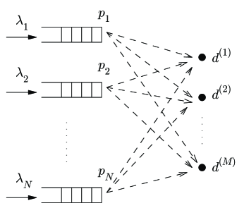
Figure 1: The broadcast scenario we study in this work: $N$ source nodes transmit to $M$ destination nodes.

II-A Queueing stability

Let $Q_{n}(k)$ denote the length of the queue at the $n^{th}$ source node at the beginning of the $k^{th}$ slot in system ${\cal S}$. The evolution of the queue is expressed as follows.

$$Q_{n}(k+1)=\left(Q_{n}(k)-B_{n}(k)\right)^{+}+A_{n}(k),$$ (1)

where $x^{+}=x$ if $x\geq 0$, and 0 otherwise. In the above equation, $A_{n}(k)$ denotes the arrivals to source $n$, where $E[A_{n}(k)]=\lambda_{n},\forall k$ and $B_{n}(k)$ denotes completed services (or departures) from $n$. Thus $B_{n}(k)$ takes value 1 if a packet from source $n$ completes service in slot $k$. We introduce the service rate $\mu_{n}\triangleq\lim_{k\rightarrow\infty}\mbox{Pr}\{B_{n}(k)\}$ as the probability that a packet completes service in the steady-state.

The vector of queue lengths forms an $N$-dimensional, irreducible, aperiodic Markov chain $\mathbf{Q}(k)=(Q_{1}(k),Q_{2}(k),\ldots,Q_{N}(k))$. The system is stable if, for $\mathbf{x}\in\mathbb{N}^{N}$

$$\lim_{\mathbf{x}\rightarrow\infty}\lim_{k\rightarrow\infty}\mbox{Pr}\{\mathbf{Q}(k)<\mathbf{x}\}=1.$$ (2)

For our Markov chain $\mathbf{Q}(k)$, stability is equivalent to positive recurrence of the Markov chain. We define the stability region of the system is the set of all arrival rates $(\lambda_{1},\lambda_{2},\ldots,\lambda_{N})$ for which there exists a set of transmission probabilities $(p_{1},p_{2},\ldots,p_{N})$ such that the system is stable. A primary tool used in our work is Loynes’ result [10], which tells us that if $A_{n}(k)$ and $B_{n}(k)$ are nonnegative, finite, and strictly stationary, then source $n$ is stable if and only if $\lambda_{n}<\mu_{n}$.

II-B Dominant systems

In the original system ${\cal S}$, we cannot easily write down the average service rate $\mu_{n}$ of a source because the service rate varies depending on whether the other sources are empty or backlogged. Instead, we introduce a dominant system ${\cal S}^{[1]}$ which behaves exactly like system ${\cal S}$ except that all $N$ sources continue to transmit “dummy” packets when empty. The dummy packets do not affect the information-carrying ability of the source, but their transmission results in a decoupling of the queues. In the dominant system ${\cal S}^{[1]}$, all sources behave as if they are backlogged, the probability of interference from other sources is known according to the $p_{n}$ values, and we can easily write down the service rates $\mu_{n}^{[1]}$. Let $Q_{n}^{[1]}$ denote the length of the queue at source $n$ in system ${\cal S}^{[1]}$. It can be shown [2] that if $\mu_{n}^{[1]}\leq\mu_{n}$ then $\forall x\in\mathbb{N}$,

$$\mbox{Pr}\{Q_{n}^{[1]}>x\}\geq\mbox{Pr}\{Q_{n}>x\}.$$

In other words, the length of the queue in ${\cal S}^{[1]}$ is never shorter than in ${\cal S}$. So if we find the conditions for stability in ${\cal S}^{[1]}$, then stability in ${\cal S}$ is implied. Thus, stability in the dominant system is a sufficient condition for stability in the original system.

II-C Throughput Region

We define the throughput region of the system as the stability region under the assumption that all sources are always backlogged. As such, we ignore the burstiness of the arrival process. The throughput region of the system ${\cal S}$ is equivalent to the stability region of the dominant system ${\cal S}^{[1]}$. As we noted above, stability in the dominant system ${\cal S}^{[1]}$ implies stability in the original system ${\cal S}$, so the throughput region of the system provides an inner bound to the stability region. It has been conjectured (see [11] and references therein) that the stability region and the throughput region coincide for $N$ sources and a single destination. This conjecture suggests that the zero state $Q_{n}=0$ plays no role in determining the ergodicity of the Markov chain $\mathbf{Q}(k)$. A proof of this conjecture has not been found, and is hindered by the fact that the stability region for $N$ sources has not been found.

III A network of $N$=2 Sources and $M$=2 Destinations

III-A The channel model and service rates

We introduce a channel model similar to the one in [8] to represent the probabilistic reception and MPR that can be attributed to a wireless channel. We define the reception probability when a single source transmits as follows. For $n,m{=}1,2$,

$$q_{n|n}^{(m)}=\mbox{Pr}\{\mbox{packet from source $n$ is received at destination $m$ }|\mbox{ only source $n$ transmits}\}.$$

Additionally, for the $N$=2 scenario, we will include the possibility of capture or MPR with the following reception probability.

$$q_{n|1,2}^{(m)}=\mbox{Pr}\{\mbox{packet from source $n$ is received at destination $m$ }|\mbox{ both sources transmit}\}.$$

If both $s_{1}$ and $s_{2}$ are backlogged, the probability that a packet transmitted from $s_{1}$ is successfully received at both destinations is given by

$$\tau_{1}=\overline{p_{2}}q_{1|1}^{(1)}q_{1|1}^{(2)}+p_{2}q_{1|1,2}^{(1)}q_{1|1,2}^{(2)}$$ (3)

where $\overline{p_{2}}=1-p_{2}$. In general, $\tau_{n},n{=}1,2$ is the probability that a packet from $s_{n}$ is received at both destinations when that source attempts transmission. Similarly, we define $\phi_{n}$ as the probability that a successful reception occurs at $d^{(1)}$ given that $s_{n}$ transmits and $\sigma_{n}$ as the probability that $d^{(2)}$ successfully receives when $s_{n}$ transmits. When both sources are backlogged, $\phi_{1}$ and $\sigma_{1}$ are given by

$$\phi_{1} = \overline{p_{2}}q_{1|1}^{(1)}{+}p_{2}q_{1|1,2}^{(1)}$$ (4)

$$\sigma_{1} = \overline{p_{2}}q_{1|1}^{(2)}{+}p_{2}q_{1|1,2}^{(2)}.$$ (5)

We find the service rates $\mu_{1b}$ and $\mu_{2b}$ for the system in which both sources are backlogged by taking the expected value of $B_{n}$. We first condition $B_{n}$ on the receiver state, where $\mathbf{r_{n}}=(r_{n}^{(1)},r_{n}^{(2)})$ is a vector of binary values indicating whether the packet currently being transmitted by $s_{n}$ has been received at each destination. The possible receiver states are $\mathbf{r_{n}}=\{(0,0),(1,0),(0,1)\}$. We do not allow for the state $(1,1)$ since upon reaching that state, the source will immediately begin serving the next packet. We can write the conditional distribution of $B_{n}$ as given below.

$$\mbox{Pr}\{B_{n}=1|\bf{r_{n}}\}=\begin{cases}p_{n}\tau_{n},&\text{$\mathbf{r_{n}}$=(0,0)}\\ p_{n}\phi_{n},&\text{$\mathbf{r_{n}}$=(0,1)}\\ p_{n}\sigma_{n},&\text{$\mathbf{r_{n}}$=(1,0)}.\end{cases}$$ (6)

To find the expected value of $B_{n}$ we must first find the steady-state probability of each receiver state. The set of receiver states can be modeled by the Markov chain with transition probabilities depicted in Fig. 2. Let $\pi_{0,0}$, $\pi_{0,1}$, and $\pi_{1,0}$ denote the steady-state probabilities of $\bf{r_{n}}$ when both sources are backlogged. Through use of the balance equations for the Markov chain and the equation $\pi_{0,0}+\pi_{0,1}+\pi_{1,0}=1$ we find the steady-state probabilities to be

$$\pi_{0,0} = \frac{\phi_{n}\sigma_{n}}{(\phi_{n}+\sigma_{n})(\phi_{n}+\sigma_{n}-\tau_{n})-\phi_{n}\sigma_{n}}$$

$$\pi_{0,1} = \frac{\sigma_{n}(\sigma_{n}-\tau_{n})}{(\phi_{n}+\sigma_{n})(\phi_{n}+\sigma_{n}-\tau_{n})-\phi_{n}\sigma_{n}}$$

$$\pi_{1,0} = \frac{\phi_{n}(\phi_{n}-\tau_{n})}{(\phi_{n}+\sigma_{n})(\phi_{n}+\sigma_{n}-\tau_{n})-\phi_{n}\sigma_{n}}.$$

Finally, the backlogged service rates $\mu_{nb},n{=}1,2$ can be obtained as $\mu_{nb}=E[B_{n}]=p_{n}\tau_{n}\pi_{0,0}+p_{n}\phi_{n}\pi_{0,1}+p_{n}\sigma_{n}\pi_{1,0}$. After simplification, the backlogged service rates can be expressed as

$$\mu_{nb}=\frac{p_{n}\phi_{n}\sigma_{n}(\phi_{n}+\sigma_{n}-\tau_{n})}{(\phi_{n}+\sigma_{n})(\phi_{n}+\sigma_{n}-\tau_{n})-\phi_{n}\sigma_{n}}.$$ (7)

We let $\mu_{1e}$ denote the service rate of $s_{1}$ when $s_{2}$ is empty and similarly, $\mu_{2e}$ is the service rate of $s_{2}$ when $s_{1}$ is empty. These service rates can be found directly from the backlogged service rates as

$$\mu_{1e}=\Bigl{.}\mu_{1b}\Bigr{|}_{p_{2}=0},\quad\mu_{2e}=\Bigl{.}\mu_{2b}\Bigr{|}_{p_{1}=0}.$$ (8)

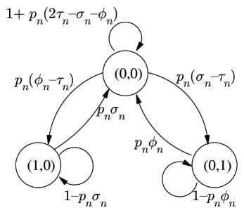
Figure 2: The receiver state Markov chain and transition probabilities for $N=2$ and $M=2$.

III-B Stability and throughput regions

We apply the approach introduced in [3] to find the stability region for $N$=2 and $M$=2. For fixed $(p_{1},p_{2})$ the following theorem provides the condition for stability.

Theorem 1

For a network with $N=2$ sources, $M=2$ destinations, fixed $(p_{1},p_{2})$ and $\mu_{nb}\leq\mu_{ne},n=1,2$, a necessary and sufficient condition for stability is that the arrival rates lie within the union of the following two regions.

$$\lambda_{1}<\frac{\lambda_{2}}{\mu_{2b}}\mu_{1b}+\left(1-\frac{\lambda_{2}}{\mu_{2b}}\right)\mu_{1e},\quad\lambda_{2}<\mu_{2b}.$$ (9)

$$\lambda_{1}<\mu_{1b},\quad\lambda_{2}<\frac{\lambda_{1}}{\mu_{1b}}\mu_{2b}+\left(1-\frac{\lambda_{1}}{\mu_{1b}}\right)\mu_{2e}.$$ (10)

This theorem is a generalization of the result in [3] and the proof follows the one provided in that work. To obtain the stability region over all $(p_{1},p_{2})$ we formulate a constrained optimization problem in which we fix $\lambda_{1}$ and maximize $\lambda_{2}$ over $(p_{1},p_{2})$ subject to Eqns. 9 and 10 [8].

Analyzing the throughput region of the system is equivalent to examining a single dominant system, ${\cal S}^{[1]}$, and the corresponding condition for stability over all $(p_{1},p_{2})$. The stability condition for fixed $(p_{1},p_{2})$ is expressed as

$$\lambda_{1}<\mu_{1b},\quad\lambda_{2}<\mu_{2b}.$$ (11)

We can find points on the boundary of the throughput region by again fixing the value of $\lambda_{1}$ and maximizing $\lambda_{2}$ over $(p_{1},p_{2})$ subject to Eqn. 11. The following theorem states that the throughput region coincides with the stability region; a proof is found in the appendix.

Theorem 2

For a random access broadcast system with $N=2$ source nodes, $M=2$ destination nodes, and service rates as given in (7) and (8), the throughput region is identical to the stability region.

III-C Numerical results

TABLE I: The reception probabilities for results shown in Fig. 3

Channel	$q_{1|1}^{(1)}$	$q_{1|1}^{(2)}$	$q_{1|1,2}^{(1)}$	$q_{1|1,2}^{(2)}$	$q_{2|2}^{(2)}$	$q_{2|2}^{(1)}$	$q_{2|1,2}^{(2)}$	$q_{2|1,2}^{(1)}$
I	0.8	0.6	0.1	0.05	0.7	0.5	0.25	0.05
II	0.8	0.6	0.5	0.4	0.8	0.6	0.5	0.4

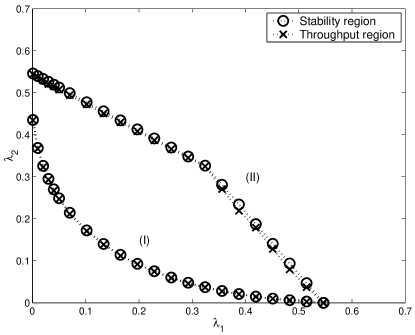
Figure 3: Stability and throughput regions for $N$=2 sources and $M$=2 destinations and two different channel models. The reception probabilities for channels (I) and (II) are shown in Table I.

In Fig. 3 we show the stability and throughput regions computed for two different channels with reception probabilities given in Table I. The figure demonstrates that as the probability of capture or MPR increases, the stability region transforms from a strictly concave region to a convex region bounded by straight lines, which agrees with the results in [8] for unicast transmission. These results also demonstrate that for a network with $N$=2 sources and $M$=2 destinations, the broadcast stability and throughput regions coincide, confirming Theorem 2.

IV A network of $N$ sources and $M$ destinations

IV-A The channel model and service rates

The channel model is now a simplified version of the model presented for the $N$=2, $M$=2 scenario. We assume that whenever two or more sources transmit simultaneously, none of the transmissions are successful. Additionally, we assume that the channel reception probabilities from a source are the same for all destinations, $q_{n|n}^{(1)}=q_{n|n}^{(2)}=\ldots=q_{n|n}^{(M)}=q_{n|n}$, $n=1\ldots N$. We refer to the destinations as being indistinguishable in this channel model.

We define the receiver-state variable $r_{n}$ for each source $n=1,2,\ldots,N$ as the number of destinations that have received the packet that source $n$ is attempting to transmit, $r_{n}\in[0,1,\ldots,M-1]$. We do not allow $r_{n}$ to take value $M$ since as soon as all destinations have received the packet, the source will instantaneously revert back to $r_{n}=0$ and either begin serving the next packet in the queue of source $n$ or become idle if the source is empty. We define the set ${\cal B}$ as the set of all sources that are backlogged at the time source $n$ is attempting to transmit the packet at the front of its queue. Let $\beta_{n}$ denote that probability that source $n$ accesses the channel without interference, i.e.,

$$\beta_{n}=p_{n}\left(\prod_{l\in{\cal B}\setminus n}\overline{p_{l}}\right).$$ (12)

The service process conditioned on $r_{n}$ can be described by

$$\mbox{Pr}\{B_{n}=1|r_{n}=r\}=\beta_{n}{q_{n|n}}^{M-r}.$$ (13)

Figure 4: Receiver state Markov chain for $M$ indistinguishable destinations.

We again develop a Markov chain model for $r_{n}$ as shown in Fig. 4. In this model, transitions “upward” can occur between all pairs of states, however, transitions “downward” can only occur between a state and the $0$ state. Additionally, each state has self-transitions. Let ${\cal P}$ denote the transition matrix for this Markov chain. When source $n$ accesses the channel without collision, which happens with probability $\beta_{n}$, the transition probability matrix will be a matrix ${\cal P^{*}}$ which depends only on the reception probabilities $q_{n|n}$. Otherwise, a self-transition occurs, corresponding to a transition probability matrix equal to the identity matrix ${\cal I}$. Thus, we can describe ${\cal P}$ as the convex combination of two probability matrices,

$${\cal P}=\beta_{n}{\cal P^{*}}+(1-\beta_{n}){\cal I}.$$ (14)

Let $\pi$ be the stationary distribution of ${\cal P^{*}}$, $\mbox{\boldmath$\pi$}=\mbox{\boldmath$\pi$}{\cal P^{*}}$. Clearly $\pi$ will also be the stationary distribution of ${\cal P}$ since $\mbox{\boldmath$\pi$}{\cal P}=\beta_{n}\mbox{\boldmath$\pi$}+(1-\beta_{n})\mbox{\boldmath$\pi$}$. We can solve for $\pi$ as follows. Let $p_{i,j}^{*}$ denote the probability of transition in $r_{n}$ from $i$ to $j$ conditioned on $s_{n}$ accessing the channel without collision. The transition probabilities are given as

$$p_{i,0}^{*}=\begin{cases}(1-q_{n|n})^{M}+q_{n|n}^{M},&i=0\\ q_{n|n}^{M-i},&0<i<M.\end{cases}$$ (15)

$$p_{i,j}^{*}=\begin{cases}(1-q_{n|n})^{M-i},&i=j\\ {M-i\choose j-i}q_{n|n}^{j-i}(1-q_{n|n})^{M-j},&i<j\\ 0,&i>j.\end{cases}$$ (16)

In order to satisfy $\pi_{i}=\sum_{j}\pi_{j}p_{i,j}^{*}$ we have

$$\pi_{i} = \sum_{j=0}^{i-1}\pi_{j}p_{i,j}^{*}+\pi_{i}p_{i,i}^{*}\quad i=1,2,\ldots,M-1$$ (17)

$$= \frac{\sum_{j=0}^{i-1}\pi_{j}p_{i,j}^{*}}{1-p_{i,i}^{*}}$$

$$= \frac{\sum_{k=1}^{i}\pi_{i-k}p_{i-k,i}^{*}}{1-p_{i,i}^{*}}.$$

Together with $\sum_{i=0}^{M-1}\pi_{i}=1$, we can find the steady-state probabilities $\pi$, which is the stationary distribution of ${\cal P}$.

Once the steady-state probabilities of the receiver Markov chain are found, the average service rate is given as follows.

$$\mu_{n}=\beta_{n}\sum_{i=0}^{M-1}\pi_{i}{q_{n|n}}^{M-i}$$ (18)

We further define

$$\alpha_{n}=\sum_{i=0}^{M-1}\pi_{i}{q_{n|n}}^{M-i}.$$ (19)

Thus the service rate can be represented in simplified form as

$$\mu_{n}=\beta_{n}\alpha_{n}.$$ (20)

This equation summarizes the natural relation between our broadcast problem and the unicast collision channel problem [5]. The probability that source $n$ completes transmission of a packet, given by $\mu_{n}$, is equal to $\beta_{n}$, the probability that the source access the channel without collision, times $\alpha_{n}$, which is the probability that all destinations receive the packet conditioned on collision-free access to the channel. In the unicast collision channel problem, we have $q_{n|n}=1$ and $\alpha_{n}=1$. Thus for $\alpha_{n}=1$ we would expect the stability region for our broadcast problem to coincide with the results in [5] for the unicast collision channel. This is indeed the case as shown in the following section.

We define the empty and backlogged service rates as follows. When ${\cal B}$ contains all $N$ sources, the broadcast service rate will take its minimum value $\mu_{nb}$ where

$$\mu_{nb}=p_{n}\left(\prod_{l\neq n}\overline{p_{l}}\right)\alpha_{n}.$$ (21)

The maximum value of $\mu_{n}$ is attained when only source $n$ is backlogged and all other sources are empty. We denote this service rate by $\mu_{ne}$

$$\mu_{ne}=p_{n}\alpha_{n}.$$ (22)

In deriving bounds on the stability region, we will take advantage of the form of $\mu_{n}$ as expressed in Eqn. 20 and the fact that $\mu_{nb}\leq\mu_{n}\leq\mu_{ne}$.

Before continuing, we observe the effect of the number of destinations on the stability and throughput regions as shown in Fig. 5. These results are for $N$=2 sources and $M=2,5,$ and 15 destinations. The results are generated using the approach outlined for $N$=2, $M$=2 with the exception that we use the backlogged and empty service rates for $M$ destinations as given in Eqns. 21 and 22. The results demonstrate that as the number of destinations increases, the broadcast stability and throughput regions diminish in size. Additionally, we observe that the stability and throughput regions coincide. This result is not surprising since the proof of Theorem 2 holds for arbitrary $M$ with the channel model described above.

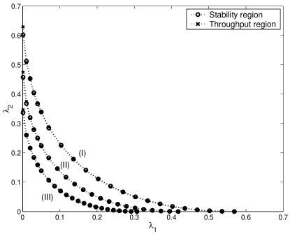
Figure 5: Stability and throughput regions for $N$=2 sources and (I) 2, (II) 5, and (III) 15 destinations.The reception probabilities are: $q_{1|1}=0.7$, $q_{2|2}=0.8$.

IV-B Stability and throughput regions

We follow the methodology outlined in [5] to develop bounds on the broadcast stability region. These results are a generalization of the bounds on the unicast stability region given in [5]. To begin, by the dominant systems argument and Loynes’ result, we can develop loose inner and outer bounds on the stability region. First, if $\lambda_{n}<\mu_{nb}$, then since $\mu_{nb}\leq\mu_{n}$, queue $n$ must be stable. Furthermore, if $\lambda_{n}<\mu_{nb}$ for all $n$, then the entire system is stable. Likewise, if $\lambda_{n}>\mu_{nb}$ for all $n$, then the system is unstable. This follows since $\lambda_{n}>\mu_{nb}$ corresponds to instability of all the queues in dominant system ${\cal S}^{[1]}$, in which case all of the queues grow to infinity and the dominant system ${\cal S}^{[1]}$ becomes indistinguishable from the original system ${\cal S}$ [3]. In order to improve upon these loose bounds, we make use of the stability rank of the queues as introduced in [5]. Let ${\cal S}^{[k]}$ denote a dominant system in which sources $k,k+1,\ldots,N$ transmit dummy packets when empty while sources $1,2,\ldots,k-1$ do not. The proof for the following theorem is the same as in the original [5] with the exception of the constant $\alpha_{n}$.

Theorem 3

Given $\lambda_{N}$ and $\bf{p_{N}}$, we order the indices of the sources so that

$$\frac{\lambda_{1}(1-p_{1})}{\alpha_{1}p_{1}}\leq\ldots\leq\frac{\lambda_{N}(1-p_{N})}{\alpha_{N}p_{N}}.$$ (23)

Then in system ${\cal S}$ and any dominant system ${\cal S}^{[k]}$, if queue $i$ is stable and $j<i$, then queue $j$ is also stable.

We can find conditions for the stability of the system through the procedure outlined in [5]. After ordering the sources according to stability rank, we first check for stability of queue 1 in system ${\cal S}^{[1]}$. If we find that queue 1 is unstable, we can conclude that the entire system is unstable. However, if queue 1 is stable, we proceed by examining queue 2 in system ${\cal S}^{[2]}$. Queue 1 is known to be stable in ${\cal S}^{[2]}$ due to the stability rank. Given stability of queue 1, we will check whether queue 2 is stable in ${\cal S}^{[2]}$. The procedure continues in which the stability of queue $k$ in system ${\cal S}^{[k]}$ is verified assuming that queues $1,2,\ldots,k-1$ are all stable in ${\cal S}^{[k]}$. If we can finally conclude that queue $N$ is stable in system ${\cal S}^{[N]}$, then this implies that the original system is stable.

Assuming that sources $1,2,\ldots,k-1$ are all stable, we will develop bounds on the average service rate $\mu_{k}^{[k]}$ for source $k$ in system ${\cal S}^{[k]}$ in order to help determine whether $s_{k}$ is stable. We can express $\mu_{k}^{[k]}$ as

$$\mu_{k}^{[k]}=\alpha_{k}p_{k}P_{E}^{[k]}\prod_{j=k+1}^{N}(1-p_{j}),$$ (24)

where $P_{E}^{[k]}$ is the probability that none of the sources $1,2,\ldots,k-1$ transmit in the dominant system ${\cal S}^{[k]}$. One way to bound $\mu_{k}^{[k]}$ is by bounding $P_{E}^{[k]}$ when expressed as

$$P_{E}^{[k]}=1-Pr\{\mbox{only one of sources $1,2,\ldots,k-1$ transmits}\}\\ -Pr\{\mbox{more than one of sources $1,2,\ldots,k-1$ transmit}\}.$$ (25)

The bounds on $\mu_{k}^{[k]}$ result in the following two theorems.

Theorem 4

Sufficient condition. Given an $N$ source, $M$ destination random access system with $\lambda_{N}$, $\bf{p_{N}}$ and the sources ordered according to the stability rank as in Eqn. 23, if $\forall k$, $1\leq k\leq N$, $\lambda_{k}<B_{k}$, where $B_{k}$ is defined below, then the system is stable.

$$B_{k} = max(C_{k},D_{k})$$

$$B_{1} = \alpha_{1}p_{1}\prod_{j=2}^{N}(1-p_{j})$$ (26)

$$C_{k} = \frac{\alpha_{k}p_{k}}{1-p_{k}}\left[\prod_{j=k}^{N}(1-p_{j})-\frac{\sum_{i=1}^{k-1}\lambda_{i}}{\min\limits_{1\leq l\leq k-1}\alpha_{l}}-\frac{1}{2}\sum_{j=1}^{k-1}\left(\frac{\lambda_{j}p_{j}}{B_{j}}\prod_{i=k}^{N}(1-p_{i})-\frac{\lambda_{j}}{\alpha_{j}}\right)\right]$$

$$D_{k} = \frac{\alpha_{k}p_{k}}{1-p_{k}}\prod_{j=1}^{N}(1-p_{j})\left(1+\sum_{i=1}^{k-1}\left(1-\frac{\lambda_{i}}{B_{i}}\right)\frac{p_{i}}{1-p_{i}}\right)$$

Theorem 5

Necessary condition. Given an $N$ source, $M$ destination random access system with $\lambda_{N}$, $\bf{p_{N}}$ and the sources ordered according to the stability rank as in Eqn. 23 a necessary condition for stability of the system is that $\forall k$,

$$\lambda_{k}\leq\frac{\alpha_{k}p_{k}}{1-p_{k}}\left(\prod_{j=k}^{N}(1-p_{j})-\frac{\sum_{i=1}^{k-1}\lambda_{i}}{\max\limits_{1\leq l\leq k-1}\alpha_{l}}\right).$$ (28)

The proofs for Theorems 4 and 5 are described in the Appendix. We make use of these two theorems to develop bounds on the stability region by fixing the values of $\lambda_{1},\lambda_{2},\ldots,\lambda_{N-1}$ and numerically optimizing $\lambda_{N}$ over all $\mathbf{p_{N}}\in[0,1]^{N}$ subject to the inequalities given in the Theorems.

The throughput region of the network of arbitrary size can be determined exactly using the backlogged service rates in Eqn. 21. Again, we fix $\lambda_{1},\lambda_{2},\ldots,\lambda_{N-1}$ and maximize $\lambda_{N}$ over all $\bf{p_{N}}$ subject to $\lambda_{N}<\mu_{Nb}$.

IV-C Numerical results

TABLE II: Optimization results of stability bounds and throughput for a network of $N$=4 sources and $M$=8 and 10 destinations. The values of $\lambda_{1},\lambda_{2},$ and $\lambda_{3}$ were fixed and $\lambda_{4}$ has been optimized over all $\mathbf{p}$.

$M$	$q_{1|1}$	$q_{2|2}$	$q_{3|3}$	$q_{4|4}$	$\lambda_{1}$	$\lambda_{2}$	$\lambda_{3}$	Stability-upper	Stability-lower	Throughput
8	0.9	0.8	0.7	0.9	0.01	0.01	0.01	0.3648	0.3213	0.3213
					0.07	0.02	0.01	0.2125	0.1672	0.1672
					0.05	0.05	0.05	0.1363	0.0566	0.0566
					0.07	0.05	0.05	0.1090	0.0376	0.0376
8	0.8	0.8	0.8	0.8	0.01	0.01	0.01	0.2527	0.2433	0.2434
					0.07	0.02	0.01	0.1294	0.1090	0.1090
					0.05	0.05	0.05	0.0784	0.0428	0.0428
					0.07	0.05	0.05	0.0587	0.0254	0.0254
10	0.8	0.8	0.8	0.8	0.01	0.01	0.01	0.2329	0.2236	0.2236
					0.07	0.02	0.01	0.1153	0.0951	0.0951
					0.05	0.05	0.05	0.0651	0.0318	0.0321
					0.065	0.05	0.05	0.0503	0.0196	0.0196

TABLE III: Optimization results of stability bounds and throughput for a network of $N$=5 and 10 sources and $M$=10 destinations. The reception probabilities are $q_{n|n}=0.8$ for $n=1,\ldots,N$. The values of $\lambda_{1},\ldots,\lambda_{N-1}$ were fixed and $\lambda_{N}$ has been optimized over all $\mathbf{p}$.

$N$	$\lambda_{1},\ldots,\lambda_{N-1}$	Stability-upper	Stability-lower	Throughput
5	$[0.010,0.010,0.010,0.010]$	0.2078	0.1939	0.1939
	$[0.070,0.020,0.010,0.010]$	0.1051	0.0789	0.0789
	$[0.035,0.035,0.035,0.035]$	0.0751	0.0362	0.0362
	$[0.050,0.035,0.035,0.035]$	0.0602	0.0223	0.0223
10	$[0.010,0.010,\ldots 0.010]$	0.1266	0.0912	0.0912
	$[0.070,0.010,\ldots 0.010]$	0.0679	0.0252	0.0252
	$[0.017,0.017,\ldots 0.017]$	0.0621	0.0137	0.0137
	$[0.020,0.017,\ldots 0.017]$	0.0591	0.0108	0.0108

A collection of results on stability and throughput for various values of $N$ and $M$ are shown in Tables II and III. The values in Table II demonstrate the effect of the channel reception probabilities and the number of destinations on the stability and throughput regions. The trends in these results are the same as those observed for a network of $N$=2 sources. In Table III we observe that as the number of sources $N$ increases, the stability and throughput regions diminish in size. Furthermore, in all cases, the throughput values fall within the upper and lower bounds on the stability values. As such, these results support the conjecture that the stability and throughput regions coincide. Of special note, the lower bound for stability and the throughput value appear to be equal in many cases. This is not entirely true. In the results shown here, the throughput value is in fact slightly larger than the lower bound on the stability value, but the difference is at most $10^{-6}$.

V Conclusions

In this work we have investigated the information-carrying ability of source nodes which compete for access to a shared channel in order to broadcast messages to a common set of destination nodes. The scenario we consider is relevant to broadcast applications and network discovery and control. We formulated the problem as a network of queues which interact through the shared channel and investigated the stability and throughput regions of the source nodes. Our results strengthen an unproven conjecture that the stability and throughput regions of finite-user random access coincide. We also demonstrate that the throughput and stable throughput regions diminish as the number of source or destination nodes grows. Our intention in this work is to present results relating to the scaling laws for wireless networks, which often show a degradation in throughput as the number of nodes increases. Our results show a similar trend from a multicast stability point of view.

VI Appendix

VI-A Proof of Theorem 2

We show that the boundaries of the stability and throughput regions, given by the results of two constrained optimization problems, are identical. We replace $\lambda_{1}$ by $x$ and $\lambda_{2}$ by $y$. Furthermore, we express the backlogged service rates $\mu_{nb}$ in Eqn. 7 as follows.

$$\mu_{1b}=p_{1}f_{1}(p_{2}),\quad\mu_{2b}=p_{2}f_{2}(p_{1}).$$ (29)

The empty service rates can then be expressed as $\mu_{1e}=p_{1}f_{1}(0)$ and $\mu_{2e}=p_{2}f_{2}(0)$. In these expressions, $f_{1}(p_{2})$ is functionally independent of $p_{1}$ and decreasing in $p_{2}$, corresponding to $\mu_{1b}\leq\mu_{1e}\iff f_{1}(p_{2})\leq f_{1}(0)$. Similarly, $f_{2}(p_{1})$ is independent of $p_{2}$ and decreasing in $p_{1}$. With this notation in place, the boundary of the region given in Theorem 1 for fixed $(p_{1},p_{2})$ can be written as follows.

$$x=p_{1}f_{1}(0)-\frac{yp_{1}\left(f_{1}(0)-f_{1}(p_{2})\right)}{p_{2}f_{2}(p_{1})},\quad 0\leq y\leq p_{2}f_{2}(p_{1})$$ (30)

$$y=p_{2}f_{2}(0)-\frac{xp_{2}\left(f_{2}(0)-f_{2}(p_{1})\right)}{p_{1}f_{1}(p_{2})},\quad 0\leq x\leq p_{1}f_{1}(p_{2})$$ (31)

To find the stability region, we should maximize the expressions in (30) and (31) over $(p_{1},p_{2})$ and take the intersection of the regions bounded by the resulting curves. We note that this is not a standard optimization problem because the objective function is piece-wise and non-differentiable at a point in its domain. An example of an analytical solution to this optimization problem is given in [8] for the single destination case.

The boundary of the throughput region for fixed $(p_{1},p_{2})$ as given in Eqn. 11 can be written as follows.

$$x=p_{1}f_{1}(p_{2}),\quad 0\leq y\leq p_{2}f_{2}(p_{1})$$ (32)

$$y=p_{2}f_{2}(p_{1}),\quad 0\leq x\leq p_{1}f_{1}(p_{2})$$ (33)

The throughput region is found by maximizing the expressions in (32) and (33) and taking the intersection of the resulting regions. Consider Eqn. (33) in which we wish to maximize $y$ over $(p_{1},p_{2})$. Note that the constraint $x\leq p_{1}f_{1}(p_{2})$ is a lower bound on $p_{1}$ over which we perform the maximization. Since $f_{2}(p_{1})$ is decreasing in $p_{1}$, the lower bound $p_{1}\geq x/f_{1}(p_{2})$ provides an upper bound on $y$, and this upper bound can be achieved when maximizing (33) over $(p_{1},p_{2})$. Then maximization of $y$ in (33) is equivalent to maximizing $y$ as follows.

$$y=\biggl{.}p_{2}f_{2}(p_{1})\biggr{|}_{p_{1}=\tfrac{x}{f_{1}(p_{2})}},\quad 0\leq x\leq p_{1}f_{1}(p_{2})$$ (34)

To see that this is identical to (31), we write $f_{2}(p_{1})$ as follows.

$$f_{2}(p_{1}) = f_{2}(0)-\left(f_{2}(0)-f_{2}(p_{1})\right)$$ (35)

$$= f_{2}(0)-\frac{p_{1}\left(f_{2}(0)-f_{2}(p_{1})\right)}{p_{1}}$$ (36)

Then

$$\biggl{.}p_{2}f_{2}(p_{1})\biggr{|}_{p_{1}=\tfrac{x}{f_{1}(p_{2})}}=p_{2}f_{2}(0)-\frac{xp_{2}\left(f_{2}(0)-f_{2}(p_{1})\right)}{p_{1}f_{1}(p_{2})}$$ (37)

and the maximum $y$ in (33) is identical to the maximum $y$ in (31). Similarly, the maximum of $x$ in (32) is identical to the maximum of $x$ in (30).

VI-B Proof of Theorem 4

Our proof follows the one given in [5]. A sufficient condition for stability corresponds to bounding $\mu_{k}^{[k]}$ from below. We obtain two separate lower bounds, $C_{k}$ and $D_{k}$, and take their maximum to obtain the result. The bound $C_{k}$ is derived through Eqns. 24 and 25. Since sources $1,2,\ldots,k-1$ are stable, the following holds.

$$Pr\{\mbox{success by one of the sources $1,2,\ldots,k-1$}\}=\sum_{i=1}^{k-1}\lambda_{i}\\ \geq\left(\min_{1\leq l\leq k}\alpha_{l}\right)Pr\{\mbox{only one of the sources $1,2,\ldots,k-1$ transmits}\}\prod_{j=k}^{N}(1-p_{j})$$ (38)

This indicates that

$$Pr\{\mbox{only one of the sources $1,2,\ldots,k-1$ transmits}\}\leq\frac{\sum_{i=1}^{k-1}\lambda_{i}}{\left(\min\limits_{1\leq l\leq k}\alpha_{l}\right)\prod_{j=k}^{N}(1-p_{j})}.$$ (39)

For the next term in $P_{E}^{[k]}$ we have

$$Pr\{\mbox{a packet from $j$ collides with others from $1,2,\ldots,k-1$}\}\\ =Pr\{\mbox{$j$ transmits}\}-Pr\{\mbox{$j$ transmits \& no others from $1,2,\ldots,k-1$ transmit}\}\\ =p_{j}Pr\{\mbox{$j$ backlogged}\}-\frac{Pr\{\mbox{$j$ transmits \& no others transmit}\}}{\prod_{i=k}^{N}(1-p_{i})}\\ =p_{j}\frac{\lambda_{j}}{\mu_{j}^{[k]}}-\frac{\lambda_{j}}{\alpha_{j}\prod_{i=k}^{N}(1-p_{i})}.$$ (40)

We also make use of the result shown in [3] that for $j<k$, $\mu_{j}^{[j]}\leq\mu_{j}^{[k]}$. Thus, the second term in $P_{E}^{[k]}$ is upper bounded as follows.

$$Pr\{\mbox{more than one of the sources $1,2,\ldots,k-1$ transmits}\}\leq\frac{1}{2}\sum_{j=1}^{k-1}\left(p_{j}\frac{\lambda_{j}}{\mu_{j}^{[j]}}-\frac{\lambda_{j}}{\alpha_{j}\prod_{i=k}^{N}(1-p_{i})}\right)$$ (41)

By combining Eqns. 25, 39, and 41 we obtain the lower bound

$$P_{E}^{[k]}\geq 1-\frac{\sum_{i=1}^{k-1}\lambda_{i}}{\left(\min\limits_{1\leq l\leq k}\alpha_{l}\right)\prod_{j=k}^{N}(1-p_{j})}-\frac{1}{2}\sum_{j=1}^{k-1}\left(p_{j}\frac{\lambda_{j}}{\mu_{j}^{[j]}}-\frac{\lambda_{j}}{\alpha_{j}\prod_{i=k}^{N}(1-p_{i})}\right).$$ (42)

Together with Eqn. 24, this provides $C_{k}$, our first lower bound on $\mu_{k}^{[k]}$.

The other lower bound on $\mu_{k}^{[k]}$ is derived using an approach from [3]. We have adapted it for the broadcast problem below and refer to it as $D_{k}$.

$$\mu_{k}^{[k]}\geq\frac{\alpha_{k}p_{k}}{1-p_{k}}Pr\{\mbox{no other source transmits}\}\\ +\frac{\alpha_{k}p_{k}}{1-p_{k}}Pr\{\mbox{one of the first $1,2,\ldots,k-1$ sources transmits but is empty}\}\\ =\frac{\alpha_{k}p_{k}}{1-p_{k}}\prod_{j=1}^{N}(1-p_{j})\left(1+\sum_{i=1}^{k-1}\left(1-\frac{\lambda_{i}}{\mu_{i}^{[i]}}\right)\frac{p_{i}}{1-p_{i}}\right)=D_{k}.$$ (43)

Note that we can express the exact value of $\mu_{1}^{[1]}$ as $\mu_{1}^{[1]}=\alpha_{1}p_{1}\prod_{j=2}^{N}(1-p_{j})$. By beginning with $B_{1}=\mu_{1}^{[1]}$ we can iterate through $k$ values $2,\ldots,N$ to obtain the result.

The proof of Theorem 5 develops upper bounds on $\mu_{k}^{[k]}$ and thus on $P_{E}^{[k]}$. The technique is similar to the one outlined above in finding $C_{k}$.

References

- [1] N. Abramson, “The throughput of packet broadcasting channels,” IEEE Trans. Commun., vol. COM-25, pp. 117–128, January 1977.
- [2] B. Tsybakov and V. Mikhailov, “Ergodicity of a slotted aloha system,” Probl. Inform. Tran, vol. 15, pp. 301–312, 1979.
- [3] R. Rao and A. Ephremides, “On the stability of interacting queues in a multiple-access system,” IEEE Trans. Inform. Theory, vol. 34, pp. 918–930, September 1988.
- [4] W. Szpankowski, “Stability conditions for some distributed systems: Buffered random access systems,” Advances in Applied Probability, vol. 26, pp. 498–515, June 1994.
- [5] W. Luo and A. Ephremides, “Stability of n interacting queues in random-access systems,” IEEE Trans. Inform. Theory, vol. 45, pp. 1579–1587, July 1999.
- [6] V. Anantharam, “Stability region of the finite-user slotted aloha protocol,” IEEE Trans. Inform. Theory, vol. 37, pp. 535–540, May 1991.
- [7] S. Ghez, S. Verdu, and S. Schwartz, “Stability properties of slotted aloha with multipacket reception capability,” IEEE Trans. Auto. Control, vol. 33, July 1988.
- [8] V. Naware, G. Mergen, and L. Tong, “Stability and delay of finite user slotted aloha with multipacket reception,” IEEE Trans. Inform. Theory, vol. 51, pp. 2636–2656, July 2005.
- [9] J. I. Capetanakis, “Tree algorithms for packet broadcast channels,” IEEE Trans. Inform. Theory, vol. 25, pp. 505–515, September 1979.
- [10] R. Loynes, “The stability of a queue with non-independent interarrival and service times,” Proc. Cambridge Phil. Soc., vol. 58, 1962.
- [11] J. Luo and A. Ephremides, “On the throughput, capacity and stability regions of random multiple access,” IEEE Trans. Inform. Theory, vol. 52, pp. 2593–2607, June 2006.