Why should anyone care about computing with anyons?

Abstract

Topological Quantum Computation, Topological models.

In this article we present a pedagogical introduction of the main ideas and recent advances in the area of topological quantum computation. We give an overview of the concept of anyons and their exotic statistics, present various models that exhibit topological behavior, and we establish their relation to quantum computation. Possible directions for the physical realization of topological systems and the detection of anyonic behavior are elaborated.

1 Introduction

The objectives of current research in quantum computation are mainly twofold. Firstly, to perform neat quantum evolutions, robust against decoherence and control errors. Secondly, to find new quantum algorithms that outperform their classical counterparts. Topological quantum systems have been proven to be a fertile environment for addressing both of these questions. In particular, topological quantum computation is concerned with two dimensional many body systems that support excitations with exotic statistics called anyons. Encoding and manipulating information with anyons is an intrinsically error free procedure. If physically realized it could allow reliable quantum computation without the need of the huge error correction overhead. Moreover, it has provided the setup for constructing a new quantum algorithm inspired from the evolution of topological excitations. This algorithm can approximated the Jones polynomials, topological invariants that can distinguish between inequivalent knots. The exact evaluation of the Jones polynomials is an exponentially hard classical problem with much interest in various fields such as in biology, through the protein folding problem, and in statistical physics.

Topological quantum systems are more familiar from the Quantum Hall Effect where a two dimensional layer of electrons is subject to a strong vertical magnetic field. The low energy spectrum of these systems is governed by a trivial Hamiltonian, $H=0$. Nevertheless, they have an interesting behavior due to the non-trivial statistics of their excitations. It has been proven that this behavior is dictated by the presence of anyons. Unlike bosons or fermions, anyons have a non-trivial evolution when one circulates another. Lately, lattice counterparts to these continuous systems have been proposed that can also support anyonic excitations. These spin or electron systems offer an alternative way of generating and manipulating anyons that can also support topological quantum computation.

Here we will give a pedagogical presentation of various inspiring ideas related to topological quantum computation that manifests the close relation between physics, mathematics and information theory. We will present several topological systems, explain their relevance to error free quantum computation and give possible physical realizations with cold atomic systems. The interested reader may refer to the bibliography for the in depth analysis of the subjects presented here.

2 Anyons: what are they?

It is commonly accepted that point-like particles, elementary or not, come in two species: bosons or fermions. The particle label is determined by the behavior of their wave function: if two identical non-interacting particles are exchanged we expect that their wavefunction will acquire either a plus sign (bosons) or a minus sign (fermions). These are the only observed statistical behaviors for particles that exist in our three dimensional world. Indeed, circulating a particle around an identical one spans a path that in three dimensions can be continuously deformed to a trivial path as seen in Figure 1.

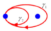
Figure 1: A particle spans a loop around another one. In three dimensions it is possible to continuously deform the path $\gamma_{1}$ to the path $\gamma_{2}$ which is equivalent to a trivial path.

As a consequence the wave function, $\left|\Psi(\gamma_{1})\right\rangle$, of the system after the circulation has to be exactly the same as the original one $\left|\Psi(0)\right\rangle$, i.e.

$$\left|\Psi(\gamma_{1})\right\rangle=\left|\Psi(\gamma_{2})\right\rangle=\left|\Psi(0)\right\rangle$$ (1)

It is easily seen that a full circulation is equivalent to two successive particle exchanges. Thus, a single exchange can result to a phase factor $e^{i\varphi}$ that has to square to unity in order to be consistent with (1), giving, finally, $\varphi=0,\pi$. These two cases correspond to bosonic and fermionic statistics respectively.

When we restrict to two spatial dimensions there are more possibilities in the statistical behavior of the particles. If the particle circulation $\gamma_{1}$ of Figure 1 is performed on a plane, then it is not possible to continuously deform it to the path $\gamma_{2}$. Still the evolution that corresponds to $\gamma_{2}$ is equivalent to the trivial evolution as seen in Figure 2. As we are not able to deform the evolution of path $\gamma_{1}$ to the trivial one, it is possible to assign an arbitrary phase factor or even a whole unitary to this evolution. Thus, particles in two dimensions can have richer statistical behavior different from bosons or fermions.

To visualize the behavior of anyons one can think of them as being composite particles consisting of a flux $\Phi$ and a ring of charge $q$ as depicted in Figure 2.

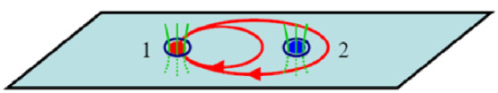
Figure 2: In two dimensions the two paths $\gamma_{1}$ and $\gamma_{2}$ are topologically distinct. This gives the possibility of having non-trivial phase factors appearing when one particle circulates the other. This can be visualized by having the particles carrying charge as well as magnetic flux giving rise to the Aharonov-Bohm effect.

If the particle $1$ circulates particle $2$ then its charge $q$ goes around the flux $\Phi$ thus acquiring a phase factor $U=e^{iq\Phi}$ due to the Aharonov-Bohm effect. The statistical angle of these anyons is then $\varphi=q\Phi/2$. Non-abelian charges and fluxes can generate unitary matrices instead of phase factors. In this case a circulation of one anyon around another can lead to a final state in superposition. The anyons that have such statistics are called non-abelian, while anyons that obtain a simple phase factor are called abelian. Note that the generation of the evolution is not a result of a direct interaction but rather a topological consequence as in the Aharonov-Bohm effect. In reality the presence of charge and flux come from an effective gauge theory that describes the low energy behavior of the model.

As the statistical properties dominate the behavior of the anyonic states, it is convenient to employ the world lines of the particles to keep track of their positions. In this way exchanges of the anyons can be easily describe just by braiding their world lines. Moreover, we can depict the pair creation of anyon anti-anyon from the vacuum as well as their annihilation (see Figure 3).

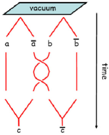
Figure 3: The world lines of the anyons where the third dimension depicts time running downwards. From the vacuum two pairs of anyon and anti-anyon are generated depicted by $(a,\bar{a})$ and $(b,\bar{b})$. Then anyons $\bar{a}$ and $b$ are braided by circulating one around the other. Finally, the anyons are pairwise fused, but they do not necessarily return to the vacuum as the braiding process may have changed their internal state.

Out of the vacuum an anyon and an anti-anion are generated with a local physical process. We assume that we can trap and move the anyons around the plane leading to world lines in $2+1$ dimensions. In the particular depicted example two pairs of anyons are created $(a,\bar{a})$ and $(b,\bar{b})$. Then anyons $\bar{a}$ and $b$ are braided by circulating one around the other and then the corresponding pairs are fused. The fusion may not result to the vacuum as the braiding process could change the internal state of one of the anyons. The outcomes of the fusions are the anyons $c$ and $\bar{c}$. They can be further fused giving the vacuum that we had started with in agreement with the conservation of the relevant quantum numbers.

As we have seen the generation of the anyons with pair creation results in well defined pair of anyon anti-anyon. When two anyons are fused, it is possible to have various outcomes depending on their internal state. In Figure 3, one can see that the fusions result in the anyons $c$ and $\bar{c}$. In general, depending in the particular internal state of the anyons, one can have different unique outcomes from the fusion. This is denoted in the following way

$$a\times b=N^{c}_{ab}c+N^{d}_{ab}d+...$$ (2)

where anyons $a$ and $b$ are fused to produce either anyon $c$ or $d$ or any other possible outcome. The order of the outcomes in the sum is not important. The integers $N_{jk}^{l}$ denote the multiplicity that the particles $l$ are generated out of the fusion of the particles $j$ and $k$. This is similar to the tensor product of spins that results in a new spin basis, e.g. ${1\over 2}\otimes{1\over 2}=0\oplus 1$. In particular abelian anyons have only a single fusion product $a\times b=c$, while for non-abelian anyons the outcome of the fusion is not unique. In particular, one can assign a unitary matrix $F$ that transforms between the different ways that three anyons can fuse to give a fourth one.

Apart from the fusion rules we are also interested in the statistics of the anyons. The latter is characterized by the unitary $R$ that describes the evolution of the anyonic states when the anyons are anticlockwise interchanged (see Figure 4(a)).

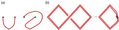
Figure 4: (a) Two anyons are exchanged with paths attached to them from a common reference point. The exchange is described by a unitary matrix $R$ acting on the state of the anyons. (b) The equivalence between spin and statistics. Two anyons, each one from two anyon anti-anyon pairs, are exchanged and recombined fusing to the vacuum. This process is equivalent to rotating one anyon by $2\pi$ from a pair and recombining them causing an evolution due to the spin of the anyon. The anyons are depicted here as ribbons to keep track of their spin rotation.

The interpretation of the anyons with world lines, and in particular with “world ribbons” makes apparent the connection between statistics and spin. Indeed, in Figure 4 we see the schematical equivalence between the process of exchanging two abelian anyons and the rotation of an anyon by $2\pi$. The first is evolved by the statistical unitary $R$ (a phase factor for abelian anyons) and the second is expected to obtain a phase factor $e^{i2\pi J}$, where $J$ is the spin of the anyon. A direct application leads to the connection between the integer spins for bosons and half integer spins for fermions. This is in agreement with the interpretation of anyons as a composite object of charge and flux. In this case the rotation of an anyon by $2\pi$ will rotate the charge around the flux leading to the same phase factor dictated by their statistics due to the Aharonov-Bohm effect.

Finally, one can show that consistency equations can be considered that give a relation between the statistical processes and the fusion relations. Two such basic processes, the braiding of two anyons and the reordering of the fusion of three anyons are given by the unitaries $R$ and $F$, respectively. These consistency equations are called pentagon and hexagon equations ( Turaev 1994).

3 Surface codes

The marriage of topology and quantum information began with a proposal (Kitaev 1997) for encoding quantum information in the collective state of interacting spins on a surface. Such codes are known as surface codes and have several desirable characteristics. First the information is encoded in a subspace of the state-space of the spins, whose dimension is a property of the topology of the surface alone. This is a global property robust to local perturbations. Second, this codespace corresponds to the degenerate ground subspace of a Hamiltonian that is quasi-local. Here quasi-local means that the interactions take place only among a few neighboring particles (typically $3-6$). This is in stark contrast with most other quantum error correction codes which do not correspond to the ground state of any quasi-local Hamiltonian. Also, the ground states possess a symmetry. They are invariant under the action of a product of connected local spin operators which form a closed loop, while the action of an open string of operators creates excitations at its endpoints. The ground states are isolated from low lying excited states by an energy gap which remains finite in the thermodynamic limit. Provided the temperature of the environment is much less than this gap, the probability of errors (excitations) is small. Third, any local errors that do arise are characterized as anyonic quasiparticle pairs, whose mass is proportional to the energy gap. These anyons are positioned at the ends of the open string operations acting on the vacuum (ground states). All that is required to correct the errors is to annihilate the anyons by connecting the string ends along a closed loop that is homologically trivial, i.e. it can be contracted to a point. Logical operations on the codespace correspond to loops of operations that are topologically non-trivial, i.e. they cannot be shrunk to a point loop.

Generically, surface codes appear as ground states of Hamiltonians involving spins residing on a surface. They are best understood in terms of a coupling graph, where each physical spin is represented by an edge on the graph. The Hamiltonian is a sum of two types of interactions: a vertex term $H_{v}$ involving interactions between all edges that meet at a vertex, and a face term $H_{f}$ describing interactions between all edges that surround a face. An important geometric constraint is that any vertex interaction shares at most two edges with any face interaction. When the operators $H_{v}$ and $H_{f}$ commute, then it can be shown that the model can support topologically ordered ground states. For example, consider a square lattice of spin-$1/2$ particles, or qubits, with the Hamiltonian

$$H=-U\sum_{v}H_{v}-J\sum_{f}H_{f}$$ (3)

for $U,J>0$. The interactions look like a product of operations on a cross $H_{v}=\prod_{e\in+}Z_{e}$ or a square $H_{f}=\prod_{e\in\square}X_{e}$, where $Z$ and $X$ are the corresponding Pauli operators. Each vertex (face) operator involves a product of two or zero $Z(X)$ operators on any face (vertex). Since the Pauli operators anticommute, even products of them commute, hence $[H_{v},H_{f}]=0$. For this reason the states can be labelled according to the eigenvalues of the set of operators $\{H_{v},H_{f}\}$. The ground states of $H$ are $+1$ eigenstates of this set hence the vertex and face operators are stabilizers. However, not all the stabilizers are independent. For instance, on a torus, $\prod_{v}H_{v}={\bf 1}_{2^{n}}$ and $\prod_{f}H_{f}={\bf 1}_{2^{n}}$, hence there are only $n-2$ independent stabilizers. Eigenspaces of $H$ are labeled according to the $\pm 1$ eigenvalues of the independent stabilizer operators and the ground state degeneracy is therefore $2^{n}/2^{n-2}=4$. For a surface of genus $g$ the degeneracy is $2^{2g}$ with ground states that are indistinguishable by local observables. This spectral property is called topological degeneracy. An example of a surface code on a planar surface with non-trivial topology is shown in Figure 5.

The model above describes an effective $\mathbb{Z}_{2}$ gauge theory where the generators of local gauge transformations are $\{H_{v},H_{f}\}$. Excitations above the vacuum ground state behave like particles which have anyonic statistics. Indeed, the local operation $Z_{e}$ creates a $\mathbb{Z}_{2}$ valued charge and anti-charge with total mass $2U$ on the boundaries of edge $e$, and $X_{e}$ creates a $\mathbb{Z}_{2}$ valued flux anti-flux pair with total mass $2J$ on faces sharing the common boundary edge $e$. The operation $Y_{e}$ creates a dyonic combination of charge anti-charge and flux anti-flux pairs. The relative statistical obtained by winding a charge/flux dyon $(r,s)$ around another dyon $(r^{\prime},s^{\prime})$ is $\phi^{(r,s)}_{(r^{\prime},s^{\prime})}=\pi(rs^{\prime}+sr^{\prime})$ as illustrated in Figure 5. One can generalize the Hamiltonian (Eq. 3) to higher spin systems with $d$ levels, or qudits, that gives rise to an effective $\mathbb{Z}_{d}$ gauge theory with topological degeneracy $d^{2g}$ (Bullock and Brennen 2007). Here the quasiparticles are $d$ valued integers and the relative statistical phase is $\phi^{(r,s)}_{(r^{\prime},s^{\prime})}=\frac{2\pi}{d}(rs^{\prime}+sr^{\prime})$. As before, this phase can be derived from the commutator for the generalized Pauli group on qudits: $Z^{r}X^{s}=e^{i2\pi rs/d}X^{s}Z^{r}$

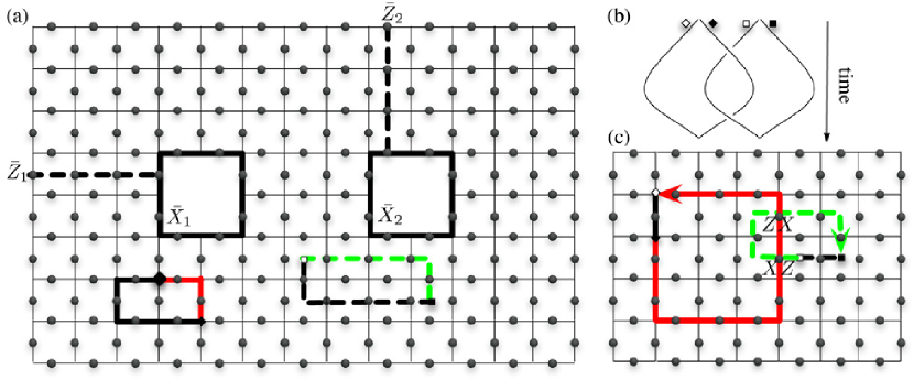
Figure 5: Surface codes and anyonic excitations. (a) A twice punctured plane encoding $2$ qubits. Physical qubits (grey dots) reside on the edges and a black solid (dashed) string intersecting a qubit corresponds to a physical $X(Z)$ operation on that qubit. The logical operations $\bar{X}_{1,2}$ correspond to non-trivial loops around the punctures while the logical $\bar{Z}_{1,2}$ connect boundaries. This code protects against $3$ bit flip errors and $2$ phase errors but a more resilient code results by increasing the lattice size. Correctible errors are shown in the lower half of the surface. String boundaries, denoted by $\square$ or $\diamond$ indicate where a vertex or face stabilizer condition is violated. These errors can be corrected by connecting the string ends along a contractible loop (red and green strings). (b) The action of braiding a charge $(\diamond)$ around a flux $(\square)$. For a $\mathbb{Z}_{2}$ gauge theory, particles and anti-particles are equivalent. (c) Configuration path for the braiding beginning in the vacuum, i.e. a ground state. The action on the state is obtained by interchanging the order of operations on one intersecting edge. Since $ZX=-XZ$, and contractible loops act trivially on the vacuum (ground states), the resultant action on the wavefunction after braiding is $U=\exp[i\phi^{(1,0)}_{(0,1)}]=-1$.

4 Fibonacci Anyons for quantum computation

In this section we will present probably the most celebrated non-abelian anyonic model not only due to its simplicity and richness in structure, but also due to its connection to the Fibonacci series. In this model there are two different types of anyons, $0$ and $1$, that have the following fusion rules

$$0\times 0=0,\,\,\,0\times 1=1,\,\,\,1\times 1=0+1$$

It is interesting to study all the possible outcomes when we fuse many anyons of type $1$.

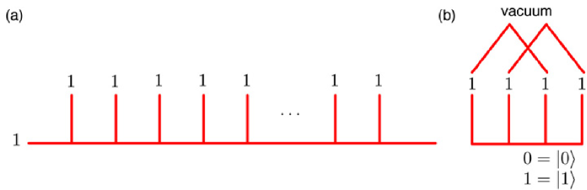
Figure 6: Depiction of the fusion process for anyons. (a) A series of $1$ anyons are fused together going from left to right. The first two $1$ anyons are fused and then their outcome is fused with the next $1$ anyon and so on. (b) Four Fibonacci anyons in state $1$ created from the vacuum can be used to encode a single logical qubit. When restricted to the space of trivial total charge, there are two distinguishable ways the particles can be fused together, indicated by $0$ and $1$. This state space is sufficient to encode a logical qubit.

For this we fuse the first two anyons and then their outcome is fused with the third $1$ anyon and the single outcome is fused with the next one and so on. As the $1$ anyons have two possible fusion outcome states it is natural to ask what are the number of ways, $d_{1}(n)$, one can fuse $n+1$ anyons of type $1$ to yield a $1$. At the first fusing step the possible outcomes are $0$ or $1$, giving $d_{1}(2)=1$. When we fuse the outcome with the next anyon then $0\times 1=1$ and $1\times 1=0+1$, resulting to two possible $1$’s coming from two different processes and a $0$, i.e. $d_{1}(3)=2$. Taking the possible outcome and fusing it with the next anyon gives a space of $1$’s which is three dimensional $d_{1}(4)=3$. The series of the space dimension $d_{1}(n)$ when $n+1$ anyons of type $1$ are fused is actually the Fibonacci series. This dimension, $d_{1}(n)$, is also called the dimension of the fusion space and is given approximately by the following formula

$$d_{1}(n)\propto\phi^{n}$$

where $\phi\equiv(1+\sqrt{5})/2$ is the Golden Mean. The latter has been used extensively by artists, such as Leonardo Da Vinci, in geometrical representations of nature (plants, animals or humans) to describe the ratios that are aesthetically appealing. The above calculation is helpful to illustrate the counting of Hilbert space dimension, however, there is a more systematic way to compute the state space dimension using the concept of quantum dimension. The quantum dimension $d_{\alpha}$ quantifies the rate of growth of Hilbert space dimension $d_{\alpha}(n)$ when one additional particle of type $\alpha$ is added. From another perspective, the ratio $1/d_{\alpha}^{2}$ is the probability that a particle of type $\alpha$ and its antiparticle of type $\bar{\alpha}$ will annihilate. The dimension satisfies the following product rule: $d_{a}d_{b}=\sum_{c}N^{c}_{ab}d_{c}$. Thus, for the Fibonacci model the quantum dimensions for the two particles types can easily be solved for from the fusion rules in Eq. 4: $d_{0}^{2}=d_{0}=1$ and $d_{1}^{2}=1+d_{1}\rightarrow d_{1}=\phi$.

This anyonic system is a good example for realization of quantum computation. We are interested in encoding information in the fusion space of anyons and then processing it appropriately. This is an algorithmically equivalent, but physically completely different way of encoding and processing information compared to the circuit model. In the latter, qubits are positioned in space and the logical gates are applied as a series of unitary evolutions.

There have been several proposals of quantum computation that are conceptually different, but equivalent to the circuit model. By equivalent we mean that any model can simulate another with at most a polynomial overhead in the number of operations that determine the complexity of implementation. One way quantum computation (Raussendorf and Briegel 2001) starts from a large entangled state. Information is then processed by single qubit measurements in contrast to the popular belief that quantum computation must be reversible. Adiabatic quantum computation is another way of processing information (Farhi et al. 2001). There, the answer to the problem is encoded into the unique ground state of a Hamiltonian. Then an adiabatic evolution is considered from a simple starting Hamiltonian with a known ground state to the final Hamiltonian whose ground state is a bit string encoding the answer to a problem. Topological quantum computation is yet another “exotic” way of encoding and processing information. The fusion space in which information is encoded is the space of possible different outcomes from the fusion of anyons. For the case of the Fibonacci anyons the encoding of a qubit can be visualized by employing four $1$ anyons as in Figure 6(b).

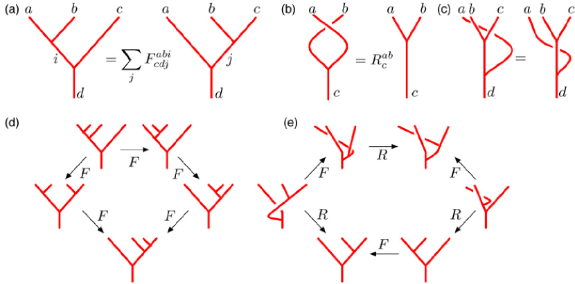
Figure 7: Rules for braiding and recoupling anyons. (a) Recoupling for a two-vertex interaction is obtained via a six index complex matrix $F$: the quantum $6-j$ symbol. (b) A braiding operation is related to an unbraid by the $R$ matrix. (c) The intertwining operation is topologically trivial. (d) The pentagon identity. Starting from a four vertex interaction, a sequence of five recouplings returns to the original interaction. It is taken as an axiom that this sequence is the identity mapping. (e) The hexagon identity relating three vertex interactions by a sequence of recoupling, intertwining, and braiding operations.

A comprehensive set of rules for manipulating anyons is given in Figure 7. These rules describe physically allowed operations on the state space. For example, one can braid the anyons before fusing them. This operation is described by the $R$ matrix and it is depicted in Figure 7(b). An additional evolution in the fusion space is possible by changing the order of fusion of three anyons. For example one can fuse the anyons $a$, $b$ and $c$ by two distinctive ways. One can first fuse $a$ with $b$ and then with $c$ or first fuse $b$ with $c$ and then with $a$. As shown in Figure 7(a), these two processes are related by a six index object $F$. This complex valued function is the $6-j$ symbol for quantum spin networks (Kauffman 1991):

$$F^{abi}_{cdj}=\left\{\begin{array}[]{ccc}a&b&j\\ c&d&i\end{array}\right\}_{q}.$$ (4)

Analogous to angular momentum recoupling, the $F^{abi}_{cdj}$ are physical, i.e. non-zero, only if the triples $\{abi\}$, $\{cdi\}$,$\{adj\}$,$\{cbi\}$ are allowed products under fusion. With the proper normalization, for each set of labels $(abcd)$ involved in a two vertex interaction, the matrix $F(abcd)^{i}_{j}$ is unitary. For the classical groups, the theory describes a gauge theory with gauge group $G$. For example, for $G=SU(2)$ the states are labelled by ascending half integers $\left|j/2\right\rangle$ and the branching rules for three indices $\{j_{1}j_{2}j\}$ satisfy the triangle inequality as given by the fusion rules: $j_{1}\times j_{2}=\oplus_{j=|j_{2}-j_{1}|}^{j_{1}+j_{2}}j$. Note that there is no upper bound on the magnitude of angular momentum, so the number of states on any edge is in principle infinite. For quantum groups, other possibilities exist. For example, for the Chern-Simons theory with gauge group $G=SU(2)_{k}$ the states are again labelled by ascending half integers but there is an upper bound $j\leq k/2$ and the fusion rule is modified so that $j_{1}+j_{2}+j\leq k$. Then the quantum $6-$j symbol in Eq. (4) is the $q-$deformed analogue of the classical $6-$j symbol with the value $q=e^{2\pi i/(k+2)}$. It parameterizes the deformation of the commutation relations for the algebra $\mathfrak{su}(2)$ viz. $[S^{z},S^{\pm}]=\pm S^{\pm},[S^{+},S^{-}]=\frac{q^{S^{z}}-q^{-S^{z}}}{q^{1/2}-q^{-1/2}}$.

From the pentagon rule, the following relation between the elements of the $F$ matrices is obtained:

$$\sum_{n}F(m\ell kp)^{q}_{n}F(jimn)^{p}_{s}F(js\ell k)^{n}_{r}=F(jiqk)^{p}_{r}F(rim\ell)^{q}_{s}.$$ (5)

Similarly, from the hexagon rule

$$R^{mk}_{r}F(\ell mkj)^{q}_{r}R^{m\ell}_{q}=\sum_{p}F(\ell kmj)^{p}_{r}R^{mp}_{j}F(m\ell kj)^{q}_{p}$$ (6)

These two polynomial equations must be solved to obtain a consistent set of $F$ and $R$ matrices. For example, from the fusion rules for Fibonacci anyons, one finds the non-zero values

$$\begin{array}[]{lll}F(1101)^{1}_{1}&=&F(0111)^{1}_{1}=F(1110)^{1}_{1}=F(1011)^{1}_{1}=1,\\ F(0000)^{0}_{0}&=&1,F(1111)=\left(\begin{array}[]{cc}\frac{1}{\phi}&\frac{1}{\sqrt{\phi}}\\ \frac{1}{\sqrt{\phi}}&-\frac{1}{\phi}\end{array}\right).\end{array}$$ (7)

These solutions are unique up to a choice of gauge.

Inserting these values into the relations demanded by the hexagon identity, one obtains the following $R$ matrix describing exchange of two particles:

$$R=\left(\begin{array}[]{cc}e^{4\pi i/5}&0\\ 0&-e^{2\pi i/5}\end{array}\right).$$ (8)

It can be shown that the unitaries $b_{1}=R$ and $b_{2}=F(1111)RF(1111)^{-1}$ acting in the logical space $\left|0\right\rangle$ and $\left|1\right\rangle$ are dense in $SU(2)$ in the sense that they can reproduce any element of $SU(2)$ with accuracy $\epsilon$ in a number of operations that scales like $O(poly(log(1/\epsilon))$ (Preskill 2004). Thus an arbitrary one qubit gate can be performed as follows: begin from the vacuum and prepare four anyons labelled $a_{1},a_{2},a_{3},a_{4}$. This is a subspace with total charge zero. Braiding the first and second anyons implements $b_{1}$ and braiding the second and third anyons implements $b_{2}$. A measurement of the outcome upon fusing $a_{1}$ and $a_{2}$ projects onto logical $\left|0\right\rangle$ or $\left|1\right\rangle$. Similarly, by performing braiding over $8$ anyons in state $1$, one obtains a dense subset of $SU(d(7))$. Since $SU(4)\subset SU(13)$, we can also implement any two logical qubit gate, e.g. the CNOT gate, with arbitrary accuracy. Hence the Fibonacci anyon model allows for universal computation on $n$ logical qubits using $4n$ physical anyons (Freedman et al. 2005).

5 A new quantum algorithm!

The study of anyonic systems for performing quantum computation has led to the exciting discovery of a new quantum algorithm that evaluates the Jones polynomials (Jones 1984). These polynomials are topological invariants of knots and links and they were first connected to topological quantum field theories by Witten (1989). Since then they have found far reaching applications in various areas such as in biology for DNA reconstruction or in statistical physics (Kauffman, 1991). The best know classical algorithm for the exact evaluation of Jones polynomials demands exponential resources (Jaeger, Vertigan, and Welsh, 1990). Employing anyons only a polynomial number of resources is required to produce an approximate answer of this problem (Freedman et al. 2003). The techniques used by manipulating anyons resemble more an analogue computer. Indeed, the idea is equivalent to the classical setup where a wire is wrapped several times around a solenoid that confines magnetic flux: by measuring the current that runs through the wire one can obtain the number of times the wire was wrapped around the solenoid. The translation of the corresponding anyonic evolution to a quantum algorithm was explicitly demonstrated by Aharonov, Jones and Landau (2005).

To better understand the structure of the computation, let us first introduce a few necessary elements. The main mathematical structure behind the evolution of anyons is the braid group $B_{n}$ on $n$ strands. Its elements $b_{i}$ for $i=1,...,n-1$ can be viewed as braiding the world lines of anyons. Specifically, if $n$ anyons are placed in a certain order then the element $b_{i}$ describes the effect of exchanging the position of anyons $i$ and $i+1$, e.g. in a counterclockwise fashion. Thus all possible manipulations between the anyons can be written as a combination of the $b_{i}$’s. The elements of the group $B_{n}$ satisfy the following relations

$$\left\{\begin{array}[]{cc}b_{i}b_{j}=b_{j}b_{i},&\text{for}\,\,\,|i-j|\geq 2\\ b_{i}b_{i+1}b_{i}=b_{i+1}b_{i}b_{i+1},&\text{for}\,\,\,1\leq i<n\end{array}\right.$$

These relations have a simple geometrical meaning, as presented in Figure 8. Note that the symmetric group $S_{n}$ is a representation of $B_{n}$ if we impose the condition that $b_{j}^{2}=1,\,\,\forall j$. This would be true for boson and fermions where $b_{j}=\pm 1$ but, as discussed earlier, in two dimensions other possibilities exist.

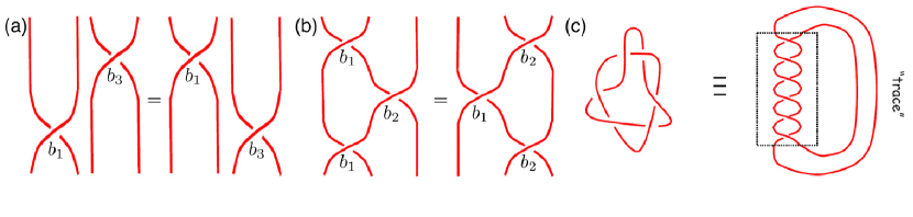
Figure 8: Connection between braids and knots. (a) Schematic representation of the relation $b_{i}b_{j}=b_{j}b_{i}$ when $|i-j|\geq 2$. Exchanging the order of two braids does not have an effect if they are sufficiently far apart. (b) Schematic representation of the relation $b_{i}b_{i+1}b_{i}=b_{i+1}b_{i}b_{i+1}$ for $1\leq i<n$. The two braidings are equivalent under simple continuous deformations. (c) The Markov trace performed by linking the opposite ends of the strands. It creates out of the six braidings a link between two strands.

The second element we need for the quantum algorithm is the introduction of a trace that will establish the equivalence between braidings and knots or links. A version of this tracing procedure called the Markov trace consists of connecting the opposite endpoints of the braids together as shown in Figure 8(c). Thus, any braid with a trace gives a knot or a link. Surprisingly, every knot or link is equivalent to a braid with a trace as is demonstrated by Alexander’s theorem (Alexander 1923). Hence, one can simulate a knot or a link by braiding anyons.

The general idea for relating a polynomial in a complex variable to a certain knot or link is as follows. We first need to consider a single braid and relate to it a linear combination of two other diagrams, as depicted in Figure 9(a).

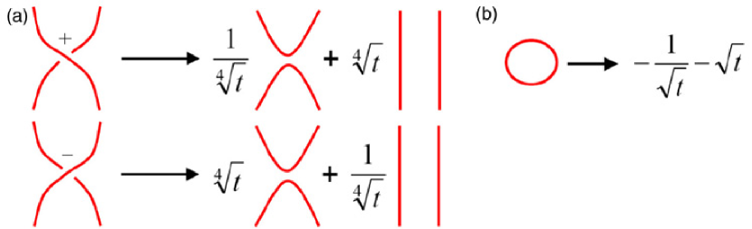
Figure 9: Skein relations for disentangling knots. (a) Each braid is smoothed according to a linear combination of the avoiding strands and the identity strands. The crossing sign $\pm$ of a braid determines its decomposition into unbraids. (b) A closed loop contributes a complex number.

The coefficients are a function of the complex parameter $t$ that is the variable of the Jones polynomials. This step, together with the tracing, produces a number of closed loops that are not linked to each other. To each closed loop the complex number $d=-\sqrt{t}^{-1}-\sqrt{t}$ is attributed, as seen in Figure 9(b). These procedures are enough to associate a Laurent polynomial with each knot or link, and subsequently to each traced braid.

Specifically, the Jones polynomial is defined by

$$J_{K}(t)=\Big{(}-\frac{1}{\sqrt[4]{t}}\Big{)}^{-w(K)}\langle K\rangle(t)$$ (9)

Here $w(K)$ is the writhe of the knot $K$ which is defined as the sum of the crossing signs (as defined in figure 9(a)) and the Kauffman bracket of $K$ is defined by

$$\langle K\rangle(t)=\sum_{S}\langle K\left|S\right\rangle d^{L(S)-1}$$ (10)

where $S$ is a choice of smoothings for each crossing of $K$ and $L(S)$ is the number of loops in the state $S$. There are two choices of smoothing per crossing so the total number of states is $2^{N}$ for a knot with $N$ crossings. The product of the weights $\frac{1}{\sqrt[4]{t}}$ and $\sqrt[4]{t}$ over all the crossings for a particular state $S$ is $\langle K\left|S\right\rangle$.

The Jones polynomial has been shown to be a topological invariant (Jones 1984), i.e its value for a given knot $K$ is unchanged under continuous deformations. For two knots $K_{1}$ and $K_{2}$, if $J_{K_{1}}\neq J_{K_{2}}$ then $K_{1}$ and $K_{2}$ are inequivalent, i.e. they cannot be mapped to each other by continuous deformations. Note, however, that inequivalent knots may have the same Jones polynomial. Computation of the Jones polynomial by a classical computer appears to be exponentially hard due to the fact that there are exponentially many terms to sum and no closed form for the number of loops as a function of the resolution of the knot exists. On the other hand it is rather easy to calculate its value with the anyons.

For illustration we sketch the quantum algorithm that evaluates the Jones polynomial for the three strand braid group $B_{3}$ (see also Kauffman and Lomonaco (2006)). First one picks a representation of the braid group. A one dimensional unitary representation is given by $b_{j}=e^{i\phi},\,\,\forall j$ which describes exchange of identical particles with abelian anyonic statistics. The simplest non-abelian representation is given by $2\times 2$ matrices which can be parameterized as: $\Gamma(b_{j})=\frac{1}{\sqrt[4]{t}}{\bf 1}_{2}+\sqrt[4]{t}V_{j}$ where

$$V_{1}=\left(\begin{array}[]{cc}d&0\\ 0&0\end{array}\right),\quad V_{2}=\left(\begin{array}[]{cc}d^{-1}&\sqrt{1-d^{-2}}\\ \sqrt{1-d^{-2}}&d-d^{-1}\end{array}\right),$$ (11)

in which case $\Gamma(b_{1})\Gamma(b_{2})\Gamma(b_{1})=\Gamma(b_{2})\Gamma(b_{1})\Gamma(b_{2})$. The set $\{{\bf 1}_{2},V_{1},V_{2},V_{1}V_{2},V_{2}V_{1}\}$ generates what is known as a Temperley-Lieb algebra and satisfies $V_{1}V_{2}V_{1}=V_{1}$, $V_{2}V_{1}V_{2}=V_{2}$. The representation becomes unitary if we choose $t=e^{-i\theta}$ for $|\theta|\leq 2\pi/3$ or $|\theta/4+\pi|\leq\pi/6$. Any sequence of $k$ braids can be described by a braid word $r=r_{1}r_{2}\ldots r_{k}$ and this word has a closure which corresponds to a knot $K_{r}$. For $B_{3}$ we have $r_{k}\in\{b_{1},b_{2}\}$ so $\langle K_{r}\rangle=\langle\prod_{j=1}^{k}\Gamma(r_{j})\rangle=\langle(1/\sqrt[4]{t})^{k}{\bf 1}_{2}\rangle+\langle F(r)\rangle$, where $F(r)$ is a sum of products of the matrices $V_{1},V_{2}$. A closed loop composed with a knot $K$ has a bracket that is $d$ times that of $\langle K\rangle$ and the bracket of one closed loop is $1$. Hence, the closure of the identity operation on $B_{3}$ represents three closed loops and $\langle{\bf 1}_{2}\rangle=d^{2}$. The bracket of the closure of a braid word is a function computed by taking the trace over the carrier space of the representation and we have $\langle K_{r}\rangle(t)=(\frac{1}{\sqrt[4]{t}})^{k}(d^{2}-2)+\mbox{Tr}[\prod_{j=1}^{k}\Gamma(r_{j})]$. The difficulty of computing the Jones polynomial is then reduced to computing the trace of a product of unitaries.

Good quantum algorithms exist for computing traces of unitaries. For example, one can begin with a completely mixed state of $n$ register qubits and one work qubit $w$ prepared in the pure state $(\left|0\right\rangle_{w}+\left|1\right\rangle_{w})/\sqrt{2}$. Applying a sequence of controlled unitaries $\prod_{j=1}^{k}\left|1\right\rangle_{w}{{}_{w}}\left\langle 1\right|\otimes\Gamma(r_{j})$ and measuring the work qubit in the $\hat{x}$ and $\hat{y}$ bases outputs the real and imaginary parts of the normalized trace $\mbox{Tr}[\prod_{j=1}^{k}\Gamma(r_{j})]/2^{n}$. The unnormalized expectation value of a unitary in a particular state $\left|s\right\rangle$ can be computing by replacing the mixed state with the pure state $\left|s\right\rangle$. For the $U(2)$ representation of $B_{3}$ above, one register qubit suffices and in fact there is no need to have a physical system with anyons. More complicated braids over different unitary representations can be computed by performing the controlled unitary gates using several qubits in the quantum circuit model, or by implementing the operations by physical braiding of anyons. By direct measurement of the anyons it is possible to determine the value of the Jones polynomial. The measurement of the anyonic state can be performed by an interference experiment as discussed below. The algorithmic translation of this process (Aharonov, Jones and Landau 2005) provides a quantum algorithm that can obtain the value of the Jones polynomials for general $t$.

6 Realizations of anyons

6.1 Quantum Hall Effect

Several candidates for physical realizations of particles with anyonic properties exist. Historically, it was first suggested that the elementary charged excitations of a fractional quantum Hall (FQH) fluid should obey fractional statistics (Halperin 1984, Arovas, Schrieffer and Wilczek 1984). In the quantum Hall effect, a 2D electron gas (electron charge $q_{e}$ and density $n$) moves under the influence of a magnetic field ${\bf B}$ normal to the plane and an electric field ${\bf E}$ in the plane. By the Lorentz force a current is induced perpendicular to ${\bf E}$. Classically, the resistance varies inversely with $\nu=nhc/q_{e}|{\bf B}|$, but in the presence of strong magnetic fields, plateaus in the Hall resistance occur at integer, as well at some fractional values, of the filling $\nu$. These plateaus of quantized resistance indicate where the 2D electron gas acts as an incompressible fluid, meaning that all charged excitations have a finite energy gap. Disorder plays an important role in localizing the charge excitations, this creates a mobility gap against delocalized charged excitations which would contribute to transport.

There is a fundamental difference in the low energy physics between the integer and fractional filling cases. For integer $\nu$ the gap can be understood without electron interactions because each plateau corresponds to a completely filled Landau level and incompressibility follows by the Pauli exclusion principle. However, for fractional filling, the energy gap can only be explained by including interactions, i.e. the excitations are a collective phenomenon. Laughlin found a trial wavefunction for the FQHE at $\nu=1/m$ for $m$ odd given by

$$\psi_{m}=\prod_{j<k}(z_{j}-z_{k})^{m}e^{-\sum_{i}|z_{i}|^{2}/4\ell_{B}^{2}}$$ (12)

where $\{z_{i}\}$ are the complex electron coordinates in the plane and $\ell_{B}=|c\hbar/q_{e}B|$ is the magnetic length (Laughlin 1983). The fractionalization of the charge follows by considering a quasihole excitation at position $\zeta$ above the ground state $\psi_{m}$:

$$\phi^{h}(\zeta,\zeta^{*})\propto\prod_{i}(\zeta-z_{i})\psi_{m}$$ (13)

The appropriate charge value is obtained by removing an electron from the ground state $\psi_{m}$ producing the wavefunction $\prod_{i}(\zeta-z_{i})^{m}\psi_{m}$. This state can be viewed either as a charge $e$ hole at position $\zeta$ or as $m$ quasiholes at position $\zeta$. Hence the quasihole charge is $e/m$ and there is an associated qausiparticle excitation with charge $-e/m$ (see e.g. Wen 2004). More generically, quasiparticles can be viewed as composite fermions in a FQH condensate at filling $\nu=p/(2jp+1)$ for $j,p\in\mathbb{N}$ that carry charge $q=e/(2jp+1)$ (Jain 1989).

One way to compute the fractional statistics is to wind a charge $q$ quasiparticle at position ${\bf r}_{1}$ around a closed path $\Gamma$ containing another charge $q$ quasiparticle at position ${\bf r}_{2}$ in the $\nu$ filled FQH state. The Berry’s phase thus accumulated is

$$\gamma=i\oint_{\Gamma}d{\bf r}_{1}\langle\psi({\bf r}_{1},{\bf r}_{2})|\bigtriangledown_{{\bf r}_{1}}\psi({\bf r}_{1},{\bf r}_{2})\rangle.$$ (14)

This quantity can be explicitly calculated by considering a time dependent potential $V({\bf r}-{\bf r}_{1}(t))$ which localizes particle $1$ and allows for adiabatic braiding around particle $2$. Subtracting off the phase accumulated when no particle exists inside $\Gamma$ the relative statistical phase is (Arovas, Schrieffer and Wilczek 1984)

$$\phi_{p/(2jp+1)}^{p/(2jp+1)}=\delta\gamma/2\pi=2j/(2jp+1).$$ (15)

Theory predicts non-abelian anyons occur in FQH at special filling fractions. This startling discovery was originally made for the $\nu=5/2$ state by Moore and Read (1991) and subsequent work predicted non-abelian anyons at other filling fractions such as $\nu=12/5$ (Read and Rezayi, 1999). In the later case, the quasiparticles transform under a quantum group sufficiently rich to support fault tolerant universal quantum computation (Freedman et al. 2003). The more experimentally accessible and stable $\nu=5/2$ state is shown in the Moore-Read model to have nonabelian composite particles. These anyons have computational power that is not strictly fault tolerant but can be made so with some amount of non-topologically protected preparation steps (Bravyi 2006). The braiding properties of the $\nu=5/2$ and $\nu=12/5$ quasiparticles were derived by Nayak and Wilczek (1996) and Bais and Slingerland (2001). While there is strong theoretical support for the existence of non-abelian anyons in these systems, a definitive experimental demonstration of the fact is still an active pursuit.

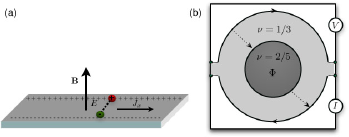
Figure 10: Fractional Quantum Hall fluid. (a) Schematic of a 2D electron gas with a current ${\bf J}$ induced perpendicular to an electric field ${\bf E}$ and a strong magnetic field ${\bf B}$. (b) Experimental setup to observe anyonic statistics. The system consists of a $\nu=1/3$ fluid surrounding a $\nu=2/5$ island. Current carrying $e/3$ quasiparticles can tunnel between inner and outer $1/3$ edges changing the potential from $V=0$ to $V>0$. Current along the closed path on the inner edge gives rise to oscillations in the conductance as a function of the enclosed flux $\Phi$ due to the Aharonov-Bohm effect. The presence of charge $e/5$ particles in the island affects the phase of the circulated particles which is observed the interference pattern in the conductance.

6.2 Lattice Models

In Sec. 3 we saw that a Hamiltonian whose ground states comprise a surface code have excited states which behave like abelian anyons. It is also possible to rig spin lattice models with non-abelian excitations. In one type of construction (Kitaev 2003; Doucot and Ioffe 2005), each spin is endowed with a state space whose dimension is equal to the order of a discrete non-abelian group $G$. The vertex and face interactions can then be constructed as appropriate sums over products of Hopf algebra elements acting on $G$ such that the ground states are invariant under local non-abelian gauge transformations and the excitations are massive non-abelian quasiparticles.

There are other systematic ways to construct spin lattice models , that directly encode the fusion rules of emergent anyons (Turaev and O. Y. Viro 1992; Fendley and Fradkin 2005; Freedman et al. 2004). One such construction, known as the string net model (Levin and Wen 2005; Fidkowski et al., 2006), involves spins with short ranged interactions and low energy states that enforce rules for branching and reconnecting loops of string on a background lattice. In the model of Levin and Wen, the interactions take place amoung qudits that reside on the oriented edges of a honeycomb lattice. Here the $d$ states of each particle correspond to the vacuum plus $d-1$ string types that enumerate the irreducible representations of a group $G$. The orientation of the string relative to the edge orientation determines whether the string is of type $s$ or its dual $s^{\ast}$. For simplicity, we discuss only the case for self dual strings. As with the surface code construction, the Hamiltonian can be expressed as a sum of commuting vertex and face operators:

$$H=-U\sum_{v}H_{v}-J\sum_{f}H_{f}.$$ (16)

Here, the vertex interaction encodes the appropriate fusion rules for the anyons

$$H_{v}=\sum_{i,j,k=0}^{d-1}\left|\{ijk\}\right\rangle\left\langle\{ijk\}\right|$$ (17)

where $\{ijk\}$ represents an allowed branching of the strings. The operator is diagonal in the spin basis $\{\left|k\right\rangle\}_{s=0}^{d-1}$ and contains terms like $\left|ijk\right\rangle\left\langle ijk\right|$ indicating that if the oriented edges meet at a vertex $v$ then the allowed fusion products are $i\times j\rightarrow k,i\times k\rightarrow j,j\times k\rightarrow i$. The face constraints contain information about the action on the state space under fusion of string types on the boundary of a face. It can be thought of as the closure of Figure 6(a) where the horizontal edges correspond to edges on the boundary of a hexagon and the vertical edges emanate from the hexagon, viz :

$$H_{f}=\frac{1}{\sum_{s}d_{s}^{2}}\sum_{s=0}^{d-1}d_{s}B^{s}_{f},$$ (18)

where $d_{s}$ is the quantum dimension of the particle type $s$. The operators $B^{s}_{f}$ are $12$-local operators that encode the gauge invariance of the theory with appropriate weighting by the recoupling matrices $F(ijk\ell)$. As with the surface codes, there are a set of $N$ closed string types which commute with the Hamiltonian $H$. The ends of various types of open strings correspond to quasi-particles with appropriate statistics.

Let us consider how the spin model gives rise to Fibonacci anyons. As discussed above, this theory has two particle types: $1$ and $0$ with the fusion rule $1\times 1=0+1$. We recover this rule if we consider the Chern-Simons theory $SU(2)_{3}$ but exclude non-integer state labels. The resulting theory with two particle types is also known as $SO(3)_{3}$. The two particle types are represented as string types on the edges of the honeycomb lattice: the vacuum (or empty particle) state $\left|0\right\rangle_{e}$ and single particle state $\left|1\right\rangle_{e}$. The low energy subspace is spanned by states that satisfy the constraints

$$\begin{array}[]{lll}H_{v}&=&\left|111\right\rangle\left\langle 111\right|+\left|011\right\rangle\left\langle 011\right|+\left|101\right\rangle\left\langle 101\right|+\left|110\right\rangle\left\langle 110\right|+\left|000\right\rangle\left\langle 000\right|\\ &=&-\sum_{j=1}^{3}Z_{e_{j}}+Z_{e_{1}}Z_{e_{2}}+Z_{e_{1}}Z_{e_{3}}+Z_{e_{2}}Z_{e_{3}}+3Z_{e_{1}}Z_{e_{2}}Z_{e_{3}}.\end{array}$$ (19)

Here the quantum dimensions are $d_{0}=1$ and $d_{1}=(1+\sqrt{5})/2$, and the explicit form for the face operators is

$$\begin{array}[]{lll}B^{0}_{f}&=&\displaystyle{\sum_{r\in\{0,1\}}}\left|rrrrrr\right\rangle\left\langle rrrrrr\right|\otimes\left|rrrrrr\right\rangle{{}_{\hexagon}}{{}_{\hexagon}\left\langle rrrrrr\right|}\\ B^{1}_{f}&=&\displaystyle{\sum_{a,b,c,d,e,f\in\{0,1\}}}\left|abcdef\right\rangle\left\langle abcdef\right|\otimes\displaystyle{\sum_{\begin{subarray}{c}g,h,i,j,k,\ell,g^{\prime},h^{\prime},\\ i^{\prime},j^{\prime},k^{\prime},\ell^{\prime}\in\{0,1\}\end{subarray}}}\left|g^{\prime}h^{\prime}i^{\prime}j^{\prime}k^{\prime}\ell^{\prime}\right\rangle{{}_{\hexagon}}{{}_{\hexagon}\left\langle ghijk\ell\right|}\\ &&F(a\ell 1g^{\prime})^{g}_{\ell^{\prime}}F(bg1h^{\prime})^{h}_{g^{\prime}}F(ch1i^{\prime})^{i}_{h^{\prime}}F(di1j^{\prime})^{j}_{i^{\prime}}F(ej1k^{\prime})^{k}_{j^{\prime}}F(fk1\ell^{\prime})^{\ell}_{k^{\prime}}\\ &&\end{array}$$ (20)

where the $F$ matrices are as derived above. Notice that $B^{s}_{f}$ is block diagonal in the basis of the edge qubits that eminate from the hexagon (see Figure 11). The operator of $B^{s}_{f}$ can be obtained constructively by deriving the transition matrix between one string configuration around a face that is fused with a virtual $s$ type string inside to produce another valid string configuration around the face.

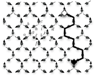
Figure 11: A spin lattice model admitting non-abelian anyons. Here the particles reside on Kagomé lattice and can be identified with oriented edges of a honeycomb lattice. The particles each have $N$ states enumerating the irreducible representations of a group $G$. The states can be thought of as labelling a string type and the Hamiltonian commutes with closed strings of a given type. The anyons of type $s$ exist as ends of open strings (thick black line) of the same type. Three body interactions at a vertex encode the fusion rules, e.g. the particle state $\left|ag\ell\right\rangle$ is in the span of low energy states if any pair of those indices can combine to give the third. The face operators encode the recoupling under the $F$ matrices of the twelve particles around a face, e.g. $\{abcdefghijk\ell\}$.

The string net picture is a beautiful illustration of a microscopic model that realizes topological phases. A major stumbling block is that it requires a Hamiltonian that includes $12$-body interaction terms, i.e. it is $12$-local, making a physical realization of such a model implausible. Nature tends to favor binary interactions and it would be helpful to have a microscopic spin model with emergent anyons that involved $2$-local interactions only. In such a case, one could imagine engineering interactions in the laboratory using fields to coherently couple quantum mechanical spins in the desired manner. Yet most spin lattice models with emegent anyons require at least $4$-local interactions on a 2D lattice.. How is one to achieve a quantum simulation of such models? One possible resolution is to obtain the $k$-local interaction as an effective model in perturbation theory. Another possibility is to use ancillary particles to mediate the $k$-local interaction (Oliveira and Terhal 2004). The caveats to both these approaches are: first, the effective Hamiltonians in the ground states that approximate the model Hamiltonian occur only at high order in perturbation theory and hence have a small coupling strength or require energy gaps in the ancillae which scale with the system size, and second, the microscopic interactions are highly anisotropic in spatial and spin degrees of freedom.

One $2$-local spin model that does have anyonic excitations is the following anisotropic interaction on a honeycomb lattice (see Figure 12)

$$H_{\rm hc}=-J_{x}\sum_{x-{\rm links}}X_{i}X_{j}-J_{y}\sum_{y-{\rm links}}Y_{i}Y_{j}-J_{z}\sum_{z-{\rm links}}Z_{i}Z_{j}.$$ (21)

This model is exactly solvable (Kitaev 2006; Pachos 2006) and has two distinct phases. When the couplings satisfy the triangle inequalities $|J_{x}|\leq|J_{y}|+|J_{z}|,|J_{y}|\leq|J_{x}|+|J_{z}|,|J_{z}|\leq|J_{x}|+|J_{y}|$ then the system is gapless, but it becomes gapped in the presence of a magnetic field and has non-abelian anyonic excitations. Otherwise, the system is gapped and for the case where one of the couplings is much greater than the others, the excitations are described by abelian anyons in a $\mathbb{Z}_{2}$ gauge theory. Recently, two physical constructions of this model were proposed using atomic (Duan, Demler and Lukin 2003) and molecular arrays (Micheli, Brennen, and Zoller 2006). Both proposals involving trapping of the particles, one per well, in an optical lattice which is a periodic potential produced by interfering standing waves of laser light. Spin is encoded in internal hyperfine states and the particles interact either by nearest neighbor spin dependent collisions or by field induced dipole-dipole interactions (see Figure 12).

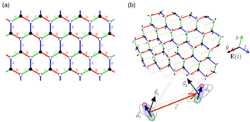
Figure 12: A honeycomb spin lattice model due to Kitaev which has anyonic excitations. (a) The coupling graph depicted on a plane. The lattice is bipartite with physical qubits indicated by black and white dots and the color of the links indicating the anisotropy of the interaction. (b) Proposed realization using polar molecules trapped in an optical lattice. The spin corresponds to a single valence electron of an alkaline earth monohalides. The molecules are prepared in rovibrational ground states and trapped one molecule per lattice well with nearest neighbor spacing $\lambda/2$ where $\lambda$ is an optical wavelength. The molecules are made to interact using microwave fields ${\bf E}(t)$ which induce dipole-dipole interactions. For a judicious choice of microwave frequencies, polarizations, and intensities, the effective interaction in the ground states between two molecules separated by ${\bf r}=r\hat{r}$ is $C(r)\vec{\sigma}\cdot\hat{r}\otimes\vec{\sigma}\cdot\hat{r}$, where $C(r)$ is a function that is large near microwave resonance at $r=\lambda/2$ but decays rapidly beyond this separation. The appropriate terms in $H_{\rm hc}$ are achieved when nearest neighbors form orthogonal triads along $\hat{x},\hat{y},\hat{z}$ in real space. This is engineered by trapping the molecules in two staggered triangular optical lattices such that the nearest neighbor coupling graph is a honeycomb lattice.

7 Observation of anyons

The signature of anyonic properties is their nontrivial evolution under braiding and this behavior can be probed via interference measurements. Quite recently, an interferometer type experiment with quasiparticles in a FQH fluid found evidence supporting abelian anyonic statistics (Camino, Zhou and Goldman 2005). In that experiment, a quasiparticle with charge $e/3$ in a $\nu=1/3$ FQH fluid makes a closed path trajectory around an island of $\nu=2/5$ FQH fluid (see Figure 10b) and the relative statistics are probed. Interference fringes manifest as peaks in the conductance as a function of the magnetic flux through the $\nu=2/5$ island. The experiment observed periodic modulation consistent with the excitation of ten $q=e/5$ quasiparticles in the island fluid. Adapting the Berry’s phase argument for encircling several quasiparticles (Jain 1993), this evidence then implies a relative statistics of $\phi_{2/5}^{1/3}=-1/15$ when a charge $e/3$ quasiparticle encircles one $e/5$ quasiparticle of the $\nu=2/5$ filled fluid. Nevertheless, the unambiguous detection of anyons is still considered an open issue (Kim, 2006; Rosenow and Halperin 2007).

Several new theoretical proposals have been made for observing non-abelian statistics in FQH states (see e.g. Das Sarma, Freedman, and Nayak 2005; Stern and Halperin 2006; Bonderson, Kitaev and Shtengel 2006; Bonderson, Shtengel, and Slingerland 2007). Ironically, experimental signature of the non-abelian anyons may be more robust than the abelian case. Indeed, in the abelian case the braiding results in phase factors that are both geometrical and dynamical in nature and thus hard to distinguish. To the contrary, the non-abelian anyons cause a change in the amplitude of the participating states which is easily distinguished from spurious dynamical phase factors.

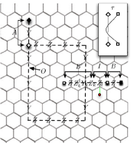
Figure 13: Interferometer for measuring statistics of abelian anyons. The system is the gapped phase of the honeycomb mode $H_{\rm hc}$. The inset illustrates the braiding of a flux around a charge. The steps are as follows: (1) beginning in the vacuum state $\left|\lambda_{g}\right\rangle$ prepare a charge anti-charge pair in region $A$ and a flux anti-flux pair in region $B$. (2) Apply the “beam splitter” operation $e^{-i\frac{\pi}{4}Z_{\ell}}$ in region $I$; this creates a delocalized state of the flux $\square$. (3) Adiabatically drag the flux particle left along the trajectory $B^{\prime}$. (4) Adiabatically drag the charge particle $\diamond$ counterclockwise around the flux along the path $O$. (5) Adiabatically drag the flux right along $B^{\prime}$. (5) Apply the inverse beam splitter operation $e^{i\frac{\pi}{4}Z_{\ell}}$. (6) Measure the location of the flux, i.e. measure $\langle Z_{\ell}\rangle=\sin(\beta+\phi^{1}_{1})$. Here $\beta$ is the accumulated dynamical and Berry’s phases and $\phi^{1}_{1}$ is the mutual statistics of the charge and flux. (7) Repeat the above steps in the order $(1,2,4,3,5,6)$ such that the braid is trivial and $\langle Z_{\ell}\rangle=\sin(\beta)$. It is then possible to extract $\phi^{1}_{1}$ which is equal to $\pi$.

It should also be possible to observe anyonic statistics in spin lattice realization. As an example consider the honeycomb model $H_{\rm hc}$ in the regime where $|J_{z}|\gg|J_{x}|,|J_{y}|$. In the low energy sector, each pair of spins $e_{1},e_{2}$ on a $z-$link gets mapped to an effective two level system. The $\mathfrak{su}(2)$ algebra for each spin is spanned by the two body operators $\tilde{Z}_{e}=Z_{e_{1}}$, $\tilde{X}_{e}=X_{e_{1}}X_{e_{2}}$, $\tilde{Y}_{e}=Y_{e_{1}}X_{e_{2}}$. In perturbation theory to fourth order in $|J_{\perp}/J_{z}|$, the effective Hamiltonian in the ground states is then (Kitaev 2003)

$$H_{\rm eff}=-J_{\rm eff}\sum_{\diamond}\tilde{Y}_{\rm left}\tilde{Z}_{\rm up}\tilde{Y}_{\rm right}\tilde{Z}_{\rm down}$$ (22)

where $J_{\rm eff}=J_{x}^{2}J_{y}^{2}/16|J_{z}|^{3}$ and the operator subscripts indicate the location of the $z-$links which are at the corners of a diamond. This model was first introduced by Wen (2003) and is locally equivalent to the surface code Hamiltonian of Eq. (3). Here flux anti-flux pairs are created on the left and right of a $z-$link $e$ by applying $Z_{e}$ to the vacuum. Charge anti-charge pairs are created above and below $e$ by applying $Y_{e}$. Dyonic combinations are created by applying $X_{e}$. The mass of each particle is $J_{\rm eff}$. In Figure 13 we sketch an interferometer type experiment to extract the mutual statistics of anyonic charge and flux. The particles are braided adiabatically along non-contractible loops. Adiabatic motion could be achieved by modifying the Hamiltonian such that $H^{\prime}(t)=H_{\rm hc}+\sum_{e\in Path}\delta J_{e}(t)Z_{e_{1}}Z_{e_{2}}+\kappa(t)Z_{e}(t)$. For a properly tuned $\delta J_{e}(t)$ this creates a reduced effective mass for the particle along the trajectory and hence makes it energetically favorable to follow the intended path. Such a protocol could be implemented with atoms or molecules trapped in an optical lattice provided one had single lattice site addressability. This can be accomplished in principle with gradient field spectroscopy using lasers with shaped intensity profiles (Zhang, Rolston and Das Sarma 2006).

8 Criteria for TQO and TQC

Clearly there is need for many technological advances in order to realize experimentally topological order and topological quantum computation. Topological order corresponds to the property of long range correlations (or long range coherence). This is best captured by the concept of topological entropy (Hamma, Ionicioiu, and Zanardi 2005; Kitaev and Preskill 2006; Levin and Wen 2006) given by $S_{\rm{topo}}=\log D$ where $D=\sqrt{\sum_{j}d_{j}^{2}}$ is the total quantum dimension. The latter is non-zero only when there exists a loop operator defined on the two dimensional system that has a non-zero expectation value when the size of the loop is arbitrarily increased. Note, however, that there is some debate about whether topological entropy is a necessary and sufficient criterion for topological order (Nussinov and Ortiz, 2007). For the case of topological quantum computation, one should be able to bring a system in such a phase, then create anyons, braid them and finally measure them. This is a hard task and it is still not clear which technology will serve best to perform all these steps. For that we would like to introduce a list of criteria a physical system has to satisfy to be able to support TQO and which supplementary ones we have to use to be able to perform TQC.

Here is a list of criteria a system has to satisfy in order to be able to support TQO. In particular we will focus on a lattice system of qubits or qudits defined in two dimensions. Keep in mind that, to a large degree, the required steps depend on the particular topological theory one wants to realize and on the particular employed physical system.

• Initialization (Creation of highly entangled state)

• Addressability of qubits (Anyon generation and manipulation)

• Measurement (Entropic study of the ground state or interference of anyons)

• Scalability (Large systems)

• Low decoherence (Protected encoding subspace)

These criteria are required for the following reason:

• It should be possible to create a highly entangled state between all of the qubits of the system that has $S_{\rm{topo}}\neq 0$. It can be created either by a coherent process (dynamical preparation, adiabatic evolution) or a dissipative process such as a cooling mechanism.

• To create and manipulate anyons one has to be able to address the qubits of the system and perform local, possibly multiqubit, operations. Creation of anyons is a classical process and should be possible to happen in finite time.

• One should be able to measure the type (or color) of anyons by a suitable interference process. There are several ways this might be done including but not limited to: guiding individual quasiparticles along braiding paths as described in Sec. 7, weaving global string operators to measure the action on degenerate ground states, and braiding large defects (holes) followed by a measurement of the outcome under fusion.

• The system has to be sufficient large to be able to support the presence of several anyons and to perform braidings between them.

• The system should be sufficiently isolated from the environment or the temperature should be low enough compared to the energy gap so that the topological properties of the ground state or the statistical properties of the anyons can be read.

Requirements for protected topological phase and computation. These strongly depend on the employed physical system.

• The presence of a Hamiltonian that has the highly entangled state as its ground state and creates an energy gap above it that protects it from small perturbations.

• Trapping of anyons with local potentials (caused with external classical fields) that facilitate their generations at a certain point. Subsequently anyons should be able to be moved adiabatically to perform braiding (only one of them is necessary). If anyons move outside of trapping potentials then decoherence (error) may occur.

• Addressability of the different energy levels may be necessary for identifying anyons.

We emphasize that the above set of criteria is a helpful guide but may prove to be overly restrictive for a more general class of models with topological order. For example, it has been found that universal quantum computation is possible using only ground state manipulation, i.e. without quasiparticle braiding, using brane-net condensates in three dimensional spin lattices (Bombin and Martin-Delgado 2006). Furthermore, the possibility to perform global operations on finite sized systems may obviate the need to address excited states.

9 Conclusions

Topological quantum computation offers a rich arena for exciting developments in theoretical and experimental physics. It has created a new playground with unique links between information theory, physics and mathematics. Research in this area has proven already fruitful for quantum information and fundamental sciences and we expect to witness exciting developments in the near future. In this article we have reviewed some of the fascinating recent developments in this field, emphasizing the fundamental connection between physics and topology. An in depth study of the involved concepts and techniques can be found in the provided bibliography and in references therein.

References

- [1]
- [2] Aharonov, Y. and Bohm, D. 1959 Phys. Rev. 115, 485-491.
- [3] Alexander, J.W. 1923, Proc. Nat. Acad. Sci., 9, 93-95.
- [4] Arovas, D. Schrieffer, J.R., Wilczek, F. 1984, Phys. Rev. Lett. 53 722-723.
- [5] Aharonov, D. Jones, V. Landau, Z. 2005, quant-ph/0511096.
- [6] Bais, S. and Slingerland, J. 2001, Nucl. Phys. B 612, 229-290.
- [7] Bombin, H. and Martin-Delgado, M.A. 2007, Phys. Rev. Lett. 98, 160502.
- [8] Bonderson, P. Kitaev, A. and Shtengel, K. 2006, Phys. Rev. Lett. 96, 016803.
- [9] Bonderson, P, Shtengel, K., and Slingerland, J.K. 2006, Phys. Rev. Lett. 97, 016401.
- [10] Bonesteel, N.E., Hormozi, L., Zikos, G., and Simon, S.S. 2005, Phys. Rev. Lett. 95, 140503.
- [11] Bravyi, S 2006, Phys. Rev. A 73, 042313.
- [12] Bullock, S. and Brennen, G.K. 2007, J. Phys. A: Math. Theor. 40, 3481-3505.
- [13] Camino, F.E., Zhou, W. and Goldman, V.J. 2005, Phys. Rev. B 72, 075342-075349.
- [14] Das Sarma, S., Freedman, M., and Nayak, C. 2005, Phys. Rev. Lett. 94 ,166802.
- [15] Duan, L.M. , Demler, E. and Lukin, M.D. 2003, Phys. Rev. Lett. 91, 090402.
- [16] Doucot, B., and Ioffe 2005, L.B. New J. Phys. 7, 197, 1-30.
- [17] Farhi, E. Goldstone, J., Gutmann, S. Lapan, J., Lundgren, A., and Preda, D. 2001, Science 292, 472-475.
- [18] Fendley, P. and Fradkin, E. 2005, Phys. Rev. B 72, 024412-024430.
- [19] Fidkowski, L., Freedman, M., Nayak, C. Walker, K., Wang, Z. 2006, cond-mat/0610583.
- [20] Freedman, M.H., Larsen, M.J., and Wang, Z. 2002, Comm. Math. Phys. 227, 605-622; Freedman, M.H., Larsen, M.J., and Wang, Z. 2002, ibid, 228, 177-199.
- [21] Freedman, M. H., Kitaev, A. Larsen, M. J., and Wang, Z. 2003, Bull. Amer. Math. Soc. 40, 31-38.
- [22] Freedman, M.H., Nayak, C., and Shtengel, K. 2005, Phys. Rev. Lett. 94, 066401; cond-mat/0309120.
- [23] Freedman, M., Nayak, C. Shtengel, K., Walker, K., and Wang, Z. 2004 Ann. Phys. 310, 428-492.
- [24] Halperin, B.I. 1984, Phys. Rev. Lett. 52, 1583-1586.
- [25] Hamma, A., Ionicioiu, R. and Zanardi 2005, Phys. Rev. A 71, 022315.
- [26] Jaeger, F., Vertigan, D.L., and Welsh, D.J.A. 1990 Math. Proc. Cambridge Phil. Soc. 108, 35-53.
- [27] Jain, J.K. 1989, Phys. Rev. Lett. 63, 199-202.
- [28] Jain, J.K. 1993, Phys. Rev. Lett. 71, 3003-3006.
- [29] Jones, V. F. R. 1985, Bull. Amer. Math. Soc. 12, 103-111.
- [30] Kauffman, L.H. 1991, Knots and Physics World Scientific, Singapore.
- [31] Kauffman, L.H. and Lomanaco, S., 2006, quant-ph/ 0606114.
- [32] Kim, E-A. 2006, Phys. Rev. Lett. 97, 216404.
- [33] Kitaev, A. Yu. 2003, Annals of Physics 303, 2-30; quant-ph/9707021.
- [34] Kitaev, A. Yu. 2006, Annals of Physics 321, 2-111.
- [35] Kitaev, A. Yu and Preskill 2006, Phys. Rev. Lett., 96, 110404.
- [36] Laughlin, R.B. 1983, Phys. Rev. Lett. 50, 1395-1398.
- [37] Levin, M.A. and Wen, X-G. 2005, Phys. Rev, B 71, 045110-045131.
- [38] Levin, M.A. and Wen, X-G. 2006, Phys. Rev. Lett. 96, 110405.
- [39] Leinaas, J.M. and Myeheim 1977, J. Nuovo Cimento Soc. Ital. Fis. B 37, 1.
- [40] Marzuoli, A. and Rasetti, M. 2002, Physics Letters A 306, 79-87.
- [41] Micheli, A, Brennen G.K., and Zoller, P. 2006, Nature Physics 2, 341-347.
- [42] Moore, G. and Read, N. 1991, Nucl. Phys. B 360 362-396.
- [43] Nayak, C and Wilczek, F 1996, Nucl. Phys. B 479, 529-553.
- [44] Nussinov, Z. and Ortiz 2007, G, cond-mat/072377.
- [45] Oliveira, R. and Terhal, B.M. 2005, quant-ph/0504050.
- [46] Pachos, K. J. 2006, Int. J. of Q. Inf. 4, 947-954.
- [47] Pachos, K. J. 2007, Annals of Physics, 322, 1254.
- [48] Preskill, J. 2004, Lecture Notes for Physics: Quantum Computation,
- [49] www.theory.caltech.edu/ preskill/ph219/topological.pdf.
- [50] Raussendorf, R. and Briegel, H.J. 2001, Phys. Rev. Lett. 86, 5188-5191.
- [51] Read, N, Rezaki, E. 1999, Phys. Rev. B 59, 8084-8092.
- [52] Rosenow, B. and Halperin, B. I. 2007, Phys. Rev. Lett. 98, 106801.
- [53] Stern, A. and Halperin, B. I. 2006, Phys. Rev. Lett. 96, 016802.
- [54] Turaev, V.G. 1994, Quantum Invariants of Knots and 3-Manifolds, de Gruyer, New York.
- [55] Turaev, V. G. and Viro, O. Y. 1992, Topology 31, 865-902.
- [56] Wen, X-G. 2003, Phys. Rev. Lett. 90, 016803.
- [57] Wen, X-G. 2004, Quantum Field Theory of Many-Body Systems, Oxford University Press, Oxford.
- [58] Witten, E. 1989, Comm. Math. Phys. 121, 351-399.
- [59] Zhang, C., Rolston, S.L., and Das Sarma, S. 2006, Phys. Rev. A 74, 042316-042320.
- [60]