Hydrodynamical simulations of the jet in the symbiotic star MWC 560
III. Application to X-ray jets in symbiotic stars

Abstract

In papers I and II in this series, we presented hydrodynamical simulations of jet models with parameters representative of the symbiotic system MWC 560. These were simulations of a pulsed, initially underdense jet in a high density ambient medium. Since the pulsed emission of the jet creates internal shocks and since the jet velocity is very high, the jet bow shock and the internal shocks are heated to high temperatures and should therefore emit X-ray radiation. In this paper, we investigate in detail the X-ray properties of the jets in our models. We have focused our study on the total X-ray luminosity and its temporal variability, the resulting spectra and the spatial distribution of the emission. Temperature and density maps from our hydrodynamical simulations with radiative cooling presented in the second paper are used together with emissivities calculated with the atomic database ATOMDB. The jets in our models show extended and variable X-ray emission which can be characterized as a sum of hot and warm components with temperatures that are consistent with observations of CH Cyg and R Aqr. The X-ray spectra of our model jets show emission line features which correspond to observed features in the spectra of CH Cyg. The innermost parts of our pulsed jets show iron line emission in the 6.4 – 6.7 keV range which may explain such emission from the central source in R Aqr. We conclude that MWC 560 should be detectable with Chandra or XMM-Newton, and such X-ray observations will provide crucial for understanding jets in symbiotic stars.

1. Introduction

Highly collimated fast outflows or jets are common in many astrophysical objects of different sizes and masses: active galactic nuclei (AGN), X-ray binaries (XRBs), young stellar objects (YSO), pre-planetary nebulae (PPN), supersoft X-ray sources and symbiotic stars. In the last two objects, the jet engine consists of an accreting white dwarf. In symbiotic stars, the companion is a red giant undergoing strong mass loss. More than one hundred symbiotic stars are known, but only about ten systems show the presence of jets. The most famous systems are R Aquarii, CH Cygni, and MWC 560.

R Aquarii, with a distance of about 200 pc, is one of the nearest symbiotic stars and a well known jet source. The jet has been extensively observed in the optical and at radio wavelengths (e.g. Solf & Ulrich 1985; Paresce & Hack 1994; Hollis et al. 1985a, b). It shows a rich morphology, e.g. a series of parallel features in the jet and the counter-jet, extending to a few hundred AU each. This is a hint of pulsed ejection of both jets. Furthermore, R Aqr is the first jet in a symbiotic system, which was detected in X-rays (Viotti et al. 1987; Hünsch et al. 1998; Kellogg et al. 2001). Kellogg et al. (2001) found peaks of O VII at 0.57 keV in both the NE and SW jets and a peak of N VI at 0.43 keV only in the NE jet. The spectra are consistent with a soft component with $k\,T\sim$ 0.25 keV. The central source shows a supersoft blackbody emission with $k\,T\sim$ 0.18 keV and a Fe K$\alpha$ line at 6.4 keV which suggests the presence of a hard source near the hot star. Recently, Kellogg et al. (2006) reported on five years of observations with Chandra and were able to measure the proper motion of knots in the NE jet of about 600 km s^-1. Nichols et al. (2007) investigated the X-ray emission from the inner 500 AU of this system.

In 1984/85, CH Cygni showed a strong radio outburst, during which a double-sided jet with multiple components was ejected (Taylor et al. 1986). This event allowed an accurate measurement of the jet velocity near 1500 km s^-1. In HST observations (Eyres et al. 2002), arcs can be detected that also could be produced by episodic ejection events. X-ray emission was first detected by EXOSAT (Leahy & Taylor 1987), and subsequent ASCA observations revealed a complex X-ray spectrum with two soft components ($k\,T=$ 0.2 and 0.7 keV) associated with the jet, an absorbed hard component (7.3 keV) and a Fe K$\alpha$ line (Ezuka et al. 1998). They interpreted the hard component as thermal emission by material being accreted on to the white dwarf and the soft component as either coronal emission from the giant star or emissions from shocks in the jets. Analysis of archival Chandra ACIS data by Galloway & Sokoloski (2004) revealed faint extended emission to the south, aligned with the optical and radio jets seen in HST and VLA observations. Wheatley & Kallman (2006) reanalyzed the ASCA data and interpreted the soft emission as scattering of the hard component in a photo-ionized medium surrounding the white dwarf. They claim that no other sources than the accreting white dwarf are required to explain the spectrum. The obvious existence of the jet, however, and furthermore the apparent decline of the hard X-ray component observed with the US-Japanese X-ray satellite Suzaku by Mukai et al. (2006) together with the lack of a corresponding decline in the soft component, suggest that this interpretation is implausible. Recently, Karovska et al. (2007, hereafter KCR07) reported the detection of multiple components, including an arc, in the archival Chandra images.

R Aqr and CH Cyg are the only two jets of symbiotic stars which are detected in X-rays. While these two objects are seen at high inclinations, in MWC 560 the jet axis is practically parallel to the line of sight. This special orientation allows one to observe the outflowing gas as line absorption in the source spectrum. With such observations the radial velocity and the column density of the outflowing jet gas close to the source has been investigated in great detail. In particular the acceleration and evolution of individual outflow components and jet pulses has been probed with spectroscopic monitoring programs, as described in Schmid et al. (2001). Using this optical data, sophisticated numerical models of this pulsed propagating jet have been developed (Stute, Camenzind & Schmid 2005; Stute 2006, hereafter Paper I and II in this series). A number of hydrodynamical simulations (with and without cooling) were made in which the jet density and velocity during the pulses were varied. The basic model absorption line profiles in MWC 560 as well as the mean velocity and velocity-width are in good agreement with the observations. The evolution of the time-varying high velocity absorption line-components is also well modeled. These models not only fit the MWC 560 data, but are also able to explain properties of jets in other symbiotic systems such as the observed velocity and temperature of the CH Cyg jet.

So far, MWC 560 has not been detected in X-rays (Mürset et al. 1997). We find using the PIMMS tool that the non-detection in the ROSAT all-sky survey sets an upper limit of the absorbed X-ray flux of 0.07 counts s^-1 (Mürset et al. 1997) and $7\times 10^{-13}$ erg s^-1 cm^-2, respectively.

The jets in all three symbiotic stars show evidence of episodicity. Such episodicity in the ejection process has been seen in numerical models of the interaction of the stellar magnetosphere and the accretion disk (e.g. Goodson et al. 1997; Matt et al. 2002). In the disk-wind scenario (e.g. Blandford & Payne 1982; Anderson et al. 2003) the time-dependent emission is created by time variations in the accretion rate of the underlying disk. Unfortunately, so far no hydrodynamical models exist for explaining the X-ray emission from symbiotic stars. As a first step we have therefore used our existing simulations, which fit MWC 560, for understanding the observed X-ray emission properties of MWC 560, CH Cyg and R Aqr.

In §2, we briefly describe the numerical models we have used. The total X-ray luminosity and its time dependence is examined in §3. After the resulting spectra are calculated in §4, we show emission maps in §5 and apply our main results to X-ray observations of CH Cyg, MWC 560 and R Aqr in §6. Finally our conclusions are given in §7.

2. The numerical models

2.1. The hydrodynamical simulations

We solved the equations of ideal hydrodynamics with an additional cooling term in the energy equation

$$\frac{\partial\,\rho}{\partial\,t}+\nabla\,(\rho\,{\bf v}) = 0$$

$$\frac{\partial\,(\rho\,{\bf v})}{\partial\,t}+\nabla\,(\rho\,{\bf v}\otimes{\bf v}) = -\nabla\,p-\rho\,\nabla\,\Phi$$

$$\frac{\partial\,e}{\partial\,t}+\nabla\,(e\,{\bf v}) = -p\,\nabla\,{\bf v}-n^{2}\,\Lambda(T)$$

$$p = (\gamma-1)\,e.$$ (1)

with the code NIRVANA_CP which was written by Ziegler & Yorke (1997) and modified by Thiele (2000) to calculate radiative losses due to non-equilibrium cooling by line emission. $\rho$ is the gas density, $p$ the pressure, $e$ the internal energy density, $\Phi$ the gravitational potential, ${\bf v}$ the velocity and $\gamma$ the ratio of the specific heats at constant pressure and volume which is set to $\gamma=5/3$. The general capabilities of the code have been described in detail in Paper I, for our approximations and assumptions related to the cooling treatment we refer the reader to Paper II. We briefly describe the geometry which we have adopted in our simulations below.

We use a cylindrical coordinate system where the jet axis corresponds to the z axis and both components of the binary system are located in the plane perpendicular to this axis. The hot component is located at the origin of the coordinate frame; with a binary separation of 4 AU, a red giant is implemented. The red giant is surrounded by a stellar wind with constant velocity of 10 km s^-1 and a mass loss rate of 10^-6 M_⊙ yr ^-1.

The jet is produced within a thin jet nozzle with a radius of 1 AU. The initial velocity of the steady jet is chosen to 1000 km s^-1 and its density is set to $8.4\times 10^{-18}$ g cm^-3 (equal to a hydrogen number density of $5\times 10^{6}$ cm^-3). These parameters lead to i) a mass loss rate of $\approx 10^{-8}$ M_⊙ yr ^-1 in the steady jet, and ii) a density contrast between the steady jet and the ambient medium $\eta$ of $5\times 10^{-3}$ and a Mach number of $\approx 60$ in the jet nozzle at the origin of the coordinate system. Repeatedly each seventh day, the velocity and density values in the nozzle are changed to simulate the jet pulses which are seen in the observations of MWC 560. The duration of each pulse is one day.

Two models (iv’ and i’) out of our existing set of eight models were chosen for computing X-ray emission properties. These models represent maximum (model iv’) and minimum (model i’) values of the jet density in the pulses. In model iv’ (model i’), the jet density in the pulses is higher (lower) than the jet density in the steady jet. Although model iv’ provided the best fit for the optical data for MWC 560, our work in this paper shows that model i’ results in X-ray properties which are more appropriate for CH Cyg. For both models we used an approximate treatment of radiative cooling. The model properties including the velocities and densities of the jet pulses are given in Table 1.

Table 1Parameters of the jet pulses

model	$n_{\rm{pulse}}$ [cm-3]	$v_{\rm{pulse}}$ [km s-1]	$\dot{M}_{\rm jp}$ [$\mbox{M}_{\odot}$ yr-1]	$L_{\rm jet}$ [erg s-1]
i’	$1.25\times 10^{6}$	$2000$	$4.66\times 10^{-9}$	$5.88\times 10^{33}$
iv’	$1\times 10^{7}$	$2000$	$3.73\times 10^{-8}$	$4.70\times 10^{34}$

Note. — The values of the steady jet emission are $n=5\times 10^{6}$ cm^-3, $v=1000$ km s^-1, $\dot{M}_{\rm js}=9.33\times 10^{-9}$ $\mbox{M}_{\odot}$ yr^-1 and $L_{\rm jet}=2.93\times 10^{33}$ erg s^-1, respectively. $\dot{M}_{\rm js}$ and $\dot{M}_{\rm jp}$ are the mass outflow rates of the jet in the steady state and during the pulse, respectively. The duration of each pulse is one day, their period is seven days.

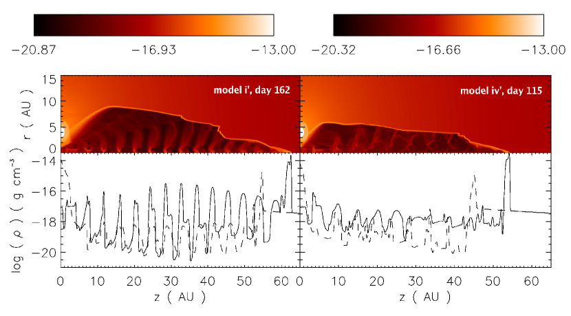
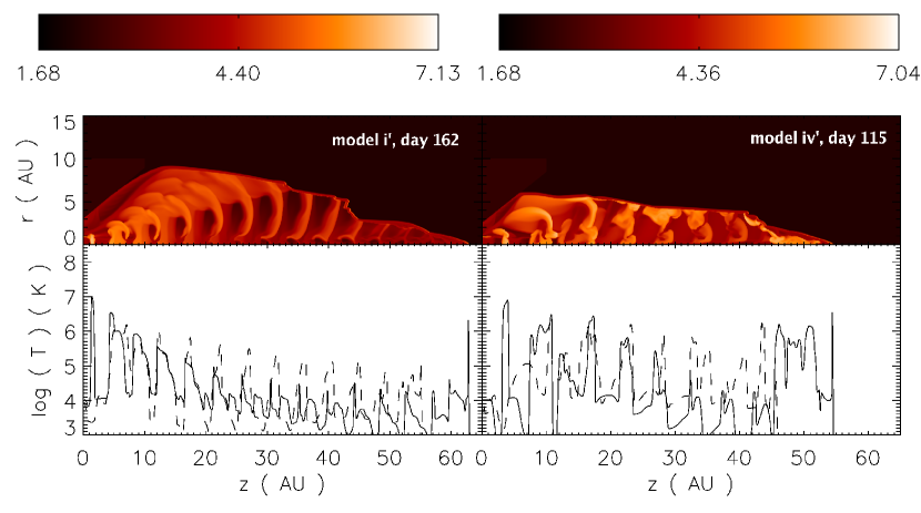
Figure 1.— Logarithm of density (top) and temperature (bottom) for model i’ on day 162 (left) and for model iv’ on day 115 (right), shown as contour plots and slices along the jet axis (solid) and parallel to the jet axis at $r=2$ AU (dashed).

Maps of logarithm of density and temperature for model i’ on day 162 and for model iv’ on day 115 are given in Fig. 1. Both are the last time-steps calculated.

2.2. Calculating the X-ray properties

We determined the expected X-ray flux using the density and temperature maps from the hydrodynamical simulations as follows. We used the atomic database ATOMDB with IDL including the Astrophysical Plasma Emission Database (APED) and the spectral models output from the Astrophysical Plasma Emission Code (APEC, Smith et al. 2001) to calculate the emissivity. The default abundances in ATOMDB, i.e. 14 elements (H, He, C, N, O, Ne, Mg, Al, Si, S, Ar, Ca, Fe, Ni) with solar abundances of Anders & Grevesse (1989), are used. The energy range is divided into bins of 0.01 keV. We compute the spectrum and the total flux in X-rays as a function of evolutionary time for each of our models.

We calculate the X-ray emission in the range between 0.15 – 15 keV, which is exactly the energy range covered by EPIC on XMM-Newton and includes that of the ACIS instrument (0.2 – 10 keV) and of HETG (0.4 – 10 keV) on Chandra. The emission from gas with a temperature lower than $\lesssim 10^{6}$ K is only marginal in this energy range.

3. The total X-ray luminosity and its time dependence

As expected, the high temperatures, created by the interaction of the jet pulses with previously ejected matter, lead to substantial X-ray emission (Fig. 2). The X-ray luminosity in model iv’ is higher than in model i’. This is a result of the higher density in the pulses and thus of the higher kinetic luminosity $L_{\rm jet}=1/2\,\dot{M}\,v^{2}$ pumped into the jet. Furthermore, in model i’ about 5% of the average kinetic luminosity is radiated in X-rays, but in model iv’ about 19%. Since the X-rays are emitted by shocked material from the fast moving pulses and since the X-ray luminosity is proportional to $\rho^{2}$, compared to $L_{\rm jet}$ being proportional to $\rho$, the ratio of the X-ray luminosity to the kinetic luminosity is proportional to $\rho$. Therefore this ratio is higher in model iv’ than in model i’.

Figure 2.— X-ray luminosity as a function of the evolution time of the jet in model i’ (solid) and model iv’ (dashed) in the energy range 0.15 – 15 keV. Most of the energy is emitted below 2 keV, i.e. the plots showing the luminosity in the energy range 0.15 – 2 keV are similar.

We find minima and maxima in the X-ray emission $L_{\rm X}$ (computed by integrating over the energy range 0.15 – 15 keV) which are connected with the periodic emergence of jet pulses (Fig. 3). Thus the period of the variations in the X-ray emission is about 7 days. The size of the fluctuations is 50 % and more of the average emission.

Figure 3.— X-ray luminosity as a function of time for model i’ (top) and model iv’ (bottom); one can see minima and maxima created by the emergence of each new jet pulse; the dotted lines in the top plots show the different trends of the X-ray luminosity decreases with time.

While the X-ray luminosity stays constant with time for model i’, it decreases with time for model iv’. This difference might be related to a larger amount of cooling in model iv’. The initial shock temperature is identical in both models, since the velocities are the same. The higher densities in the jet pulses in model iv’, however, lead to higher densities in the X-ray emitting material and thus to higher pressures which result in stronger adiabatic expansion and hence enhanced adiabatic cooling. Radiative cooling is also enhanced by the higher densities in model iv’.

4. The spectrum and its time dependence

The spectra of both models in the energy range between 0.15 – 15 keV show many different features. They show continuum emission, and superimposed on the continuum, a large number of emission features (some of which are blends of several emission lines). A prominent feature, which is mainly due to blended iron lines, is seen between 0.7–1 keV. Iron also produces a strong emission feature in the 6.4 – 6.7 keV range requiring very high temperatures ($\sim$ $10^{7}$ K) that are reached locally in the jet.

Figure 4.— Spectrum in the energy range between 0.15 – 15 keV; top: for model i’ on days 153 (a minimum of the total X-ray luminosity, solid) and 155 (close to the maximum X-ray luminosity, dashed), bottom: for model iv’ on days 105 (solid) and 107 (dashed). The spectrum plotted with a solid line is shifted downwards by a factor of 100 for clarity in each plot. One can clearly see the time dependence of the spectrum.

Like the total X-ray luminosity, the spectrum is also highly time-dependent (Fig. 4). We define two proxies for the temperature, one using the low energy spectrum and one using the high energy spectrum. These proxies can then be used conveniently for direct comparison with the single-temperature thermal plasma models typically used to fit the observed data.

4.1. Defining temperature proxies

In order to characterize the temperature of the propagating jet from the low energy spectrum, we use the fact that below energies of about 0.7 keV, both spectra in Fig. 4 are almost identical, but differ significantly between 0.7 and 2 keV. Therefore we define the proxy $\zeta$ for relatively low temperature plasma ($10^{7}$ K) in the jet as

$$\zeta=\frac{f_{\rm(0.2-0.7)\,keV}}{f_{\rm(0.7-2)\,keV}}$$ (2)

with $f_{\rm(0.2-0.7)\,keV}$ and $f_{\rm(0.7-2)\,keV}$ the fluxes integrated over the given energy ranges (Fig. 5, top).

The slope of the continuum also changes with time. To measure this behavior, we define a flux ratio

$$\xi=\frac{f_{\rm 4\,keV}}{f_{\rm 9\,keV}}$$ (3)

We choose regions in the spectrum where no lines are present, although photons with these high energies have not been observed from the jet or might be confused with photons from the central engine in observed spectra.

Figure 5.— Temperature proxies as a function of temperature for a single-temperature thermal plasma calculated with ATOMDB: hardness ratio $\zeta$ (top) and flux ratio $\xi$ (bottom) as defined in the text.

4.2. Determining the temperature from model spectra

In model i’, the high temperature proxy, $\log(\xi)$, varies with time spanning a range from 1.5 to 3. It has its highest value (i.e. the spectrum has the steepest slope, hence the average temperature is at its lowest value), when the X-ray luminosity shows a minimum (Fig. 6). Comparison of the model $\log(\xi)$ values with that of a single-temperature thermal plasma (Fig. 5, bottom) gives us temperature estimates of the hot component between $8\times 10^{6}$ K (0.69 keV) and $1.7\times 10^{7}$ K (1.5 keV). The highest temperatures are consistent with that of post-shock gas with a shock velocity of about 1100 km s^-1. The minimum in the $\log(\xi)$ (i.e. maximum in average temperature) coincides with the emergence of each new pulse; within the next 2–3 day period the compressed knot cools and the emissivity increases. Therefore the maximum in the X-ray luminosity is reached about 2–3 days later.

The low temperature proxy, $\log(\zeta)$, varies between about 0.5 and 1.6, the corresponding temperatures lie between $1.6\times 10^{6}$ K (0.14 keV) and $3\times 10^{6}$ K (0.26 keV). The jet is therefore better described as a combination of a warm and a hot component rather than as a single-temperature plasma.

Figure 6.— X-ray luminosity of the jet as a function of time in the energy range 0.15 – 15 keV (top), flux ratio $\xi$ as a function of time (middle) and hardness ratio $\zeta$ as a function of time (bottom) for models i’.

Figure 7.— same as Fig. 6, but for model iv’

In model iv’, $\log(\xi)$ varies between 2.1 and 2.8; the corresponding temperatures are $8\times 10^{6}$ K (0.69 keV) and $1.2\times 10^{7}$ K (1.03 keV). The low temperature proxy, $\log(\zeta)$, lies between 0.1 and 0.6; the corresponding temperatures are $3\times 10^{6}$ K (0.26 keV) and $3.8\times 10^{6}$ K (0.33 keV). As in model i’, the jet is better characterized as a combination of a warm and a hot component.

The range of temperatures in the hot component over one pulse cycle in model iv’ is smaller compared to that in model i’; this is because the higher density in model iv’ makes radiative cooling more efficient, such that the shock heating is damped more efficiently. The different density contrasts between the jet pulses and the steady jet in both models also lead to different shock velocities and thus to different shock temperatures to which the plasma is heated initially.

4.3. Emission lines in the model spectra

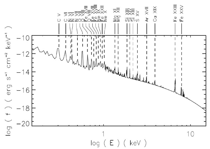
Figure 8.— Spectrum in the energy range between 0.15 – 15 keV for model i’ on days 155; several strong emission lines are present with very different ionization potentials which can only be explained using two components at different temperatures.

We have identified the strongest emission lines characterizing a typical jet spectrum using the spectrum derived from model i’ on day 155 as a template (Fig. 8). The most prominent lines are the oxygen line at 0.57 keV, the Ne lines at 0.93 and 1.03 keV, the Mg lines at 1.35 and 1.47 keV, the Si lines at 1.86, 2.01 and 2.18 keV, and the Fe complex at about 6.5 keV. All strong lines with their identifications are given in Table 2, including their fluxes at days 153 and 155 in model i’ and days 105 and 107 in model iv’. Most of these lines are hydrogenic or He-like lines of heavy elements, however, also lines of higher ionization states are present (Fe XXII, Fe XXIII, Fe XXV). Thus this set of lines with very different ionization potentials can also only explained with two components at different temperatures.

Table 2Prominent emission lines in the model spectra

ion	energy (keV)	flux (erg s-1 cm-2)
		model i’		model iv’
		day 153	day 155	day 105	day 107
C V	0.31	8.81$\times 10^{-14}$	7.02$\times 10^{-14}$	1.36$\times 10^{-13}$	7.03$\times 10^{-14}$
C VI	0.37	3.09$\times 10^{-14}$	2.49$\times 10^{-14}$	1.06$\times 10^{-13}$	4.21$\times 10^{-14}$
N VI	0.42	6.96$\times 10^{-15}$	6.53$\times 10^{-15}$	2.58$\times 10^{-14}$	1.08$\times 10^{-14}$
N VI	0.43	1.00$\times 10^{-14}$	9.20$\times 10^{-15}$	4.06$\times 10^{-14}$	1.50$\times 10^{-14}$
N VII	0.50	2.59$\times 10^{-15}$	3.07$\times 10^{-15}$	2.31$\times 10^{-14}$	1.68$\times 10^{-14}$
O VII	0.57	3.80$\times 10^{-14}$	3.67$\times 10^{-14}$	2.67$\times 10^{-13}$	1.59$\times 10^{-13}$
O VIII	0.65	5.57$\times 10^{-15}$	9.26$\times 10^{-15}$	1.11$\times 10^{-13}$	1.37$\times 10^{-13}$
Fe XVII	0.73	5.32$\times 10^{-16}$	3.70$\times 10^{-15}$	9.17$\times 10^{-14}$	8.93$\times 10^{-14}$
Fe XVII	0.83	5.73$\times 10^{-16}$	4.11$\times 10^{-15}$	9.34$\times 10^{-14}$	9.39$\times 10^{-14}$
O VIII	0.77	4.19$\times 10^{-16}$	1.65$\times 10^{-15}$	2.89$\times 10^{-14}$	3.13$\times 10^{-14}$
Fe XVIII	0.87	2.17$\times 10^{-17}$	7.42$\times 10^{-16}$	2.29$\times 10^{-14}$	2.68$\times 10^{-14}$
Ne IX	0.92	5.90$\times 10^{-16}$	1.99$\times 10^{-15}$	3.60$\times 10^{-14}$	5.00$\times 10^{-14}$
Fe XXII	0.97	1.30$\times 10^{-17}$	7.52$\times 10^{-16}$	1.41$\times 10^{-14}$	2.58$\times 10^{-14}$
Ne X	1.02	8.72$\times 10^{-17}$	1.70$\times 10^{-15}$	3.76$\times 10^{-14}$	4.17$\times 10^{-14}$
Mg XI	1.35	3.34$\times 10^{-17}$	4.00$\times 10^{-16}$	9.41$\times 10^{-15}$	1.07$\times 10^{-14}$
Mg XII	1.47	1.71$\times 10^{-18}$	2.72$\times 10^{-16}$	4.28$\times 10^{-15}$	7.17$\times 10^{-15}$
Si XIII	1.86	5.25$\times 10^{-18}$	3.86$\times 10^{-16}$	7.04$\times 10^{-15}$	1.06$\times 10^{-14}$
Si XIV	2.01	3.71$\times 10^{-19}$	2.12$\times 10^{-16}$	1.37$\times 10^{-15}$	4.30$\times 10^{-15}$
Si XIII	2.18	4.51$\times 10^{-19}$	3.81$\times 10^{-17}$	5.76$\times 10^{-16}$	9.99$\times 10^{-16}$
S XV	2.46	1.35$\times 10^{-18}$	1.43$\times 10^{-16}$	1.55$\times 10^{-15}$	3.34$\times 10^{-15}$
Ar XVII	3.14	6.06$\times 10^{-20}$	3.31$\times 10^{-17}$	2.03$\times 10^{-16}$	5.60$\times 10^{-16}$
Ca XIX	3.9	1.52$\times 10^{-20}$	1.05$\times 10^{-17}$	3.68$\times 10^{-17}$	1.30$\times 10^{-16}$
Fe XXIII	6.65	2.11$\times 10^{-20}$	4.01$\times 10^{-17}$	4.81$\times 10^{-18}$	2.01$\times 10^{-17}$
Fe XXV	7.78	1.17$\times 10^{-23}$	2.76$\times 10^{-18}$	1.17$\times 10^{-18}$	7.12$\times 10^{-18}$

5. The X-ray emission maps

The results in the previous section suggest the existence of two components, a warm one with temperatures in the range of (1.6 – 3.8)$\times 10^{6}$ K and a hot one with temperatures of (8 – 17)$\times 10^{6}$ K, respectively. As already pointed out in Paper I and II, the jet consists of dense, cool knots and tenuous, hot inter-knot gas. The knots are too cold to emit X-rays, thus the low and high energy components in the X-ray spectrum probe the temperature structure of the hot parts of the jet (Fig.1 and Fig. 12 in paper I). These hot parts consist of shocked material in the inter-knot gas segments. Temperature gradients are present within each inter-knot gas segment and also between the inter-knot gas close to the jet source and those downstream near the jet head. The regions with the highest temperatures and thus emission above 6 keV lie in the first two inter-knot gas segments within only a few AU from the central source (Fig. 9). The inter-knot gas segments become progressively cooler, as they move farther away from the jet source due to adiabatic expansion and the resulting cooling of jet material.

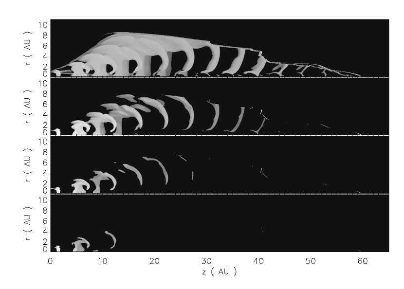
Figure 9.— Emission maps of model i’ on day 155 in the 0.15 – 1.5 keV range, in the 1.5 – 3 keV range, in the 3 – 6 keV range and in the 6 – 7 keV range.

6. Comparison with observations

We now compare the results of our models to X-ray observations of the three objects MWC 560 (only upper limits to the flux are available), CH Cyg and R Aqr.

6.1. MWC 560

The source fluxes in the 0.2 – 2.4 keV range are $3\times 10^{-13}$ erg s^-1 cm^-2 for model i’ and $2\times 10^{-12}$ erg s^-1 cm^-2 for model iv’, using a distance of 2.5 kpc to MWC 560 (Schmid et al. 2001, and references therein). The latter flux is reduced to an absorbed flux of $1.7\times 10^{-13}$ erg s^-1 cm^-2, using the model of the visual interstellar extinction in the Galaxy by Hakkila et al. (1997) which gives an $A_{\rm v}=0.88$ or $N_{\rm H}=1.55\times 10^{21}$ cm^-2 for MWC 560. The absorbed flux is consistent with MWC 560’s non-detection in the ROSAT all-sky survey ($<7\times 10^{-13}$ erg s^-1 cm^-2, Mürset et al. 1997). The fluxes, however, are high enough such that today’s X-ray telescope as Chandra and XMM-Newton should be able to detect MWC 560.

6.2. CH Cyg

Since the jet velocities are similar in MWC 560 and CH Cyg, we can make a detailed comparison of our models with the latter object. This comparison is limited to the soft emission from the propagating jet and excludes the X-ray emission above about 2 keV which is believed to be dominated by the variable scattered hard X-rays from the central source.

Ezuka et al. (1998) resolved for the first time atomic emission lines (or their blends) from elements in hydrogenic and He-like ionization states in the X-ray spectra of CH Cyg. The most prominent features in the observed spectra are the oxygen line at 0.57 keV, the blend of i) Ne lines at 0.93 and 1.03 keV, ii) Mg lines at 1.35 and 1.47 keV, iii) Si lines at 1.86, 2.01 and 2.18 keV, and the Fe line complex at about 6.5 keV. These lines are also seen in our model spectra. Furthermore, they also had to introduce a two-temperature thermal plasma model to explain the set of lines detected in the ASCA spectrum. The temperatures of their two components (0.21 and 0.72 keV) are in the same range as in our model i’ (warm component: 0.14 – 0.26 keV, hot component: 0.69 – 1.5 keV, see §4.2). In model iv’, the warm component is too hot (0.26 – 0.33 keV) to explain the observations.

Recently, KCR07 reported the detection of multiple components, including an arc, in the archival Chandra images. This arc has a similar opening angle to many of the arcs visible in our X-ray emission maps (Fig. 9), and its presence supports our pulsed-jet model in which such emission results from internal shocks generated by colliding jet ejecta.

Considering the smaller distance of 268 pc to CH Cyg, the model X-ray luminosity of $2.2\times 10^{32}$ erg s^-1 for model i’ and $1.5\times 10^{33}$ erg s^-1 for model iv’ in the 0.2 – 2 keV range implies fluxes of $2.6\times 10^{-11}$ erg s^-1 cm^-2 and $1.74\times 10^{-10}$ erg s^-1 cm^-2, respectively. The interstellar extinction for CH Cyg is $A_{\rm v}=0.006$ or $N_{\rm H}=1\times 10^{20}$ cm^-2, thus the absorbed flux is $2\times 10^{-11}$ erg s^-1 cm^-2 for model i’ and $1.3\times 10^{-10}$ erg s^-1 cm^-2 for model iv’, respectively. The measured fluxes of the soft components associated with the jet, however, lie in the range $(0.4-3.8)\times 10^{-12}$ erg s^-1 cm^-2 (Ezuka et al. 1998; Galloway & Sokoloski 2004; Mukai et al. 2006). Since these measured fluxes are smaller than those predicted by model i’ and by far smaller than those from model iv’ which has a higher jet pulse density than model i’, we infer that the jet pulse densities in CH Cyg are smaller than those in MWC 560 and our models. If, as stated in §3, the ratio of the X-ray luminosity to the kinetic energy pumped into the jet is proportional to the jet pulse density, we can estimate that the jet pulse density has to be reduced to about $10^{5}$ cm^-3 to model the X-ray flux observed in CH Cyg. In order to resolve the difference between measured and model fluxes with uncertainties in the distance to CH Cyg, the latter would have to be about 700 pc, however, this large value is very unlikely, since the distance was measured with HIPPARCOS with an error of 23 %.

KCR07 give an observational estimate of the density in the jet, 50 cm^-3, based on the total X-ray luminosity, assuming an emitting sphere with a radius of 400 AU and a mean emissivity of $2\times 10^{-23}$ erg cm³ s^-1. However, astrophysical jets, typically, are collimated structures which have significantly smaller volumes than a sphere. Since we simulated the propagation of the model jets only up to a length of 65 AU, not 400 AU, we scale up its volume as follows. If we assume that the cross-sectional area stays constant as the jet propagates and evolves with time, the jet volume is about ($\pi\,\times 6^{2}\times 400$) AU³ (Fig. 9) which is smaller by about a factor of 6000 than that of a sphere with a radius of 400 AU. Alternately if we assume that the lateral expansion of the jet is proportional to its axial expansion, the volume is still overestimated by a factor of about 160. Furthermore, within the volume of the jet, the X-rays are emitted by clumps and not by the whole jet, i.e. the filling factor for the X-ray emission is, $f_{1}<1$. In addition, KCR07 assume a temperature of $1.2\times 10^{7}$ K (1 keV) to estimate the emissivity, however, our jet models show that such high temperatures are only archieved in the innermost region of the jet; at larger distances from the jet source along the axis, the X-ray emitting knots are significantly cooler (Fig. 1). Thus the value of the emissitivity should be lower and the density should be higher than estimated by KCR07 by another correction factor $f_{2}>1$. Hence we conclude that an accurate estimate of the X-ray emitting volume and the temperature would lead to a higher density by a factor of (160–6000)$f_{2}/f_{1}$ compared to the value given by KCR07, of the order of $10^{4}$–$10^{6}$ cm^-3. This range compares well with the densities of material emitting soft X-rays in our models which are of the order of $10^{5}$–$10^{6}$ cm^-3 (Fig. 1).

Other possibilities to reduce the X-ray fluxes in our models, bringing them closer to the observed ones in CH Cyg, are i) a longer timescale between the pulses and ii) a smaller velocity difference between the steady jet and the jet pulses. In the first case, less energy is pumped into the jet and each jet knot and the jet head can cool further before being hit by the next pulse. In the second case, the smaller velocity difference reduces the temperature to which the shocked material is heated. However, the density contrast then also has to be adjusted in order to reproduce the observed proper motion of the jet knots. Which of the above scenarios is the most likely one can only be determined from future simulations which have been fine-tuned to fit the properties of the X-ray emitting material in the jet of CH Cyg.

In 1994 and 2006, the flux from the jet in CH Cyg was almost at the same level, in the range $(2.7-3.8)\times 10^{-12}$ erg s^-1 cm^-2 (Ezuka et al. 1998; Mukai et al. 2006). In 2001, however, it was lower by a factor of ten (Galloway & Sokoloski 2004). In the context of our models, such a drop in flux may result from a large decrease in the density of the pulses which may be caused by a drop in the accretion rate onto the white dwarf.

6.3. R Aqr

Since the jet velocity in R Aqr is smaller by a factor of 2 than those in our models, we can only make a more limited comparison of the model results with the observations. Kellogg et al. (2006) and also Korreck et al. (2006) report a tangential motion of an X-ray emitting knot of 600 km s^-1. Korreck et al. (2006) estimated a density of 100 cm^-3, however, it may be possible that, as in the case of CH Cyg, the X-ray emitting volume is overestimated and thus the density is underestimated.

Kellogg et al. (2001) found in R Aqr that the NE jet is more luminous by a factor of 3 than the SW jet. The spectrum the NE jet was fitted with a single-temperature thermal plasma with a temperature of 1.66 keV, the spectrum of the SW jet with a plasma temperature of 0.2 keV. The simplest explanation of this difference is that the ambient media on both sides have different densities which would lead to different compression factors and thus to different shock heating temperatures. However, proper motion measurements show no significant differences in the velocities of the knots in both sides of the jet (Paresce & Hack 1994; Mäkinen et al. 2004), which we would expect if different ambient densities would decelerate the jet differently on both sides.

Our modeling can provide a plausible explanation for the observed differences between the two sides of the jet, if we assume that the ejection of the jet pulses on both sides are out of phase with each other. Hollis et al. (1991) derived a kinematic age of both jets of about 90 yrs; over the extent of the jet we can observe 3–6 knots in the observations of e.g. Paresce & Hack (1994) which suggests several ejection events in this period of time. A period of about 17 years for these ejection events has been inferred from radio observations (Kafatos et al. 1989), thus they are significantly larger than in MWC 560 and in our models. We hypothesize that the X-ray emitting blobs in the NE jet were ejected later than those in the SW jet and therefore have cooled less. This hypothesis is supported by the fact that the X-ray emitting component in the NE jet is closer to the central core (about 8”) than the blobs in the SW jet (12–26”, Kellogg et al. 2001). A new SW jet component with an offset of about 1.5” from the central source has recently been reported by Nichols et al. (2007). Assuming a jet velocity of about 600 km s^-1 (Kellogg et al. 2006), i.e. about 0.6” per year, we obtain a kinematic age of about 2.5 years for this component. Even if the new component had been ejected during the epoch of Kellogg et al. (2001)’s observations, its flux would have contributed to the central source, but not to that of the SW jet. Hence the presence of the new component does not conflict with our hypothesis. The time period between the emergence of the new SW jet component and the emergence of the blob now located at 12” is about 17 years which supports the inferred period for the ejection of jet pulses in R Aqr.

In §3, we showed that the total X-ray luminosity decreases with time, probably due to adiabatic cooling in the jet (Paper II). This effect provides a plausible explanation of the decrease in X-ray flux in the jet of R Aqr from a value of $5\times 10^{-13}$ erg s^-1 cm^-2 in the early 1990s (Hünsch et al. 1998) to $1\times 10^{-13}$ erg s^-1 cm^-2 in 2000 (Kellogg et al. 2001). If this explanation holds, we expect to see a further decrease in flux in future observations.

6.4. The 6.4 – 6.7 keV iron line complex

This iron line complex has been observed in both objects, CH Cyg and R Aqr. Our model spectra also show the existence of this Fe line complex (§4). Ezuka et al. (1998) fitted the observed spectrum of CH Cyg with three single-temperature components (a warm and a hot component to explain the jet emission and hard component for the central engine) and an additional Gaussian representing fluorescence emission in the Fe K$\alpha$ line. This fluorescence occurs close to the white dwarf and the accretion disk. Since it is not possible to disentangle the flux of the thermal and the fluorescence components in this line complex and since our models do not include the effect of fluorescence, we cannot compare our models with this part of the observed spectrum of CH Cyg.

In R Aqr, the origin of the hard X-ray emission is more ambiguous. Kellogg et al. (2001) detected 16 photons in the range between 6.4 and 6.7 keV which they attribute to the central source due to the extraction regions they chose. The physical origin of this emission, i.e. thermal or fluorescence, cannot be decided, since there are not enough photons to model the spectrum in this energy and characterize its nature. In our model, we find significant hard radiation including continuum and iron emission lines, being emitted by the first two internal shocks in the jet downstream from the source (i.e. at a distance less than 15 AU). Since at R Aqr’s distance of 200 pc, 15 AU correspond to 75 milliarcseconds, which is well below the angular resolution of Chandra, the X-ray emission from these shocks cannot be separated from the central source. The model X-ray luminosity in the 6.4–6.7 keV range is between $5.1\times 10^{24}$ erg s^-1 and $7.3\times 10^{28}$ erg s^-1 for model i’ and between $2.8\times 10^{28}$ erg s^-1 and $5.1\times 10^{29}$ erg s^-1 for model iv’, respectively, depending on whether the jet is in its minimum or maximum state. At a distance of 200 pc, this corresponds to fluxes between $1.1\times 10^{-18}$ erg s^-1 cm^-2 and $1.1\times 10^{-13}$ erg s^-1 cm^-2. Since Kellogg et al. (2001) measured a flux of $4.9\times 10^{-14}$ erg s^-1 cm^-2 at 6.41 keV, we suggest that the measured iron line flux may be emitted by the jet itself, and an additional fluorescence component is not needed, in R Aqr. However, new simulations with the same jet velocity as in R Aqr are needed in order to test this suggestion.

7. Conclusions

We have used our models of pulsed, radiative jets in symbiotic stars in order to investigate their X-ray properties in detail. These models show that the well-studied pole-on jet in MWC 560 should be easily detected by today’s X-ray telescopes such as Chandra and XMM-Newton, since our model flux and its time variation for this source are of the order of $10^{-13}$ erg s^-1 cm^-2.

We find minima and maxima in the X-ray emission $L_{\rm X}$ (computed by integrating over the energy range 0.15 – 15 keV) which are connected with the periodic emergence of jet pulses. The maxima of the total X-ray luminosity occur 2–3 days after the emergence of new jet pulses, which are ejected every 7 days. The size of the fluctuations is 50 % and more of the average emission, making such X-ray flashing jets detectable with Chandra and XMM-Newton.

The X-ray spectra of our model jets are rich in emission line features, the most prominent of which correspond to observed features in the spectra of CH Cyg.

By using low and high energy temperature proxies derived from the spectra, we can show that the emission can be adequately characterized with a hot and a warm optically-thin plasma component. The hot component has temperature values of about 0.7 keV (1.6 keV) during the minima (maxima) of the total X-ray luminosity and the warm component has temperature values of about 0.14 keV (0.33 keV) during the minima (maxima).

While model iv’ is appropriate for MWC 560, we have shown that model i’, which has a lower jet pulse density than model iv’, is more appropriate for the jet in CH Cyg in terms of explaining the lower X-ray flux. Other possibilities to reduce the flux are a longer timescale between the pulses and a smaller velocity difference between the steady jet and the jet pulses. Which of the above scenarios is the most likely one has to be tested in future simulations which have to be tuned to the jet in CH Cyg.

Our models also offer a plausible explanation for the differences in luminosities and temperatures in the NE and the SW jet of R Aqr. We assume that the ejection of the jet pulses on both sides are out of phase with each other. We hypothesize that the X-ray emitting blobs in the NE jet were ejected later than those in the SW jet and therefore have cooled less.

We find the existence of iron line emission in the 6.4 – 6.7 keV range in our models which is also observed in both, CH Cyg and R Aqr. Our models cannot be directly applied to CH Cyg, because of an additional fluorescence component from the central source and accretion disk in the observed spectrum and because fluorescence is not included in our models. In the case of R Aqr, although this emission has been associated with the central source, our modeling shows that it is consistent with being produced by jet knots very close to the latter, because their separation in our model is well below the angular resolution of Chandra.

Using our current models which were built to fit the optical data of the jet in MWC 560 we are able to explain some of the important characteristics of X-ray emission from jets in MWC 560 and other symbiotic stars. The results of this study demonstrate the great potential of future numerical simulations of pulsed jets which have been fine-tuned to specific source properties for understanding the jet phenomenon in symbiotic stars. Furthermore, we hope that this study will inspire new and more sensitive observations of X-ray emission from jets in symbiotic stars.

References

- Anders & Grevesse (1989) Anders, E., Grevesse, N. 1989, GeCoA 53, 197
- Anderson et al. (2003) Anderson, J. M., Li, Z.-Y., Krasnopolsky, R., Blandford, R. D. 2003, ApJ 590, L107
- Blandford & Payne (1982) Blandford, R. D., Payne, D. G. 1982, MNRAS 199, 883
- Ezuka et al. (1998) Ezuka, H., Ishida, M., Makino, F. 1998, ApJ 499, 388
- Eyres et al. (2002) Eyres, S. P. S., Bode, M. F., Skopal, A., et al. 2002, MNRAS 335, 526l
- Galloway & Sokoloski (2004) Galloway, D. K., Sokoloski, J. L. 2004, ApJ 613, L61
- Goodson et al. (1997) Goodson, A. P., Winglee, R. M., Böhm, K.-H. 1997, ApJ 489,199
- Hakkila et al. (1997) Hakkila, J., Myers, J. M., Stidham, B. J., Hartmann, D. H. 1997, AJ 114, 2043
- Hollis et al. (1985a) Hollis, J.M., Michalitsianos, A. G., Kafatos, M., et al. 1985, ApJ 289, 765
- Hollis et al. (1985b) Hollis, J. M., Lyon, R. G., Dorband, J. E., et al. 1985, ApJ 475, 231
- Hollis et al. (1991) Hollis, J. M., Oliversen, R. J., Michalitsianos, A. G., et al. 1991, ApJ 377, 227
- Hollis et al. (1997) Hollis, J. M., Pedelty, J. A., Lyon, R. G. 1997, ApJ 482, L85
- Hünsch et al. (1998) Hünsch, M., Schmitt, J. H., Schroeder, K., Zickgraf, F. 1998, A&A 330, 225
- Kafatos et al. (1989) Kafatos, M., Hollis, J. M., Yusef-Zadeh, F., et al. 1989, ApJ 346, 991
- Karovska et al. (2007) Karovska, M., Carilli, C. L., Raymond, J. C., Mattei, J. A. 2007, ApJ accepted, astro-ph/0703278
- Kellogg et al. (2001) Kellogg, E., Pedelty, J. A., Lyon, R. G. 2001, ApJ 563, 151
- Kellogg et al. (2006) Kellogg, E., Anderson, C., DePasquale, J., et al. 2006, poster abstract #70.08, American Astronomical Society Meeting 207
- Korreck et al. (2006) Korreck, K. E., Kellogg, E., Sokoloski, J. L. 2006, in: ”The Multicoloured Landscape of Compact Objects and their Explosive Origins”, astro-ph/0611401
- Leahy & Taylor (1987) Leahy, D. A., Taylor, A. R. 1987, A&A 176, 262
- Mäkinen et al. (2004) Mäkinen, K., Lehto, H. J., Vainio, R., Johnson, D. R. H. 2004, A&A 424, 157
- Matt et al. (2002) Matt, S., Goodson, A. P., Winglee, R. M., Böhm, K.-H. 2002, ApJ 574, 232
- Mukai et al. (2006) Mukai, K., Ishida, M., Kilbourne, C., et al. 2006, PASJ accepted, astro-ph/0609245
- Mürset et al. (1997) Mürset, U., Wolff, B., Jordan, S. 1997 , A&A 319, 201
- Nichols et al. (2007) Nichols, J. S., DePasquale, J., Kellogg, E., et al. 2007, ApJ accepted
- Paresce & Hack (1994) Paresce, F., Hack, W. 1994, A&A 287, 154
- Schmid et al. (2001) Schmid, H. M., Kaufer, A., Camenzind, M., et al. 2001, A&A 377, 206
- Smith et al. (2001) Smith, R. K., Brickhouse, N. S., Liedahl, D. A., Raymond, J. C. 2001, ApJ 556, L91
- Solf & Ulrich (1985) Solf, J., Ulrich, H. 1985, A&A 148, 274
- Stute (2006) Stute, M., 2006, A&A 450, 645 (Paper II)
- Stute, Camenzind & Schmid (2005) Stute, M., Camenzind, M., Schmid, H. M. 2005, A&A 429, 209 (Paper I)
- Sutherland & Dopita (1993) Sutherland, R. S., Dopita, M. A. 1993, ApJS, 88, 253
- Taylor et al. (1986) Taylor, A. R., Seaquist, E. R., Mattei, J. A. 1986, Nature, 319, 38
- Thiele (2000) Thiele, M. 2000, Numerical simulations of protostellar jets, PhD Thesis, University of Heidelberg
- Viotti et al. (1987) Viotti, R., Piro, L., Friedjung, M., Cassatella, A. 1987, ApJ 319, L7
- Wheatley & Kallman (2006) Wheatley, P. J., Kallman, T. R. 2006, MNRAS 372, 1602
- Ziegler & Yorke (1997) Ziegler, U., Yorke, H. 1997, Comp. Phys. Comm. 101, 54