Stability in random Boolean cellular automata on the integer lattice

F. Michel Dekking, Leonard van Driel and Anne Fey Delft Institute of Applied Mathematics, Technical University of Delft, Mekelweg 4, 2628 CD Delft, The Netherlands
email: F.M.Dekking@tudelft.nl
Eurandom, Eindhoven, The Netherlands
email: Fey@eurandom.tue.nl
Abstract.

We consider one-dimensional random boolean cellular automata, i.e., the cells are identified with the integers from 1 to $N$. The behavior of the automaton is mainly determined by the support of the random variable that selects one of the sixteen possible Boolean rules, independently for each cell. A cell is said to stabilize if it will not change its state anymore after some time. We classify the one-dimensional random boolean automata according to the positivity of their probability of stabilization. Here is an example of a consequence of our results: if the support contains at least 5 rules, then asymptotically as $N\rightarrow\infty$ the probability of stabilization is positive, whereas there exist random boolean cellular automata with 4 rules in their support for which this probability tends to 0.

1. Introduction

We study the dynamics of cellular automata as amply discussed in Stephen Wolfram’s book “A New Kind of Science” ([12]). The cells, which are identified with the integers from 1 to $N$, can be in two possible states 0 or 1, and the state at the next time instant is a function of the states of the two neighbouring cells. For this function, also called (evolution) rule, there are 16 different possibilities, see also Table 1. Although there is a chapter in [12] on random initial conditions for CA’s, there is hardly anything on random rules, or even on the possibility to assign different rules to different cells (so called inhomogeneous CA’s). In this paper we will give a classification of one-dimensional Random Boolean CA’s.

Our results are also of interest in the context of Random Boolean Networks introduced by Stuart Kauffman in 1969 ([3]). Here not only the rules and the initial condition are chosen randomly, but also the neighbours of a cell, i.e., the $N$ cells obtain a random graph structure. For each cell $i$ independently a mother $M(i)$ and a father $F(i)$ are chosen uniformly from the remaining pairs of cells. This gives a graph with vertices $i$ and directed edges $(M(i),i)$, $(F(i),i)$ for $i=1,\dots,N$. Next, each cell $i$ is assigned independently a Boolean rule $\Phi_{i}$ uniformly from the set of 16 Boolean rules (i.e., maps from $\{0,1\}^{2}$ to $\{0,1\}$, see also Table 1). To start, all cells obtain independently an initial value $X_{i}(0)$ from the set $\{0,1\}$ with equal probability. The state of a RBN at time $t$ will be denoted by $X(t)$. Then the dynamics is given by the map $\Psi_{\!\Phi}$:

$$X(t+1)=\Psi_{\!\Phi}(X(t))$$

defined by

$$X_{i}(t+1)=\Phi_{i}(X_{M(i)}(t),X_{F(i)}(t))$$

for all cells $i$.

A $1$-dimensional random Boolean cellular automaton can be considered as an RBN with
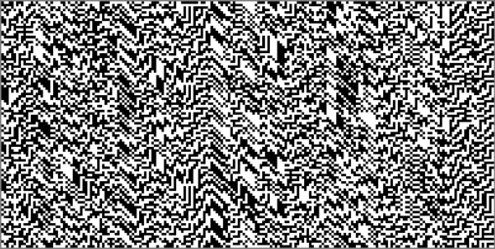
$$M(i)\equiv i-1\quad\mathrm{and}\quad F(i)\equiv i+1,$$

for $i\!=\!2,\dots,N\!-\!1$. We put $M(1)\!=\!N,F(1)\!=\!2$, and $M(N)\!=\!N-1,F(N)\!=\!1$. In Figure 1 we display a realization of the evolution of a RBCA in the usual way: zero’s and ones are coded by white and black squares, space is in the horizontal direction, time in the vertical direction.

Refer to caption
Figure 1. Evolution of a one-dimensional RBCA. After two time steps, most cells already become periodic. After five steps, the whole CA is periodic.

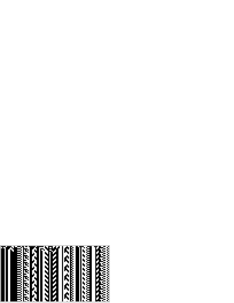
We say a cell stabilizes if its value is not changed anymore after some time. In Figure 1 the stable cells yield the black or white stripes; in this RBCA example about 56% of the cells stabilize.

Kauffman ([4]) found in his simulations that about 60-80% of the cells in a two-connected RBN stabilize. It was later shown rigorously by Luczak and Cohen ([5]) that in the limit as the number of cells $N$ tends to infinity 100% of the cells will stabilize—size $N=10\,000$ in Kauffmans simulations is much too small to unearth this behavior.
For the RBN’s there is no natural model for the infinite size ($N\rightarrow\infty$) network. For a one-dimensional CA there is: the graph is simply the set of all integers with edges between nearest neighbors. It therefore makes sense to speak of the probability $\sigma_{*}$ of stabilization of the infinite automaton. The result of Luczak and Cohen leads to the question whether this $\sigma_{*}=1$. In this paper we will show that this is rarely the case, and moreover that there are many cases where actually $\sigma_{*}=0$. By different cases we mean different distributions on the set of 16 Boolean rules. We remark that the results in [4] and [5] are restricted to the uniform distribution on the set of rules—see [2, 6, 7, 8] for some results for RBN’s with other rule distributions.
The second problem we will discuss is whether $\sigma_{N}\rightarrow\sigma_{*}$ when $N\rightarrow\infty$. We will show that this will often be the case, but may also fail to hold.
For some previous work with rather partial results on 2–dimensional versions of RBCA’s see e.g., [1]. We will give an application of our results at the end of Section 4 to a recent paper on RBN’s of Greil and Drossel ([2]).

Finally we mention that our interest in RBCA was also motivated by certain CA models of the subsurface in the geosciences (see  [11]).

2. Random Boolean cellular automata

Before we define RBCA, we describe their realizations which are inhomogeneous cellular automata. The dynamics in such a CA is defined by attaching a Boolean rule to each cell. The rule is given by specifying what its value is on the four different values $(1,1)$, $(1,0)$, $(0,1)$ and $(0,0)$ of the neighbors of a cell. In Table 1, all 16 different rules are defined.

Table 1. Definition of the 16 Boolean rules. The last column gives a formula for $\varphi_{\mathtt{j}}(x,y)$ when $\varphi_{\mathtt{j}}$ is affine.
$\mathtt{j}$ $\!\varphi_{\mathtt{j}}(0,0)\!$ $\varphi_{\mathtt{j}}(0,1)$ $\varphi_{\mathtt{j}}(1,0)$ $\varphi_{\mathtt{j}}(1,1)$ affine$I^{I^{2}}_{I_{2}}$
0 0 0 0 0 00
1 1 0 0 0 no
2 0 1 0 0 no
3 1 1 0 0 $x+1$
4 0 0 1 0 no
5 1 0 1 0 $y+1$
6 0 1 1 0 $x+y$
7 1 1 1 0 no
8 0 0 0 1 no
9 1 0 0 1 $x+y+1$
10 0 1 0 1 $y$
11 1 1 0 1 no
12 0 0 1 1 $x$
13 1 0 1 1 no
14 0 1 1 1 no
15 1 1 1 1 $1$

For ease of notation these are indexed as $\varphi_{\mathtt{j}}$ where $\mathtt{j}$ is the number in binary notation obtained from the four bits in the row describing $\varphi_{\mathtt{j}}$. Anytime we refer to one of these 16 rules we use index $\mathtt{j}$ (note the different font); when we use index $i$ we refer abusively to the rule assigned to cell $i$.

An inhomogeneous CA’s mapping $\Psi_{\varphi}:\{0,1\}^{N}\to\{0,1\}^{N}$ is determined by a vector of rules, $\varphi=(\varphi_{1},\ldots,\varphi_{N})$. Here for all time steps, $\varphi_{i}$ is the rule of cell $i$. Hence given a state $x=(x_{1}\ldots x_{N})$ we get $(\Psi_{\varphi}(x))_{i}=\varphi_{i}(x_{i-1},x_{i+1})$ for $i=2,\dots,N-1$. To deal with the problem that occurs in the end points we consider the automata as defined on a circle; a convenient way to express this is to define $x_{i+kN}=x_{i}$ for $i=1,\dots,N$, and all integers $k$.

To address $\Psi_{\varphi}$ we will also write the vector of lower indices of the $\varphi_{i}$ $(1\leq i\leq N)$ mentioned. E.g., mapping (0,3,3,15) describes $\Psi_{\varphi}:\{0,1\}^{4}\to\{0,1\}^{4}$ with rule vector $(\varphi_{\mathtt{0}},\varphi_{\mathtt{3}},\varphi_{\mathtt{3}},\varphi_{\mathtt{15}})$.

In a RBCA the rules $\varphi_{i}$ are chosen according to a distribution $\Phi$ on the set of rules, independently for each $i$. The initial state is an i.i.d. sequence $(X_{i}(0))$ from a Bernoulli(1/2) distribution, independent from the $(\Phi_{i})$. Then the value of the $i^{\textrm{th}}$ cell at time $t+1$ is given by

(1) $$X_{i}(t+1)=\Phi_{i}(X_{i-1}(t),X_{i+1}(t)).$$

We denote by ${{\mathbb{P}\!}_{N}}$ the probability measure generated by the ($X_{i}(0)$) and the ($\Phi_{i}$) on the space of infinite periodic sequences with period $N$. It is natural to consider also the probability measure ${{\mathbb{P}\!}_{*}}$ on $\{0,1\}^{\mathbb{Z}}$ generated by two infinite independent i.i.d. sequences ($X_{i}(0)$) and ($\Phi_{i}$).

3. Stability

We say cell $i$ stabilizes at time $T$ if

$$X_{i}(t)=X_{i}(T)\quad\text{for all }t\geq T,$$

and $T$ is the smallest integer with this property. Let $\sigma_{N}$ be the probability that a cell in a random cellular automaton of size $N$ with rule distribution $\Phi$ stabilizes. Because of stationarity,

$$\sigma_{N}={\mathbb{P}\!}_{N}\!\left({\text{cell }0\text{ stabilizes}}\right).$$

We first give an example were $\sigma_{N}$ does not converge as $N\rightarrow\infty$.
Consider the RBCA’s for $N=1,2\dots$ with rule distribution given by

$${\mathbb{P}\!}_{N}\!\left({\Phi=\varphi_{\mathtt{6}}}\right)=1.$$

Note that randomness is only involved because of the randomness in the initial state $X(0)=(X_{i}(0))$, and that $\varphi_{\mathtt{6}}$ is the well known linear rule which can be written as $\varphi_{\mathtt{6}}(x,y)=x+y$. This addition, as all additions with 0’s and 1’s, is modulo 2.

Proposition 1.

For the $\varphi_{\mathtt{6}}$-RBCA one has

$$\liminf_{N\rightarrow\infty}\sigma_{N}=0,\qquad\limsup_{N\rightarrow\infty}\sigma_{N}=1.$$

Proof: It is well known (see e.g. [10]) and easy to prove that the $\varphi_{\mathtt{6}}$-automaton satisfies

$$X_{i}(t)=X_{i-t}(0)+X_{i+t}(0)\qquad\text{ if }t=2^{p}\text{ for some }p.$$

It follows that $\sigma_{N}=1$ for each $N=2^{p}$ which is a power of 2:

$$X_{i}(N)=X_{-N+i}(0)+X_{N+i}(0)=2X_{i}(0)=0\qquad\text{for all }i,$$

which implies that $X_{i}(t)=0$ for all $t\geq N$. This proves that $\limsup\sigma_{N}=1$. To obtain the statement on $\liminf$, consider the subsequence of $N$ of the form $N=2^{p}+1$. Then we find for all $i$

$$X_{i}(N-1)=X_{i}(2^{p})=X_{-2^{p}+i}(0)+X_{2^{p}+i}(0)=X_{i+1}(0)+X_{i-1}(0).$$

From this we directly obtain that

$$X_{0}(N)=X_{-1}(N-1)+X_{1}(N-1)=X_{-2}(0)+X_{0}(0)+X_{0}(0)+X_{2}(0),$$

and so

(2) $$X_{0}(N)=X_{-2}(0)+X_{2}(0).$$

Thus

$${\mathbb{P}\!}_{N}\!\left({X_{0}(N-1)\neq X_{0}(N)}\right)={\mathbb{P}\!}_{N}\!\left({X_{-1}(0)+X_{1}(0)\neq X_{-2}(0)+X_{2}(0)}\right)=\frac{1}{2}.$$

Note that this computation does not only hold for $t=N-1$, but for any $t$ which satisfies $t=-1\mod N$. An infinite sequence of such $t$’s is given by $t=2^{(2k+1)p},k=0,1,2,\dots$. For $N$ of the form $2^{p}+1$ we therefore obtain that

$$1-\sigma_{N}={\mathbb{P}\!}_{N}\!\left({X_{0}(t)\neq X_{0}(t+1)\quad\text{for infinitely many }t}\right)\geq\frac{1}{2}.$$

This inequality is a warm up for a more general result: we can generalize Equation (2) to for all $m$

$$X_{0}(N+2^{m}-2)=X_{-2^{m}}(0)+X_{2^{m}}(0).$$

Since for $m=0,1,\dots,\ell$ the $X_{-2^{m}}(0)+X_{2^{m}}(0)$ are independent Bernoulli variables with success probability $1/2$, it follows that

$${\mathbb{P}\!}_{N}\!\left({\exists m,0\leq m<\ell:X_{0}(N+2^{m}-2)\neq X_{0}(N-1)}\right)=1-\frac{1}{2^{\ell}},$$

and employing the same infinite sequence of $t$’s as for the $\ell=1$ case, we can deduce that $\liminf_{N\rightarrow\infty}\sigma_{N}=0$. $\Box$

It is convenient to define random variables $Z_{i}$ by $Z_{i}=1$ if cell $i$ stabilizes, and 0 otherwise. We then have (independently of $i$):

$$\sigma_{N}={\mathbb{P}\!}_{N}\!\left({Z_{i}=1}\right),\quad\text{and}\quad\sigma_{*}={\mathbb{P}\!}_{*}\!\left({Z_{i}=1}\right).$$

The uniform RBCA is given by the rule distribution ${\mathbb{P}\!}_{N}\!\left({\Phi=\varphi_{\mathtt{j}}}\right)=1/16$ for $j=0,1,\ldots,15$.

Proposition 2.

Let $\sigma_{N}$ be the probability of stabilization of a size $N$ uniform RBCA, $\sigma_{*}$ that of an infinite size uniform RBCA. Then

$$\lim_{N\rightarrow\infty}\sigma_{N}=\sigma_{*}\quad\textrm{and}\quad\sigma_{*}>0.$$

Proof: The two rules $\varphi_{\mathtt{0}}$ and $\varphi_{\mathtt{15}}$ are called walls. We denote $W=\{\varphi_{\mathtt{0}}$,$\varphi_{\mathtt{15}}\}$. Cells that have obtained a rule from $W$ are already stable at time 0 or 1. We define for positive integers $k$ and $l$ the chambers $C_{k,l}$ by

$$C_{k,l}=\{\Phi_{-k}\in W,\Phi_{-k+1}\notin W,\Phi_{-k+2}\notin W,\ldots,\Phi_{\l-1}\notin W,\Phi_{l}\in W\}.$$

In addition we put $C_{0,0}=\{\Phi_{0}\in W\}$. Since the chambers are disjoint events whose union has probability 1 we can write

$\displaystyle\sigma_{*}={\mathbb{P}\!}_{*}\!\left({Z_{0}=1}\right)={\mathbb{P}\!}_{*}\!\left(Z_{0}=1\,|\,C_{0,0}\right){\mathbb{P}\!}_{*}\!\left({C_{0,0}}\right)+\sum_{k,l=1}^{\infty}{\mathbb{P}\!}_{*}\!\left(Z_{0}=1\,|\,C_{k,l}\right){\mathbb{P}\!}_{*}\!\left({C_{k,l}}\right).$

We will make a similar splitting for finite RBCA of size $N$. In case $N=2M+1$ we consider the indices of the chambers from the set $\{-M,\dots,0,\dots,M\}$, in case $N=2M$ from $\{-M\!+\!1,\dots,0,\dots,M\}$. In the sequel we will assume $N$ is odd, as our arguments can be transferred trivially to the case $N$ even. Let $D$ be the event

$$D=\Big{(}C_{0,0}\cup\bigcup_{k,l=1}^{M}C_{k,l}\Big{)}^{c}.$$

Then $D$ occurs iff there is no wall among $\Phi_{-M},\dots,\Phi_{0}$ or among $\Phi_{0},\dots,\Phi_{M}$. Since ${\mathbb{P}\!}_{N}\!\left({\Phi_{i}\notin W}\right)={\mathbb{P}\!}_{*}\!\left({\Phi_{i}\notin W}\right)=7/8$, we obtain that

$${\mathbb{P}\!}_{*}\!\left({D}\right)={\mathbb{P}\!}_{N}\!\left({D}\right)=2\Big{(}\frac{7}{8}\Big{)}^{M+1}\!\!-\Big{(}\frac{7}{8}\Big{)}^{2M+1}\leq 2\Big{(}\frac{7}{8}\Big{)}^{N/2}.$$

The crux of the proof is that for all $1\leq k,l\leq M$ and for $k=l=0$ we have

$${\mathbb{P}\!}_{N}\!\left(Z_{0}=1\,|\,C_{k,l}\right)={\mathbb{P}\!}_{*}\!\left(Z_{0}=1\,|\,C_{k,l}\right),$$

simply because both the finite automaton and the infinite automaton evolve between the walls independently of the evolution outside the walls. Thus

$\displaystyle|\sigma_{N}-\sigma_{*}|$ $\displaystyle\leq$ $\displaystyle{\mathbb{P}\!}_{*}\!\left(Z_{0}=1\,|\,D\right){\mathbb{P}\!}_{*}\!\left({D}\right)+{\mathbb{P}\!}_{N}\!\left(Z_{0}=1\,|\,D\right){\mathbb{P}\!}_{N}\!\left({D}\right)$
$\displaystyle\leq$ $\displaystyle 4\Big{(}\frac{7}{8}\Big{)}^{N/2}.$

It follows that $\sigma_{N}\rightarrow\sigma_{*}$ exponentially fast. Note that

$$\sigma_{N}\geq{\mathbb{P}\!}_{N}\!\left({\Phi\in W}\right)=\frac{1}{8},$$

and so $\sigma_{*}\geq 1/8>0$. $\Box$

Actually we can obtain a good estimate of $\sigma_{*}$ using the exponential convergence of $\sigma_{N}$, by sampling uniform RBCA’s for some large $N$ and computing a 95% confidence interval. We found that $\sigma_{100}=0.678058\pm 0.000029$. Interestingly, an exhaustive enumeration for $N=6$ yields already a value $\sigma_{6}$ close to 0.68.

We end this section with the remark that the ‘wall’-property directly implies that the sequence $(Z_{i})$ is strongly mixing under ${\mathbb{P}\!}_{*}$:

$${\mathbb{P}\!}_{*}\!\left({Z_{0}=\varepsilon_{0},Z_{i}=\varepsilon_{1}}\right)\rightarrow{\mathbb{P}\!}_{*}\!\left({Z_{0}=\varepsilon_{0}}\right){\mathbb{P}\!}_{*}\!\left({Z_{0}=\varepsilon_{1}}\right)\quad\mathrm{as}\quad i\rightarrow\infty.$$

Therefore the ergodic theorem applies, yielding that we also have pathwise about 68% of stable cells.

4. Stability by means of impermeable blocks

Note that the proof of Proposition 2 will still be valid if $\Phi$ is not uniformly distributed, but has an arbitrary distribution with ${\mathbb{P}\!}_{N}\!\left({\Phi=\varphi_{\mathtt{j}}}\right)>0$ for all $\mathtt{j}$ (of course $7/8$ has to be replaced by ${\mathbb{P}\!}_{N}\!\left({\Phi=\varphi_{\mathtt{0}}}\right)+{\mathbb{P}\!}_{N}\!\left({\Phi=\varphi_{\mathtt{15}}}\right)$). The only thing that matters is the support of $\Phi$ defined by

$$\text{Supp}(\Phi)=\{\mathtt{j}:{\mathbb{P}\!}_{N}\!\left({\Phi=\varphi_{\mathtt{j}}}\right)>0\}=\{\mathtt{j}:{\mathbb{P}\!}_{*}\!\left({\Phi=\varphi_{\mathtt{j}}}\right)>0\}.$$

In this section we will generalize the concept of a wall. An easy adaptation of its proof will permit to draw the conclusions of Proposition 2 for a large majority of the $2^{16}$ different supports.

Consider an inhomogeneous BCA. We call adjacent cells $\{i+1,\ldots,i+p\}$ an impermeable block of size $p$, if there exist $b=(b_{1},\ldots,b_{p})\in\{0,1\}^{p}$, and $(\mathtt{j_{1}},\ldots,\mathtt{\mathtt{j_{p}}})\in\{0,\ldots,15\}^{p}$ such that if

$$(x_{i+1}(0),\ldots,x_{i+p}(0))=(b_{1},\ldots,b_{p})\quad\text{and}\quad(\varphi_{i+1},\ldots,\varphi_{i+p})=(\varphi_{\mathtt{j_{1}}},\ldots\varphi_{\mathtt{j_{p}}}),$$

then for all $t$

$$(x_{i+1}(t),\ldots,x_{i+p}(t)),$$

is unchanged, whatever values are chosen for $x_{i}(s)$ and $x_{i+p+1}(s)$, for $s=0,1\dots,t-1$. Here we assume that $N$ is larger than $p+2$.
As an example take $p=2$, $b=(0,0)$ and $(\mathtt{j_{1}},\mathtt{j_{2}})=(2,4)$.
If a particular $\Phi$ has $\varphi_{\mathtt{j}}$’s in its support that yield an impermeable block, then any $\Phi$ having this set of $\varphi_{\mathtt{j}}$’s in its support will also have an impermeable block. We therefore look for minimal sets of $\mathtt{j}$’s such that the $\varphi_{\mathtt{j}}$’s give rise to impermeable blocks. Here is a listing of these sets:

$\displaystyle\mathcal{G}=\big{\{}\{0\},\{1\},\{7\},\{8\},\{14\},\{15\},\{2,4\},\{2,5\},\{2,9\},\{2,12\},\{2,13\},\quad$
$\displaystyle\{3,4\},\{3,5\},\{3,10\},\{3,13\},\{4,9\},\{4,10\},\{4,11\},\{5,11\},\quad$
$\displaystyle\{5,12\},\{6,11\},\{6,13\},\{10,12\},\{10,13\},\{11,12\},\{11,13\},\quad$
$\displaystyle\{2,6,10\},\{4,6,12\},\{9,10,11\},\{9,12,13\}\big{\}}.$

Because of the symmetries of the collection of sets of CA rules (cf. Section 9), of these 30 subsets there is a subcollection $\mathcal{\widetilde{G}}$ of only 12 where the dynamics of the associated $\Psi_{\!\Phi}$ is essentially different. Table LABEL:imperm gives these supports with their $\varphi$-blocks $(\varphi_{\mathtt{j_{1}}},\ldots\varphi_{\mathtt{j_{p}}})$, and their $b$-blocks $(b_{1},\ldots,b_{p})$.

Table 2. Impermeable blocks.
Support $\varphi$-block $b$-block    Support $\varphi$-block $b$-block
$\{0\}$ (0) (0)    $\{2,12\}$ (2,12) (0,0)
$\{1\}$ (1,1,1) (0,1,0)    $\{2,13\}$ (13, 2) (1,0)
$\{8\}$ (8,8) (0,0)    $\{3,5\}$ (5,3) (0,0)
$\{2,4\}$ (2,4) (0,0)    $\{3,10\}$ (10,3) (0,0)
$\{2,5\}$ (5,2) (1,0)    $\{10,12\}$ (10,12) (0,0)
$\{2,9\}$ (2,9,9,2) (0,0,1,0)    $\{2,6,10\}$ (10,6,2) (1,1,0)

Often there is more than one $b$-block that will work, in the table we have chosen $b$-blocks with minimal length. It can be quickly verified that the entries in Table LABEL:imperm yield impermeable blocks. See Appendix 10 for two examples of the type of verification one has to perform.

We can describe the supports which do not give rise to impermeable blocks by the list

$\displaystyle\mathcal{B}=\big{\{}\{2,3,6\},\{2,3,11\},\{2,10,11\},\{3,9,11\},\{4,5,6\},\{4,5,13\},\quad$
$\displaystyle\hskip 142.26378pt\{4,12,13\},\{5,9,13\},\{3,6,9,12\},\{5,6,9,10\}\big{\}}.$

Any support which does not admit an impermeable block is a subset of a set in $\mathcal{B}$. For an example of a proof that with these supports no impermeable blocks occur, see Appendix 11.

One can check that any subset of $\{0,1,\ldots,15\}$ is either a subset of a set from $\mathcal{B}$, or contains a set from $\mathcal{G}$, and so we have completely described the supports with regard to the existence of impermeable blocks.

Example. In [2] the two-connected RBN with solely rule $\varphi_{\mathtt{7}}$ is studied, and it is claimed that “every node oscillates with period 2”. Since $\varphi_{\mathtt{7}}$ is mirror equivalent to $\varphi_{\mathtt{1}}$, we see that actually the RBCA with support only consisting of $\varphi_{\mathtt{7}}$, has absorbing block (1,0,1). Let $i$ be a node in the $\varphi_{\mathtt{7}}$-RBN with parents $j$ and $k$. Then, if $i$ happens to be one of the parents of both $j$ and $k$ (figure 8 configuration), and the state of $i$ is 0, and that of $j$ and $k$ is 1, then these three nodes keep that state forever. This gives that the expected number of stable nodes in the RBN is at least

$$N\cdot{\mathbb{P}\!}_{N}\!\left({\mathrm{figure\;8\;configuration}}\right)\cdot{\mathbb{P}\!}_{N}\!\left({\mathrm{initial\;values\;1,0,1}}\right)=N\left(\frac{2}{N-1}\right)^{2}.\frac{1}{8}.$$

5. Classifying RBCA’s

In the previous section we have established that all the RBCA’s whose support contains a set in $\mathcal{G}$ are well behaved in the sense that they are stability continuous ($\sigma_{N}\rightarrow\sigma_{*}$), and do have a positive probability to stabilize ($\sigma_{*}>0$). As there are only 53 supports described by $\mathcal{B}$ this means that this regular behaviour manifests itself for at least 99,9% of the RBCA’s. The following result gives a complete classification.

Theorem 1.

An infinite one-dimensional random Boolean cellular automaton has no stable cells, i.e., $\sigma_{*}=0$, if and only if the support $\mathrm{Supp}{(\Phi)}$ of the rule distribution $\Phi$ is a subset of $\{\varphi_{\mathtt{2}},\varphi_{\mathtt{10}}\},\{\varphi_{\mathtt{10}},\varphi_{\mathtt{11}}\},\{\varphi_{\mathtt{4}},\varphi_{\mathtt{12}}\},\{\varphi_{\mathtt{12}},\varphi_{\mathtt{13}}\},\{\varphi_{\mathtt{3}},\varphi_{\mathtt{6}},\varphi_{\mathtt{9}},\varphi_{\mathtt{12}}\}$ or $\{\varphi_{\mathtt{5}},\varphi_{\mathtt{6}},\varphi_{\mathtt{9}},\varphi_{\mathtt{10}}\}$.

Proof: From the results of the previous section it is clear that any CA with $\sigma_{*}=0$ must have its support in (the subsets of ) collection $\mathcal{B}$. Because of symmetries it is enough to consider the 18 supports which occur as subsets of the sets in the collection $\mathcal{\widetilde{B}}$ given by

$\displaystyle\mathcal{\widetilde{B}}=\big{\{}\{2,3,6\},\{2,3,11\},\{2,10,11\},\{3,6,9,12\}\big{\}}.$

In Section 7 we will prove that subsets of rules in $\{3,6,9,12\}$ all give supports that belong to CA with $\sigma_{*}=0$.

It occurs that the remaining supports can be split into two parts. The first part consists of the supports which occur as subsets of $\mathcal{\widetilde{B}}$ given by

$\displaystyle\mathcal{\widetilde{S}}=\big{\{}\{2,3\},\{2,6\},\{2,11\},\{2,3,6\},\{2,3,11\},\{2,10,11\}\big{\}}.$

The $\widetilde{}$  here indicates that we removed those supports that are symmetry equivalent to supports that are already listed, as, for example, $\{3,11\}$. The supports in $\mathcal{\widetilde{S}}$ will be shown in Section 6 to be of the same regular type as found in Section 4. The second part consists of the two supports

$$\{2\}\textrm{ and}\;\{2,10\}.$$

Here the automata behave very similarly.

Refer to caption
Figure 2. Evolution of the RBCA with support $\{\varphi_{2}\}$ and $\{\varphi_{2},\varphi_{10}\}$ .

First note that $\varphi_{\mathtt{10}}$ is simply the left shift. The crucial fact is that

$$\varphi_{\mathtt{2}}(x,y)=\varphi_{\mathtt{10}}(x,y)\quad\mathrm{if}\quad(x,y)\neq(1,1).$$

First we consider the case $\mathrm{Supp}{(\Phi)}=\{\varphi_{\mathtt{2}}\}$. Then $\varphi_{\mathtt{2}}$ acts as the left shift for all times $t\geq 1$, since after one application of $\varphi_{\mathtt{2}}$ there will be no blocks $1\ast 1$ (i.e., 101 or 111) left anymore, since in the initial sequence $0\ast 1$ cannot overlap with itself with lag 2. The map $\varphi_{\mathtt{2}}$ acts then as the shift on a subshift in which blocks of more than two ones can not occur. It follows that for each $i$ the process $(X_{i}(t)_{t\geq 1})$ is the same subshift, which clearly can not stabilize. (Actually it can be shown that this process is a hidden Markov chain on 8 equiprobable states.)

In case $\mathrm{Supp}{(\Phi)}=\{\varphi_{\mathtt{2}},\varphi_{\mathtt{10}}\}$, the CA runs as a left shift with occasional transformations of 1’s into 0’s. This is a form of self-organization. In fact any block of 1’s that occurs at time 0 to the right of a cell $i$ with $\Phi_{i}=\varphi_{\mathtt{2}}$ will be cut into blocks of 1 and 11 separated by 0’s. Since any cell $i$ has a cell $i^{\prime}$ to the right of it with $\Phi_{i^{\prime}}=\varphi_{\mathtt{2}}$ with probability 1, there exists a (random) $t_{0}$, such that the process $(X_{i}(t))_{t\geq t_{0}}$ will only contain 1 and 11, and cannot stabilize. $\Box$

6. Stability by means of absorbing blocks

Here we show that we may define a weaker notion than that of an impermeable block which still permits us to conclude to continuity of stabilization and a positive probability to stabilize.
Consider an inhomogeneous CA. We call adjacent cells $\{i+1,\ldots,i+p\}$ an absorbing block of size $p$, if there exist $b$ in $\{0,1\}^{p}$, and $(\mathtt{j_{1}},\ldots,\mathtt{j_{p}})$ in $\{0,\ldots,15\}^{p}$ such that if

$$(x_{i+1}(0),\ldots,x_{i+p}(0))=(b_{1},\ldots,b_{p})\quad\text{and}\quad(\varphi_{i+1},\ldots,\varphi_{i+p})=(\varphi_{\mathtt{j_{1}}},\ldots\varphi_{\mathtt{j_{p}}}),$$

then for some $c$ with $1<c<p$ the value $x_{i+c}(t)$ is unchanged for all $t$, whatever values are chosen for $x_{i}(s)$ and $x_{i+p+1}(s),s=0,1\dots,t-1$. (Here we assume that $N$ is larger than $p+2$). The idea is that the evolution of one or both adjacent cells $i$ and $i+p+1$ may ‘penetrate’ the block, but will never influence the ‘central’ cell $i+c$.
We give an example for an inhomogeneous automaton with rules $\varphi_{\mathtt{2}}$ and $\varphi_{\mathtt{11}}$. Let $p=4$, $b=(0,1,1,0)$, and $(\mathtt{j_{1}},\ldots,\mathtt{j_{4}})=(2,2,11,2)$. Then this block is absorbing with $c=2$:

cell $i$ cell $i+1$ cell $i+2$ cell $i+3$ cell $i+4$ cell $i+5$
$\varphi_{\mathtt{2}}$ $\varphi_{\mathtt{2}}$ $\varphi_{\mathtt{11}}$ $\varphi_{\mathtt{2}}$
$x$ 0 1 1 0 $y$
$x^{\prime}$ $1-x$ 1 0 0 $y^{\prime}$
$x^{\prime\prime}$ $1-x^{\prime}$ 0 0 $y^{\prime}$ $y^{\prime\prime}$
$x^{\prime\prime\prime}$ 0 0 1 $y^{\prime\prime}$ $y^{\prime\prime\prime}$
0 1 1 0

Note that at time $t=4$ the block $b=(0,1,1,0)$ reappears, so cell $i+2$ has a periodic evolution with period 4, independently of the evolution of cell $i$ and cell $i+5$. This establishes that $(2,2,11,2)$ is an absorbing block. Similarly it can be verified that $(2,2,3)$ is an absorbing block for the automata with rules $\varphi_{\mathtt{2}}$ and $\varphi_{\mathtt{3}}$.

For the support $\{2,6\}$, we present an absorbing block family with stable cells: take $\varphi$-block

$$(2,2,2,6,6,6,2,2,2,6,6,6,2,2,2,2)$$

and $b$-block family

$$(0,0,1,1,0,1,0,1,0,1,1,0,x,y,z,w),$$

where $x,y,z$ and $w$ can have any value as long as both $xz$ and $yw$ are not $11$. As a consequence of the $\varphi_{\mathtt{2}}$ rule, neither $xz$ nor $yw$ can be $11$ at any later time. One can then check, in a case by case analysis for all remaining possibilities for $xz$ and $yw$ (three possibilities each), that the $b$-block family keeps reappearing, and that the fourth and seventh cell are stable. We find that if $yw=01$ or $yw=10$, it takes 8 time steps for another member of the $b$-block family to reappear, for all other possibilities, this takes 4 time steps.

It follows from these observations that the rules with supports in the collection $\mathcal{\widetilde{S}}$ considered in the proof of Theorem 1 do not have stable cells.

We can not yet conclude that $\sigma_{*}>0$ for supports $\{\varphi_{\mathtt{2}},\varphi_{\mathtt{3}}\}$ and $\{\varphi_{\mathtt{2}},\varphi_{\mathtt{11}}\}$ , since in both cases the central cell has a period 4 dynamics. However, we can find larger absorbing blocks with a stable central cell $c$: for $\{2,3\}$ take $p=9$, $c=6$, $\varphi$-block: $(2,2,3,2,3,2,2,2,3)$ and $b$-block: $(0,0,1,1,0,0,0,0,1)$. For $\{2,11\}$ take $p=10$, $c=6$, $\varphi$-block: $(2,2,11,2,11,2,2,2,11,2)$ and $b$-block: $(0,1,1,0,0,0,0,1,1,0)$. The existence of such absorbing blocks with a stable cell implies that $\sigma_{*}>0$.

7. Affine chaos

Here we will analyze the RBCA’s whose support is a subset of $\{3,6,9,12\}$.

Refer to caption
Figure 3. Evolution of an RBCA with support $\{3,6,9,12\}$.

The crucial observation is that not only these rules are affine, but they can all be written as

$$\varphi_{\mathtt{j}}(x,y)=x+f(y,\varphi_{\mathtt{j}}),$$

where $f(y,\varphi_{\mathtt{j}})=1,\,y,\,y+\!1,\,0$ for $\mathtt{j}=3,6,9,12$ respectively. It follows from this that we can write for some function $f_{t}$ with $4t-2$ arguments

(3) $$x_{i}(t)=x_{i-t}(0)+f_{t}(x_{i-t+2}(0),\dots,x_{i+t}(0),\varphi_{i-t+1},\dots,\varphi_{i+t-1}).$$

Indeed, for $t=1$ we have

$$x_{i}(1)=x_{i-1}(0)+f_{1}(x_{i+1}(0),\varphi_{i}),$$

where $f_{1}(y,\varphi_{i})=f(y,\varphi_{i})$ as above. For $t=2$ we obtain, applying this equation or its shift three times

$\displaystyle x_{i}(2)$ $\displaystyle=$ $\displaystyle x_{i-1}(1)+f_{1}(x_{i+1}(1),\varphi_{i})$
$\displaystyle=$ $\displaystyle x_{i-2}(0)+f_{1}(x_{i}(0),\varphi_{i-1})+f_{1}(x_{i}(0)+f_{1}(x_{i+2}(0),\varphi_{i+1}),\varphi_{i}).$

Defining

$\displaystyle f_{2}(x_{i}(0),\dots,x_{i+2}(0),\varphi_{i-1},\dots,\varphi_{i+1})\hskip 142.26378pt$
$\displaystyle\hfill=f_{1}(x_{i}(0),\varphi_{i-1})+f_{1}(x_{i}(0)+f_{1}(x_{i+2}(0),\varphi_{i+1}),\varphi_{i}),$

we obtain Equation (3) for $t=2$. Continuing in this fashion we obtain Equation (3) for all $t$.

The following proposition will immediately imply that $\sigma_{*}=0$ for the RBCA’s from this section.

Proposition 3.

Consider an RBCA with $\mathrm{Supp}(\Phi)\subset\{\varphi_{\mathtt{3}},\varphi_{\mathtt{6}},\varphi_{\mathtt{9}},\varphi_{\mathtt{12}}\}$, and let $i$ be a fixed cell. Then the random variables $(X_{i}(t))_{t=0}^{t=\infty}$ are independent Ber$\mspace{2.0mu}(\frac{1}{2})$ random variables under ${\mathbb{P}\!}_{*}$.

Proof: We prove this by induction w.r.t. the length $t$ of the cylinders. We will show that for each cell $i$ and for all $t=1,2,\dots$

(4) $${\mathbb{P}\!}_{*}\!\left({X_{i}(0)=\varepsilon_{0},X_{i}(1)=\varepsilon_{1},\dots,X_{i}(t-1)=\varepsilon_{t-1}}\right)=2^{-t}$$

for all $(\varepsilon_{0},\varepsilon_{1},\dots,\varepsilon_{t-1})$ from$\{0,1\}^{t}$.

Refer to caption
Figure 4. Additive propagation.

Although in general the $(X_{i}(t))$ will not be stationary (any cell which stabilizes but not at $t=0$ has a transient evolution!), a simple computation shows that Equation (4) implies that shifted cylinders of length $t$ also have probability $2^{-t}$ to occur.

We will use the following abbreviations:

$\displaystyle Y_{i,t}$ $\displaystyle=$ $\displaystyle f_{t}(X_{i-t+2}(0),\dots,X_{i+t}(0),\Phi_{i-t+1},\dots,\Phi_{i+t-1})$
$\displaystyle E_{i,t,\varepsilon}$ $\displaystyle=$ $\displaystyle\{X_{i}(0)=\varepsilon_{0},X_{i}(1)=\varepsilon_{1},\dots,X_{i}(t-1)=\varepsilon_{t-1}\}.$

First note that Equation (4) is true for $t=1$ by definition of the RBCA. Figure 4 is useful in the remainder of the proof.

Suppose that Equation (4), i.e., ${\mathbb{P}\!}_{*}\!\left({E_{i,t,\varepsilon}}\right)=2^{-t}$ has been proved for cylinders of length $t$. Then for all $\varepsilon_{0},\dots,\varepsilon_{t-1}$ from$\{0,1\}^{t}$

$\displaystyle{\mathbb{P}\!}_{*}\!\left({E_{i,t,\varepsilon},X_{i}(t)=1}\right)=$
$\displaystyle{\mathbb{P}\!}_{*}\!\left({E_{i,t,\varepsilon},X_{i-t}(0)=0,Y_{i,t}=1}\right)+{\mathbb{P}\!}_{*}\!\left({E_{i,t,\varepsilon},X_{i-t}(0)=1,Y_{i,t}=0}\right)=$
$\displaystyle{\mathbb{P}\!}_{*}\!\left({X_{i-t}(0)=0}\right){\mathbb{P}\!}_{*}\!\left({E_{i,t,\varepsilon},Y_{i,t}=1}\right)+{\mathbb{P}\!}_{*}\!\left({X_{i-t}(0)=1}\right){\mathbb{P}\!}_{*}\!\left({E_{i,t,\varepsilon},Y_{i,t}=0}\right)=$
$\displaystyle\tfrac{1}{2}\big{(}{\mathbb{P}\!}_{*}\!\left({E_{i,t,\varepsilon},Y_{i,t}=1}\right)+{\mathbb{P}\!}_{*}\!\left({E_{i,t,\varepsilon},Y_{i,t}=0}\right)\big{)}=$
$\displaystyle\tfrac{1}{2}{\mathbb{P}\!}_{*}\!\left({E_{i,t,\varepsilon}}\right)=2^{-(t+1)},$

where we used that $X_{i-t}(0)$ is independent of $E_{i,t,\varepsilon}$ and of $Y_{i,t}$. This equality proves Equation (4) for length $t+1$ cylinders. ∎

What remains for the automata in this section is the question whether $\sigma_{N}\rightarrow\sigma_{*}$. For some automata this is easy to answer. We have already seen that for support $\{6\}$ there is no stability continuity (see Proposition 1). By symmetry, the same is true for support $\{9\}$ and with a little more work this can also be shown for support $\{6,9\}$. On the other hand it is easy to show that $\sigma_{2N+1}=0$ and $\sigma_{2N}=2^{-N}$ for $\mathrm{Supp}(\Phi)=\{3\}$ and that $\sigma_{N}=2^{-N+1}$ for $\mathrm{Supp}(\Phi)=\{12\}$, hence we do have stability continuity in these cases. Also for the combined support $\{3,12\}$ it is easily shown that $\sigma_{N}\leq 2^{-N+1}$, hence here too there is stability continuity. However, for the automata with supports $\{3,6\}$, $\{6,12\}$, $\{3,6,9\}$, $\{3,6,12\}$, $\{6,9,12\}$, and $\{3,6,9,12\}$, the computation of $\sigma_{N}$ becomes quite involved. We conjecture that there is stability continuity for these cases.

8. Conclusion

We have studied the behavior of one-dimensional random Boolean cellular automata with two inputs. Although this behavior can be quite diverse, we have shown that it does not depend on the probabilities with which the Boolean rules $\varphi_{\mathtt{0}},\dots,\varphi_{\mathtt{15}}$ are attached to the integers, but only on the support of this random variable $\Phi$, i.e. on the probabilities ${\rm P}\!\left(\Phi=\varphi_{\mathtt{j}}\right)$ being 0 or positive. This contrasts with the behavior of random Boolean networks as determined by Lynch ([8, 9]), see also [2]. His result is that there is ordered behavior as long as

$${\rm P}\!\left(\Phi=\varphi_{\mathtt{0}}\right)+{\rm P}\!\left(\Phi=\varphi_{\mathtt{15}}\right)\geq{\rm P}\!\left(\Phi=\varphi_{\mathtt{6}}\right)+{\rm P}\!\left(\Phi=\varphi_{\mathtt{9}}\right),$$

and chaotic behavior when the opposite inequality holds. Nevertheless, there is an interesting parallel: for the one-dimensional random cellular automata ${\rm P}\!\left(\Phi=\varphi_{\mathtt{0}}\right)+{\rm P}\!\left(\Phi=\varphi_{\mathtt{15}}\right)>0$ implies regular behavior in the sense that $\sigma^{*}>0$ and exponential convergence of $\sigma_{N}$ to $\sigma^{*}$, while ${\rm P}\!\left(\Phi=\varphi_{\mathtt{6}}\right)+{\rm P}\!\left(\Phi=\varphi_{\mathtt{9}}\right)=1$ implies that $\sigma^{*}=0$, and no convergence of $\sigma_{N}$ to $\sigma^{*}$.

9. Appendix: CA symmetries

There are two symmetry operations on the collection of sets of CA rules. The first one is an extension of the mirror map $\mathcal{M}$ defined by

$$\mathcal{M}(0)=1,\quad\mathcal{M}(1)=0.$$

It is given by

$$(\mathcal{M}\varphi)(x,y)=\mathcal{M}(\varphi(\mathcal{M}(x),\mathcal{M}(y))).$$

The second one is space reversal $\mathcal{R}$, defined by

$$(\mathcal{R}\varphi)(x,y)=\varphi(y,x).$$

Both operations are involutions. The effect of $\mathcal{M}$, written as a permutation is:

$$(0\;15)(1\;7)(2\;11)(4\;13)(6\;9)(8\;14).$$

The effect of $\mathcal{R}$ is:

$$(2\;4)(3\;5)(10\;12)(11\;13).$$

10. Appendix: impermeable blocks

Here we give two examples of the proofs that the blocks obtained from Table LABEL:imperm yield impermeable blocks.

To prove that the pair $(b_{1},\ldots,b_{4})=(0,0,1,0),(\mathtt{j_{1}},\ldots,\mathtt{j_{4}})=(2,9,9,2)$ yields an impermeable block, we have to consider a configuration as

$\varphi_{\mathtt{2}}$ $\varphi_{\mathtt{9}}$ $\varphi_{\mathtt{9}}$ $\varphi_{\mathtt{2}}$
$x$ 0 0 1 0 $y$

Filling in $\varphi_{\mathtt{2}}(x,0)=0,\,\varphi_{\mathtt{9}}(0,1)=0,\,\varphi_{\mathtt{9}}(0,0)=1$ and $\varphi_{\mathtt{2}}(1,y)=0$, which is true for arbitrary $x$ and $y$, we obtain the next line (time $t=1$):

$\varphi_{\mathtt{2}}$ $\varphi_{\mathtt{9}}$ $\varphi_{\mathtt{9}}$ $\varphi_{\mathtt{2}}$
$x$ 0 0 1 0 $y$
$x^{\prime}$ 0 0 1 0 $y^{\prime}$

Since this is the same as the state at time 0, it follows that we do indeed have an impermeable block, consisting of four cells that always stabilize at time 0.

There is only one exception of an impermeable block which does not consist of stable cells:

$\varphi_{\mathtt{5}}$ $\varphi_{\mathtt{3}}$
$x$ 0 0 $y$
$x^{\prime}$ 1 1 $y^{\prime}$
$x^{\prime\prime}$ 0 0 $y^{\prime\prime}$
$x^{\prime\prime\prime}$ 1 1 $y^{\prime\prime\prime}$

This time we obtain a period 2 impermeable block, but actually a period 1 impermeable block is also possible by taking $(b_{1},b_{2})=(0,1)$.

11. Appendix: no impermeable blocks

We will show that the RBCA’s with their support in $\{\varphi_{\mathtt{2}},\varphi_{\mathtt{3}},\varphi_{\mathtt{11}}\}$ do not admit any impermeable blocks. We will do this by showing that diagrams as in the previous appendix can not exist. In the following we will use frequently that a block is impermeable if and only if its mirror image, respectively space reversal is impermeable.

Consider the first element $\varphi_{\mathtt{j_{1}}}$ of the $\varphi$-block. This can not be $\varphi_{\mathtt{3}}$, since $\varphi_{\mathtt{3}}(x,y)=x$, which is not compatible with impermeability from the left. So it has to be $\varphi_{\mathtt{2}}$ or $\varphi_{\mathtt{11}}$. Since $\mathcal{M}(\varphi_{\mathtt{2}})=\varphi_{\mathtt{11}}$, and $\mathcal{M}(\varphi_{\mathtt{3}})=\varphi_{\mathtt{3}}$, we can assume without loss of generality that it is $\varphi_{\mathtt{11}}$. Since $\varphi_{\mathtt{11}}(x,y)=0$ if and only if $(x,y)=(1,0)$ the first element of the iterates of the $b$-block must be equal to 1:

$\varphi_{\mathtt{11}}$ $\varphi_{\cdot}$ $\varphi_{\cdot}$ $\varphi_{\cdot}$
$x$ $\cdot$ $\cdot$ $\cdot$ $\cdot$
$x^{\prime}$ $1$ $\cdot$ $\cdot$ $\cdot$
$x^{\prime\prime}$ $1$ $\cdot$ $\cdot$ $\cdot$

We next consider all three possibilities for $\varphi_{\mathtt{j_{2}}}$, filling in, if possible, the values of the second cell given by the rules. For $\mathtt{j_{2}}=2$ we obtain:

$\varphi_{\mathtt{11}}$ $\varphi_{\mathtt{2}}$ $\varphi_{\cdot}$ $\varphi_{\cdot}$
$x$ $\cdot$ $\cdot$ $\cdot$ $\cdot$ $\ldots$
$x^{\prime}$ $1$ $\cdot$ $\cdot$ $\cdot$ $\ldots$
$x^{\prime\prime}$ $1$ 00 $\cdot$ $\cdot$ $\ldots$

However this gives a contradiction at $t=3$, since $\varphi_{\mathtt{11}}(x^{\prime\prime},0)=1-x^{\prime\prime}$ depends on $x^{\prime\prime}$. Exactly the same contradiction occurs when $\mathtt{j_{2}}=3$. Consequently we must have $\mathtt{j_{2}}=11$. The whole second column of the $b$-block must consist of 1’s, again because of $\varphi_{\mathtt{11}}(x,0)=1-x$. But then, since $\varphi_{\mathtt{11}}(1,0)=0$ also the 3rd column must be filled with 1’s starting from $t=1$. It is then quickly checked in the following diagram that $\mathtt{j_{3}}=2$ and $\mathtt{j_{3}}=3$ are impossible:

$\varphi_{\mathtt{11}}$ $\varphi_{\mathtt{11}}$ $\varphi_{\mathtt{j_{3}}}$ $\varphi_{\cdot}$
$x$ $\cdot$ $1$ $\cdot$ $\cdot$ $\ldots$
$x^{\prime}$ $1$ $1$ $1$ $\cdot$ $\ldots$
$x^{\prime\prime}$ $1$ $1$ $1$ $\cdot$ $\ldots$

Conclusion: also $\mathtt{j_{3}}=11$. Continuing in this fashion we find that the (string of indices of the) $\varphi$-block has the form $(\mathtt{j_{1}},\ldots,\mathtt{j_{p}})=(11,\ldots,11)$. But then we have a problem in the $p^{\rm th}$ column since $\varphi_{\mathtt{11}}(1,y)=y$ depends on $y$. Hence for any $p$ this possibility is ruled out.

References

  • [1] F. Fogelman-Soulié, E. Goles-Chacc, and G. Weisbuch. Specific roles of the different Boolean mappings in random networks. Bull. Math. Biol., 44(5):715–730, 1982.
  • [2] F. Greil and B. Drossel. Kauffman networks with threshold functions. The European Physical Journal B, 57(1):109 113, 2007.
  • [3] Stuart Kauffman. Metabolic stability and epigenesis in randomly constructed genetic nets. J. Theoret. Biol., 22(1):437–467, 1969.
  • [4] Stuart A. Kauffman. Emergent properties in random complex automata. Phys. D, 10(1-2):145–156, 1984. Cellular automata (Los Alamos, N.M., 1983).
  • [5] T. Luczak and J.E. Cohen. Stability of vertices in random boolean cellular automata. Random Structures and Algorithms, 2:327–334, 1991.
  • [6] James F. Lynch. Antichaos in a class of random Boolean cellular automata. Physica D, 69(1):201–208, 1993.
  • [7] James F. Lynch. A criterion for stability in random Boolean cellular automata. Ulam Quart., 2(1):32ff., approx. 13 pp. (electronic only), 1993.
  • [8] James F. Lynch. Critical points for random Boolean networks. Phys. D, 172(1-4):49–64, 2002.
  • [9] James F. Lynch. Dynamics of random Boolean networks. In Proceedings of the Conference on Mathematical Biology and dynamical systems (Series on Knots & Everything, Vol 38), pages 15–38, 2007.
  • [10] Olivier Martin, Andrew M. Odlyzko, and Stephen Wolfram. Algebraic properties of cellular automata. Comm. Math. Phys., 93(2):219–258, 1984.
  • [11] Henk M. Schuttelaars, F.Michel Dekking, and Cas Berentsen. Subsurface characterization using a cellular automaton approach. Submitted to Mathematical Geology.
  • [12] Stephen Wolfram. A New Kind of Science. Wolfram Media, Inc., Champaign, IL, 2002.