Metal and molecule cooling in simulations of structure formation

Abstract

Cooling is the main process leading to the condensation of gas in the dark matter potential wells and consequently to star and structure formation. In a metal-free environment, the main available coolants are H, He, H₂ and HD; once the gas is enriched with metals, these also become important in defining the cooling properties of the gas. We discuss the implementation in Gadget-2 of molecular and metal cooling at temperatures lower that $\rm 10^{4}~{}K$, following the time dependent properties of the gas and pollution from stellar evolution. We have checked the validity of our scheme comparing the results of some test runs with previous calculations of cosmic abundance evolution and structure formation, finding excellent agreement. We have also investigated the relevance of molecule and metal cooling in some specific cases, finding that inclusion of HD cooling results in a higher clumping factor of the gas at high redshifts, while metal cooling at low temperatures can have a significant impact on the formation and evolution of cold objects.

1 Introduction

The understanding of cosmic structure formation and evolution is one of the most outstanding problems in astrophysics, which requires dealing with processes on very large scales, like galactic or cluster properties, and, at the same time, very small scales, like atomic behavior of gas and plasma. To join these extremes, it is fundamental to include atomic physics into astrophysics and cosmology. In fact, only with a unified study it was and is still possible to justify many physical phenomena otherwise not explained, like for example the very well known OIII forbidden line, typical of many gaseous nebulae. Interesting introductions into this subject are found in Spitzer (1978), the paper review by Osterbrock (1988) and Osterbrock (1989).

Nowadays, one of the main links between “small scales” and “large scales” seems to be the cooling properties of the gas, as, to form cosmic structures, it is necessary for the gas to condense in the dark matter potential wells and emit energy as radiation (comprehensive reviews on the topic are Barkana & Loeb, 2001; Ciardi & Ferrara, 2005). For this reason it is fundamental to investigate the chemical properties of molecules and atoms and their cooling capabilities. In the standard cosmological scenario for structure formation, the first objects are supposed to form in metal-free halos with virial temperatures lower than $\rm 10^{4}~{}K$, for which atomic cooling is ineffective. In such physical conditions the most efficient coolants are likely to be molecules (e.g. Lepp & Shull, 1984; Puy et al., 1993).
As hydrogen is the dominant element in the Universe, with a primordial mass fraction of about 76%, we expect that the derived molecules will play a role in the cosmological gas chemistry. The first studies in this direction were made by Saslaw & Zipoy (1967) followed by Peebles & Dicke (1968) and many others (Hollenbach & McKee, 1979; Abel et al., 1997; Galli & Palla, 1998; Stancil et al., 1998), who highlighted the importance of $\rm H_{2}$ in cooling gas down to temperatures of about $\rm 10^{3}~{}K$.
In addition, one should also consider that, besides hydrogen, nucleosynthesis calculations predict the existence of primordial deuterium and lithium. Recent measurements from a metal-poor damped Lyman $\alpha$ system (O’Meara et al., 2006) give $\rm log(D/H)~{}=~{}-4.48~{}\pm~{}0.06$ and are consistent with other observations (Burles & Tytler, 1998; Pettini & Bowen, 2001), while the abundance of Li (around $10^{-10}$) is not very well determined and can vary by a factor of two or three when compared to the measurements in the atmospheres of old stars (Korn et al., 2006; Yong et al., 2006). Other molecules derived from Li (e.g. LiH and $\rm LiH^{+}$) have much lower abundances (e.g. Lepp & Shull, 1984; Puy et al., 1993; Galli & Palla, 1998).
Another potentially interesting molecule is HD. Due to its permanent electric dipole moment, HD has higher rotational transition probabilities and smaller rotational energy separations compared to $\rm H_{2}$ and thus, despite its low abundance of $\rm log(HD/H_{2})\sim~{}-4.5$ (e.g. Lepp & Shull, 1984; Puy et al., 1993; Galli & Palla, 1998), HD can be an efficient coolant (Flower, 2000; Galli & Palla, 2002; Lipovka et al., 2005; Abgrall & Roueff, 2006) and bring the gas in primordial halos to temperatures of the order of $\rm 10^{2}~{}K$. This results into a smaller Jeans mass and a more efficient fragmentation process. For halos with virial temperatures in the range $\rm 10^{3}~{}K-10^{4}~{}K$, HD cooling can be as relevant as H₂, while its effects are expected to be minor for larger halos (see Ripamonti, 2007; Shchekinov & Vasiliev, 2006).
The formation of primordial structures and stars have been investigated by many authors (like Bromm et al., 1999, 2002; Yoshida et al., 2006; Karlsson, 2006) but our understanding of the problem is still limited, because we are lacking informations on all those feedback effects (such as metal pollution, mass loss and energy deposition from the first stars) that profoundly affect it. In particular, it is now commonly accepted that the presence of metals, by determining the cooling (and thus fragmentation) properties of a gas, influences the shape of the initial mass function (IMF), leading to a transition from a top-heavy IMF to a Salpeter-like IMF, when a critical metallicity – varying between $\sim$$10^{-6}Z_{\odot}$ and $\sim$$10^{-3.5}Z_{\odot}$, according to different authors (Schneider et al., 2003; Bromm & Loeb, 2003; Schneider et al., 2006) – is reached; observationally, there are only few constraints (Frebel et al., 2007).
Tornatore et al. (2004) have presented the first implementation of a detailed chemical feedback model in the numerical code Gadget (other works on this subject are Raiteri et al., 1996; Gnedin, 1998; Kawata & Gibson, 2003; Ricotti & Ostriker, 2004), through which they study metal enrichment for different feedback/IMF scenarios.
In this study we discuss the implementation in Gadget of molecular and metal cooling at temperatures below $10^{4}$ K and we present a scheme able to deal both with primordial and metal enriched composition. In details, we extend the existing implementation in Gadget of $\rm H_{2}$ chemistry (Yoshida et al., 2003), in order to include HD, $\rm HeH^{+}$ and metal cooling at those low temperatures. Indeed, these species are expected to be relevant for the formation and evolution of cold objects.
The paper is organized in the following way: in Section 2, we describe the computations of deuterium chemistry (Section 2.1), metal lines (Section 2.2) and their cooling capabilities (Section 2.3); in Section 3, we perform tests of our numerical implementation about chemical abundance evolution (Section 3.1), cosmic structure formation (Section 3.2) and cluster evolution (Section 3.3); in Section 4, we discuss the results and give our conclusions.

2 Methods and tools

In the commonly adopted scenario of structure formation, objects form from the collapse, shock and successive condensation of gas into clouds having a typical mass of the order of the Jeans mass. This process requires the gas to cool down, i.e. the conversion of kinetic energy into radiation that eventually escapes from the system. This can occur via inelastic collisions which induce atomic electronic transitions to upper states, followed by de-excitations and emission of radiation. Details of the cooling process will depend on the type of elements considered and of transitions involved.
In a standard primordial environment, the main coolants are expected to be hydrogen, helium and some molecules like $\rm H_{2}$ and HD; if the medium is metal enriched, the heavier elements become important coolants, thanks to a larger number of possible atomic transitions with different energy separations.
The relevant quantity describing the cooling properties of a plasma is the energy emitted per unit time and volume, i.e. the cooling function (we will indicate it with $\Lambda$, adopting c.g.s. units, $\rm erg\,\rm cm^{-3}\,s^{-1}$).
The characteristic time scale for the cooling, determined by $\Lambda$, is important to discriminate whether the gas can cool during the in-fall phase in the dark matter gravitational potential wells: structures are able to form only if the cooling time is short enough compared to the free-fall time.
In the present work, we focus on the effects of molecules and metals in gas at low temperatures. In particular, we will include their treatment in Gadget-2 (Springel et al., 2001; Springel, 2005). This code uses a tree-particle-mesh algorithm to compute the gravitational forces and implements a smoothed-particle-hydrodynamics (SPH) algorithm to treat the baryons. Moreover, it is possible to follow the main non-equilibrium reactions involving electrons, hydrogen, helium and $\rm H_{2}$, with the respective ionization states (Yoshida et al., 2003). Stellar feedback processes and metal release from SNII, SNIa and AGB stars are also included together with metal cooling at temperatures higher than $\rm 10^{4}$ K (for a detailed discussion see Tornatore et al., 2007, and references therein).
In the following, we are going to discuss in detail our HD and metal line treatment at $T<10^{4}$ K.

2.1 HD treatment

The HD molecule primarily forms through reactions between primordial deuterium and hydrogen atoms or molecules: a complete model for the evolution of HD involves 18 reactions (Nakamura & Umemura, 2002), but, as their solution becomes quite computationally expensive when implemented in cosmological simulations, we use only the set of reactions selected by Galli & Palla (2002), which are the most relevant for HD evolution:

$$\rm H_{2}+D\phantom{{}^{+}} \rightarrow \rm HD+H$$ (1)

$$\rm H_{2}+D^{+} \rightarrow \rm HD+H^{+}$$ (2)

which lead to HD formation;

$$\rm HD+H\phantom{{}^{+}} \rightarrow \rm D+H_{2}$$ (3)

$$\rm HD+H^{+} \rightarrow \rm D^{+}+H_{2}$$ (4)

for HD dissociation and H₂ formation; and

$$\rm H^{+}+D\phantom{{}^{+}} \rightarrow \rm H+D^{+}$$ (5)

$$\rm H\phantom{{}^{+}}+D^{+} \rightarrow \rm H^{+}+D$$ (6)

for charge exchange reactions.
From reactions (1) - (6), we see that HD abundance primarily depends on the amount of primordial deuterium and on the H₂ fraction.

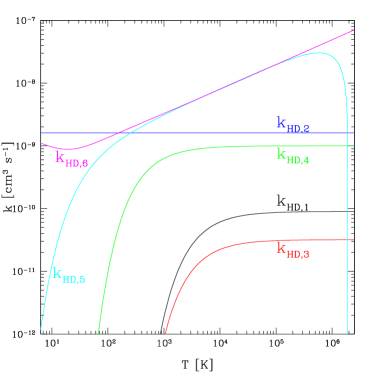
Figure 1: Temperature evolution of the reaction rates for deuterium chemistry. The labels refer to the number of the equation in the text.

For each species $i$, the variation in time of its number density $n_{i}$ is

$$\frac{\mathrm{d}n_{i}}{\mathrm{d}t}=\sum_{p}\sum_{q}k_{pq,i}n_{p}n_{q}-\sum_{l}k_{li}n_{l}n_{i},$$ (7)

where $k_{pq,i}$ in the first term on the right-hand side is the creation rate from species $p$ and $q$, and $k_{li}$ is the destruction rate from interactions of the species $i$ with the species $l$; they are temperature dependent and are usually expressed in $\rm[cm^{3}\,s^{-1}]$.
A plot of the rates as a function of the temperature is given in Figure 1, and the exact expressions and references in Appendix A. From the figure, it is clear that the most important reactions in the relevant range of temperatures are (5) and (6), and that the HD creation rates of reactions (1) and (2) are always higher than the corresponding destruction rates of reactions (3) and (4), respectively.

We have also considered $\rm HeH^{+}$ molecule evolution and found negligible effects on the cooling properties of the gas. The rates for $\rm HeH^{+}$ formation and destruction are given in Appendix A.

We implement our chemistry model extending the code by Yoshida et al. (2003), which adopts the rates from Abel et al. (1997), and modify it for self-consistency to obtain a set of reactions including e^-, H, H⁺, He, He⁺, He⁺⁺, H₂, H${}^{+}_{2}$, H^-, D, D⁺, HD, $\rm HeH^{+}$ (a complete list of the reactions is given in Table 1).
The set of differential equations (7) is evaluated via simple linearization, according to a backward difference formula (Anninos et al., 1997): given the time step $\Delta t$, at each time $t$ and for each species $i$, equation (7) can be re-written as

$$\frac{n_{i}^{t+\Delta t}-n_{i}^{t}}{\Delta t}=C_{i}^{t+\Delta t}-D_{i}^{t+\Delta t}n_{i}^{t+\Delta t}$$ (8)

where we have introduced the creation coefficient for the species $i$, in $\rm[cm^{-3}s^{-1}]$, as

$$C_{i}=\sum_{p}\sum_{q}k_{pq,i}n_{p}n_{q}$$ (9)

and the destruction coefficient, in $\rm[s^{-1}]$, as

$$D_{i}=\sum_{l}k_{li}n_{l}.$$ (10)

The number density, $n_{i}^{t}$, is then updated from equation (8):

$$n_{i}^{t+\Delta t}=\frac{C_{i}^{t+\Delta t}\Delta t+n_{i}^{t}}{1+D_{i}^{t+\Delta t}\Delta t}.$$ (11)

We apply this treatment to all chemical species.

Table 1: Set of reactions in the code.

Reactions	References for the rate coefficients
H + e- $\rightarrow$ H+ + 2e-	A97 / Y06
H+ + e- $\rightarrow$ H + $\gamma$	A97 / Y06
He + e- $\rightarrow$ He+ + 2e-	A97 / Y06
He+ + e- $\rightarrow$ He + $\gamma$	A97 / Y06
He+ + e- $\rightarrow$ He++ + 2e-	A97 / Y06
He++ + e- $\rightarrow$ He+ + $\gamma$	A97 / Y06
H + e- $\rightarrow$ H- + $\gamma$	A97 / Y06
H- + H $\rightarrow$ H2 + e-	A97 / Y06
H + H+ $\rightarrow$ H2+ + $\gamma$	A97 / Y06
H2+ + H $\rightarrow$ H2 + H+	A97 / Y06
H2 + H $\rightarrow$ 3H	A97
H2 + H+ $\rightarrow$ H2+ + H	S04 / Y06
H2 + e- $\rightarrow$ 2H + e-	ST99 / GB03 / Y06
H- + e- $\rightarrow$ H + 2e-	A97 / Y06
H- + H $\rightarrow$ 2H + e-	A97 / Y06
H- + H+ $\rightarrow$ 2H	P71 / GP98 / Y06
H- + H+ $\rightarrow$ H2+ + e-	SK87 / Y06
H2+ + e- $\rightarrow$ 2H	GP98 / Y06
H2+ + H- $\rightarrow$ H + H2	A97 / Y06
D + H2 $\rightarrow$ HD + H	WS02
D+ + H2 $\rightarrow$ HD + H+	WS02
HD + H $\rightarrow$ D + H2	SLP98
HD + H+ $\rightarrow$ D+ + H2	SLP98
H+ + D $\rightarrow$ H + D+	S02
H + D+ $\rightarrow$ H+ + D	S02
He + H+ $\rightarrow$ HeH+ + $\gamma$	RD82, GP98
HeH+ + H $\rightarrow$ He + H${}_{2}^{+}$	KAH79, GP98
HeH+ + $\gamma$ $\rightarrow$ He + H+	RD82, GP98

Notes - P71 = Peterson et al. (1971); KAH79 = Karpas et al. (1979); RD82 = Roberge & Dalgarno (1982); SK87 = Shapiro & Kang (1987); A97 = Abel et al. (1997); GP98 = Galli & Palla (1998); SLP98 = Stancil et al. (1998); ST99 = Stibbe & Tennyson (1999); WS02 = Wang & Stancil (2002); S02 = Savin (2002); GB03 = Glover & Brand (2003); S04 = Savin et al. (2004); Y06 = Yoshida et al. (2006).

2.2 Metal treatment at $\rm T<10^{4}~{}K$

For our calculations, we consider oxygen, carbon, silicon and iron, because they are the most abundant heavy atoms released during stellar evolution and, therefore, they play the most important role in chemical enrichment and cooling: indeed, supernovae type II (SNII) expel mostly oxygen and carbon, while supernovae type Ia (SNIa) silicon and iron (Thielemann et al., 2001; Park et al., 2003; Borkowski et al., 2004; Meynet et al., 2006).
We make the common assumption that carbon, silicon and iron are completely ionized, while oxygen is neutral. This is justified because, in a cosmological context, UV radiation below 13.6 eV (from various astrophysical sources, like quasars, stars, etc.) can escape absorption by neutral hydrogen and generate a UV background that can ionize atoms with first ionization potential lower than 13.6 eV (like carbon, silicon and iron). while oxygen remains predominantly neutral since its first ionization potential of 13.62 eV is higher (see also Bromm & Loeb, 2003; Santoro & Shull, 2006).

As in the low density regime of interest here thermodynamic equilibrium is never reached (see discussion of eq. 16), the Boltzmann distribution for the population of atomic levels can not be used. Thus, we will use the detailed balancing principle instead. For each level $i$ of a given species, we impose that the number of transitions to that level (which $populate$ it), per unit time and volume equals the number of transitions from the same level $i$ to other levels (which $de-populate$ it), per unit time and volume:

$$n_{i}\sum_{j}P_{ij}=\sum_{j}n_{j}P_{ji}\quad(i\neq j).$$ (12)

In formula (12), $P_{ij}$ is the probability per unit time of the transition $i\rightarrow j$ and $n_{i}$ and $n_{j}$ are the number densities of atoms in the $i$-th and $j$-th (with $i\neq j$) level. The left-hand side of the previous equation refers to de-populations of the $i$-th level, while the right-hand side refers to the transitions which can populate it.
The probability of a given transition can be easily computed once the Einstein coefficients and the collisional rates are known.
The further constraint which must be satisfied is the number particle conservation:

$$\sum_{j}n_{j}=n_{tot}$$ (13)

where $n_{tot}$ is the total number density of the species considered and $n_{j}$ the population of the generic level $j$.

In case of collisional events, the rate at which the transition $i\rightarrow j$ occurs is by definition:

$$n_{i}n_{x}\gamma_{ij}\equiv n_{i}n_{x}\langle u\sigma_{ij}\rangle=n_{i}n_{x}\int_{0}^{\infty}u\sigma_{ij}f(u)d^{3}u$$ (14)

where $\sigma_{ij}$ is the cross section of the process, $f(u)d^{3}u$ is the velocity distribution function of the particles (typically a Maxwellian), $\gamma_{ij}$ is the collisional rate, $n_{i}$ the number density of the particles in the $i$-th level and $n_{x}$ is the colliding particle number density.
The relation between $\gamma_{ij}$ and $\gamma_{ji}$ is:

$$g_{i}\gamma_{ij}=g_{j}\gamma_{ji}e^{-\beta\Delta E_{ji}},$$ (15)

where $g_{i}$ and $g_{j}$ are the level multiplicities, $\beta=(k_{B}T)^{-1}$, $\Delta E_{ji}$ is the energy level separation and $i<j$.
In addition to collisionally induced transitions, spontaneous transitions can take place with an emission rate given by the Einstein A coefficient.
It is convenient to define the critical number density for the transition $i\rightarrow j$ as

$$n_{cr,ij}=\frac{A_{ij}}{\gamma_{ij}}.$$ (16)

This determines the minimum density above which thermal equilibrium can be assumed and low density deviations from the Boltzmann distribution become irrelevant. At densities below $n_{cr,ij}$, we expect values of the excited level populations lower than in the thermodynamic limit, because of the reduced number of interactions.

For a two-level system, the low density level populations arising from electron and hydrogen impact excitations can be found by solving the system of equations resulting from conditions (13) and (12):

$$\left\{\begin{array}[]{l}\!\!\!\!n_{1}+n_{2}=n_{tot}\\ \\ \!\!\!\!n_{1}n_{H}\gamma_{12}^{H}\!+\!n_{1}n_{e}\gamma_{12}^{e}\!-\!n_{2}n_{H}\gamma_{21}^{H}\!-\!n_{2}n_{e}\gamma_{21}^{e}\!-\!n_{2}A_{21}\!=\!0\end{array}\right.$$ (17)

where $n_{H}$ and $n_{e}$ are the hydrogen and electron number density, while $\gamma_{12}^{H}$ and $\gamma_{12}^{e}$ are the H-impact and e-impact excitation rate.
The solution of (17) is:

$$\frac{n_{1}}{n_{tot}}=\frac{\gamma_{21}^{H}+\gamma_{21}^{e}n_{e}/n_{H}+A_{21}/n_{H}}{\gamma_{12}^{H}+\gamma_{21}^{H}+\left(\gamma_{12}^{e}+\gamma_{21}^{e}\right)n_{e}/n_{H}+A_{21}/n_{H}}$$ (18)

$$\frac{n_{2}}{n_{tot}}=\frac{\gamma_{12}^{H}+\gamma_{12}^{e}n_{e}/n_{H}}{\gamma_{12}^{H}+\gamma_{21}^{H}+\left(\gamma_{12}^{e}+\gamma_{21}^{e}\right)n_{e}/n_{H}+A_{21}/n_{H}}.$$ (19)

The ratio between the two level populations

$$\frac{n_{2}}{n_{1}} = \frac{\gamma_{12}^{H}+\gamma_{12}^{e}n_{e}/n_{H}}{\gamma_{21}^{H}+\gamma_{21}^{e}n_{e}/n_{H}+A_{21}/n_{H}}$$ (21)

$$\stackrel{{\scriptstyle n_{e}\ll n_{H}}}{{\sim}}\frac{\gamma_{12}^{H}}{\gamma_{21}^{H}+A_{21}/n_{H}}$$

will in general deviate from the Boltzmann statistic, because the spontaneous emission term dominates over the collisional term at low densities. In a neutral dense gas, instead, the level population saturates and simply reduces to a Boltzmann distribution, independently from the colliding particle number density.

In case of $n-$level systems, one must solve the $n\times n$ population matrix consisting of $n-1$ independent balancing equations (12) and the constraint of particle conservation (13).
In the modeling, we approximate CII and SiII as a two-level system, and OI and FeII as a five-level system (Santoro & Shull, 2006).
Further details on the atomic data and structures are reported in Appendix B.

2.3 Cooling

In addition to calculating the chemical evolution of the gas, we need to evaluate the cooling induced by different species. In the original code, hydrogen and helium cooling from collisional ionization, excitation and recombination (Hui & Gnedin, 1997), Compton cooling/heating and Bremsstrahlung (Black, 1981) are evaluated. For the H₂ and H${}_{2}^{+}$ cooling, the rates quoted in Galli & Palla (1998) are adopted. We take the HD cooling function from Lipovka et al. (2005), who consider the HD ro-vibrational structure and perform calculations for $J\leq 8$ rotational levels and $v=0,1,2,3$ vibrational levels. Their results are somehow more accurate than other approximations (Flower, 2000; Galli & Palla, 2002) and valid for a wide range of number densities (up to $\rm 10^{4}\,cm^{-3}$) and temperatures ($\rm 10^{2}~{}K-2\cdot 10^{4}~{}K$).
In Figure 2, we show cooling functions for H₂, HD, H${}_{2}^{+}$ molecules; for the latter case we distinguish between neutral hydrogen impact and electron impact cooling; we have assumed fractions x${}_{\rm HD}=10^{-8}$, x${}_{\rm H_{2}}=10^{-5}$, x${}_{\rm H_{2}^{+}}=10^{-13}$, x${}_{\rm e^{-}}=10^{-4}$ and a total hydrogen number density $\rm n_{H}=1\,cm^{-3}$. Due to its very low abundance, H${}_{2}^{+}$ is less effective than neutral H₂ and HD, which remain the only relevant coolants over the plotted range of temperature.
We highlight that the contribution of HD to gas cooling at low temperatures is dominant in the case considered here, but its relevance strongly depends on the relative abundances of the species.

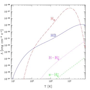
Figure 2: Cooling functions for a primordial gas with a hydrogen number density of $\rm 1\,cm^{-3}$ and the following fractions for the different species: x${}_{\rm HD}=10^{-8}$, x${}_{H_{2}}=10^{-5}$, x${}_{H_{2}^{+}}=10^{-13}$, x${}_{\rm e^{-}}=10^{-4}$. The $\rm H_{2}$ cooling function (long-dashed line) is plotted together with the HD (solid), H-impact $\rm H_{2}^{+}$ (dotted line) and e-impact $\rm H_{2}^{+}$ (short-dashed line) cooling functions. The fits for $\rm H_{2}^{+}$ cooling are appropriate only for $T<10^{4}$ K.

The cooling for metal line transitions is computed as follows. In case of two-level systems, we define

$$\Lambda\equiv n_{2}A_{21}\Delta E_{21}$$ (22)

where $n_{2}$ is the atomic excited state number density, $A_{21}$ is the probability per unit time of the transition $2\rightarrow 1$ and $\Delta E_{21}$ is the energy separation of the levels.

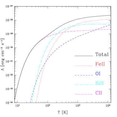
Figure 3: Cooling due to metals as a function of temperature. The computations are done for a gas with total number density of $\rm 1\,cm^{-3}$; for each metal species we assume a number density of $\rm 10^{-6}\,cm^{-3}$ and we set the free electron over hydrogen fraction to a value of $10^{-4}$.

Combining (22) and (19) one can write the previous equation as a function only of the total number density of the species

$$\Lambda\!\!=\!\!\frac{\gamma_{12}^{H}+\gamma_{12}^{e}n_{e}/n_{H}}{\gamma_{12}^{H}\!\!+\!\!\gamma_{21}^{H}\!\!+\!\!\left(\gamma_{12}^{e}\!\!+\!\!\gamma_{21}^{e}\right)n_{e}/n_{H}\!\!+\!\!A_{21}/n_{H}}n_{tot}A_{21}\Delta E_{21}.$$ (23)

For $n_{e}\ll n_{H}$, the previous formula is consistent with the one quoted in Santoro & Shull (2006), who do not consider electron impact excitation effects. Using equations (21) and (16), $\Lambda$ can also be written as a function of the fundamental level population

$$\Lambda = \frac{n_{1}n_{H}\gamma_{12}^{H}+n_{1}n_{e}\gamma_{12}^{e}}{n_{H}/n_{cr,21}^{H}+n_{e}/n_{cr,21}^{e}+1}\Delta E_{21}$$ (25)

$$\stackrel{{\scriptstyle n_{e}\ll n_{H}}}{{\sim}}\frac{n_{1}n_{H}\gamma_{12}^{H}}{n_{H}/n_{cr,21}^{H}+1}\Delta E_{21}$$

being $n_{cr,21}^{H}$ and $n_{cr,21}^{e}$ the critical density for the transition $2\rightarrow 1$ due to H- and e-impact excitations.
In particular, in the low density limit ($n_{H,e}\ll n_{cr}$), the above equation becomes

$$\Lambda\simeq \left[n_{1}n_{H}\gamma_{12}^{H}+n_{1}n_{e}\gamma_{12}^{e}\right]\Delta E_{21}\quad$$ (26)

$$\stackrel{{\scriptstyle n_{e}\ll n_{H}}}{{\sim}}n_{1}n_{H}\gamma_{12}^{H}\Delta E_{21}.$$ (27)

In this regime, each excitation - see formulae (26) and (27) - is statistically followed by emission of radiation - see the general definition (22).
In the high density limit, one finds the expected thermodynamic equilibrium cooling rate

$$\Lambda \simeq \frac{g_{2}}{g_{1}}e^{-\beta\Delta E_{21}}n_{1}\frac{A_{21}}{1+n_{e}\gamma_{21}^{e}/n_{H}\gamma_{21}^{H}}\Delta E_{21}+$$ (28)

$$\frac{g_{2}}{g_{1}}e^{-\beta\Delta E_{21}}n_{1}\frac{A_{21}}{1+n_{H}\gamma_{21}^{H}/n_{e}\gamma_{21}^{e}}\Delta E_{21}$$

$$\stackrel{{\scriptstyle n_{e}\ll n_{H}}}{{\sim}} \frac{g_{2}}{g_{1}}e^{-\beta\Delta E_{21}}n_{1}A_{21}\Delta E_{21}.$$ (29)

In the right-hand side, it is easy to recognize the Boltzmann distribution of populations for $n_{2}$. It is interesting to note that the cooling function does not depend any more on the number density of the colliding particles, but only on the species abundance, in contrast with the low density regime, where there is a linear dependence on both densities.
These arguments ensure that it is safe to use formula (23) to compute the gas cooling for two-level atoms.

For $n-$level systems, the cooling function is simply the sum of all the contributions from each transition

$$\Lambda\equiv\sum_{i\geq 1}\sum_{0\leq j<i}n_{i}A_{ij}\Delta E_{ij}.$$ (30)

In general, once the number density of the cooling species is fixed, we expect the cooling function to grow linearly with the colliding particle number density and eventually to saturate, converging to the Boltzmann statistic, when the critical densities are reached. We see that CII, SiII, FeII saturate when the colliding particle number density achieves values around $\rm 10^{4}\,cm^{-3}-10^{5}\,cm^{-3}$, while for OI we will have a double phase of saturation: the first one at $\rm\sim 10^{5}\,cm^{-3}$ involving the lower three states and the second one at $\rm\sim 10^{11}\,cm^{-3}$ involving the higher two states.

As an example, in Figure 3, we show the cooling functions for a total number density $\rm 1\,cm^{-3}$ and for each metal species $\rm 10^{-6}\,cm^{-3}$; the ratio between free electrons and hydrogen is chosen to be $\rm 10^{-4}$. With these values, the presence of electrons can affect the results up to $10\%$ with respect to the zero electron fraction case. We also notice that all the metals contribute with similar importance to the total cooling function and the main difference in the cooling properties of the gas will depend on their detailed chemical composition.

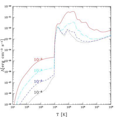
Figure 4: Total cooling due to hydrogen, helium, metals, H₂ and HD molecules as function of temperature, for gas having a hydrogen number density of 1 $\rm cm^{-3}$. The fraction of H₂ and HD are fixed to $10^{-5}$ and $10^{-8}$, respectively. The labels in the plot refer to different amount of metals, for individual metal number fractions of $10^{-3}$ (solid line), $10^{-4}$ (long-dashed line), $10^{-5}$ (short-dashed line) and $10^{-6}$ (dotted line).

We also plot the cooling functions for all the temperature regime we are interested in: at temperatures higher than $\rm 10^{4}~{}K$, we interpolate the Sutherland and Dopita tables (Sutherland & Dopita, 1993), at lower temperatures, we include metals and molecules as discussed previously. Figure 4 shows the cooling function for different individual metal number fractions with abundances in the range $10^{-6}-10^{-3}$ and $\rm H_{2}$ and HD fractions of $10^{-5}$ and $10^{-8}$, respectively. These values for $\rm H_{2}$ and HD are fairly typical for the IGM gas at the mean density (see also the conclusions of Galli & Palla, 1998, and references therein). In the temperature range $\rm 10^{4}~{}K-\rm 10^{5}~{}K$, the double peak due to hydrogen and helium collisional excitations is evident at low metallicity, while it is washed out by the contribution of different metal ionization processes as the metallicity increases. For example, complete collisional ionization of carbon and oxygen produces the twin peak at $\rm 10^{5}~{}K$, while complete ionization of iron is evident at about $\rm 10^{7}~{}K$. At temperatures lower than $10^{4}\rm~{}K$ and metal fractions lower than $\sim 10^{-6}$, the dominant cooling is given by molecules; instead, for larger metal fractions the effects of metals became dominant.
The general conclusion is that at very high redshift, when metals are not present, only $\rm H_{2}$ and HD can be useful to cool the gas down to some $\rm 10^{2}~{}K$, while after the first stars explode, ejecting heavy elements into the surrounding medium, metals quickly become the most efficient coolants.

3 Tests

In this section, we are going to test the implementation of HD and metal cooling using different kind of simulations. In particular, we focus on the analysis of abundance redshift evolution, cosmic structure formation and clusters.

3.1 Abundance redshift evolution

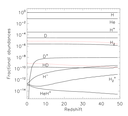
Figure 5: Abundances as a function of redshift. The solid lines refer to the abundance evolution in a flat cold dark matter universe with $h=~{}0.67$, $\rm\Omega_{0m}=~{}1$, $\rm\Omega_{0b}=~{}0.037$; the dotted lines refers to H₂ and HD evolution in a $\Lambda$CDM model with $h=~{}0.73$, $\rm\Omega_{0m}=~{}0.237$, $\rm\Omega_{0\Lambda}=~{}0.763$, $\rm\Omega_{0b}=~{}0.041$.

As a first test, we investigate the behavior of a plasma of primordial chemical composition (i.e. with no metals) looking at the redshift evolution of the single abundances. Our goal is to reproduce the results from Galli & Palla (1998), who calculate the redshift evolution of a metal-free gas at the mean density by following a detailed chemical network. For this reason, here, we perform our non-equilibrium computations on $isolated$ particles, including the following chemical species: e^-, H, H⁺, He, He⁺, He⁺⁺, H₂, H${}^{+}_{2}$, H^-, D, D⁺, HD, HeH⁺ and assuming a flat cosmology with no dark energy content (matter density parameter $\rm\Omega_{0m}=1$), baryon density parameter $\rm\Omega_{0b}=0.037$, Hubble constant, in units of $\rm 100km\,s^{-1}\,Mpc^{-1}$, $h=0.67$ and initial gas temperature of $1000\rm~{}K$.

The evolution of the number fractions for the different species is plotted in Figure 5; the electron abundance is given from charge conservation of neutral plasma and is normally very close to the $\rm H^{+}$ value, this being the dominant ion. These results are in very good agreement with those of Galli & Palla (1998).

In our set of reactions, due to the low initial gas temperature, the collisions are inefficient to ionize helium. The inclusion of $\rm HeH^{+}$ creation

$$\rm He+H^{+}\rightarrow HeH^{+}+\gamma$$ (31)

contributes to rise H${}_{2}^{+}$ abundance mainly via reaction

$$\rm HeH^{+}+H\rightarrow He+H_{2}^{+}$$ (32)

and weakly decrease the $\rm H^{-}$ number fraction via

$$\rm HeH^{+}+\gamma\rightarrow He+H^{+}$$ (33)

$$\rm H^{+}+H^{-}\rightarrow 2H$$ (34)

where $\gamma$ indicates the photons. Because of the very low $\rm HeH^{+}$ abundance reached, there is no substantial $\rm He$ atom abundance evolution.

Another $caveat$ to take into account is the lack of reactions between $\rm D^{+}$ and free electrons which would destroy the deuterium ions more efficiently, but without altering significantly the global amount of HD formed. We notice also the exponential decay of $\rm D^{+}$ due to the rate coefficient of equation (5) and the freezing out of $\rm H^{+}$, $\rm H_{2}$, D and HD number fractions.

As a comparison, we also plot (dotted lines) the H₂ and HD abundance evolution in a flat $\Lambda$CDM model having $h=~{}0.73$, $\rm\Omega_{0m}=0.237$, $\rm\Omega_{0\Lambda}=0.763$, $\rm\Omega_{0b}=0.041$ (Spergel et al. 2006). The slight increment observed is due to the fact that in the cold dark matter cosmology the baryon fraction is about $4\%$, making the interactions among different species rarer than in the $\Lambda$CDM model, for which the baryon fraction is about $17\%$. In addition, the cosmological constant is dominant only at redshifts below one. The evolution of the other species is similar in both cosmologies.

3.2 Cosmic structure formation

To test the behavior of the code in simulations of structure formation and evolution and the impact of HD, we run a cosmological simulation with the same properties and cosmology as in Maio et al. (2006). The main difference here is the addition of HD chemistry. We adopt the concordance $\rm\Lambda CDM$ model with $h=0.7$, $\rm\Omega_{0m}=0.3$, $\rm\Omega_{0b}=0.04$, $\rm\Omega_{0\Lambda}=0.7$; the power spectrum is normalized assuming a mass variance in a $\rm 8\,Mpc/h$ radius sphere $\sigma_{8}=0.9$ and the spectral index is chosen to be $\rm n=1$. We sample the cosmological field (in a periodic box of 1 Mpc comoving side length) with $324^{3}$ dark matter particles and the same number of gas particles, having a mass of about $\rm 1040\,M_{\odot}$ and $\rm 160\,M_{\odot}$, respectively. The comoving Plummer-equivalent gravitational softening length is fixed to $\rm 0.143\,kpc$. This allows to resolve halos with mass of about $10^{5}M_{\odot}$. The simulation starts at $z=90$ and is stopped at $z\sim$21.
We include the reactions involving e^-, H, H⁺, He, He⁺, He⁺⁺, H₂, H${}^{+}_{2}$, H^-, D, D⁺, HD (here we neglect $\rm HeH^{+}$, as it has not significant effects on the simulation) and compare the results with those of Maio et al. (2006), whose $\Lambda$CDM simulation has the same features, but the chemical set does not follow the evolution of D, D⁺ and HD and does not include $\rm H_{2}^{+}$ cooling.

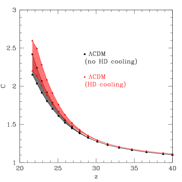
Figure 6: Gas clumping factor as a function of redshift for two $\rm\Lambda$CDM models with different chemical composition. The squares refer to the clumping factor computed with standard atomic line cooling and $\rm H_{2}$ cooling, while the triangles refer to a case which includes also HD cooling. The shaded regions correspond to the variation of the maximum overdensity between 100 (lower line in both cases) and 500 (upper line in both cases).

To quantify the differences between the two runs and the efficiency of the HD cooling we calculate the gas clumping factor, $C$, in the simulation box, in the following way

$$C=\frac{\sum_{i}m_{i}\rho_{i}\sum_{j}m_{j}\rho_{j}^{-1}}{\left(\sum_{k}m_{k}\right)^{2}}$$ (35)

where for each SPH particle, $i$, we indicate with $m_{i}$ its mass and with $\rho_{i}$ its mass density; the indices run over all the gas particles. For the sake of comparison, we calculate $C$ using only particles with density below a given overdensity threshold, $\delta_{M}$, and we make $\delta_{M}$ vary in the range [100, 500].
The results are plotted in Figure 6 for both simulations. We see that the inclusion of HD makes the clumping factor increase at all redshifts, almost independently from the density threshold. This means that the gas is, on average, denser and more clumped, with an increment of about 10% at redshift $\sim$22.

3.3 Cluster

So far, we have assumed either primordial gas with no metal pollution (previous test case) or a pre-defined metallicity to demonstrate the effect of the presence of metals on the cooling function at low temperature, as in Section 2.3. Now, we are going to couple our cooling function with a model for the chemical enrichment and test this implementation within a simulation that follows the formation of a cluster. In addition to testing the validity of our implementation, although there are no significant changes for the intra-cluster medium (ICM) to be expected, it is of interest to check whether there are regions inside the simulations where the polluted medium is cooling below $\rm 10^{4}~{}K$ due to its metal content.
The “zoomed initial condition technique” (Tormen et al., 1997) is used to extract from a dark matter-only simulation with box size of $\rm 479\,Mpc/h$ (we adopt a $\rm\Lambda CDM$ cosmology with $\rm H_{0}=~{}70\,km\,s^{-1}\,Mpc^{-1}$, $\sigma_{8}=~{}0.9$, $\rm\Omega_{0\Lambda}=~{}0.7$, $\rm\Omega_{0m}=~{}0.3$, $\rm\Omega_{0b}=~{}0.04$) a smaller region and to re-simulated it at higher resolution introducing also gas particles. The cluster evolution is simulated with about $2\cdot 10^{5}$ particles. The comoving Plummer-equivalent gravitational softening length is $\rm 5\,kpc/h$. At redshift zero, the selected cluster has a virial mass of about $\rm 10^{14}M_{\odot}/h$, a virial radius of about $\rm 1Mpc/h$ and a virial temperature of $2\cdot 10^{7}$  K (for more details see Dolag et al., 2004).
We start the simulation with no metallicity content. Then, the metal abundances are consistently derived (as in Tornatore et al., 2007) following the star formation history of the system, accounting for the lifetime of stars of different mass (Padovani & Matteucci, 1993) distributed according to a Salpeter IMF and adopting appropriated stellar yields: we use those from Woosley & Weaver (1995) for massive stars (SNII), van den Hoek & Groenewegen (1997) for low- and intermediate-mass stars and Thielemann et al. (2003) for SNIa. The underlying sub-resolution model for star formation in multi-phase interstellar medium (Springel & Hernquist, 2003) includes a phenomenological model for feedback from galactic ejecta powered by the SNII explosions, where we have chosen the wind velocity to be $\rm 480km\,s^{-1}$. As we are only interested to test the effect of the metals, we exclude H₂, HD and $\rm HeH^{+}$ chemistry and consider only atomic cooling from collisional excitations of hydrogen and helium. Once the medium gets polluted with metals, their contribution is added. For the metal cooling of the gas above $10^{4}$ K, Sutherland and Dopita tables (Sutherland & Dopita, 1993) are used. At lower temperatures, the fine structure transitions from OI, CII, SiII, FeII are included as discussed in the previous Sections.

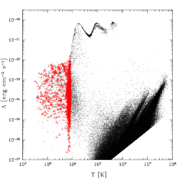
Figure 7: Distribution of the particles of a cluster simulation in the T-$\Lambda$ space. The hot and thin intra-cluster medium populates the bottom right area. The particles within collapsed objects, which represent very dense regions of the simulation, populate the high temperature cooling function (upper branch). In addition, metal enriched particles undergo metal line cooling in the low temperature regime (below $\sim 10^{4}$  K). The three-pointed star symbols correspond to particles which are located within twice the virial radius of the cluster and have a temperature lower than $\rm 8000~{}K$.

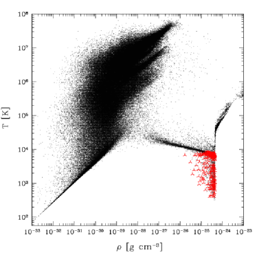
Figure 8: Distribution of the particles of a cluster simulation in the phase diagram. The hot and thin intra-cluster medium populates the central-left area of the plot, while the dense and cooled regions of the simulation are represented in the lower-right part. Particles heated by feedback effects are represented by points in the central-right side. The three-pointed star symbols correspond to metal enriched particles which are located within twice the virial radius of the cluster and have a temperature lower than $\rm 8000~{}K$. We remind that the critical density of the Universe at the present is $\rho_{0,cr}\simeq 1.9\cdot 10^{-29}h^{2}\quad g\,cm^{-3}$.

Figure 7 shows the cooling diagram of our simulation at redshift $z=0$; each SPH particle is represented by a point. In the plot, different areas can be identified. The one at high temperatures (bottom right) represents the hot ICM. When the ICM starts to get denser, cooling gets more efficient: the corresponding gas particles are represented by the points belonging to the upper branch of the cooling function and they are brought to lower and lower temperatures. Feedback from the star formation partially pushes some of them away from the cooling curve to slightly higher temperatures. Below $\rm 10^{4}~{}K$, only particles which are metal enriched can further cool down to about $\rm 300~{}K$, while gas particles with primordial composition are stacked at $\rm 10^{4}~{}K$. The three-pointed stars refer to particles within twice the virial radius and with a temperature below $\rm 8000~{}K$, indicating that this region of the T-$\Lambda$ space is also populated by gas associated with the galaxy cluster.
The corresponding phase diagram is shown in Figure 8. The three-pointed star symbols are the same as in Figure 7. The hot and thin intra-cluster medium populates the central-left area of the plot, while the dense and cool regions occupy the lower-right part. Particles heated by feedback are represented by points in the central-right side ($\rm\rho>~{}10^{-24}\,g\,cm^{-3}$, $\rm T>~{}10^{5}\,K$ ). The main effect of our metal cooling implementation is to lower the temperature of the dense medium, generating the sharp triangular area visible in the $\rm\rho~{}$-T space, at $\rm T<10^{4}~{}K$ and $\rm\rho~{}>~{}10^{-26}\,g\,cm^{-3}$. The points at very low densities are associated with diffuse metal free gas; this suggests that the spread in the cooling diagram of Figure 7 at temperature lower than $\rm 10^{4}~{}K$ is mainly due to different fractional metal enrichment of the particles, rather then to their different densities.
As already mentioned, global properties of the ICM and star formation are not significantly changed compared to the reference run without the metal line cooling from fine structure transitions. This happens because the simulation was merely meant to be a test case of the implementation of metal line cooling below $\rm 10^{4}~{}K$ under realistic conditions, but the halos resolved are large enough to cool and form stars without the aid of such cooling. In order to investigate in more detail the effects of the additional cooling by molecules and metals at low temperatures on the ICM and the star formation, higher resolution simulations are needed. However, this opens interesting grounds for further investigations on the interplay between formation of small objects, with virial temperatures in the range of interest for our extended cooling function, and metal pollution from first stars.

4 Conclusions

In order to understand structure formation and evolution, a detailed study of the chemical and cooling properties of baryonic matter is needed.
In this paper, we have presented time dependent calculations of the cooling properties of a gas in a “low temperature” regime, using the contributions of several chemical species and we have tested the effect on cosmic structure evolution.
Hydrogen derived molecules are effective in cooling metal-free gas below a temperature of $\rm\sim 10^{4}~{}K$, the typical temperature range of primordial objects. On the other hand, when the medium is polluted by material expelled from stars (via SN explosions, mass losses in AGB phase and winds), metals are expected to become the main coolants.
For these reasons, we have extended previous “non-equilibrium” calculations (Yoshida et al., 2003) in order to include in the numerical code Gadget-2 (Springel et al., 2001; Springel, 2005), the deuterium chemistry and follow the formation/destruction of HD molecule. This, together with molecular hydrogen, is able to cool down the gas at $\rm T~{}<~{}10^{4}~{}K$. Thanks to its permanent electric dipole moment, HD could allow cooling even below $\rm 10^{2}~{}K$ (Yoshida et al., 2006).
Other molecules are not very significant for the gas cooling properties.
The treatment of metal cooling at $\rm T\geq 10^{4}~{}K$ is included using the tables provided by Sutherland & Dopita (1993), while the contribution from fine structure transitions of oxygen, carbon, silicon and iron at $T<10^{4}$ K has been included by computing the populations of the levels, for each species, using the detailed balancing principle. More in particular, we have assumed that the UV radiation coming from the parent star ionizes carbon, silicon and iron, while oxygen remains neutral as its first ionization potential is higher than $\rm 13.6~{}eV$. We deal with the gas radiative losses computing the detailed balancing populations of the levels due to collisional excitations arising from hydrogen and electron impacts. The cooling follows the level de-excitations. The electron impact excitations are also included, as a residual electron fraction of about $10^{-4}$ survives in the post-recombination epoch and higher values are reached during the reionization process.
On the whole, we are now able to follow the evolution of e^-, H, H⁺, He, He⁺, He⁺⁺, H₂, H${}^{+}_{2}$, H^-, D, D⁺, HD, $\rm HeH^{+}$, O, C⁺, Si⁺, Fe⁺; so, the code is suitable to deal both with primordial and metal enriched gas.
We have checked the validity of our scheme by comparing the results of some test runs with previous calculations of molecule abundance evolution, finding excellent agreement.
We have also investigated the relevance of HD and metal cooling in some specific cases.
Adding the deuterium chemistry and HD contribution to the cooling function in simulations of structure formation results in a higher clumping factor of the gas, i.e. clouds are slightly denser and more compact, at high redshifts, with respect to the case when only H, He and $\rm H_{2}$ cooling is considered. The difference is about $10\%$ at $\rm z\sim 22$.
For what concerns the role of metal cooling at $\rm T<10^{4}~{}K$, we have shown that their presence is relevant in this temperature regime. In particular, in the cluster simulations we have run, fine structure transitions can actually cool the local temperature down to $\rm 10^{2}~{}K-10^{3}~{}K$.

In conclusion, we have implemented in Gadget-2, the most relevant features of gas cooling, in both pristine and polluted environments, for the temperature range $\rm 2.7~{}K-10^{9}~{}K$. We find that HD cooling has some influence on the high redshift gas clumping properties, while low temperature metal cooling has a significant impact on the formation and evolution of cold objects. In addition to investigating the above topics, this implementation can be used to study the detailed enrichment history of the IGM and its possible interplay with the transition between a primordial, massive star formation mode and a more standard one.

Appendix A Chemical rates

We consider the following set of equations involving HD creation and destruction:

$$\rm H_{2}\phantom{\,}+D\phantom{{}^{+}} \rightarrow \rm HD+H$$ (36)

$$\rm H_{2}\phantom{\,}+D^{+} \rightarrow \rm HD+H^{+}$$ (37)

$$\rm HD+H\phantom{{}^{+}} \rightarrow \rm D+H_{2}$$ (38)

$$\rm HD+H^{+} \rightarrow \rm D^{+}+H_{2}$$ (39)

$$\rm H^{+}+D\phantom{{}^{+}} \rightarrow \rm H+D^{+}$$ (40)

$$\rm H\phantom{{}^{+}}+D^{+} \rightarrow \rm H^{+}+D.$$ (41)

We use the rate coefficients from Wang & Stancil (2002):

$$k_{\rm HD,1} = 9.0\cdot 10^{-11}e^{-3876/T}\rm\,cm^{3}\,s^{-1}$$ (42)

$$k_{\rm HD,2} = 1.6\cdot 10^{-9}\rm cm^{3}s^{-1}$$ (43)

Stancil et al. (1998):

$$k_{\rm HD,3} = 3.2\cdot 10^{-11}e^{-3624/T}\rm\,cm^{3}\,s^{-1}$$ (44)

$$k_{\rm HD,4} = 10^{-9}e^{-464/T}\rm cm^{3}s^{-1}$$ (45)

and Savin (2002):

$$k_{\rm HD,5} \!\!\!\!\!\!=\!\!\!\!\!\! 2\!\!\cdot\!\!10^{-10}T^{0.402}e^{-37.1/T}\!\!-\!\!3.31\!\!\cdot\!\!10^{-17}T^{1.48}\rm cm^{3}s^{-1}$$ (46)

$$k_{\rm HD,6} \!\!\!\!\!\!\!\!=\!\!\!\!\!\!\!\! 2.06\!\!\cdot\!\!10^{-10}T^{0.396}\!e^{-33.0/T}\!\!\!\!+\!\!2.03\!\!\cdot\!\!10^{-9}T^{-0.332}\!\!\rm\,cm^{3}\,s^{-1}.$$ (47)

We consider the main equations for $\rm HeH^{+}$ formation and evolution (Galli & Palla, 1998), namely:

$$\rm He\phantom{-}+H^{+} \rightarrow \rm HeH^{+}+\gamma$$ (48)

$$\rm HeH^{+}+H \rightarrow \rm He+H_{2}^{+}$$ (49)

$$\rm HeH^{+}+\gamma \rightarrow \rm He+H^{+}$$ (50)

and the rates from Roberge & Dalgarno (1982):

$$k_{\rm HeH^{+},1}=\left\{\begin{array}[]{ll}\rm 7.6\cdot 10^{-18}T^{-0.5}\,cm^{3}\,s^{-1},&\rm T\leq 10^{3}~{}K\\ &\\ \rm 3.45\cdot 10^{-16}T^{-1.06}\,cm^{3}\,s^{-1},&\rm T>10^{3}~{}K\\ \end{array}\right.$$ (51)

Karpas et al. (1979):

$$k_{\rm HeH^{+},2}=9.1\cdot 10^{-10}\rm\,cm^{3}\,s^{-1}$$ (52)

and Roberge & Dalgarno (1982):

$$k_{\rm HeH^{+},3}=6.8\cdot 10^{-1}T_{r}^{1.5}e^{-22750/T_{r}}\rm\,s^{-1}.$$ (53)

In the previous expressions, $T$ stands for the gas temperature and $T_{r}$ for the radiation temperature.

Appendix B Atomic data

In the following, the atomic data adopted in this paper are provided (see also Osterbrock, 1989; Hollenbach & McKee, 1989; Santoro & Shull, 2006). We will use the usual spectroscopic notation for many electron atoms: S is the total electronic spin quantum operator, L the total electronic orbital angular momentum operator and J = L + S the sum operator; S, L, J, are the respective quantum numbers and X indicates the orbitals S, P, D, F, …, according to L=0, 1, 2, 3, …, respectively; then $\phantom{}{}^{2S+1}X_{J}$ will indicate the atomic orbital X, with spin quantum number S and total angular momentum quantum number J; its multiplicity is equal to $2J+1$.
In the following, we are going to discuss the models adopted for each species and the lines considered in a more detailed way.
We will often use the notation $\rm T_{100}=T/100~{}K$.

• CII: we model CII as a two-level system considering the fine structure transition $(2p)[\phantom{}^{2}P_{3/2}-\phantom{}^{2}P_{1/2}]$ between the quantum number $J=3/2$ and $J=1/2$ states. Data were taken from Hollenbach & McKee (1989):
  
  $\gamma_{21}^{H}=8\cdot 10^{-10}T_{100}^{0.07}\quad\rm cm^{3}\,s^{-1}$;
  $\gamma_{21}^{e}=2.8\cdot 10^{-7}T_{100}^{-0.5}\quad\rm cm^{3}\,s^{-1}$;
  $A_{21}=2.4\cdot 10^{-6}\quad\rm s^{-1}$;
  $\Delta E_{21}=1.259\cdot 10^{-14}\rm\,erg$ $\quad\rm(T_{exc}=91.2~{}K,\lambda=157.74\,\mu m)$.
  
  The cooling function is computed according to formula (23).
  

• SiII: we model SiII as a two-level system with the fine structure transition $(3p)[\phantom{}^{2}P_{3/2}-\phantom{}^{2}P_{1/2}]$. Data were taken from Hollenbach & McKee (1989):
  
  $\gamma_{21}^{H}=8\cdot 10^{-10}T_{100}^{-0.07}\quad\rm cm^{3}\,s^{-1}$;
  $\gamma_{21}^{e}=1.7\cdot 10^{-6}T_{100}^{-0.5}\quad\rm cm^{3}\,s^{-1}$;
  $A_{21}=2.1\cdot 10^{-4}\quad\rm s^{-1}$;
  $\Delta E_{21}=5.71\cdot 10^{-14}\,\rm\,erg$ $\quad\rm(T_{exc}=413.6~{}K,\lambda=34.8\,\mu m)$.
  
  The cooling function is computed following formula (23).
  

• OI: neutral oxygen is a metastable system formed by the (S=1, L=1) triplet and (S=0, L=0,2) doublet, $(2p)[\phantom{}^{3}P_{2}-\phantom{}^{3}P_{1}-\phantom{}^{3}P_{0}-\phantom{}^{1}D_{2}-\phantom{}^{1}S_{0}]$, in order of increasing level, with the following excitations rates (Hollenbach & McKee, 1989; Santoro & Shull, 2006):
  
  $\gamma^{H}_{21}=9.2\cdot 10^{-11}T_{100}^{0.67}\quad\rm cm^{3}\,s^{-1}$;
  $\gamma^{H}_{31}=4.3\cdot 10^{-11}T_{100}^{0.80}\quad\rm cm^{3}\,s^{-1}$;
  $\gamma^{H}_{32}=1.1\cdot 10^{-10}T_{100}^{0.44}\quad\rm cm^{3}\,s^{-1}$;
  $\gamma^{H}_{41}=\gamma^{H}_{42}=\gamma^{H}_{43}=10^{-12}\quad\rm cm^{3}\,s^{-1}$;
  $\gamma^{H}_{51}=\gamma^{H}_{52}=\gamma^{H}_{53}=10^{-12}\quad\rm cm^{3}\,s^{-1}$;
  $\gamma^{e}_{21}=1.4\cdot 10^{-8}\quad\rm cm^{3}\,s^{-1}$;
  $\gamma^{e}_{31}=1.4\cdot 10^{-8}\quad\rm cm^{3}\,s^{-1}$;
  $\gamma^{e}_{32}=5.0\cdot 10^{-9}\quad\rm cm^{3}\,s^{-1}$;
  $\gamma^{e}_{41}=\gamma^{e}_{42}=\gamma^{e}_{43}=10^{-10}\quad\rm cm^{3}\,s^{-1}$;
  $\gamma^{e}_{51}=\gamma^{e}_{52}=\gamma^{e}_{53}=10^{-10}\quad\rm cm^{3}\,s^{-1}$.
  
  The radiative transition probabilities are (Osterbrock, 1989; Hollenbach & McKee, 1989):
  
  $A_{21}=8.9\cdot 10^{-5}\quad\rm s^{-1}$;
  $A_{31}=1.0\cdot 10^{-10}\quad\rm s^{-1}$;
  $A_{32}=1.7\cdot 10^{-5}\quad\rm s^{-1}$;
  $A_{41}=6.3\cdot 10^{-3}\quad\rm s^{-1}$;
  $A_{42}=2.1\cdot 10^{-3}\quad\rm s^{-1}$;
  $A_{43}=7.3\cdot 10^{-7}\quad\rm s^{-1}$;
  $A_{51}=2.9\cdot 10^{-4}\quad\rm s^{-1}$;
  $A_{52}=7.3\cdot 10^{-2}\quad\rm s^{-1}$;
  $A_{54}=1.2\quad\rm s^{-1}$;
  
  energy separations are derived from Hollenbach & McKee (1989):
  
  $\Delta E_{21}=3.144\cdot 10^{-14}\,\rm erg$ $\quad\rm(T_{exc}=227.7~{}K,\lambda=63.18\,\mu m)$;
  $\Delta E_{32}=1.365\cdot 10^{-14}\,\rm erg$ $\quad\rm(T_{exc}=98.8~{}K,\lambda=145.5\,\mu m)$;
  $\Delta E_{43}=3.14\cdot 10^{-12}\,\rm erg$ $\quad\rm(T_{exc}=2.283\cdot 10^{4}~{}K,\lambda=6300\,\AA)$;
  $\Delta E_{53}=3.56\cdot 10^{-12}\,\rm erg$ $\quad\rm(T_{exc}=2.578\cdot 10^{4}~{}K,\lambda=5577\,\AA)$.
  
  To compute the cooling function, we solve for the five level populations and sum over the contributions from each of them.
  

• FeII: we adopt a model for a five-level system including the transitions $(3d)[\phantom{}^{6}D_{9/2}-\phantom{}^{6}D_{7/2}-\phantom{}^{6}D_{5/2}-\phantom{}^{6}D_{3/2}-\phantom{}^{6}D_{1/2}]$ in order of increasing level. For the data see also Santoro & Shull (2006) and references therein:
  
  $\gamma^{H}_{21}=9.5\cdot 10^{-10}\quad\rm cm^{3}\,s^{-1}$;
  $\gamma^{H}_{32}=4.7\cdot 10^{-10}\quad\rm cm^{3}\,s^{-1}$;
  $\gamma^{H}_{43}=5.\cdot 10^{-10}\quad\rm cm^{3}\,s^{-1}$;
  $\gamma^{H}_{54}=5\cdot 10^{-10}\quad\rm cm^{3}\,s^{-1}$;
  $\gamma^{H}_{31}=5.7\cdot 10^{-10}\quad\rm cm^{3}\,s^{-1}$;
  $\gamma^{H}_{41}=5\cdot 10^{-10}\quad\rm cm^{3}\,s^{-1}$;
  $\gamma^{H}_{51}=5\cdot 10^{-10}\quad\rm cm^{3}\,s^{-1}$;
  $\gamma^{H}_{42}=5\cdot 10^{-10}\quad\rm cm^{3}\,s^{-1}$;
  $\gamma^{H}_{52}=5\cdot 10^{-10}\quad\rm cm^{3}\,s^{-1}$;
  $\gamma^{H}_{53}=5\cdot 10^{-10}\quad\rm cm^{3}\,s^{-1}$;
  $\gamma^{e}_{21}=1.8\cdot 10^{-6}T_{100}^{-0.5}\quad\rm cm^{3}\,s^{-1}$;
  $\gamma^{e}_{32}=8.7\cdot 10^{-7}T_{100}^{-0.5}\quad\rm cm^{3}\,s^{-1}$;
  $\gamma^{e}_{43}=10^{-5}T^{-0.5}\quad\rm cm^{3}\,s^{-1}$;
  $\gamma^{e}_{54}=10^{-5}T^{-0.5}\quad\rm cm^{3}\,s^{-1}$;
  $\gamma^{e}_{31}=1.8\cdot 10^{-6}T_{100}^{-0.5}\quad\rm cm^{3}\,s^{-1}$;
  $\gamma^{e}_{41}=10^{-5}T^{-0.5}\quad\rm cm^{3}\,s^{-1}$;
  $\gamma^{e}_{51}=10^{-5}T^{-0.5}\quad\rm cm^{3}\,s^{-1}$;
  $\gamma^{e}_{42}=10^{-5}T^{-0.5}\quad\rm cm^{3}\,s^{-1}$;
  $\gamma^{e}_{52}=10^{-5}T^{-0.5}\quad\rm cm^{3}\,s^{-1}$;
  $\gamma^{e}_{53}=10^{-5}T^{-0.5}\quad\rm cm^{3}\,s^{-1}$;
  
  we assume a fiducial normalization of $10^{-5}$ for missing data on e-impact rates. We have checked that the level populations are almost insensitive to the adopted values.
  
  $A_{21}=2.13\cdot 10^{-3}\quad\rm s^{-1}$;
  $A_{32}=1.57\cdot 10^{-3}\quad\rm s^{-1}$;
  $A_{31}=1.50\cdot 10^{-9}\quad\rm s^{-1}$;
  $A_{43}=7.18\cdot 10^{-4}\quad\rm s^{-1}$;
  $A_{54}=1.88\cdot 10^{-4}\quad\rm s^{-1}$;
  
  $\Delta E_{21}=7.64\cdot 10^{-14}\rm\,erg$ $\quad\rm(T_{exc}=553.58~{}K,\lambda=25.99\,\mu m)$;
  $\Delta E_{32}=5.62\cdot 10^{-14}\rm\,erg$ $\quad\rm(T_{exc}=407.01~{}K,\lambda=35.35\,\mu m)$;
  $\Delta E_{43}=3.87\cdot 10^{-14}\rm\,erg$ $\quad\rm(T_{exc}=280.57~{}K,\lambda=51.28\,\mu m)$;
  $\Delta E_{54}=2.27\cdot 10^{-14}\rm\,erg$ $\quad\rm(T_{exc}=164.60~{}K,\lambda=87.41\,\mu m)$.
  
  To compute the cooling function, we solve for the five level populations and sum over the contributions from each of them.
  

A scheme of the atomic states, with wavelengths of the transitions between different levels, is given in Figure 9.

Figure 9: Scheme of the level models adopted for the different atoms with respective line transition data.

References

- Abel et al. (1997) Abel T., Anninos P., Zhang Y., Norman M. L., 1997, New Astronomy, 2, 181
- Abgrall & Roueff (2006) Abgrall H., Roueff E., 2006, A&A, 445, 361
- Abgrall et al. (1982) Abgrall H., Roueff E., Viala Y., 1982, A&A Supp., 50, 505
- Anninos et al. (1997) Anninos P., Zhang Y., Abel T., Norman M. L., 1997, New Astronomy, 2, 209
- Barkana & Loeb (2001) Barkana R., Loeb A., 2001, Phys. Rep., 349, 125
- Black (1981) Black J. H., 1981, MNRAS, 197, 553
- Borkowski et al. (2004) Borkowski K. J., Hendrick S. P., Reynolds S. P., 2004, in 35th COSPAR Scientific Assembly Vol. 35 of COSPAR, Plenary Meeting, Supernova ejecta in Magellanic Clouds remnants. pp 3560–+
- Bromm et al. (1999) Bromm V., Coppi P. S., Larson R. B., 1999, ApJ, 527, L5
- Bromm et al. (2002) Bromm V., Coppi P. S., Larson R. B., 2002, ApJ, 564, 23
- Bromm & Loeb (2003) Bromm V., Loeb A., 2003, Nature, 425, 812
- Burles & Tytler (1998) Burles S., Tytler D., 1998, ApJ, 507, 732
- Ciardi & Ferrara (2005) Ciardi B., Ferrara A., 2005, Space Science Reviews, 116, 625
- Dolag et al. (2004) Dolag K., Jubelgas M., Springel V., Borgani S., Rasia E., 2004, ApJ, 606, L97
- Flower (2000) Flower D. R., 2000, MNRAS, 318, 875
- Ford & Browne (1977) Ford A. L., Browne J. C., 1977, Phys. Rev. A, 16, 1992
- Frebel et al. (2007) Frebel A., Johnson J. L., Bromm V., 2007, ArXiv Astrophysics e-prints
- Galli & Palla (1998) Galli D., Palla F., 1998, A&A, 335, 403
- Galli & Palla (2002) Galli D., Palla F., 2002, P&SS, 50, 1197
- Glover & Brand (2003) Glover S. C. O., Brand P. W. J. L., 2003, MNRAS, 340, 210
- Gnedin (1998) Gnedin N. Y., 1998, MNRAS, 294, 407
- Hollenbach & McKee (1979) Hollenbach D., McKee C. F., 1979, ApJS, 41, 555
- Hollenbach & McKee (1989) Hollenbach D., McKee C. F., 1989, ApJ, 342, 306
- Hui & Gnedin (1997) Hui L., Gnedin N. Y., 1997, MNRAS, 292, 27
- Karlsson (2006) Karlsson T., 2006, ApJ, 641, L41
- Karpas et al. (1979) Karpas Z., Anicich V., Huntress Jr. W. T., 1979, J. Chem. Phys., 70, 2877
- Kawata & Gibson (2003) Kawata D., Gibson B. K., 2003, MNRAS, 340, 908
- Korn et al. (2006) Korn A. J., Grundahl F., Richard O., Barklem P. S., Mashonkina L., Collet R., Piskunov N., Gustafsson B., 2006, Nature, 442, 657
- Lepp & Shull (1984) Lepp S., Shull J. M., 1984, ApJ, 280, 465
- Lipovka et al. (2005) Lipovka A., Núñez-López R., Avila-Reese V., 2005, MNRAS, 361, 850
- Maio et al. (2006) Maio U., Dolag K., Meneghetti M., Moscardini L., Yoshida N., Baccigalupi C., Bartelmann M., Perrotta F., 2006, MNRAS, 373, 869
- McKellar et al. (1976) McKellar A. R. W., Goetz W., Ramsay D. A., 1976, ApJ, 207, 663
- Meynet et al. (2006) Meynet G., Ekström S., Maeder A., 2006, A&A, 447, 623
- Nakamura & Umemura (2002) Nakamura F., Umemura M., 2002, ApJ, 569, 549
- O’Meara et al. (2006) O’Meara J. M., Burles S., Prochaska J. X., Prochter G. E., Bernstein R. A., Burgess K. M., 2006, ApJ, 649, L61
- Osterbrock (1988) Osterbrock D. E., 1988, Publ. Astr. Soc. Pac., 100, 412
- Osterbrock (1989) Osterbrock D. E., 1989, Astrophysics of gaseous nebulae and active galactic nuclei. Mill Valley, CA, University Science Books, 1989, 422 p.
- Padovani & Matteucci (1993) Padovani P., Matteucci F., 1993, ApJ, 416, 26
- Park et al. (2003) Park S., Hughes J. P., Burrows D. N., Slane P. O., Nousek J. A., Garmire G. P., 2003, ApJ, 598, L95
- Peebles & Dicke (1968) Peebles P. J. E., Dicke R. H., 1968, ApJ, 154, 891
- Peterson et al. (1971) Peterson J. R., Aberth W. H., Moseley J. T., Sheridan J. R., 1971, Phys. Rev. A, 3, 1651
- Pettini & Bowen (2001) Pettini M., Bowen D. V., 2001, ApJ, 560, 41
- Puy et al. (1993) Puy D., Alecian G., Le Bourlot J., Leorat J., Pineau Des Forets G., 1993, A&A, 267, 337
- Raiteri et al. (1996) Raiteri C. M., Villata M., Navarro J. F., 1996, A&A, 315, 105
- Ricotti & Ostriker (2004) Ricotti M., Ostriker J. P., 2004, MNRAS, 350, 539
- Ripamonti (2007) Ripamonti E., 2007, ArXiv Astrophysics e-prints
- Roberge & Dalgarno (1982) Roberge W., Dalgarno A., 1982, ApJ, 255, 489
- Santoro & Shull (2006) Santoro F., Shull J. M., 2006, ApJ, 643, 26
- Saslaw & Zipoy (1967) Saslaw W. C., Zipoy D., 1967, Nature, 216, 976
- Savin (2002) Savin D. W., 2002, ApJ, 566, 599
- Savin et al. (2004) Savin D. W., Krstić P. S., Haiman Z., Stancil P. C., 2004, ApJ, 606, L167
- Schneider et al. (2003) Schneider R., Ferrara A., Salvaterra R., Omukai K., Bromm V., 2003, Nature, 422, 869
- Schneider et al. (2006) Schneider R., Omukai K., Inoue A. K., Ferrara A., 2006, MNRAS, 369, 1437
- Shapiro & Kang (1987) Shapiro P. R., Kang H., 1987, ApJ, 318, 32
- Shchekinov & Vasiliev (2006) Shchekinov Y. A., Vasiliev E. O., 2006, MNRAS, 368, 454
- Spitzer (1978) Spitzer L., 1978, Physical processes in the interstellar medium. New York Wiley-Interscience, 1978. 333 p.
- Springel (2005) Springel V., 2005, MNRAS, 364, 1105
- Springel & Hernquist (2003) Springel V., Hernquist L., 2003, MNRAS, 339, 289
- Springel et al. (2001) Springel V., Yoshida N., White S. D. M., 2001, New Astronomy, 6, 79
- Stancil et al. (1998) Stancil P. C., Lepp S., Dalgarno A., 1998, ApJ, 509, 1
- Stibbe & Tennyson (1999) Stibbe D. T., Tennyson J., 1999, ApJ, 513, L147
- Sutherland & Dopita (1993) Sutherland R. S., Dopita M. A., 1993, ApJS, 88, 253
- Thielemann et al. (2003) Thielemann F.-K., Argast D., Brachwitz F., Hix W. R., Höflich P., Liebendörfer M., Martinez-Pinedo G., Mezzacappa A., Panov I., Rauscher T., 2003, Nuclear Physics A, 718, 139
- Thielemann et al. (2001) Thielemann F.-K., Brachwitz F., Freiburghaus C., Rosswog S., Iwamoto K., Nakamura T., Nomoto K., Umeda H., Langanke K., Martinez-Pinedo G., Dean D. J., Hix W. R., Strayer M. S., 2001, in Livio M., Panagia N., Sahu K., eds, Supernovae and Gamma-Ray Bursts: the Greatest Explosions since the Big Bang Abundances from supernovae. pp 258–286
- Thorson et al. (1985) Thorson W. R., Choi J. H., Knudson S. K., 1985, Phys. Rev. A, 31, 22
- Tormen et al. (1997) Tormen G., Bouchet F. R., White S. D. M., 1997, MNRAS, 286, 865
- Tornatore et al. (2007) Tornatore L., Borgani S., Dolag K., Matteucci F., 2007, MNRASsubmitted, 0
- Tornatore et al. (2004) Tornatore L., Borgani S., Matteucci F., Recchi S., Tozzi P., 2004, MNRAS, 349, L19
- van den Hoek & Groenewegen (1997) van den Hoek L. B., Groenewegen M. A. T., 1997, A&A Supp., 123, 305
- Wang & Stancil (2002) Wang J. G., Stancil P. C., 2002, Physica Scripta Volume T, 96
- Woosley & Weaver (1995) Woosley S. E., Weaver T. A., 1995, ApJS, 101, 181
- Yong et al. (2006) Yong D., Carney B. W., Aoki W., McWilliam A., Schuster W. J., 2006, in Kubono S., Aoki W., Kajino T., Motobayashi T., Nomoto K., eds, AIP Conf. Proc. 847: Origin of Matter and Evolution of Galaxies Lithium Abundances in Halo Subgiants. pp 21–24
- Yoshida et al. (2003) Yoshida N., Abel T., Hernquist L., Sugiyama N., 2003, ApJ, 592, 645
- Yoshida et al. (2006) Yoshida N., Oh S. P., Kitayama T., Hernquist L., 2006, ArXiv Astrophysics e-prints
- Yoshida et al. (2006) Yoshida N., Omukai K., Hernquist L., Abel T., 2006, ApJ, 652, 6