A calculation of the shear viscosity in SU(3) gluodynamics

Abstract

We perform a lattice Monte-Carlo calculation of the two-point functions of the energy-momentum tensor at finite temperature in the SU(3) gauge theory. Unprecedented precision is obtained thanks to a multi-level algorithm. The lattice operators are renormalized non-perturbatively and the classical discretization errors affecting the correlators are corrected for. A robust upper bound for the shear viscosity to entropy density ratio is derived, $\eta/s<1.0$, and our best estimate is $\eta/s=0.134(33)$ at $T=1.65T_{c}$ under the assumption of smoothness of the spectral function in the low-frequency region.

Introduction.—   Models treating the system produced in heavy ion collisions at RHIC as an ideal fluid have had significant success in describing the observed flow phenomena huovinen ; shuryak . Subsequently the leading corrections due to a finite shear viscosity were computed teaney , in particular the flattening of the elliptic flow coefficient $v_{2}(p_{\rm T})$ above 1GeV. It is therefore important to compute the QCD shear and bulk viscosities from first principles to establish this description more firmly. Small transport coefficients are a signature of strong interactions, which lead to efficient transmission of momentum in the system. Strong interactions in turn require non-perturbative computational techniques. Several attempts have been made to compute these observables on the lattice in the SU(3) gauge theory karsch-visco ; nakamura . The underlying basis of these calculations are the Kubo formulas, which relate each transport coefficient to a spectral function $\rho(\omega)$ at vanishing frequency. Even on current computers, these calculations are highly non-trivial, due to the fall-off of the relevant correlators in Euclidean time (as $x_{0}^{-5}$ at short distances), implying a poor signal-to-noise ratio in a standard Monte-Carlo calculation. The second difficulty is to solve the ill-posed inverse problem for $\rho(\omega)$ given the Euclidean correlator at a finite set of points. Mathematically speaking, the uncertainty on a transport coefficient $\chi$ is infinite for any finite statistical accuracy, because adding $\epsilon\omega\delta(\omega)$ to $\rho(\omega)$ merely corresponds to adding a constant to the Euclidean correlator of order $\epsilon$, while rendering $\chi$ infinite. Therefore smoothness assumptions on $\rho(\omega)$ have to be made, which are reasonable far from the one-particle energy eigenstates, and can be proved in the hard-thermal-loop framework aarts .

In this Letter we present a new calculation which dramatically improves on the statistical accuracy of the Euclidean correlator relevant to the shear viscosity through the use of a two-level algorithm hm-ymills . This allows us to derive a robust upper bound on the viscosity and a useful estimate of the ratio $\eta/s$, which has acquired a special significance since its value $1/4\pi$ in a class of strongly coupled supersymmetric gauge theories policastro was conjectured to be an absolute lower bound for all substances kovtun .

Methodology.—   In the continuum, the energy-momentum tensor $\overline{T}_{\mu\nu}(x)=F_{\mu\alpha}^{a}F_{\nu\alpha}^{a}-{\textstyle\frac{1}{4}}\delta_{\mu\nu}F_{\rho\sigma}^{a}F_{\rho\sigma}^{a}$, being a set of Noether currents associated with translations in space and time, does not renormalize. With $L_{0}=1/T$ the inverse temperature, we consider the Euclidean two-point function ($0<x_{0}<L_{0}$)

$$C(x_{0})=L_{0}^{5}\int d^{3}{\bf x}~{}\langle\overline{T}_{12}(0)\overline{T}_{12}(x_{0},{\bf x})\rangle.$$ (1)

The tree-level expression is $C^{\rm t.l.}(x_{0})=\frac{32d_{A}}{5\pi^{2}}\Big{(}f(\tau)-\frac{\pi^{4}}{72}\Big{)}$, with $\tau=1-\frac{2x_{0}}{L_{0}}$, $d_{A}=8$ the number of gluons and $f(z)=\int_{0}^{\infty}ds~{}s^{4}\cosh^{2}(zs)/\sinh^{2}s$. The correlator $C(x_{0})$ is thus dimensionless and, in a conformal field theory, would be a function of $Tx_{0}$ only.

The spectral function is defined by

$$C(x_{0})=L_{0}^{5}\int_{0}^{\infty}\rho(\omega)\frac{\cosh\omega({\textstyle\frac{1}{2}}L_{0}-x_{0})}{\sinh\frac{\omega L_{0}}{2}}d\omega.$$ (2)

The shear viscosity is given by hosoya ; karsch-visco

$$\eta(T)=\pi\left.\frac{d\rho}{d\omega}\right|_{\omega=0}.$$ (3)

Important properties of $\rho$ are its positivity, $\rho(\omega)/\omega\geq 0$ and parity, $\rho(-\omega)=-\rho(\omega)$. The spectral function that reproduces $C^{\rm t.l.}(x_{0})$ is

$$\rho^{\rm t.l.}(\omega) = \frac{A_{\rm t.l.}~{}\omega^{4}}{\tanh{\textstyle\frac{1}{4}}\omega L_{0}}+BL_{0}^{-4}~{}\omega\delta(\omega),$$ (4)

$$A_{\rm t.l.} = \frac{1}{10}\frac{d_{A}}{(4\pi)^{2}},~{}~{}~{}~{}~{}B=\left(\frac{2\pi}{15}\right)^{2}~{}d_{A}.$$ (5)

While the $\omega^{4}$ term is expected to survive in the interacting theory with only logarithmic corrections, the $\delta$-function at the origin corresponds to the fact that gluons are asymptotic states in the free theory and implies an infinite viscosity.

On the lattice, translations only form a discrete group, so that a finite renormalization is necessary, $\overline{T}_{\mu\nu}(g_{0})=Z(g_{0})\overline{T}_{\mu\nu}^{\rm(bare)}.$ We employ the Wilson action wilson74 , $S_{\rm g}=\frac{1}{g_{0}^{2}}\sum_{x,\mu\neq\nu}{\rm Tr\,}\{1-P_{\mu\nu}(x)\}$, on an $L_{0}\cdot L^{3}$ hypertoroidal lattice, and the following discretized expression of the Euclidean energy:

$$\overline{T}_{00}^{\rm(bare)}(x)\equiv\frac{2}{a^{4}g_{0}^{2}}\Big{[}\sum_{k<l}\mathop{\rm Re}{\rm Tr\,}P_{kl}(x)-\sum_{k}\mathop{\rm Re}{\rm Tr\,}P_{0k}(x)\Big{]}$$

One of the lattice sum rules michael2 can be interpreted as a non-perturbative renormalization condition for this particular discretization, from which we read off $Z(g_{0})=1-{\textstyle\frac{1}{2}}g_{0}^{2}(c_{\sigma}-c_{\tau})$. The definition of the anisotropy coefficients $c_{\sigma,\tau}$ can be found in karsch-aniso , where they are computed non-perturbatively. With a precision of about $1\%$, a Padé fit constrained by the one-loop result karsch-pert yields

$$Z(g_{0})=\frac{1-1.0225g_{0}^{2}+0.1305g_{0}^{4}}{1-0.8557g_{0}^{2}},\quad(6/g_{0}^{2}\geq 5.7).$$ (6)

Numerical results.—   We report results obtained on a $\beta\equiv 6/g_{0}^{2}=6.2$, $8\cdot 20^{3}$ lattice and on a $\beta=6.408$, $8\cdot 28^{3}$ lattice. The first is thus at a temperature of $1.24T_{c}$, the second at $T=1.65T_{c}$. We use the results for $aT_{c}$ obtained in teper-sun and the non-perturbative lattice $\beta$-function of necco-sommer to determine this. We employ the two-level algorithm described in hm-ymills . The computing time invested into the $1.65T_{c}$ simulation is about 860 PC days. Following karsch-visco , we discretize ${\textstyle\frac{1}{4}}\langle(\overline{T}_{11}-\overline{T}_{22})(\overline{T}_{11}-\overline{T}_{22})\rangle$ instead of $\langle\overline{T}_{12}\overline{T}_{12}\rangle$ (the two are equal in the continuum) to write $C(x_{0})=\frac{L_{0}^{5}}{L^{3}}\langle O_{\eta}(0)O_{\eta}(x_{0})\rangle+{\rm O}(a^{2})$, where

$$O_{\eta}(x_{0})\equiv{\textstyle\frac{1}{2}}a^{3}\sum_{\bf x}\{\overline{T}_{11}-\overline{T}_{22}\}(g_{0},x)$$

$$=\frac{2Z(g_{0})}{a~{}g_{0}^{2}}~{}\sum_{\bf x}\mathop{\rm Re}{\rm Tr\,}\{P_{10}+P_{13}-P_{20}-P_{23}\}(x).$$

Figure 1: The correlators that contribute to $C(x_{0})={\textstyle\frac{1}{4}}(C_{BB}+C_{EE}+2C_{EB})$. Filled symbols correspond to $T=1.65T_{c}$, open symbols to $1.24T_{c}$. Error bars are smaller than the data symbols.

The three electric-electric, magnetic-magnetic and electric-magnetic contributions to $C(x_{0})$ are computed separately and shown on Fig. 1. We apply the following technique to remove the tree-level discretization errors sommer separately to $C_{BB},~{}C_{EE}$ and $C_{EB}$. Firstly, $\bar{x}_{0}$ is defined such that $C_{\rm cont}^{\rm t.l.}(\bar{x}_{0})=C_{\rm lat}^{\rm t.l.}(x_{0})$. The improved correlator is defined at a discrete set of points through $\overline{C}(\bar{x}_{0})=C(x_{0})$, and then augmented to a continuous function via $\overline{C}(\bar{x}_{0}^{(i)})=\alpha+\beta C_{\rm cont}^{\rm t.l.}(\bar{x}_{0}^{(i)})$, $i=1,2$, where $\bar{x}_{0}^{(1)}$ and $\bar{x}_{0}^{(2)}$ correspond to two adjacent measurements.

The resulting improved correlator, normalized by the continuum tree-level result, is shown on Fig. 2. One observes that the deviations from the tree-level result are surprisingly small, while deviations from conformality are visible. The latter is not unexpected at these temperatures, where $p/T^{4}$ is still strongly rising Boyd:1996bx . Finite-volume effects on the $T=1.65T_{c}$ lattice are smaller than one part in $10^{3}$ at tree-level. Non-perturbatively, at the same temperature with resolution $L_{0}/a=6$, increasing $L/a$ from 20 to 30 reduces $\overline{C}(L_{0}/2)$ by a factor 0.922(73). While not statistically compelling as it stands, the effect deserves further investigation.

Figure 2: The tree-level improved correlator $\overline{C}(x_{0})$ normalized to the tree-level continuum infinite-volume prediction. The four points in each sequence are strongly correlated, but their covariance matrix is non-singular.

The entropy density is obtained from the relation $s=(\epsilon+p)/T$ and the standard method to compute $\epsilon+p$ (karsch-aniso , Eq.1.14). We find $s/T^{3}=4.72(3)(5)$ and $5.70(2)(6)$ respectively at $T/T_{c}=1.24$ and $1.65$ (the first error is statistical and the second is the uncertainty on $Z(g_{0})$). The Stefan-Boltzmann value is $32\pi^{2}/45$ in the continuum and $1.0867$ times that value karsch-aniso at $L_{0}/a=8$.

Unsatisfactory attempts to extract the viscosity.—   In order to compare with previous studies karsch-visco ; nakamura , we fit $\overline{C}(x_{0})$ with a Breit-Wigner ansatz

$$\rho(\omega)/\omega=\frac{F}{1+b^{2}(\omega-\omega_{0})^{2}}+\frac{F}{1+b^{2}(\omega+\omega_{0})^{2}},$$ (7)

although it clearly ignores asymptotic freedom, which implies that $\rho(\omega)\sim\omega^{4}$ at $\omega\gg T$ aarts . The result of a correlated fit at $T=1.65T_{c}$ using the points at $Tx_{0}=0.5$, 0.35 and 0.275 is $a^{3}F=0.78(4)$, $(b/a)^{2}=240(30)$ and $a\omega_{0}=2.36(4)$, and hence $\eta/s|_{T=1.65T_{c}}=0.33(3)$. A comparison of this to the results of Ref. nakamura illustrates the progress made in statistical accuracy.

An ansatz motivated by the hard-thermal-loop framework is aarts

$$\rho(\omega)/\omega=\frac{\eta/\pi}{1+b^{2}\omega^{2}}+\theta(\omega-\omega_{1})\frac{A\omega^{3}}{\tanh\omega/4T}.$$ (8)

It is capable of reproducing the tree-level prediction, Eq. 4, and it allows for a thermal broadening of the delta function at the origin. Fitting the $T=1.65T_{c}$ points shown on Fig. 2, the $\chi^{2}$ is minimized for $b=0$ (effectively eliminating a free parameter), $A/A_{\rm t.l.}=0.996(8)$, $\omega_{1}/T=7.5(2)$ and $\eta/s=0.25(3)$, with $\chi^{2}_{\rm min}=4.0$. Thus while the ansatz is hardly compatible with the data, it shows that the data tightly constrains the coefficient $A$ to assume its tree-level value.

A bound on the viscosity.—   The positivity property of $\rho(\omega)$ allows us to derive an upper bound on the viscosity, based on the following assumptions:

1. the contribution to the correlator from $\omega>\Lambda$ is correctly predicted by the tree-level formula

2. the width of any potential peak in the region $\omega<T$ is no less than O($T$).

The standard QCD sum rule practice is to use perturbation theory from the energy lying midway between the lightest state and the first excitation. With this in mind we choose $\Lambda={\rm max}({\textstyle\frac{1}{2}}[M_{2}+M_{2^{*}}]\approx 2.6{\rm GeV},5T),$ where $M_{2^{(*)}}$ are the masses of the two lightest tensor glueballs. Perturbation theory predicts a Breit-Wigner centered at the origin of width $\Gamma=2\gamma$ aarts , where $\gamma\approx\alpha_{s}NT$ is the gluon damping rate. To derive the upper bound we conservatively assume that for $\omega<\sqrt{2}T$, $\rho(\omega)/\omega$ is a Breit-Wigner of width $\Gamma=T$ centered at the origin. From $C({\textstyle\frac{1}{2}}L_{0})\geq L_{0}^{5}\left[\int_{0}^{\sqrt{2}T}\rho_{BW}(\omega)+\int_{\Lambda}^{\infty}\rho_{\rm t.l.}(\omega)\right]\frac{d\omega}{\sinh\omega L_{0}/2}$ we obtain (with $90\%$ statistical confidence level)

$$\eta/s<\left\{\begin{array}[]{l@{~~~}l}0.96\hfil~{}~{}~{}&(T=1.65T_{c})\\ 1.08\hfil~{}~{}~{}&(T=1.24T_{c}).\end{array}\right.$$ (9)

The spectral function.—  

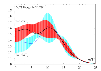
Figure 3: The result for $\rho(\omega)$. The meaning of the error bands and the curves is described in the text. The area under them equals $\overline{C}(L_{0}/2)=8.05(31)$ and 9.35(42) for $1.24T_{c}$ and $1.65T_{c}$ respectively.

As illustrated above, it is rather difficult to find a functional form for $\rho(\omega)$ that is both physically motivated and fits the data. In a more model-independent approach, $\rho(\omega)$ is expanded in an orthogonal set of functions, which grows as the lattice resolution on the correlator increases, and becomes complete in the limit of $L_{0}/a\to\infty$. We proceed to determine the function $\bar{\rho}(\omega)\equiv\rho(\omega)/\tanh({\textstyle\frac{1}{2}}\omega L_{0})$ by making the ansatz

$$\bar{\rho}(\omega)=m(\omega)~{}[1+a(\omega)],$$ (10)

where $m(\omega)>0$ has the high-frequency behavior of Eq. 4, and correspondingly define $\bar{K}(x_{0},\omega)=\cosh\omega(x_{0}-{\textstyle\frac{1}{2}}L_{0})/\cosh{\textstyle\frac{1}{2}}\omega L_{0}$. Suppose that $m(\omega)$ already is a smooth approximate solution to $\bar{\rho}(\omega)$; inserting (10) into (Eq. 2), one requires that $a(\omega)=\sum_{\ell}c_{\ell}a_{\ell}(\omega)$, with $\{a_{\ell}\}$ a basis of functions which is as sensitive as possible to the discrepancy between the lattice correlator and the correlator generated by $m(\omega)$. These are the eigenfunctions of largest eigenvalue of the symmetric kernel $G(\omega,\omega^{\prime})\equiv\int_{0}^{L_{0}}\frac{dx_{0}}{L_{0}}M(x_{0},\omega)M(x_{0},\omega^{\prime})$, where $M(x_{0},\omega)\equiv\bar{K}(x_{0},\omega)m(\omega)$. These functions satisfy $\int_{0}^{\infty}d\omega u_{\ell}(\omega)u_{\ell^{\prime}}(\omega)=\delta_{\ell\ell^{\prime}}$ and have an increasing number of nodes as their eigenvalue decreases. Thus the more data points available, the larger the basis and the finer details of the spectral function one is able to determine.

To determine the spectral function from $N$ points of the correlator, we proceed by first discretizing the $\omega$ variable into an $N_{\omega}$-vector. The final spectral function is given by the last member $\rho^{(N)}$ of a sequence whose first member is $\rho^{(0)}=m$ and whose general member $\rho^{(n)}$ reproduces $n$ points (or linear combinations) of the lattice correlator. For $n\geq 1$, $\rho^{(n)}=\rho^{(n-1)}[1+\sum_{\ell=1}^{n}c^{(n)}_{\ell}a^{(n)}_{\ell}]$ and the functions $a^{(n)}_{\ell}(\omega)$ are found by the SVD decomposition bryan of the $N_{\omega}\times n$ matrix $M^{(n)t}$, where $M_{ij}^{(n)}\equiv\bar{K}(x_{0}^{(i)},\omega_{j})\bar{\rho}^{(n-1)}(\omega_{j})$. The ‘model’ $m(\omega)$ is thus updated and agrees with $\rho(\omega)$ at the end of the procedure. We first performed this procedure on coarser lattices with $L_{0}/a=6$ at the same temperatures, starting from $m(\omega)=A_{\rm t.l.}\omega^{4}/(\tanh({\textstyle\frac{1}{4}}\omega L_{0})\tanh({\textstyle\frac{1}{2}}\omega L_{0})\tanh^{2}(c\omega L_{0}))$ with ${\textstyle\frac{1}{4}}\leq c\leq{\textstyle\frac{1}{2}}$, and then recycled the output as seed for the $L_{0}/a=8$ lattices. On the latter we used the $N=4$ points shown on Fig. 2.

The next question to address is the uncertainty on $\rho(\omega)$. It is important to realize that even in the absence of statistical errors, a systematic uncertainty subsists due to the finite number of basis functions we can afford to describe $\rho(\omega)$ with. A reasonable measure of this uncertainty is by how much $\rho(\omega)$ varies if one doubles the resolution on $C(x_{0})$. This can be estimated by ‘generating’ new points by using the computed $\rho^{(N)}(\omega)$. On the other hand we perform a two-point interpolation in $x_{0}$-space (we chose the form $(\alpha+\beta(x_{0}-{\textstyle\frac{1}{2}}L_{0})^{2})/\sin^{5}(\pi x_{0}/L_{0})$), and take the difference between these and the generated ones as their systematic uncertainty. In practice this difference is added in quadrature with the statistical uncertainty. Next we repeat the procedure to find $\rho$ described above with $N\to 2N$: if we use as seed $\rho^{(N)}$, then by construction it is left invariant by the iterative procedure, but the derivatives of $\rho^{(2N)}$ with respect to the $2N$ points of the correlator can be evaluated. The error on $\rho(\omega)$ is then obtained from a formula of the type $(\delta\rho)^{2}=\sum_{i=1}^{2N}(\frac{\partial\rho}{\partial C_{i}})^{2}(\delta C_{i})^{2}$ which however keeps track of correlations in $x_{0}$ and Monte-Carlo time. This is the error band shown on Fig. 3 and the corresponding shear viscosity values are

$$\eta/s=\left\{\begin{array}[]{l@{~~~}l}0.134(33)\hfil~{}~{}~{}&(T=1.65T_{c})\\ 0.102(56)\hfil~{}~{}~{}&(T=1.24T_{c}).\end{array}\right.$$ (11)

It is also interesting to check for the stability of the solution under the use of a larger basis of functions. If instead of starting from $\rho^{(N)}(\omega)$ we restart from $\rho^{(0)}$ (the output of the $L_{0}/a=6$ lattice) and fit the $2N$ (dependent) points using $2N$ basis functions $\{a_{\ell}\}$, we obtain the curves drawn on Fig. 3. As one would hope, the oscillations of $\rho^{(2N)}(\omega)$ are covered by the error band.

Conclusion.—   Using state-of-the-art lattice techniques, we have computed the correlation functions of the energy-momentum tensor to high accuracy in the SU(3) pure gauge theory. We have calculated the leading high-temperature cutoff effects and removed them from the correlator relevant to the shear viscosity, and we normalized it non-perturbatively, exploiting existing results. We obtained the entropy density with an accuracy of $1\%$. The most robust result obtained on the shear viscosity is the upper bound Eq. (9), which comes from lumping the area under the curve on Fig. 3 in the interval $[0,6T]$ into a peak of width $\Gamma=T$ centered at the origin. Secondly, our best estimate of the shear viscosity is given by Eq. (11), using a new method of extraction of the spectral function. The errors contain an estimate of the systematic uncertainty associated with the limited resolution in Euclidean time. We are extending the calculation to finer lattice spacings and larger volumes to further consolidate our findings.

The values (11) are intriguingly close to saturating the KSS bound kovtun $\eta/s\geq 1/4\pi$. We note that in perturbation theory the ratio $\eta/s$ does not depend strongly on the number of quark flavors arnold . Our results thus corroborate the picture of a near-perfect fluid that has emerged from the RHIC experiments, with the magnitude of the anisotropic flow incompatible with $\eta/s\gtrsim 0.2$ teaney .

Acknowledgments.—   I thank Krishna Rajagopal and Philippe de Forcrand for their encouragement and many useful discussions. This work was supported in part by funds provided by the U.S. Department of Energy under cooperative research agreement DE-FC02-94ER40818.

References

- (1) P. F. Kolb, P. Huovinen, U. W. Heinz and H. Heiselberg, Phys. Lett. B 500, 232 (2001); P. Huovinen, P. F. Kolb, U. W. Heinz, P. V. Ruuskanen and S. A. Voloshin, Phys. Lett. B 503, 58 (2001).
- (2) D. Teaney, J. Lauret and E. V. Shuryak, Phys. Rev. Lett. 86, 4783 (2001).
- (3) D. Teaney, Phys. Rev. C 68, 034913 (2003).
- (4) F. Karsch and H.W. Wyld, Phys. Rev. D 35, 2518 (1987).
- (5) A. Nakamura and S. Sakai, Phys. Rev. Lett. 94, 072305 (2005).
- (6) G. Aarts and J.M. Martinez Resco, JHEP 0204, 053 (2002).
- (7) G. Policastro, D.T. Son and A.O. Starinets, Phys. Rev. Lett. 87, 081601 (2001).
- (8) P. Kovtun, D.T. Son and A.O. Starinets, Phys. Rev. Lett. 94, 111601 (2005).
- (9) K.G. Wilson, Phys. Rev. D 10, 2445 (1974).
- (10) C. Michael, Phys. Rev. D 53 (1996) 4102.
- (11) F. Karsch, Nucl. Phys. B 205, 285 (1982).
- (12) J. Engels, F. Karsch and T. Scheideler, Nucl. Phys. B 564 (2000) 303 [arXiv:hep-lat/9905002].
- (13) A. Hosoya, M.A. Sakagami and M. Takao, Annals Phys. 154, 229 (1984).
- (14) B. Lucini, M. Teper and U. Wenger, JHEP 0401, 061 (2004).
- (15) S. Necco and R. Sommer, Nucl. Phys. B 622 (2002) 328.
- (16) H.B. Meyer, JHEP 0401, 030 (2004).
- (17) R. Sommer, Nucl. Phys. B 411 (1994) 839.
- (18) G. Boyd, J. Engels, F. Karsch, E. Laermann, C. Legeland, M. Lutgemeier and B. Petersson, Nucl. Phys. B 469, 419 (1996).
- (19) R.K. Bryan, Eur. Biophys. J., 18 (1990) 165.
- (20) P. Arnold, G.D. Moore and L.G. Yaffe, JHEP 0305, 051 (2003).