Phenomenology with Massive Neutrinos

Abstract

The current status and some perspectives of the phenomenology of massive neutrinos is reviewed. We start with the phenomenology of neutrino oscillations in vacuum and in matter. We summarize the results of neutrino experiments using solar, atmospheric, reactor and accelerator neutrino beams. We update the leptonic parameters derived from the three-neutrino oscillation interpretation of this data. We describe the method and present results on our understanding of the solar and atmospheric neutrino fluxes by direct extraction from the corresponding neutrino event rates. We present some tests of different forms of new physics which induce new sources of leptonic flavor transitions in vacuum and in matter which can be performed with the present neutrino data. The aim and potential of future neutrino experiments and facilities to further advance in these fronts is also briefly summarized. Last, the implications of the LSND observations are discussed, and the status of extended models which could accommodate all flavor-mixing signals is presented in the light of the recent results from MiniBooNE.

It is already five decades since the first neutrino was observed by Cowan and Reines [1] in 1956 in a reactor experiment, and more than seventy five years since its existence was postulated by Wolfgang Pauli [2], in 1930, in order to reconcile the observed continuous spectrum of nuclear beta decay with energy conservation. It has been a long and winding road that has lead us from these pioneering times to the present overwhelming proof that neutrinos are massive and leptonic flavors are not symmetries of Nature. A road in which both theoretical boldness and experimental ingenuity have walked hand by hand to provide us with the first evidence of physics beyond the Standard Model [3]. From the desperate solution of Pauli to the cathedral-size detectors built to capture and study in detail the elusive particle.

Neutrinos are copiously produced in natural sources: in the burning of the stars, in the interaction of cosmic rays…even as relics of the Big Bang. Starting from the 1960’s, neutrinos produced in the sun and in the atmosphere were observed. In 1987, neutrinos from a supernova in the Large Magellanic Cloud were also detected. Indeed an important leading role in this story was played by the neutrinos produced in the sun and in the atmosphere. The experiments that measured the flux of atmospheric neutrinos found results that suggested the disappearance of muon-neutrinos when propagating over distances of order hundreds (or more) kilometers. Experiments that measured the flux of solar neutrinos found results that suggested the disappearance of electron-neutrinos while propagating within the Sun or between the Sun and the Earth.

These results called back to 1968 when Gribov and Pontecorvo [4, 5] realized that flavor oscillations arise if neutrinos are massive and mixed. The disappearance of both atmospheric $\nu_{\mu}$’s and solar $\nu_{e}$’s was most easily explained in terms of neutrino oscillations. The emerging picture was that at least two neutrinos were massive and mixed, unlike what it is predicted in the Standard Model.

In the last decade this picture became fully established with the upcome of a set of precise experiments. In particular, during the last five years the results obtained with solar and atmospheric neutrinos have been confirmed in experiments using terrestrial beams in which neutrinos produced in nuclear reactors and accelerators facilities have been detected at distances of the order of hundred kilometers.

Neutrinos were introduced in the Standard Model as truly massless fermions, for which no gauge invariant renormalizable mass term can be constructed. Consequently, in the Standard Model there is neither mixing nor CP violation in the leptonic sector. Therefore, the experimental evidence for neutrino masses and mixing provided an unambiguous signal of new physics.

At present the phenomenology of massive neutrinos is in a very interesting moment. On the one hand many extensions of the Standard Model anticipated ways in which neutrinos may have small, but definitely non-vanishing masses. The better determination of the flavor structure of the leptons at low energies is of vital importance as, at present, it is our only source of positive information to pin-down the high energy dynamics implied by the neutrino masses. Needless to say that its potential will be further expanded and complemented if a positive signal on the absolute value of the mass scale is observed in kinematic searches or or in neutrinoless double beta decay as well as if the observations from a positive evidence in the precision cosmological data.

However as we stand now, even the minimal picture of three massive neutrino, although satisfactory, is still not complete. We do not have direct evidence of one of the three mixing angles and we are far from a precise determination of the other two. Also, although oscillations have allowed us to establish that neutrinos have mass, they do not probe their absolute mass scale. Finally, we ignore if there is CP violation in the leptonic sector, and we do not know if neutrinos are their own antiparticle. Different experiments have been proposed and several techniques are being explored to answer all these fundamental questions.

On the other hand, the attained precision in the observed signals is already good enough to allow us the use of the existing data to probe physics beyond neutrino masses and mixings. In particular it is possible to test more exotic neutrino properties and/or interactions which can induce new sources of leptonic flavor mixing and affect the established oscillation pattern. Also the independent determination of neutrino masses and mixing in experiments performed with terrestrial beams opens up the possibility of testing the theoretical predictions of the natural neutrino fluxes, produced either in the Sun or in the atmosphere, directly from the corresponding neutrino data.

The purpose of this review is to quantitatively summarize the present status of the phenomenology of massive neutrinos on some of these fronts. In Sec. 1 we present the low energy formalism for adding neutrino masses to the SM and the induced leptonic mixing, and then we describe the phenomenology associated with neutrino oscillations in vacuum and in matter. In Sec. 2 we briefly summarize the present experimental results from solar, atmospheric, reactor and accelerator neutrinos, as independently as possible of any particle physics interpretation. Section 3 contains an update of the three-neutrino oscillation interpretation of the existing bulk of neutrino data (with the exception of the LSND result). Section 4 describes the method and present results of test of our understanding of the solar and atmospheric neutrino fluxes by direct extraction from the corresponding neutrino data. Sections 5 and 6 are devoted to tests of different forms of new physics which induce new sources of leptonic flavor transitions in vacuum and in matter and which can be performed with the present neutrino data. The aim and potential of future neutrino experiments and facilities to further advance in these fronts is briefly summarized in Sec. 7. In Sec. 8 we describe the status of the existing probes to the absolute neutrino mass scale. For years the most troublesome piece of experimental evidence in neutrino physics was that of the LSND experiment which observed a small appearance of electron anti-neutrinos in a muon anti-neutrino beam at a value of $L/E$ different from that of either solar and atmospheric neutrinos. Very recently, the MiniBooNE experiment has presented their negative results on the search for $\nu_{\mu}\rightarrow\nu_{e}$ oscillations in the same $L/E$ region. In Sec. 9 we describe the extensions proposed to accommodate the LSND result and discuss their phenomenological status in the light of the recent MiniBooNE result. Our conclusions are summarized in Sec. 10. This review is complemented by an Appendix in which we update the details of the atmospheric neutrino analysis presented in this report.

The field of neutrino phenomenology and its forward-looking perspectives is rapidly evolving. The overview presented in this review is only partial and lacks of many aspects. For other excellent reviews see Refs. [6, 7, 3, 8, 9, 10, 11, 12, 13, 14, 15] and the books [16, 17, 18, 19, 20, 21, 22]. An exhaustive list of related references can be found in Ref. [14].

1 Neutrino Masses and Mixing

The greatest success of modern particle physics has been the establishment of the connection between forces mediated by spin-1 particles and local (gauge) symmetries. Within the Standard Model, the strong, weak and electromagnetic interactions are connected to, respectively, $SU(3)$, $SU(2)$ and $U(1)$ gauge groups. The characteristics of the different interactions are explained by the symmetry to which they are related. For example, the way in which the fermions exert and experience each of the forces is determined by their representation under the corresponding symmetry group (or simply their charges in the case of Abelian gauge symmetries).

Once the gauge invariance is elevated to the level of fundamental physics principle, it must be verified by all terms in the Lagrangian, including the mass terms. This, as we will see, has important implications for the neutrino.

1.1 Standard Model of Massless Neutrinos

The Standard Model (SM) is based on the gauge group

$$G_{\text{SM}}=SU(3)_{\text{C}}\times SU(2)_{\text{L}}\times U(1)_{\text{Y}},$$ (1)

with three matter fermion generations. Each generation consists of five different representations of the gauge group:

$$\left(1,2,-\frac{1}{2}\right),\quad\left(3,2,\frac{1}{6}\right),\quad\left(1,1,-1\right),\quad\left(3,1,\frac{2}{3}\right),\quad\left(3,1,-\frac{1}{3}\right)$$ (2)

where the numbers in parenthesis represent the corresponding charges under the group (1). In this notation the electric charge is given by

$$Q_{\text{EM}}=T_{L3}+Y\,.$$ (3)

The matter content is shown in Table 1, and together with the corresponding gauge fields it constitutes the full list of fields required to describe the observed elementary particle interactions. In fact, these charge assignments have been tested to better than the percent level for the light fermions [23]. The model also contains a single Higgs boson doublet, $\phi$ with charges $(1,2,1/2)$, whose vacuum expectation value breaks the gauge symmetry,

$$\langle\phi\rangle=\begin{pmatrix}0\\ \frac{v}{\sqrt{2}}\end{pmatrix}\quad\Longrightarrow\quad G_{\text{SM}}\rightarrow SU(3)_{\text{C}}\times U(1)_{\text{EM}}.$$ (4)

This is the only piece of the SM model which still misses experimental confirmation. Indeed, the search for the Higgs boson, remains one of the premier tasks of present and future high energy collider experiments.

Table 1: Matter contents of the SM.

$L_{L}(1,2,-\frac{1}{2})$	$Q_{L}(3,2,\frac{1}{6})$	$E_{R}(1,1,-1)$	$U_{R}(3,1,\frac{2}{3})$	$D_{R}(3,1,-\frac{1}{3})$
$\begin{pmatrix}\nu_{e}\\[-5.69054pt] e\end{pmatrix}_{L}$	$\begin{pmatrix}u\\[-5.69054pt] d\end{pmatrix}_{L}$	$e_{R}$	$u_{R}$	$d_{R}$
$\begin{pmatrix}\nu_{\mu}\\[-5.69054pt] \mu\end{pmatrix}_{L}$	$\begin{pmatrix}c\\[-5.69054pt] s\end{pmatrix}_{L}$	$\mu_{R}$	$c_{R}$	$s_{R}$
$\begin{pmatrix}\nu_{\tau}\\[-5.69054pt] \tau\end{pmatrix}_{L}$	$\begin{pmatrix}t\\[-5.69054pt] b\end{pmatrix}_{L}$	$\tau_{R}$	$t_{R}$	$b_{R}$

As can be seen in Table 1 neutrinos are fermions that have neither strong nor electromagnetic interactions (see Eq. (3)), i.e. they are singlets of $SU(3)_{\text{C}}\times U(1)_{\text{EM}}$. We will refer as active neutrinos to neutrinos that, such as those in Table 1, reside in the lepton doublets, that is, that have weak interactions. Conversely sterile neutrinos are defined as having no SM gauge interactions (their charges are $(1,1,0)$), that is, they are singlets of the full SM gauge group.

The SM has three active neutrinos accompanying the charged lepton mass eigenstates, $e$, $\mu$ and $\tau$, thus there are weak charged current (CC) interactions between the neutrinos and their corresponding charged leptons given by

$$-{\mathcal{L}}_{\text{CC}}=\frac{g}{\sqrt{2}}\sum_{\ell}\bar{\nu}_{L\ell}\gamma^{\mu}\ell^{-}_{L}W_{\mu}^{+}+\text{h.c.}.$$ (5)

In addition, the SM neutrinos have also neutral current (NC) interactions,

$$-{\mathcal{L}}_{\text{NC}}=\frac{g}{2\cos\theta_{W}}\sum_{\ell}\bar{\nu}_{L\ell}\gamma^{\mu}\nu_{L\ell}Z_{\mu}^{0}.$$ (6)

The SM as defined in Table 1, contains no sterile neutrinos.

Thus, within the SM, Eqs. (5) and (6) describe all the neutrino interactions. From Eq. (6) one can determine the decay width of the $Z^{0}$ boson into neutrinos which is proportional to the number of light (that is, $m_{\nu}\leq m_{Z}/2$) left-handed neutrinos. At present the measurement of the invisible Z width yields $N_{\nu}=2.984\pm 0.008$ [23] which implies that whatever the extension of the SM we want to consider, it must contain three, and only three, light active neutrinos.

An important feature of the SM, which is relevant to the question of the neutrino mass, is the fact that the SM with the gauge symmetry of Eq. (1) and the particle content of Table 1 presents an accidental global symmetry:

$$G_{\text{SM}}^{\text{global}}=U(1)_{B}\times U(1)_{L_{e}}\times U(1)_{L_{\mu}}\times U(1)_{L_{\tau}}.$$ (7)

$U(1)_{B}$ is the baryon number symmetry, and $U(1)_{L_{e},L_{\mu},L_{\tau}}$ are the three lepton flavor symmetries, with total lepton number given by $L=L_{e}+L_{\mu}+L_{\tau}$. It is an accidental symmetry because we do not impose it. It is a consequence of the gauge symmetry and the representations of the physical states.

In the SM, fermions masses arise from the Yukawa interactions which couple a right-handed fermion with its left-handed doublet and the Higgs field,

$$-\mathcal{L}_{\text{Yukawa}}=Y^{d}_{ij}\bar{Q}_{Li}\phi D_{Rj}+Y^{u}_{ij}\bar{Q}_{Li}\tilde{\phi}U_{Rj}+Y^{\ell}_{ij}\bar{L}_{Li}\phi E_{Rj}+\text{h.c.},$$ (8)

(where $\tilde{\phi}=i\tau_{2}\phi^{\star}$) which after spontaneous symmetry breaking lead to charged fermion masses

$$m^{f}_{ij}=Y^{f}_{ij}\frac{v}{\sqrt{2}}\,.$$ (9)

However, since no right-handed neutrinos exist in the model, the Yukawa interactions of Eq. (8) leave the neutrinos massless.

In principle neutrino masses could arise from loop corrections. In the SM, however, this cannot happen because the only possible neutrino mass term that can be constructed with the SM fields is the bilinear $\bar{L}_{L}L^{C}_{L}$ which violates the total lepton symmetry by two units. As mentioned above total lepton number is a global symmetry of the model and therefore $L$-violating terms cannot be induced by loop corrections. Furthermore, the $U(1)_{B-L}$ subgroup of $G_{\text{SM}}^{\text{global}}$ is non-anomalous. and therefore $B-L$-violating terms cannot be induced even by nonperturbative corrections.

It follows that the SM predicts that neutrinos are precisely massless. In order to add a mass to the neutrino the SM has to be extended.

1.2 Introducing Massive Neutrinos

As discussed above, with the fermionic content and gauge symmetry of the SM one cannot construct a renormalizable mass term for the neutrinos. So in order to introduce a neutrino mass one must either extend the particle contents of the model or abandon gauge invariance and/or renormalizability.

In what follows we illustrate the different types of neutrino mass terms by assuming that we keep the gauge symmetry and we explore the possibilities that we have to introduce a neutrino mass term if one adds to the SM an arbitrary number $m$ of sterile neutrinos $\nu_{si}(1,1,0)$.

With the particle contents of the SM and the addition of an arbitrary $m$ number of sterile neutrinos one can construct two types mass terms that arise from gauge invariant renormalizable operators:

$$-\mathcal{L}_{M_{\nu}}={M_{D}}_{ij}\bar{\nu}_{si}\nu_{Lj}+\frac{1}{2}{M_{N}}_{ij}\bar{\nu}_{si}\nu^{c}_{sj}+\text{h.c.}.$$ (10)

Here $\nu^{c}$ indicates a charge conjugated field, $\nu^{c}=C\bar{\nu}^{T}$ and $C$ is the charge conjugation matrix. $M_{D}$ is a complex $m\times 3$ matrix and $M_{N}$ is a symmetric matrix of dimension $m\times m$.

The first term is a Dirac mass term. It is generated after spontaneous electroweak symmetry breaking from Yukawa interactions

$$Y^{\nu}_{ij}\bar{\nu}_{si}\tilde{\phi}^{\dagger}L_{Lj}\Rightarrow{M_{D}}_{ij}=Y^{\nu}_{ij}\frac{v}{\sqrt{2}}$$ (11)

similarly to the charged fermion masses. It conserves total lepton number but it breaks the lepton flavor number symmetries.

The second term in Eq. (10) is a Majorana mass term. It is different from the Dirac mass terms in many important aspects. It is a singlet of the SM gauge group. Therefore, it can appear as a bare mass term. Furthermore, since it involves two neutrino fields, it breaks lepton number by two units. More generally, such a term is allowed only if the neutrinos carry no additive conserved charge.

In general Eq. (10) can be rewritten as:

$$-\mathcal{L}_{M_{\nu}}=\frac{1}{2}\overline{\vec{\nu}^{c}}M_{\nu}\vec{\nu}+\text{h.c.}\,,$$ (12)

where

$$M_{\nu}=\begin{pmatrix}0&M^{T}_{D}\\ M_{D}&M_{N}\end{pmatrix},$$ (13)

and $\vec{\nu}=(\vec{\nu}_{L},\,\vec{\nu^{c}_{s}})^{T}$ is a $(3+m)$-dimensional vector. The matrix $M_{\nu}$ is complex and symmetric. It can be diagonalized by a unitary matrix of dimension $(3+m)$, $V^{\nu}$, so that

$$({V^{\nu}})^{T}M_{\nu}{V^{\nu}}=\mathop{\mathrm{diag}}(m_{1},m_{2},\dots,m_{3+m})\,.$$ (14)

In terms of the resulting $3+m$ mass eigenstates

$$\vec{\nu}_{\text{mass}}=({V^{\nu}})^{\dagger}\vec{\nu}\,,$$ (15)

Eq. (12) can be rewritten as:

$$-\mathcal{L}_{M_{\nu}}=\frac{1}{2}\sum_{k=1}^{3+m}m_{k}\left(\bar{\nu}^{c}_{\text{mass},k}\nu_{\text{mass},k}+\bar{\nu}_{\text{mass},k}\nu^{c}_{\text{mass},k}\right)=\frac{1}{2}\sum_{k=1}^{3+m}m_{k}\bar{\nu}_{Mk}\nu_{Mk}\,,$$ (16)

where

$$\nu_{Mk}=\nu_{\text{mass},k}+\nu^{c}_{\text{mass},k}=({V^{\nu}}^{\dagger}\vec{\nu})_{k}+({V^{\nu}}^{\dagger}\vec{\nu})^{c}_{k}$$ (17)

which obey the Majorana condition

$$\nu_{M}=\nu_{M}^{c}$$ (18)

and are refereed to as Majorana neutrinos. Notice that this condition implies that there is only one field which describes both neutrino and antineutrino states. Thus a Majorana neutrino can be described by a two-component spinor unlike the charged fermions, which are Dirac particles, and are represented by four-component spinors.

From Eq. (17) we find that the weak-doublet components of the neutrino fields are:

$$\nu_{Li}=L\,\sum_{j=1}^{3+m}V^{\nu}_{ij}\nu_{Mj}\quad{i=1,3}\,,$$ (19)

where $L$ is the left-handed projector.

In the rest of this section we will discuss three interesting cases.

1.2.1 $M_{N}=0$: Dirac Neutrinos

Forcing $M_{N}=0$ is equivalent to imposing lepton number symmetry on the model. In this case, only the first term in Eq. (10), the Dirac mass term, is allowed. For $m=3$ we can identify the three sterile neutrinos with the right-handed component of a four-spinor neutrino field. In this case the Dirac mass term can be diagonalized with two $3\times 3$ unitary matrices, $V^{\nu}$ and $V^{\nu}_{R}$ as:

$${V^{\nu}_{R}}^{\dagger}M_{D}V^{\nu}=\mathop{\mathrm{diag}}(m_{1},m_{2},m_{3})\,.$$ (20)

The neutrino mass term can be written as:

$$-\mathcal{L}_{M_{\nu}}=\sum_{k=1}^{3}m_{k}\bar{\nu}_{Dk}\nu_{Dk}$$ (21)

where

$${\nu_{D}}_{k}=({V^{\nu}}^{\dagger}\vec{\nu}_{L})_{k}+({V^{\nu}_{R}}^{\dagger}\vec{\nu}_{s})_{k}\,,$$ (22)

so the weak-doublet components of the neutrino fields are

$$\nu_{Li}=L\sum_{j=1}^{3}V^{\nu}_{ij}\nu_{Dj}\,,\qquad i=1,3\,.$$ (23)

Let’s point out that in this case the SM is not even a good low-energy effective theory since both the matter content and the assumed symmetries are different. Furthermore there is no explanation to the fact that neutrino masses happen to be much lighter than the corresponding charged fermion masses as in this case all acquire their mass via the same mechanism.

1.2.2 $M_{N}\gg M_{D}$: The see-saw mechanism

In this case the scale of the mass eigenvalues of $M_{N}$ is much higher than the scale of electroweak symmetry breaking $\langle\phi\rangle$. The diagonalization of $M_{\nu}$ leads to three light, $\nu_{l}$, and $m$ heavy, $N$, neutrinos:

$$-\mathcal{L}_{M_{\nu}}=\frac{1}{2}\bar{\nu}_{l}M^{l}\nu_{l}+\frac{1}{2}\bar{N}M^{h}{N}$$ (24)

with

$$M^{l}\simeq-V_{l}^{T}M_{D}^{T}M_{N}^{-1}M_{D}V_{l},\qquad M^{h}\simeq V_{h}^{T}M_{N}V_{h}$$ (25)

and

$$V^{\nu}\simeq\begin{bmatrix}\left(1-\frac{1}{2}M_{D}^{\dagger}{M^{*}_{N}}^{-}1M_{N}^{-1}M_{D}\right)V_{l}&M_{D}^{\dagger}{M^{*}_{N}}^{-1}V_{h}\\ -M_{N}^{-1}M_{D}V_{l}&\left(1-\frac{1}{2}{M_{N}}^{-1}M_{D}M_{D}^{\dagger}{M^{*}_{N}}^{-1}\right)V_{h}\end{bmatrix}$$ (26)

where $V_{l}$ and $V_{h}$ are $3\times 3$ and $m\times m$ unitary matrices respectively. So the heavier are the heavy states, the lighter are the light ones. This is the see-saw mechanism [24, 25, 26, 27, 28]. Also as seen from Eq. (26) the heavy states are mostly right-handed while the light ones are mostly left-handed. Both the light and the heavy neutrinos are Majorana particles. Two well-known examples of extensions of the SM that lead to a see-saw mechanism for neutrino masses are SO(10) GUTs [25, 26, 27] and left-right symmetry [28].

In this case the SM is a good effective low energy theory. Indeed the see-saw mechanism is a particular realization of the general case of a full theory which leads to the SM with three light Majorana neutrinos as its low energy effective realization as we discuss next.

1.2.3 Neutrino Masses from Non-renormalizable Operators

In general, if the SM is an effective low energy theory valid up to the scale $\Lambda_{\text{NP}}$, the gauge group, the fermionic spectrum, and the pattern of spontaneous symmetry breaking of the SM are still valid ingredients to describe Nature at energies $E\ll\Lambda_{\text{NP}}$. But because it is an effective theory, one must also consider non-renormalizable higher dimensional terms in the Lagrangian whose effect will be suppressed by powers $1/\Lambda_{\text{NP}}^{\text{dim-4}}$. In this approach the largest effects at low energy are expected to come from dim$=5$ operators.

There is no reason for generic NP to respect the accidental symmetries of the SM (7). Indeed, there is a single set of dimension-five terms that is made of SM fields and is consistent with the gauge symmetry, and this set violates (7). It is given by

$$\mathcal{O}_{5}=\frac{Z^{\nu}_{ij}}{\Lambda_{\text{NP}}}{\left(\bar{L}_{Li}\tilde{\phi}\right)}{\left({\tilde{\phi}}^{T}L^{C}_{Lj}\right)}+\text{h.c.},$$ (27)

which violate total lepton number by two units and leads, upon spontaneous symmetry breaking, to:

$$-\mathcal{L}_{M_{\nu}}=\frac{Z^{\nu}_{ij}}{2}\frac{v^{2}}{\Lambda_{\text{NP}}}\bar{\nu}_{Li}\nu^{c}_{Lj}+\text{h.c.}\,.$$ (28)

Comparing with Eq. (12) we see that this is a Majorana mass term built with the left-handed neutrino fields and with:

$$(M_{\nu})_{ij}={Z^{\nu}_{ij}}\frac{v^{2}}{\Lambda_{\text{NP}}}.$$ (29)

Since Eq. (29) would arise in a generic extension of the SM, we learn that neutrino masses are very likely to appear if there is NP. As mentioned above, a theory with SM plus $m$ heavy sterile neutrinos leads to three light mass eigenstates and an effective low energy interaction of the form (27). In particular, the scale $\Lambda_{\text{NP}}$ is identified with the mass scale of the heavy sterile neutrinos, that is the typical scale of the eigenvalues of $M_{N}$.

Furthermore, comparing Eq. (29) and Eq. (9), we find that the scale of neutrino masses is suppressed by $v/\Lambda_{\text{NP}}$ when compared to the scale of charged fermion masses providing an explanation not only for the existence of neutrino masses but also for their smallness. Finally, Eq. (29) breaks not only total lepton number but also the lepton flavor symmetry $U(1)_{e}\times U(1)_{\mu}\times U(1)_{\tau}$. Therefore, as we shall see in Sec. 1.3, we should expect lepton mixing and CP violation unless additional symmetries are imposed on the coefficients $Z_{ij}$.

1.2.4 Light sterile neutrinos

This appears if the scale of some eigenvalues of $M_{N}$ is not higher than the electroweak scale. As in the case with $M_{N}=0$, the SM is not even a good low energy effective theory: there are more than three light neutrinos, and they are admixtures of doublet and singlet fields. Again both light and heavy neutrinos are Majorana particles.

As we will see the analysis of neutrino oscillations is the same whether the light neutrinos are of the Majorana- or Dirac-type. From the phenomenological point of view, only in the discussion of neutrinoless double beta decay the question of Majorana versus Dirac neutrinos is crucial. However, as we have tried to illustrate above, from the theoretical model building point of view, the two cases are very different.

1.3 Lepton Mixing

The possibility of arbitrary mixing between two massive neutrino states was first introduced in Ref. [29]. In the general case, we denote the neutrino mass eigenstates by $(\nu_{1},\nu_{2},\nu_{3},\dots,\nu_{n})$ and the charged lepton mass eigenstates by $(e,\mu,\tau)$. The corresponding interaction eigenstates are denoted by $(e^{I},\mu^{I},\tau^{I})$ and $\vec{\nu}=(\nu_{Le},\nu_{L\mu},\nu_{L\tau},\nu_{s1},\dots,\nu_{sm})$. In the mass basis, leptonic charged current interactions are given by

$$-\mathcal{L}_{\text{CC}}=\frac{g}{\sqrt{2}}(\bar{e}_{L},\,\bar{\mu}_{L},\,\bar{\tau}_{L})\gamma^{\mu}U\begin{pmatrix}\nu_{1}\\ \nu_{2}\\ \nu_{3}\\ \vdots\\ \nu_{n}\end{pmatrix}W_{\mu}^{+}-\text{h.c.}.$$ (30)

Here $U$ is a $3\times n$ matrix [30, 31, 32] which verifies

$$UU^{\dagger}=I_{3\times 3}$$ (31)

but in general $U^{\dagger}U\neq I_{n\times n}$.

The charged lepton and neutrino mass terms and the neutrino mass in the interaction basis are:

$$-{\mathcal{L}}_{M}=[(\bar{e}_{L}^{I},\,\bar{\mu}_{L}^{I},\,\bar{\tau}_{L}^{I})M_{\ell}\begin{pmatrix}e_{R}^{I}\\ \mu_{R}^{I}\\ \tau_{R}^{I}\end{pmatrix}+\text{h.c.}]-\mathcal{L}_{M_{\nu}}$$ (32)

with $\mathcal{L}_{M_{\nu}}$ given in Eq. (12). One can find two $3\times 3$ unitary diagonalizing matrices for the charge leptons, $V^{\ell}$ and $V^{\ell}_{R}$, such that

$${V^{\ell}}^{\dagger}M_{\ell}V^{\ell}_{R}=\mathop{\mathrm{diag}}(m_{e},m_{\mu},m_{\tau})\,.$$ (33)

The charged lepton mass term can be written as:

$$-\mathcal{L}_{M_{\ell}}=\sum_{k=1}^{3}m_{\ell_{k}}\bar{\ell}_{k}\ell_{k}$$ (34)

where

$$\ell_{k}=({V^{\ell}}^{\dagger}\ell^{I}_{L})_{k}+({V^{\ell}_{R}}^{\dagger}\ell^{I}_{R})_{k}$$ (35)

so the weak-doublet components of the charge lepton fields are

$$\ell^{I}_{Li}=L\,\sum_{j=1}^{3}V^{\ell}_{ij}\ell_{j}\,,\qquad i=1,3$$ (36)

From Eqs. (19), (23) and (36) we find that $U$ is:

$$U_{ij}=P_{\ell,ii}\,{V^{\ell}_{ik}}^{\dagger}\,V^{\nu}_{kj}\,(P_{\nu,jj}).$$ (37)

$P_{\ell}$ is a diagonal $3\times 3$ phase matrix, that is conventionally used to reduce by three the number of phases in $U$. $P_{\nu}$ is a diagonal $n\times n$ phase matrix with additional arbitrary phases which can chosen to reduce the number of phases in $U$ by $n-1$ only for Dirac states. For Majorana neutrinos, this matrix is simply a unit matrix. The reason for that is that if one rotates a Majorana neutrino by a phase, this phase will appear in its mass term which will no longer be real. Thus, the number of phases that can be absorbed by redefining the mass eigenstates depends on whether the neutrinos are Dirac or Majorana particles. Altogether for Majorana [Dirac] neutrinos the $U$ matrix contains a total of $6(n-2)$ [$5n-11$] real parameters, of which $3(n-2)$ are angles and $3(n-2)$ [$2n-5$] can be interpreted as physical phases.

In particular, if there are only three Majorana neutrinos, $U$ is a $3\times 3$ matrix analogous to the CKM matrix for the quarks [33] but due to the Majorana nature of the neutrinos it depends on six independent parameters: three mixing angles and three phases. In this case the mixing matrix can be conveniently parametrized as:

$$U=\begin{pmatrix}1&0&0\\ 0&c_{23}&{s_{23}}\\ 0&-s_{23}&{c_{23}}\end{pmatrix}\cdot\begin{pmatrix}c_{13}&0&s_{13}e^{-i\delta_{\text{CP}}}\\ 0&1&0\\ -s_{13}e^{i\delta_{\text{CP}}}&0&c_{13}\end{pmatrix}\cdot\begin{pmatrix}c_{21}&s_{12}&0\\ -s_{12}&c_{12}&0\\ 0&0&1\end{pmatrix}\cdot\begin{pmatrix}e^{i\eta_{1}}&0&0\\ 0&e^{i\eta_{2}}&0\\ 0&0&1\end{pmatrix},$$ (38)

where $c_{ij}\equiv\cos\theta_{ij}$ and $s_{ij}\equiv\sin\theta_{ij}$. The angles $\theta_{ij}$ can be taken without loss of generality to lie in the first quadrant, $\theta_{ij}\in[0,\pi/2]$ and the phases $\delta_{\text{CP}},\;\eta_{i}\in[0,2\pi]$. This is to be compared to the case of three Dirac neutrinos, where the Majorana phases, $\eta_{1}$ and $\eta_{2}$, can be absorbed in the neutrino states and therefore the number of physical phases is one (similarly to the CKM matrix). In this case the mixing matrix $U$ takes the form [23]:

$$U=\begin{pmatrix}c_{12}\,c_{13}&s_{12}\,c_{13}&s_{13}\,e^{-i\delta_{\text{CP}}}\\ -s_{12}\,c_{23}-c_{12}\,s_{13}\,s_{23}\,e^{i\delta_{\text{CP}}}&\hphantom{+}c_{12}\,c_{23}-s_{12}\,s_{13}\,s_{23}\,e^{i\delta_{\text{CP}}}&c_{13}\,s_{23}\hskip 15.649pt\\ \hphantom{+}s_{12}\,s_{23}-c_{12}\,s_{13}\,c_{23}\,e^{i\delta_{\text{CP}}}&-c_{12}\,s_{23}-s_{12}\,s_{13}\,c_{23}\,e^{i\delta_{\text{CP}}}&c_{13}\,c_{23}\hskip 15.649pt\end{pmatrix}.$$ (39)

Note, however, that the two extra Majorana phases are very hard to measure since they are only physical if neutrino mass is non-zero and therefore the amplitude of any process involving them is suppressed a factor $m_{\nu}/E$ to some power where $E$ is the energy involved in the process which is typically much larger than the neutrino mass. The most sensitive experimental probe of Majorana phases is the rate of neutrinoless $\beta\beta$ decay.

If no new interactions for the charged leptons are present we can identify their interaction eigenstates with the corresponding mass eigenstates after phase redefinitions. In this case the charged current lepton mixing matrix $U$ is simply given by a $3\times n$ sub-matrix of the unitary matrix $V^{\nu}$.

It worth noticing that while for the case of 3 light Dirac neutrinos the procedure leads to a fully unitary $U$ matrix for the light states, generically for three light Majorana neutrinos this is not the case when the full spectrum contains heavy neutrino states which have been integrated out as can be seen, from Eq. (26). Thus, strictly speaking, the parametrization in Eq. (38) does not hold to describe the flavor mixing of the three light Majorana neutrinos in the see-saw mechanism. However, as seen in Eq. (26), the unitarity violation is of the order ${\mathcal{O}}(M_{D}/M_{N})$ and it is expected to be very small (at it is also severely constrained experimentally). Consequently in what follows we will ignore this effect.

1.4 Neutrino Oscillations in Vacuum

If neutrinos have masses, the weak eigenstates, $\nu_{\alpha}$, produced in a weak interaction are, in general, linear combinations of the mass eigenstates $\nu_{i}$

$$|\nu_{\alpha}\rangle=\sum_{i=1}^{n}U^{*}_{\alpha i}|\nu_{i}\rangle$$ (40)

where $n$ is the number of light neutrino species and $U$ is the the mixing matrix. (Implicit in our definition of the state $|\nu\rangle$ is its energy-momentum and space-time dependence). After traveling a distance $L$ (or, equivalently for relativistic neutrinos, time $t$), a neutrino originally produced with a flavor $\alpha$ evolves as:

$$|\nu_{\alpha}(t)\rangle=\sum_{i=1}^{n}U^{*}_{\alpha i}|\nu_{i}(t)\rangle\,,$$ (41)

and it can be detected in the charged-current (CC) interaction $\nu_{\alpha}(t)N^{\prime}\to\ell_{\beta}N$ with a probability

$$P_{\alpha\beta}=|\langle\nu_{\beta}|\nu_{\alpha}(t)\rangle|^{2}=|\sum_{i=1}^{n}\sum_{j=1}^{n}U^{*}_{\alpha i}U_{\beta j}\langle\nu_{j}|\nu_{i}(t)\rangle|^{2}\,,$$ (42)

where $E_{i}$ and $m_{i}$ are, respectively, the energy and the mass of the neutrino mass eigenstate $\nu_{i}$.

Using the standard approximation that $|\nu\rangle$ is a plane wave $|\nu_{i}(t)\rangle=e^{-i\,E_{i}t}|\nu_{i}(0)\rangle$, that neutrinos are relativistic with $p_{i}\simeq p_{j}\equiv p\simeq E$

$$E_{i}=\sqrt{p_{i}^{2}+m_{i}^{2}}\simeq p+\frac{{m_{i}^{2}}}{2E}$$ (43)

and the orthogonality relation $\langle\nu_{j}|\nu_{i}\rangle=\delta_{ij}$, we get the following transition probability

$$P_{\alpha\beta}=\delta_{\alpha\beta}-4\sum_{i<j}^{n}\mbox{Re}[U_{\alpha i}U^{*}_{\beta i}U^{*}_{\alpha j}U_{\beta j}]\sin^{2}X_{ij}\\ +2\sum_{i<j}^{n}\mbox{Im}[U_{\alpha i}U^{*}_{\beta i}U^{*}_{\alpha j}U_{\beta j}]\sin 2X_{ij}\,,$$ (44)

where

$$X_{ij}=\frac{(m_{i}^{2}-m_{j}^{2})L}{4E}=1.27\,\frac{\Delta m^{2}_{ij}}{\text{eV}^{2}}\,\frac{L/E}{\text{m/MeV}}\,.$$ (45)

Here $L=t$ is the distance between the production point of $\nu_{\alpha}$ and the detection point of $\nu_{\beta}$. The first line in Eq. (44) is CP conserving while the second one is CP violating and has opposite sign for neutrinos and antineutrinos.

The transition probability, Eq. (44), has an oscillatory behavior, with oscillation lengths

$$L_{0,ij}^{\text{osc}}=\frac{4\pi E}{\Delta m_{ij}^{2}}$$ (46)

and amplitudes that are proportional to elements in the mixing matrix. Thus, in order to undergo flavor oscillations, neutrinos must have different masses ($\Delta m^{2}_{ij}\neq 0$) and they must mix ($U_{\alpha_{i}}U_{\beta i}\neq 0$). Also, as can be seen from Eq. (44), the Majorana phases cancel out in the oscillation probability as expected because flavor oscillation is a total lepton number conserving process.

A neutrino oscillation experiment is characterized by the typical neutrino energy $E$ and by the source-detector distance $L$. But in general, neutrino beams are not monoenergetic and, moreover, detectors have finite energy resolution. Thus, rather than measuring $P_{\alpha\beta}$, the experiments are sensitive to the average probability

$$\begin{split}\langle P_{\alpha\beta}\rangle&=\dfrac{\int dE\frac{d\Phi}{dE}\sigma_{CC}(E)P_{\alpha\beta}(E)\epsilon(E)}{\int dE\frac{d\Phi}{dE}\sigma_{CC}(E)\epsilon(E)}\\ &=\delta_{\alpha\beta}-4\sum_{i<j}^{n}\mbox{Re}[U_{\alpha i}U^{*}_{\beta i}U^{*}_{\alpha j}U_{\beta j}]\langle\sin^{2}X_{ij}\rangle\\ &\hskip 32.72066pt+2\sum_{i<j}^{n}\mbox{Im}[U_{\alpha i}U^{*}_{\beta i}U^{*}_{\alpha j}U_{\beta j}]\langle\sin 2X_{ij}\rangle\,,\end{split}$$ (47)

where $\Phi$ is the neutrino energy spectrum, $\sigma_{CC}$ is the cross section for the process in which the neutrino is detected (in general, a CC interaction), and $\epsilon(E)$ is the detection efficiency. The range of the energy integral depends on the energy resolution of the experiment.

In order to be sensitive to a given value of $\Delta m^{2}_{ij}$, the experiment has to be set up with $E/L\approx\Delta m^{2}_{ij}$ ($L\sim L_{0,ij}^{\text{osc}}$). The typical values of $L/E$ for different types of neutrino sources and experiments and the corresponding ranges of $\Delta m^{2}$ to which they can be most sensitive are summarized in Table 2.

Generically if $(E/L)\gg\Delta m^{2}_{ij}$ ($L\ll L_{0,ij}^{\text{osc}}$), the oscillation phase does not have time to give an appreciable effect because $\sin^{2}X_{ij}\ll 1$. Conversely if $L\gg L_{0,ij}^{\text{osc}}$, the oscillating phase goes through many cycles before the detection and is averaged to $\langle\sin^{2}X_{ij}\rangle=1/2$. Maximum sensitivity to the oscillation phase – and correspondingly to $\Delta m^{2}$ – is obtained when the set up is such that:

• $E/L\approx\Delta m^{2}_{ij}$,

• the energy resolution of the experiment is good enough, $\Delta E\ll L\Delta m^{2}_{ij}$,

• the experiment is sensitive to different values of $L$ with $\Delta L\ll E/\Delta m^{2}$.

Table 2: Characteristic values of $L$ and $E$ for various neutrino sources and experiments and the corresponding ranges of $\Delta m^{2}$ to which they can be most sensitive.

Experiment		L (m)	E (MeV)	$\Delta m^{2}$ ($\text{eV}^{2}$)
Solar		$10^{10}$	1	$10^{-10}$
Atmospheric		$10^{4}-10^{7}$	$10^{2}$–$10^{5}$	$10^{-1}-10^{-4}$
Reactor	SBL	$10^{2}-10^{3}$	1	$10^{-2}-10^{-3}$
	LBL	$10^{4}-10^{5}$		$10^{-4}-10^{-5}$
Accelerator	SBL	$10^{2}$	$10^{3}$–$10^{4}$	$>0.1$
	LBL	$10^{5}-10^{6}$	$10^{4}$	$10^{-2}-10^{-3}$

For a two-neutrino case, the mixing matrix depends on a single parameter,

$$U=\begin{pmatrix}\cos\theta&\sin\theta\\ -\sin\theta&\cos\theta\end{pmatrix}\,,$$ (48)

and there is a single mass-squared difference $\Delta m^{2}$. Then $P_{\alpha\beta}$ of Eq. (44) takes the well known form

$$P_{\alpha\beta}=\delta_{\alpha\beta}-(2\delta_{\alpha\beta}-1)\sin^{2}2\theta\sin^{2}X\,.$$ (49)

The physical parameter space is covered with $\Delta m^{2}\geq 0$ and $0\leq\theta\leq\frac{\pi}{2}$ (or, alternatively, $0\leq\theta\leq\frac{\pi}{4}$ and either sign for $\Delta m^{2}$).

Changing the sign of the mass difference, $\Delta m^{2}\to-\Delta m^{2}$, and changing the octant of the mixing angle, $\theta\to\frac{\pi}{2}-\theta$, amounts to redefining the mass eigenstates, $\nu_{1}\leftrightarrow\nu_{2}$: $P_{\alpha\beta}$ must be invariant under such transformation. Eq. (49) reveals, however, that $P_{\alpha\beta}$ is actually invariant under each of these transformations separately. This situation implies that there is a two-fold discrete ambiguity in the interpretation of $P_{\alpha\beta}$ in terms of two-neutrino mixing: the two different sets of physical parameters, ($\Delta m^{2},\theta$) and ($\Delta m^{2},\frac{\pi}{2}-\theta$), give the same transition probability in vacuum. One cannot tell from a measurement of, say, $P_{e\mu}$ in vacuum whether the larger component of $\nu_{e}$ resides in the heavier or in the lighter neutrino mass eigenstate. This symmetry is lost when neutrinos travel through regions of dense matter and/or for when there are more than two neutrinos mixed in the neutrino evolution.

1.5 Propagation of Massive Neutrinos in Matter

When neutrinos propagate in dense matter, the interactions with the medium affect their properties. These effects can be either coherent or incoherent. For purely incoherent inelastic ${\nu}$-p scattering, the characteristic cross section is very small:

$$\sigma\sim\frac{G_{F}^{2}s}{\pi}\sim 10^{-43}~{}\text{cm}^{2}{\left(\frac{E}{\text{MeV}}\right)^{2}}\,.$$ (50)

On the contrary, in coherent interactions, the medium remains unchanged and it is possible to have interference of scattered and unscattered neutrino waves which enhances the effect. Coherence further allows one to decouple the evolution equation of the neutrinos from the equations of the medium. In this approximation, the effect of the medium is described by an effective potential which depends on the density and composition of the matter [34].

Taking this into account, the evolution equation for $n$ ultrarelativistic neutrinos propagating in matter written in the mass basis can be casted in the following form (there are several derivations in the literature of the evolution equation of a neutrino system in matter, see for instance Ref. [35, 36, 37]):

$$i\frac{d\vec{\nu}}{dx}=H\,\vec{\nu},\qquad H=H_{m}+{U^{\nu}}^{\dagger}\,V\,U^{\nu}\,,$$ (51)

where $\vec{\nu}\equiv(\nu_{1},\,\nu_{2},\,\dots,\,\nu_{n})^{T}$, $H_{m}$ is the Hamiltonian for the kinetic energy,

$$H_{m}=\frac{1}{2E}\mathop{\mathrm{diag}}(m_{1}^{2},\,m_{2}^{2},\,\dots,\,m_{n}^{2}),$$ (52)

and $V$ is the effective potential that describes the coherent forward interactions of the neutrinos with matter in the interaction basis. $U^{\nu}$ is the $n\times n$ submatrix of the unitary $V^{\nu}$ matrix corresponding to the $n$ ultrarelativistic neutrino states.

Let’s consider the evolution of $\nu_{e}$ in a medium with electrons, protons and neutrons with corresponding $n_{e}$, $n_{p}$ and $n_{n}$ number densities. The effective low-energy Hamiltonian describing the relevant neutrino interactions is given by

$$H_{W}=\frac{G_{F}}{\sqrt{2}}\left[J^{(+)\alpha}(x)J^{(-)}_{\alpha}(x)+\frac{1}{4}J^{(N)\alpha}(x)J^{(N)}_{\alpha}(x)\right],$$ (53)

where the $J_{\alpha}$’s are the standard fermionic currents

$$J^{(+)}_{\alpha}(x) =\bar{\nu}_{e}(x)\gamma_{\alpha}(1-\gamma_{5})e(x)\,,$$ (54)

$$J^{(-)}_{\alpha}(x) =\bar{e}(x)\gamma_{\alpha}(1-\gamma_{5})\nu_{e}(x)\,,$$ (55)

$$\begin{split}J^{(N)}_{\alpha}(x)&=\bar{\nu}_{e}(x)\gamma_{\alpha}(1-\gamma_{5})\nu_{e}(x)\\ &\hskip 14.22636pt-\bar{e}(x)[\gamma_{\alpha}(1-\gamma_{5})-4\sin^{2}\theta_{W}\gamma_{\alpha}]e(x)\\ &\hskip 14.22636pt+\bar{p}(x)[\gamma_{\alpha}(1-g_{A}^{(p)}\gamma_{5})-4\sin^{2}\theta_{W}\gamma_{\alpha}]p(x)\\ &\hskip 14.22636pt-\bar{n}(x)\gamma_{\alpha}(1-g_{A}^{(n)}\gamma_{5})n(x)\,,\end{split}$$ (56)

and $g^{(n,p)}_{A}$ are the axial couplings for neutrons and protons, respectively.

Consider first the effect of the charged current interactions. The effective CC Hamiltonian due to electrons in the medium is

$$\begin{split}H_{C}^{(e)}&=\frac{G_{F}}{\sqrt{2}}\int d^{3}p_{e}{f(E_{e},T)}\\ &\hskip 14.22636pt\times\boldsymbol{\Big{\langle}}\langle e(s,p_{e})\,|\,\bar{e}(x)\gamma^{\alpha}(1-\gamma_{5})\nu_{e}(x)\bar{\nu}_{e}(x)\gamma_{\alpha}(1-\gamma_{5})e(x)\,|\,e(s,p_{e})\rangle\boldsymbol{\Big{\rangle}}\\ &=\frac{G_{F}}{\sqrt{2}}\bar{\nu}_{e}(x)\gamma_{\alpha}(1-\gamma_{5})\nu_{e}(x)\\ &\hskip 14.22636pt\int d^{3}p_{e}{f(E_{e},T)}\boldsymbol{\Big{\langle}}\langle e(s,p_{e})\,|\,\bar{e}(x)\gamma_{\alpha}(1-\gamma_{5})e(x)\,|\,e(s,p_{e})\rangle\boldsymbol{\Big{\rangle}}\,,\end{split}$$ (57)

where $s$ is the electron spin and $p_{e}$ its momentum. The energy distribution function of the electrons in the medium, $f(E_{e},T)$, is assumed to be homogeneous and isotropic and is normalized as

$$\int d^{3}p_{e}f(E_{e},T)=1\,.$$ (58)

By $\boldsymbol{\Big{\langle}}\ldots\boldsymbol{\Big{\rangle}}$ we denote the averaging over electron spinors and summing over all electrons in the medium. Notice that coherence implies that $s,\,p_{e}$ are the same for initial and final electrons. To calculate the averaging we notice that the axial current reduces to the spin in the non-relativistic limit and therefore averages to zero for a background of non-relativistic electrons. The spatial components of the vector current cancel because of isotropy and therefore the only non trivial average is

$$\int d^{3}p_{e}f(E_{e},T)\boldsymbol{\Big{\langle}}\langle e(s,p_{e})\,|\,\bar{e}(x)\gamma_{0}e(x)\,|\,e(s,p_{e})\rangle\boldsymbol{\Big{\rangle}}=n_{e}(x)$$ (59)

which gives a contribution to the effective Hamiltonian

$$H_{C}^{(e)}=\sqrt{2}G_{F}n_{e}\bar{\nu}_{eL}(x)\gamma_{0}\nu_{eL}(x)\,.$$ (60)

This can be interpreted as a contribution to the $\nu_{eL}$ potential energy

$$V_{C}=\sqrt{2}G_{F}n_{e}\,.$$ (61)

A more detailed derivation of the matter potentials can be found, for example, in Ref. [20].

For $\nu_{\mu}$ and $\nu_{\tau}$, the potential due to its CC interactions is zero for most media since neither $\mu$’s nor $\tau^{\prime}s$ are present.

In the same fashion one can derive the effective potential for any active neutrino due to the neutral current interactions to be

$$V_{NC}=\frac{\sqrt{2}}{2}G_{F}\left[-n_{e}(1-4\sin^{2}\theta_{w})+n_{p}(1-4\sin^{2}\theta_{w})-n_{n}\right]\,.$$ (62)

For neutral matter $n_{e}=n_{p}$ so the contribution from electrons and protons cancel each other and we are left only with the neutron contribution

$$V_{NC}=-1/\sqrt{2}G_{F}n_{n}$$ (63)

Altogether we can write the evolution equation for the three SM active neutrinos with purely SM interactions in a neutral medium with electrons, protons and neutrons as Eq. (51) with $U^{\nu}\equiv U$, and the effective potential:

$$V=\mathop{\mathrm{diag}}\left(\pm\sqrt{2}G_{F}n_{e}(x),\,0,\,0\right)\equiv\mathop{\mathrm{diag}}\left(V_{e},\,0,\,0\right).$$ (64)

In Eq. (64), the sign $+$ ($-$) refers to neutrinos (antineutrinos), and $n_{e}(x)$ is the electron number density in the medium, which in general changes along the neutrino trajectory and so does the potential. For example, at the Earth core $V_{e}\sim 10^{-13}$ eV while at the solar core $V_{e}\sim 10^{-12}$ eV. Notice that the neutral current potential Eq. (63) is flavor diagonal and therefore it can be eliminated from the evolution equation as it only contributes to an overall phase which is unobservable.

The instantaneous mass eigenstates in matter, $\nu^{m}_{i}$, are the eigenstates of $H$ for a fixed value of $x$, which are related to the interaction basis by

$$\vec{\nu}=\tilde{U}(x)\vec{\nu^{m}}\,,$$ (65)

while $\mu_{i}(x)^{2}/(2E)$ are the corresponding instantaneous eigenvalues with $\mu_{i}(x)$ being the instantaneous effective neutrino masses.

For the simplest case of the evolution of a neutrino state which is an admixture of only two neutrino species ${|\nu_{\alpha}\rangle}$ and ${|\nu_{\beta}\rangle}$

$$\mu_{1,2}^{2}(x)=\frac{m_{1}^{2}+m_{2}^{2}}{2}+E[V_{\alpha}+V_{\beta}]\\ \mp\frac{1}{2}\sqrt{\left[{\Delta m^{2}\cos 2\theta}-A\right]^{2}+\left[{\Delta m^{2}\sin 2\theta}\right]^{2}}\,,$$ (66)

and $\tilde{U}(x)$ can be written as Eq. (48) with the instantaneous mixing angle in matter given by

$$\tan 2\theta_{m}=\frac{\Delta{m}^{2}\sin 2\theta}{\Delta{m}^{2}\cos 2\theta-A}.$$ (67)

The quantity $A$ is defined by

$$A\equiv 2E({V_{\alpha}-V_{\beta}}).$$ (68)

Notice that for a given sign of $A$ (which depends on the composition of the medium and on the flavor composition of the neutrino state) the mixing angle in matter is larger or smaller than in vacuum depending on whether this last one lies on the first or the second octant. Thus the symmetry present in vacuum oscillations is broken by matter potentials.

Generically matter effects are important when for some of the states the corresponding potential difference factor, $A$, is comparable to their mass difference term $\Delta{m}^{2}\cos 2\theta$. Most relevant, as seen in Eq. (67), the mixing angle $\tan\theta_{m}$ changes sign if in some point along its path the neutrino passes by some matter density region verifying the resonance condition

$$A_{R}={\Delta m^{2}\cos 2\theta}\,.$$ (69)

Thus if the neutrino is created in a region where the relevant potential verifies $A_{0}>A_{R}$, then the effective mixing angle in matter at the production point verifies that $\mathop{\mathrm{sgn}}(\cos 2\theta_{m,0})=-\mathop{\mathrm{sgn}}(\cos 2\theta)$, this is, the flavor component of the mass eigenstates is inverted as compared to their composition in vacuum. For example for $A_{0}=2A_{R}$ $\theta_{m,0}=\frac{\Pi}{2}-\theta$. Asymptotically, for $A_{0}\gg A_{R}$, $\theta_{m,0}\rightarrow\frac{\pi}{2}$.

In other words, if in vacuum the lightest mass eigenstate has a larger projection on the flavor $\alpha$ while the heaviest has it on the flavor $\beta$, once inside a matter potential with $A>A_{R}$ the opposite holds. Thus for a neutrino system which is traveling across a monotonically varying matter potential the dominant flavor component of a given mass eigenstate changes when crossing the region with $A=A_{R}$. This phenomenon is known as level crossing.

In the instantaneous mass basis the evolution equation reads:

$$i\frac{d\vec{\nu}^{m}}{dx}=\left[\frac{1}{2E}\,\mathop{\mathrm{diag}}\left(\mu^{2}_{1}(x),\,\mu^{2}_{2}(x),\,\dots,\,\mu^{2}_{n}(x)\right)-i\,\tilde{U}^{\dagger}(x)\,\frac{d\tilde{U}(x)}{dx}\right]\vec{\nu}^{m}\,.$$ (70)

Because of the last term, Eq. (70) constitute a system of coupled equations which implies that the instantaneous mass eigenstates, ${\nu_{i}^{m}}$, mix in the evolution and are not energy eigenstates. For constant or slowly enough varying matter potential this last term can be neglected. In this case the instantaneous mass eigenstates, $\nu^{m}_{i}$, behave approximately as energy eigenstates and they do not mix in the evolution. This is the adiabatic transition approximation. On the contrary, when the last term in Eq. (70) cannot be neglected, the instantaneous mass eigenstates mix along the neutrino path so there can be level-jumping [38, 39] and the evolution is non-adiabatic.

The oscillation probability takes a particularly simple form for adiabatic evolution in matter and it can be cast very similarly to the vacuum oscillation expression, Eq. (44). For example, neglecting CP violation:

$$P_{\alpha\beta}=\left|\sum_{i}\tilde{U}_{\alpha i}(0)\tilde{U}_{\beta i}(L)\exp\left(-\frac{i}{2E}\int^{L}_{0}\mu^{2}_{i}(x^{\prime})dx^{\prime}\right)\right|^{2}\,.$$ (71)

In general $P_{\alpha\beta}$ has to be evaluated numerically although there exist in the literature several analytical approximations for specific profiles of the matter potential [40].

1.5.1 The MSW Effect for Solar Neutrinos

As an illustration of the matter effects discussed in the previous section we describe now the propagation of a $\nu_{e}-\nu_{X}$ neutrino system in the matter density of the Sun where $X$ is some superposition of $\mu$ and $\tau$.

The solar density distribution decreases monotonically with the distance $R$ to the center of the Sun. For $R<0.9R_{\odot}$ it can be approximated by an exponential

$$n_{e}(R)=n_{e}(0)\exp\left(-R/r_{0}\right)$$ (72)

with $r_{0}=R_{\odot}/10.54=6.6\times 10^{7}$ m $=3.3\times 10^{14}~{}\text{eV}^{-1}$. After traversing this density the dominant component of the exiting neutrino state depends on the value of the mixing angle in vacuum, and on the relative size of ${\Delta m^{2}\cos 2\theta}$ versus ${A_{0}}=2\,E\,G_{F}\,n_{e,0}$ (at the neutrino production point) as we describe next:

• If ${\Delta m^{2}\cos 2\theta}\gg A_{0}$ matter effects are negligible and the propagation occurs as in vacuum with the oscillating phase averaged out due to the large value of $L$. In this case the survival probability at the sunny surface of the Earth is

  $$P_{ee}(\Delta m^{2}\cos 2\theta\gg A_{0})=1-\frac{1}{2}{\sin^{2}2\theta}>\frac{1}{2}\,.$$ (73)

• If ${\Delta m^{2}\cos 2\theta}\gtrsim{A_{0}}$ the neutrino does not pass any resonance region but its mixing is affected by the solar matter. This effect is well described by an adiabatic propagation, Eq. (71). Using

  $$\tilde{U}(0)=\begin{pmatrix}\cos\theta_{m,0}&\sin\theta_{m,0}\\ -\sin\theta_{m,0}&\cos\theta_{m,0}\end{pmatrix}\,,\qquad\tilde{U}(L)=\begin{pmatrix}\cos\theta&\sin\theta\\ -\sin\theta&\cos\theta\end{pmatrix}\,,$$ (74)

  (where $\theta_{m,0}$ is the mixing angle in matter at the production point) we get

  $$P_{ee}=\cos^{2}\theta_{m,0}\cos^{2}\theta+\sin^{2}\theta_{m,0}\sin^{2}\theta\\ +\frac{1}{2}\sin^{2}2\theta_{m,0}\sin^{2}2\theta\cos\left(\frac{\int^{L}_{0}\mu^{2}_{2}(x^{\prime})-\mu_{1}^{2}(x^{\prime})}{2E}dx^{\prime}\right)\,.$$ (75)

  For all practical purposes, the oscillation term in Eq. (75) is averaged out in the regime $\Delta m^{2}\cos 2\theta\gtrsim{A_{0}}$ and then the resulting probability reads

  $$\begin{split}P_{ee}(\Delta m^{2}\cos 2\theta\geq A_{0})&=\cos^{2}\theta_{m,0}\cos^{2}\theta+\sin^{2}\theta_{m,0}\sin^{2}\theta\\ &=\frac{1}{2}\left[1+\cos 2\theta_{m,0}\cos 2\theta\right]\,.\end{split}$$ (76)

  The physical interpretation of this expression is straightforward. An electron neutrino produced at $A_{0}$ consists of an admixture of ${\nu_{1}}$ with fraction $P_{e1,0}=\cos^{2}\theta_{m,0}$ and ${\nu_{2}}$ with fraction $P_{e2,0}=\sin^{2}\theta_{m,0}$. At the exit ${\nu_{1}}$ consists of ${\nu_{e}}$ with fraction $P_{1e}=\cos^{2}\theta$ and $\nu_{2}$ consists of $\nu_{e}$ with fraction $P_{2e}=\sin^{2}\theta$ so [41, 42, 43]

  $$P_{ee}=P_{e1,0}P_{1e}+P_{e2,0}P_{2e}$$ (77)

  which reproduces Eq. (76). Notice that as long as $A_{0}<A_{R}$ the resonance is not crossed and consequently $\cos 2\theta_{m,0}$ has the same sign as $\cos 2\theta$ and the corresponding survival probability is also larger than 1/2.

• If $\Delta m^{2}\cos 2\theta<A_{0}$ the neutrino can cross the resonance on its way out if, in the convention of positive $\Delta m^{2}$, $\cos 2\theta>0$ ($\theta<\pi/4$). In this case, at the production point $\nu_{e}$ is a combination of $\nu_{1}^{m}$ and $\nu_{2}^{m}$ with larger $\nu_{2}^{m}$ component while outside of the Sun the opposite holds. More quantitatively for $\Delta m^{2}\cos 2\theta\ll A_{0}$ (density at the production point much higher than the resonant density),

  $$\theta_{m,0}=\frac{\pi}{2}\quad\Rightarrow\quad\cos 2\theta_{m,0}=-1\,.$$ (78)

  Depending on the particular values of $\Delta m^{2}$ and the mixing angle, the evolution can be adiabatic or non-adiabatic. As we will see in Sec. 3 presently we know that the oscillation parameters are such that the transition is indeed adiabatic for all ranges of solar neutrino energies. Thus the survival probability at the sunny surface of the Earth is

  $$P_{ee}(\Delta m^{2}\cos 2\theta<A_{0})=\frac{1}{2}\left[1+\cos 2\theta_{m,0}\cos 2\theta\right]=\sin^{2}\theta$$ (79)

  where we have used Eq. (78). Thus in this regime $P_{ee}$ can be much smaller than $1/2$ because $\cos 2\theta_{m,0}$ and $\cos 2\theta$ have opposite signs. This is the MSW effect [34, 44] which plays a crucial role in the interpretation of the solar neutrino data.

2 Present Experimental Tests of Neutrino Oscillations

2.1 Solar Neutrinos

Solar neutrinos are electron neutrinos produced in the thermonuclear reactions which generate the solar energy. These reactions occur via two main chains, the $pp$ chain and the CNO cycle. There are five reactions which produce $\nu_{e}$ in the $pp$ chain and three in the CNO cycle. Both chains result in the overall fusion of protons into ${}^{4}\text{He}$:

$$4p\to^{4}\text{He}+2e^{+}+2\nu_{e}+\gamma,$$ (80)

where the energy released in the reaction, $Q=4m_{p}-m_{{}^{4}\text{He}}-2m_{e}\simeq 26$ MeV, is mostly radiated through the photons and only a small fraction is carried by the neutrinos, $\langle E_{2\nu_{e}}\rangle=0.59$ MeV.

Figure 1: Neutrino fluxes predicted by the SSM [45] as a function of the neutrino energy.

Along this review we use as Standard Solar Model (SSM) the most updated version of the model developed by Bahcall and Serenelli [45]. In Fig. 1 we show the energy spectrum of the neutrino fluxes from the eight reactions as predicted by the SSM. In what follows we refer to the neutrino fluxes by the corresponding source reaction, so, for instance, the neutrinos produced from ${}^{8}\text{B}$ decay are called ${}^{8}\text{B}$ neutrinos. Most reactions produce a neutrino spectrum characteristic of $\beta$ decay. For ${}^{8}\text{B}$ neutrinos the energy distribution presents deviations with respect to the maximum allowed energy because the final state, ${}^{8}\text{Be}$, is a wide resonance. On the other hand, the ${}^{7}\text{Be}$ neutrinos are almost monochromatic, with an energy width of about 2 keV which is characteristic of the temperature in the core of the Sun.

In order to precisely determine the rates of the different reactions in the two chains which would give us the final neutrino fluxes and their energy spectrum, a detailed knowledge of the Sun and its evolution is needed. Solar Models describe the properties of the Sun and its evolution after entering the main sequence. The models are based on a set of observational parameters: the surface luminosity ($3.844\times 10^{26}$ W), the age ($4.5\times 10^{9}$ years), the radius ($6.961\times 10^{8}$ m) and the mass ($1.989\times 10^{30}$ kg), and on several basic assumptions: spherical symmetry, hydrostatic and thermal equilibrium, equation of state of an ideal gas, and present surface abundances of elements similar to the primordial composition. Over the past four decades, the solar models have been steadily refined as the result of increased observational and experimental information about the input parameters (such as nuclear reaction rates and the surface abundances of different elements), more accurate calculations of constituent quantities (such as radiative opacity and equation of state), the inclusion of new physical effects (such as element diffusion), and the development of faster computers and more precise stellar evolution codes. Other important elements of the model which are relevant to the evolution of neutrinos in the solar matter are the density and composition of solar matter and the production point distribution for the different neutrino fluxes.

2.1.1 Experiments

$\bullet$ Chlorine experiment: Homestake. The first result on the detection of solar neutrinos was announced by Ray Davis Jr and his collaborators from Brookhaven in 1968 [46]. In the gold mine of Homestake in Lead, South Dakota, they installed a detector consisting of $\sim$ 615 Tons of C₂Cl₄. Solar $\nu_{e}$’s are captured via ${}^{37}\text{Cl}~{}(\nu,e^{-})~{}^{37}\text{Ar}$. The energy threshold for this reaction is 0.814 MeV, so the relevant fluxes are the ${}^{7}\text{Be}$ and ${}^{8}\text{B}$ neutrinos. For the SSM fluxes, 78% of the expected number of events are due to ${}^{8}\text{B}$ neutrinos while 13% arise from ${}^{7}\text{Be}$ neutrinos.

The average event rate measured during the more than 20 years of operation is [47]

$$R_{\text{Cl}}=2.56\pm 0.16\pm 0.16~{}\text{SNU}\quad\Rightarrow\quad\frac{R_{\text{Cl}}}{\text{SSM}}=0.30\pm 0.03$$ (81)

(1 SNU = $10^{-36}$ captures/atom/sec).

$\bullet$ Gallium experiments: SAGE and GALLEX/GNO. In January 1990 and May 1991, two new radiochemical experiments using a ${}^{71}\text{Ga}$ target started taking data, SAGE [48] and GALLEX [49]. The SAGE detector is located in Baksan, Kaberdino-Balkaria, Russia, with 30 Tons (increased to 57 Tons from July 1991) of liquid metallic Ga. GALLEX is located in Gran Sasso, Italy, and consists of 30 Tons of GaCl₃-HCl. In these experiments the solar neutrinos are captured via ${}^{71}\text{Ga}(\nu,e^{-})^{71}\text{Ge}$. The special properties of this target include a low threshold (0.233 MeV) and a strong transition to the ground level of ${}^{71}\text{Ge}$, which gives a large cross section for the lower energy $pp$ neutrinos. According to the SSM, approximately 54% of the events are due to $pp$ neutrinos, while 26% and 11% arise from ${}^{7}\text{Be}$ and ${}^{8}\text{B}$ neutrinos, respectively. The GALLEX program was completed in fall 1997 and its successor GNO started taking data in spring 1998 and it ended in April 2003.

The averaged event rates measured by SAGE and GALLEX+GNO are [50]

$$R_{\text{GALLEX+GNO+SAGE}}=68.1\pm 3.75~{}\text{SNU}\quad\Rightarrow\quad\frac{R_{\text{Ga}}}{\text{SSM}}=0.52\pm 0.03\,.$$ (82)

Since the $pp$ flux is directly constrained by the solar luminosity, in all stationary solar models there is a theoretical minimum of the expected number of events of 79 SNU.

$\bullet$ Water Cherenkov: Kamiokande and Super-Kamiokande. Kamiokande [51] and its successor Super-Kamiokande [52] (SK) in Japan are water Cherenkov detectors that are able to detect in real time the electrons which are emitted from the water by the elastic scattering (ES) of the solar neutrinos, $\nu_{a}+e^{-}\to\nu_{a}+e^{-}$.

The scattered electrons produce Cherenkov light which is detected by photomultipliers. Notice that, while the detection process in radiochemical experiments is purely a CC ($W$-exchange) interaction, the detection ES process goes through both CC NC ($Z$-exchange) interactions. Consequently, the ES detection process is sensitive to all active neutrino flavors, although $\nu_{e}$’s (which are the only ones to scatter via $W$-exchange) give a contribution that is about 6 times larger than that of $\nu_{\mu}$’s or $\nu_{\tau}$’s.

Kamiokande, with 2140 tons of water, started taking data in January 1987 and was terminated in February 1995. SK, with 45000 tons of water (of which 22500 are usable in solar neutrino measurements) started in May 1996 and it has analyzed so far the full SK-I low energy data corresponding to 1496 live days. The detection threshold in Kamiokande was 7.5 MeV while SK late runs were at 5 MeV. This means that these experiments are able to measure only the ${}^{8}\text{B}$ neutrinos (and the very small hep neutrino flux). Their results are presented in terms of measured ${}^{8}\text{B}$ flux:

$$\Phi_{\text{Kam}} =(2.80\pm 0.19\pm 0.33)\times 10^{6}~{}\text{cm}^{-2}\text{s}^{-1}\,,$$ (83)

$$\Phi_{\text{SK}} =(2.35\pm 0.02\pm 0.08)\times 10^{6}~{}\text{cm}^{-2}\text{s}^{-1}~{}\Rightarrow~{}\frac{\Phi_{\text{SK}}}{\Phi_{\text{SSM}}}=0.413\pm 0.014\,.$$

$\bullet$ SNO. The Sudbury Neutrino Observatory (SNO) was first proposed in 1987 and it started taking data in November 1999 [53, 54, 55]. The detector, a great sphere surrounded by photomultipliers, contains approximately 1000 Tons of heavy water, D₂O, and is located at the Creighton mine, near Sudbury in Canada. SNO was designed to give a model independent test of the possible explanations of the observed deficit in the solar neutrino flux by having sensitivity to all flavors of active neutrinos and not just to $\nu_{e}$. This sensitivity is achieved because energetic neutrinos can interact in the D₂O of SNO via three different reactions. Electron neutrinos may interact via the CC reaction $\nu_{e}+d\to p+p+e^{-}$, and can be detected above an energy threshold of a few MeV (presently $T_{e}>$ 5 MeV). All active neutrinos ($\nu_{a}=\nu_{e}$, $\nu_{\mu}$, $\nu_{\tau}$) interact via the NC reaction $\nu_{a}+d\to n+p+\nu_{a}$ with an energy threshold of 2.225 MeV. The non-sterile neutrinos can also interact via ES, $\nu_{a}+e^{-}\to\nu_{a}+e^{-}$, but with smaller cross section.

SNO has also performed measurements of the energy spectrum and time variation of the event rates. But the uniqueness of SNO lied in its ability to directly test if the deficit of solar $\nu_{e}$ is due to changes in the flavor composition of the solar neutrino beam, since the ratio CC/NC compares the number of $\nu_{e}$ interactions with those from all active flavors. This comparison is independent of the overall flux normalization.

The experimental plan of SNO consisted of three phases. In its first year of operation, SNO concentrated on the measurement of the CC reaction rate [53, 54, 55] while in a following phase, after the addition of $\text{MgCl}_{2}$ salt to enhance the NC signal, it also performed a precise measurement of the NC rate [56, 57]. In the present third phase, starting taking data in November 2004, the salt was eliminated and a network of proportional counters filled with ${}^{3}\text{He}$ was added with the purpose of directly measuring the NC rate ${}^{3}\text{He}~{}(n,p)~{}^{3}\text{H}$.

At present their most precise determination of the solar fluxes yields:

$$\Phi^{\text{CC}}_{\text{SNO}} =(1.68\,^{+0.06}_{-0.06}\,{}^{+0.08}_{-0.09})\times 10^{6}\text{ cm}^{-2}\text{s}^{-1} \Rightarrow~{}\frac{\Phi^{\text{CC}}_{\text{SNO}}}{\Phi_{\text{SSM}}} =0.29\pm 0.02\,,$$ (84)

$$\Phi^{\text{ES}}_{\text{SNO}} =(2.35\pm 0.22\pm 0.15)\times 10^{6}\text{ cm}^{-2}\text{s}^{-1} \Rightarrow~{}\frac{\Phi^{\text{ES}}_{\text{SNO}}}{\Phi_{\text{SSM}}} =0.41\pm 0.05\,,$$

$$\Phi^{\text{NC}}_{\text{SNO}} =(4.94\pm 0.21\,^{+0.38}_{-0.34})\times 10^{6}\text{ cm}^{-2}\text{s}^{-1} \Rightarrow~{}\frac{\Phi^{\text{NC}}_{\text{SNO}}}{\Phi_{\text{SSM}}} =0.87\pm 0.08\,.$$

There are three features unique to the Cherenkov detectors, Kamiokande, Super-Kamiokande and SNO. First, they are real time experiments. Each event is individually recorded. Second, for each ES event the scattered electron keeps the neutrino direction within an angular interval which depends on the neutrino energy as $\sqrt{2m_{e}/E_{\nu}}$. Thus, it is possible, for example, to correlate the neutrino detection with the position of the Sun. Third, the amount of Cherenkov light produced allows a measurement of the energy. In summary, the experiments can provide information on the time, direction and energy for each event. Signatures of neutrino oscillations might include distortion of the recoil electron energy spectrum, difference between the night-time solar neutrino flux and the day-time flux, or a seasonal variation in the neutrino flux. Observation of these effects were searched as strong evidence in support of solar neutrino oscillations independent of absolute flux calculations.

Over the years the SK and SNO collaborations have provided us with information on the energy and time dependence of their event rates in different forms. At present their most precise data is presented in form of a zenith-energy spectrum with 44 data points for SK, the CC day-night spectrum measured in the pure D₂O phase of SNO with 34 data points, and the NC and ES event rates during the day and during the night (4 data points) plus the CC day-night spectral data (34 data points) corresponding to the SNO Salt Phase. These results show no significant energy or time dependence of the event rates beyond the expected ones in the SSM.

$\bullet$ Borexino. The Borexino experiment [58] is currently taking data in the Laboratori Nazionali del Gran Sasso in Italy. Its main goal is to measure the flux from the 0.86 MeV monoenergetic line of ${}^{7}\text{Be}$ solar neutrinos in real-time.

Borexino employs a liquid scintillator that produces sufficient light to observe low energy neutrino events via elastic scattering by electrons. The reaction is sensitive to all neutrino flavors by the neutral current interaction, but the cross section for $\nu_{e}$ is larger due to the combination of charged and neutral currents.

Monochromatic 862 keV neutrinos from ${}^{7}\text{Be}$ offer two signatures in Borexino. The first is a recoil electron profile with clear Compton edge at 665 keV. The second possible signature is the $\pm 3.5\%$ annual variation of the flux due to the Earth orbit eccentricity.

In August 2007 Borexino release their first data [59], collected for 47.4 live days between May and July 2007. The fiducial exposure accumulated during this live time was 4136 day $\cdot$ ton. They found that the best fit for their observed rate is

$$R_{{}^{7}\text{Be}}=(47\pm 7\pm 12)~{}\text{counts/day}\times\text{100 ton}\quad\Rightarrow\quad\frac{R_{{}^{7}\text{Be}}}{\text{SSM}}=0.63\pm 0.18\,.$$ (85)

2.1.2 Evidence of Flavor Conversion of Solar Neutrinos

From the experimental results described above one can conclude that:

• Before the NC measurement at SNO, all experiments observed a flux that was smaller than the SSM predictions, $\Phi^{\text{obs}}/\Phi^{\text{SSM}}\sim 0.3-0.6$.

• The deficit is not the same for the various experiments, which may indicate that the effect is energy dependent.

These two statements constituted the solar neutrino problem [60, 61].

The results of SNO provided further model independent evidence of the problem. Both SNO and SK are sensitive mainly to the ${}^{8}\text{B}$ flux. Consequently, in the absence of new physics, the measured fluxes in any reaction at these two experiments should be equal. Conversely in presence of flavor conversion

$$\Phi^{\text{CC}} =\Phi_{e}\,,$$ (86)

$$\Phi^{\text{ES}} =\Phi_{e}+r\,\Phi_{\mu\tau}\,,$$

$$\Phi^{\text{NC}} =\Phi_{e}+\Phi_{\mu\tau}\,,$$

where $r\equiv\sigma_{\mu}/\sigma_{e}\simeq 0.15$ is the ratio of the the $\nu_{e}-e$ and $\nu_{\mu}-e$ elastic scattering cross-sections. The flux $\Phi_{\mu\tau}$ of active non-electron neutrinos is zero in the SSM. Thus, the three observed rates should be equal, an hypothesis which is now ruled out at more than 7 $\sigma$ CL by the latest SNO data establishing the evidence for neutrino flavor transition independently of the solar model.

This evidence is graphically displayed in Fig. 2 (from Ref. [56, 57]) which shows the flux of non-electron flavor active neutrinos ($\phi_{\mu\tau}$) versus the flux of electron neutrinos ($\phi_{e}$) obtained by comparing Eq. (86) with the data in Eq. (84). The error ellipses shown are the 68%, 95% and 99% joint probability contours for $\phi_{\mu\tau}$ and $\phi_{e}$ from the combined analysis.

Figure 2: Flux of $\mu+\tau$ neutrinos versus flux of electron neutrinos. CC, NC and ES flux measurements are indicated by the filled bands. The total ${}^{8}\text{B}$ solar neutrino flux predicted by the Standard Solar Model [45] is shown as dashed lines, and that measured with the NC channel is shown as the solid band parallel to the model prediction.

The simplest mechanism for the solar neutrino flavor transition is that of oscillations of $\nu_{e}$ into $\nu_{\mu}$ and/or $\nu_{\tau}$. Because of the importance played by the solar matter in the neutrino evolution, the interpretation of the data in terms of oscillation parameters lead during many years to a rather degenerate set of possible solutions with mass differences and mixing angles ranges varying over more than 7 and 5 orders of magnitude respectively. Fortunately with the upcome of the most precise SK and SNO data the situation became much more clear as we will describe in Sec. 3.1.

2.2 Atmospheric Neutrinos

Cosmic rays interacting with the nitrogen and oxygen in the Earth’s atmosphere at an average height of 15 kilometers produce mostly pions and some kaons that decay into electron and muon neutrinos and anti-neutrinos.

Atmospheric neutrinos are observed in underground experiments using different techniques and leading to different type of events depending on their energy. They can be detected by the direct observation of their CC interaction inside the detector. These are the contained events. Contained events can be further classified into fully contained events, when the charged lepton (either electron or muon) that is produced in the neutrino interaction does not escape the detector, and partially contained muons, when the produced muon exits the detector. For fully contained events the flavor, kinetic energy and direction of the charged lepton can be best determined. Higher energy muon neutrinos and antineutrinos can also be detected indirectly by observing the muons produced in their charged current interactions in the vicinity of the detector. These are the so called upgoing muons. Should the muon stop inside the detector, it is classified as a stopping muon while if the muon track crosses the full detector the event is classified as a through-going muon. Downgoing muons from $\nu_{\mu}$ interactions above the detector cannot be distinguished from the background of cosmic ray muons. Higher energy $\nu_{e}$’s cannot be detected this way as the produced $e$ showers immediately in the rock.

Atmospheric neutrinos were first detected in the 1960’s by the underground experiments in South Africa [62] and the Kolar Gold Field experiment in India [63]. These experiments measured the flux of horizontal muons (they could not discriminate between downgoing and upgoing directions) and although the observed total rate was not in full agreement with theoretical predictions the effect was not statistically significant.

Figure 3: The zenith angle distribution for fully-contained 1-ring events, multi-ring events, partially-contained events and upward muons from SK experiment [64]. The points show the data, box histograms show the non-oscillated Monte Carlo events and the lines show the best-fit expectations for oscillations.

A set of modern experiments were proposed and built in the 1970’s and 1980’s. The original purpose was to search for nucleon decay, for which atmospheric neutrinos constitute background. Two different detection techniques were employed. In water Cherenkov detectors the target is a large volume of water surrounded by photomultipliers which detect the Cherenkov-ring produced by the charged leptons. The event is classified as an electron-like (muon-like) event if the ring is diffuse (sharp). In iron calorimeters, the detector is composed of a set of alternating layers of iron which act as a target and some tracking element (such as plastic drift tubes) which allows the reconstruction of the shower produced by the electrons or the tracks produced by muons. Both types of detectors allow for flavor classification of the events as well as the measurement of the scattering angle of the outgoing charged lepton and some determination of its energy.

Since $\nu_{e}$ is produced mainly from the decay chain $\pi\to\mu\nu_{\mu}$ followed by $\mu\to e\nu_{\mu}\nu_{e}$, one naively expects a $2:1$ ratio of $\nu_{\mu}$ to $\nu_{e}$. For higher energy events the expected ratio is larger because some of the muons arrive to Earth before they had time to decay. In practice, however, the theoretical calculation of the ratio of muon-like interactions to electron-like interactions in each experiment is more complicated. In different atmospheric flux calculations [65, 66, 67, 68, 69] the predicted absolute fluxes of neutrinos produced by cosmic-ray interactions in the atmosphere can vary at the 20% level while the ratios of neutrinos of different flavor are expected to be accurate to better than 5%. For this reason most of these early experiments presented their results in terms of the flavor ratio of their event rates compared to the theoretical expectation $R_{\mu/e}/R^{MC}_{\mu/e}$.

The two oldest iron calorimeter experiments, Frejus [70] and NUSEX [71], found atmospheric neutrino fluxes in agreement with the theoretical predictions. On the other hand, two water Cherenkov detectors, IMB [72] and Kamiokande, detected a ratio of $\nu_{\mu}$-induced events to $\nu_{e}$-induced events smaller than the expected one by a factor of about 0.6. Kamiokande further divided their contained data sample into sub-GeV and multi-GeV events and performed separate analyses for both sub-GeV neutrinos and multi-GeV neutrinos [73], which showed the same deficit. This was the original formulation of the atmospheric neutrino anomaly. Whether $R_{\mu/e}/R^{MC}_{\mu/e}$ was small because $\nu_{\mu}$ disappeared or $\nu_{e}$ appeared or a combination of both could not be determined. Furthermore, the fact that the anomaly was present only in water Cherenkov detectors and not in iron calorimeters left the window open for the suspicion of a possible systematic problem as the origin of the effect.

Kamiokande also presented the zenith angular dependence of the deficit for the multi-GeV neutrinos. The zenith angle, parametrized in terms of $\cos\theta$, measures the direction of the reconstructed charged lepton with respect to the vertical of the detector. Vertically downgoing (upgoing) particles correspond to $\cos\theta=+1(-1)$. Horizontally arriving particles come at $\cos\theta=0$. Kamiokande results seemed to indicate that the deficit was mainly due to the neutrinos coming from below the horizon. Atmospheric neutrinos are produced isotropically at a distance of about 15 km above the surface of the Earth. Therefore neutrinos coming from the top of the detector have traveled approximately those 15 kilometers before interacting while those coming from the bottom of the detector have traversed the full diameter of the Earth, $\sim 10^{4}$ Km before reaching the detector. The Kamiokande distribution suggested that the deficit increased with the distance between the neutrino production and interaction points.

In the last ten years, the case for the atmospheric neutrino anomaly became much stronger with the high precision and large statistics data from Super-Kamiokande [74] and it has received important confirmation from the iron calorimeter detectors Soudan2 [75] and MACRO [76]. In June 1998, in the Neutrino98 conference, SK presented evidence of $\nu_{\mu}$ oscillations [74] based on the angular distribution for their contained event data sample. Since then SK accumulated much more statistics and has also studied the angular dependence of the upgoing muon sample. In their latest analyses Super-Kamiokande [77, 78] divides the contained data sample into several subsamples according to the visible energy in the event. On average contained events arise from neutrinos with energies between several hundreds of MeV and several GeV. Upgoing muons are divided in stopping muons (which arises from neutrinos $E_{\nu}\sim 10$ GeV), and through-going muons (which are originated by neutrinos with energies of the order of hundreds of GeV).

The first run of Super-Kamiokande, usually referred as SK-I, accumulated data during the period May 1996 to July 2001, and corresponds to 1489 day exposure [77, 78]. After the accident of 2001, the experiment resumed operation with a partial coverage and during the so-called SK-II period (804 day exposure) accumulated $\sim$ 50% more statistics [79, 64]. In Fig. 3 we show the data accumulated during both periods [64]. Comparing the observed and the expected (MC) distributions, we can make the following statements:

• $\nu_{e}$ distributions are well described by the MC while $\nu_{\mu}$ presents a deficit. Thus the atmospheric neutrino deficit is mainly due to disappearance of $\nu_{\mu}$ and not the appearance of $\nu_{e}$.

• The suppression of contained $\mu$-like events is stronger for larger $\cos\theta$, which implies that the deficit grows with the distance traveled by the neutrino from its production point to the detector. This effect is more obvious for multi-GeV events because at higher energy the direction of the charged lepton is more aligned with the direction of the neutrino. It can also be described in terms of an up-down asymmetry which for the SK-I data is:

  $$A_{\mu}\equiv\frac{U-D}{U+D}=-0.29\pm 0.03$$ (87)

  where $U$ $(D)$ are the multi-GeV $\mu$-like events with zenith angle in the range $-1<\cos\theta<-0.2$ ($0.2<\cos\theta<1$). It deviates from the SM value, $A_{\mu}=0$, by $\sim$ 10 standard deviations.

• The deficit on the number of through-going muons is smaller which implies that at larger energy the neutrino is less likely to disappear. This is also parametrized in terms of the double ratio of the observed number versus expected number of through-going over stopping muons

  $$\frac{{N_{\text{ST}}}/{N_{\text{TH}}}|_{\text{obs}}}{{N_{\text{ST}}}/{N_{\text{TH}}}|_{\text{MC}}}=0.53\pm 0.16$$ (88)

  which deviates from the SM value of 1 by about 3 standard deviations.

These effects have been confirmed by the results of the iron calorimeters Soudan2 and MACRO which removed the suspicion that the atmospheric neutrino anomaly is simply a systematic effect in the water detectors. The simplest and most direct interpretation of the atmospheric neutrino anomaly is that of muon neutrino oscillations as we will discussed in Sec. 3 and in the Appendix A.

2.3 Reactor Neutrinos

Neutrino oscillations are also searched for using neutrino beams from nuclear reactors. Nuclear reactors produce $\bar{\nu}_{e}$ beams with $E_{\nu}\sim$ MeV. Due to the low energy, $e$’s are the only charged leptons which can be produced in the neutrino CC interaction. If the $\bar{\nu}_{e}$ oscillated to another flavor, its CC interaction could not be observed. Therefore oscillation experiments performed at reactors are disappearance experiments. They have the advantage that smaller values of $\Delta m^{2}$ can be accessed due to the lower neutrino beam energy.

There is a set of reactor experiments performed at relatively short or intermediate baselines which did not find any positive evidence of flavor mixing: Gosgen [80], Krasnoyarsk [81], Bugey [82], CHOOZ [83] and Palo Verde [84].

In particular CHOOZ searched for disappearance of $\bar{\nu}_{e}$’s produced in a power station with two pressurized-water nuclear reactors with a total thermal power of $8.5$ GW. At the detector, located at $L\simeq 1$ km from the reactors, the $\bar{\nu}_{e}$ reaction signature is the delayed coincidence between the prompt $e^{+}$ signal and the signal due to the neutron capture in the Gd-loaded scintillator. The ratio between the measured and expected fluxes averaged over the neutrino energy spectrum is given by

$$R=1.01\pm 2.8\%(\text{stat})\pm 2.7\%(\text{syst}).$$ (89)

Thus no evidence was found for a deficit in the flux. Furthermore CHOOZ also presented their results in the form of the antineutrino energy spectrum which showed no distortion.

In Fig. 4 we show the excluded regions in the parameter space for two neutrino oscillations from these negative results. As we will see in Sec. 3, CHOOZ exclusion region extends to values of $\Delta m^{2}$ which are relevant for the interpretation of atmospheric neutrino data. Consequently its results play an important role in the global interpretation of the solar and atmospheric neutrino data in the framework of three-neutrino mixing.

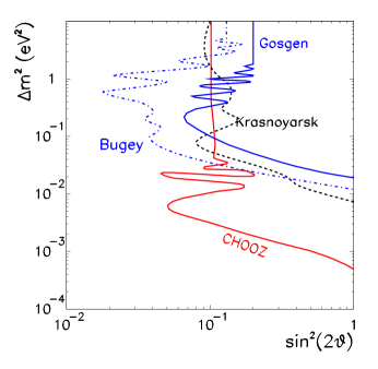
Figure 4: Excluded regions at 90% for $\nu_{e}$ oscillations from searches in reactors experiments at short baselines.

Smaller values of $\Delta m^{2}$ can be accessed in a reactor experiment using a longer baseline. Pursuing this idea, the KamLAND experiment [85], a 1000 ton liquid scintillation detector, is currently in operation in the Kamioka mine in Japan. This underground site is located at an average distance of 150-210 km from several Japanese nuclear power stations. The measurement of the flux and energy spectrum of the $\bar{\nu}_{e}$’s emitted by these reactors provides a test of neutrino oscillations with $\Delta m^{2}\gtrsim 10^{-5}~{}\text{eV}^{2}$.

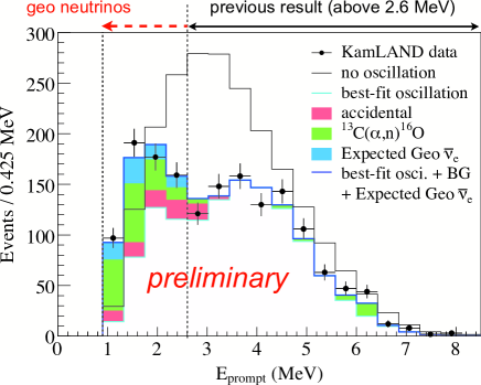
Figure 5: Prompt event energy spectrum of $\bar{\nu}_{e}$ events at KamLAND from Ref. [86].

In their first result corresponding to an exposure of 162 ton-yr (145.1 days), the ratio of the number of observed inverse $\beta$-decay events to the number of events expected without oscillations is $R_{\text{KamLAND}}~{}=0.611\pm 0.094$ for $E_{\bar{\nu}_{e}}>$ 3.4 MeV [87]. This deficit is inconsistent with the expected rate for massless $\bar{\nu}_{e}$’s at the 99.95% confidence level. In June 2004 KamLAND also presented the energy dependence of their events in the form of the prompt energy ($E_{\text{prompt}}\simeq E_{\bar{\nu}_{e}}+m_{p}-m_{n}$) spectrum [88]. Finally, in September 2007 the collaboration released a new analysis with increased statistics and a lower energy threshold [86]. In Fig. 5 we show their observed spectrum (from Ref. [86]) which clearly shows that the deficit is energy dependent as expected from neutrino oscillations.

2.4 Accelerator Neutrinos at Long Baselines

Conventional neutrino beams from accelerators are mostly produced by $\pi$ decays (and some $K$ decays), with the pions produced by the scattering of the accelerated protons on a fixed target:

$$\begin{array}[]{lll}p+\text{target}\to&\lx@intercol\pi^{\pm}+X\hfil\lx@intercol\\ &\pi^{\pm}\to&\mu^{\pm}+\nu_{\mu}(\bar{\nu}_{\mu})\\ &&\mu^{\pm}\to e^{\pm}+\nu_{e}(\bar{\nu}_{e})+\bar{\nu}_{\mu}(\nu_{\mu})\end{array}$$ (90)

Thus the beam can contain both $\mu$- and $e$-neutrinos and antineutrinos. The final composition and energy spectrum of the neutrino beam is determined by selecting the sign of the decaying $\pi$ and by stopping the produced $\mu$ in the beam line. There is an additional contribution to the electron neutrino and antineutrino flux from kaon decay.

Indeed the accelerator neutrino beams are very similar in nature to the atmospheric neutrinos and they can be used to test the observed oscillation signal with a controlled beam. Given the characteristic $\Delta m^{2}$ involved in the interpretation of the atmospheric neutrino signal, the intense neutrino beam from the accelerator must be aimed at a detector located underground at a distance of several hundred kilometers.

The first of these long baseline experiments with accelerator beams has been K2K [89] which run with a baseline of about 235 km from KEK to SK. MINOS [90] is currently running with a baseline of 730 km from Fermilab, where the near detector is placed, to the Soudan mine where the far detector is located.

The results from both K2K and MINOS [91, 92, 93], both in the observed deficit of events and in their energy dependence confirm that accelerator $\nu_{\mu}$ oscillate over distances of several hundred kilometers as expected from oscillations with the parameters compatible with those inferred from the atmospheric neutrino data.

In their last analysis K2K reported the observation of 107 fully contained events while the expectation in the absence of oscillations is $151^{+12}_{-10}$. In the left panel of Fig. 6 we show their latest data on the observed energy spectrum compared with the expectations in the absence of oscillations as well as the best fit in the presence of oscillations (from Ref. [92]).

The complete 5.4 kton MINOS far detector has been taking data since the beginning of August 2003 and in March 2006 presented their first results on the comparison of the rate and energy spectra of the charged current neutrino interactions between the two detectors based on a luminosity of $1.27\times 10^{20}$ protons on target. They observed a total of 122 events below 10 GeV while the expectation without oscillations is $238.7\pm 10.7$. In the right panel of Fig. 6 we show their published data on the observed energy spectrum compared with the expectations in the absence of oscillations as well as their best fit in the presence of oscillations (from Ref. [93]). In summer 2007 MINOS presented an updated analysis based on a total integrated luminosity of $\sim$ $2.5\times 10^{20}$ protons on target [94]. In their preliminary analysis they report a slightly lower value of $\Delta m^{2}=2.38^{+0.20}_{-0.16}~{}\text{eV}^{2}$ than in their previously published result.

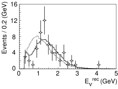
Figure 6: (Left) The reconstructed $E_{\nu}$ distribution of the 1-ring $\mu$-like sample in K2K (from Ref. [92]). The dashed line is the expected spectrum without oscillation normalized to the observed number of events. The solid line is the best fit spectrum in presence of oscillations with $\Delta m^{2}=2.8\times 10^{-3}~{}\text{eV}^{2}$ and $\sin^{2}2\theta=1$. (Right) Reconstructed energy spectra of the observed CC events in MINOS (from Ref. [93]). and comparison with the unoscillated and oscillated spectrum for $\Delta m^{2}=2.74\times 10^{-3}~{}\text{eV}^{2}$ and $\sin^{2}2\theta=1$.

The OPERA [95, 96] neutrino detector at the underground Gran Sasso Laboratory (LNGS) was designed to perform the first detection of neutrino oscillations in appearance mode, through the observation of $\nu_{\tau}$ appearance. It is placed in the high-energy, long-baseline CERN to LNGS beam (CNGS) 730 km away from the neutrino source. In August 2006 a first run with CNGS neutrinos was successfully conducted. A first sample of neutrino events was collected, statistically consistent with the integrated beam intensity [97].

2.5 Accelerator Neutrinos at Short Baselines

Most oscillation experiments performed with neutrino beams from accelerators have characteristic distances of the order of hundreds of meters. We call them short baseline (SBL) experiments. With the exception of the LSND experiment, which we discuss below, all searches have been negative. In Table 3 we show the limits on the various transition probabilities from the negative results of the most restricting SBL experiments. Due to the short path length, these experiments are not sensitive to the low values of $\Delta m^{2}$ which we find when trying to explain either the solar or the atmospheric neutrino data.

Table 3: 90% CL limit on the neutrino oscillation probabilities from the negative searches at short baseline experiments.

Experiment	Beam	Channel	Limit (90%)	$\Delta m^{2}_{\text{min}}$ ($\text{eV}^{2}$)	Ref.
CDHSW	CERN	$\nu_{\mu}\rightarrow\nu_{\mu}$	$P_{\mu\mu}>0.95$	00.250	[98]
E776	BNL	$\nu_{\mu}\rightarrow\nu_{e}$	$P_{e\mu}<1.5\times 10^{-3}$	00.075	[99]
E734	BNL	$\nu_{\mu}\rightarrow\nu_{e}$	$P_{e\mu}<1.6\times 10^{-3}$	00.400	[100]
KARMEN2	Rutherford	$\bar{\nu}_{\mu}\rightarrow\bar{\nu}_{e}$	$P_{e\mu}<6.5\times 10^{-4}$	00.050	[101]
E531	FNAL	$\nu_{\mu}\rightarrow\nu_{\tau}$	$P_{\mu\tau}<2.5\times 10^{-3}$	00.900	[102]
CCFR/	FNAL	$\nu_{\mu}\rightarrow\nu_{e}$	$P_{\mu e}<8\times 10^{-4}$	01.600	[103, 104]
NUTEV		$\bar{\nu}_{\mu}\rightarrow\bar{\nu}_{e}$	$P_{\mu e}<5.5\times 10^{-4}$	02.400	[104]
		$\nu_{\mu}\rightarrow\nu_{\tau}$	$P_{\mu\tau}<4\times 10^{-3}$	01.600	[105]
		$\nu_{e}\rightarrow\nu_{\tau}$	$P_{e\tau}<0.1$	20.000	[106]
Chorus	CERN	$\nu_{\mu}\rightarrow\nu_{\tau}$	$P_{\mu\tau}<3.4\times 10^{-4}$	00.600	[107]
		$\nu_{e}\rightarrow\nu_{\tau}$	$P_{e\tau}<2.6\times 10^{-2}$	07.500	[107]
Nomad	CERN	$\nu_{\mu}\rightarrow\nu_{\tau}$	$P_{\mu\tau}<1.7\times 10^{-4}$	00.700	[108]
		$\nu_{e}\rightarrow\nu_{\tau}$	$P_{e\tau}<7.5\times 10^{-3}$	05.900	[108]
		$\nu_{\mu}\rightarrow\nu_{e}$	$P_{\mu e}<6\times 10^{-4}$	00.400	[108]

The only positive signature of oscillations at a short baseline laboratory experiment comes from the Liquid Scintillator Neutrino Detector (LSND) [109] running at Los Alamos Meson Physics Facility. Its primary neutrino flux came from $\pi^{+}$’s produced in a 30-cm-long water target when hit by protons from the LAMPF linac with 800 MeV kinetic energy. The detector was a tank filled with 167 metric tons of dilute liquid scintillator, located about 30 m from the neutrino source. The experiment observed an excess of events as compared to the expected background while the excess was consistent with $\bar{\nu}_{\mu}\to\bar{\nu}_{e}$ oscillations. In the latest results the total fitted excess was of $87.9\pm 22.4\pm 6$ events, corresponding to an oscillation probability of $(2.64\pm 0.67\pm 0.45)\times 10^{-3}$. For oscillations between two neutrino states these results lead to the oscillation parameters shown in Fig. 7. The shaded regions are the 90% and 99% likelihood regions from LSND.

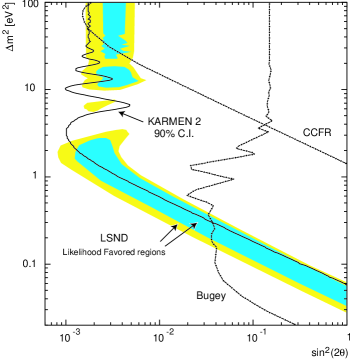
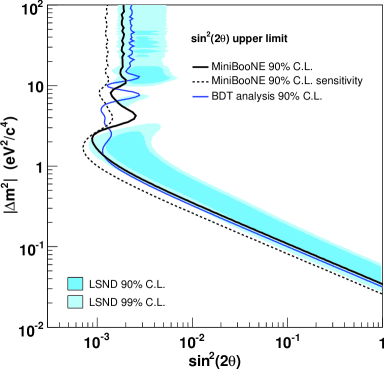
Figure 7: (Left) Allowed regions (at 90% and 99% CL) for $\nu_{e}\to\nu_{\mu}$ oscillations from the LSND experiment compared with the exclusion regions (at 90% CL) from KARMEN2 and other experiments (from Ref. [101]). (Right) $\nu_{\mu}\rightarrow\nu_{e}$ excluded regions from MiniBooNE compared to the LSND allowed region (from Ref. [110]).

The region of parameter space which is favored by the LSND observations has been partly tested by other experiments like the KARMEN [101] experiment and very recently by MiniBooNE [110].

The KARMEN experiment was performed at the neutron spallation facility ISIS of the Rutherford Appleton Laboratory. They found a number of events in good agreement with the total background expectation. The corresponding exclusion curve from the final data set recorded with the full experimental set up of KARMEN2 in the two-neutrino parameter space is given in Fig. 7 together with the favored region for the LSND experiment. At large $\Delta m^{2}$, KARMEN2 results exclude the region favored by LSND. At low $\Delta m^{2}$, KARMEN2 leaves some allowed space, but the reactor experiments at Bugey and CHOOZ add stringent limits for the larger mixing angles.

In Ref. [111] a combined statistical analysis of the experimental results of the LSND and KARMEN search was performed. At a combined confidence level of 36 %, they found no area of oscillation parameters compatible with both experiments. For the complementary confidence of $1-0.36=64$ %, they found two well defined regions of oscillation parameters with either $\Delta m^{2}\approx 7~{}\text{eV}^{2}$ or $\Delta m^{2}<1~{}\text{eV}^{2}$ compatible with both experiments.

2.5.1 MiniBooNE

The MiniBooNE experiment [112], currently running at Fermilab, searches for $\nu_{\mu}\to\nu_{e}$ oscillations and was specially designed to make a conclusive statement about the LSND’s neutrino oscillation evidence. In their 2002-2005 run they used a $\nu_{\mu}$ beam of energy $0.5-1.0$ GeV initiated by a primary beam of 8.89 GeV protons from the Fermilab Booster impinging on a 71 cm long and 1 cm diameter beryllium target. The target is located inside a magnet focusing horn. The beam contains only a small intrinsic $\nu_{e}$ component. In January 2006, MiniBooNE switched the polarity of the horn to select negative sign mesons and since then the experiment has been collecting data using a beam of antineutrinos.

The MiniBooNE detector is a 12.2 m diameter sphere filled with 800 tons of pure mineral oil. The center of the detector is positioned at a distance of 541 m from the front of the Beryllium target. The vessel consists of two optically isolated regions separated by a support structure. The inner region of 5.5 m radius is the neutrino target region, while the outer volume forms the veto region.

Figure 8: Reconstructed $E_{\nu}$ of the observed $\nu_{e}$ events recorded by MiniBooNE compared with the expected background and the expectations in the presence of oscillations with oscillation parameters characteristic of the LSND signal (from Ref. [110]).

In their analysis of the neutrino data released on April 2007 [110] they studied the events with reconstructed neutrino energy $300<E_{\nu}<3000$ MeV. Their observed spectrum of $\nu_{e}$ events is shown in Fig. 8. As seen in the figure the spectrum presents and excess of $96\pm 17\pm 20$ events for $E_{\nu}<475$ MeV while there is no significant excess of events for $E_{\nu}>475$ ($22\pm 19\pm 35$ events above expectation). In Ref. [110] MiniBooNE claims that the low-energy excess cannot be explained by a $2\nu$-oscillation model and consequently the collaboration performed their oscillation analysis using only the events with $E_{\nu}>475$ MeV. With this data they find a $\chi^{2}$ probability of 93% for the null oscillation hypothesis and at 90% CL their single-sided roster scan excluded region shows no overlap with the 90% allowed region of the LSND evidence for $2\nu$ oscillations as seen in the right panel of Fig. 7 (from Ref. [110]). In Ref. [110] they also performed a joint analysis of LSND and MiniBooNE which excludes the $2\nu$ oscillation hypothesis as an explanation of the LSND anomaly at 98% CL.

3 3-$\nu$ Mixing

3.1 Dominant 2-$\nu$ Oscillations for Solar Neutrinos and KamLAND

The simplest explanation of the solar neutrino data described in Sec. 2.1 is the oscillations of $\nu_{e}$ into an active ($\nu_{\mu}$ and/or $\nu_{\tau}$) or a sterile ($\nu_{s}$) neutrino. Oscillations into pure sterile neutrinos are strongly disfavored by the SNO data because if the beam comprises of only $\nu_{e}$’s and $\nu_{s}$’s, the three observed CC, ES and NC fluxes should be equal (up to effects due to spectral distortions), an hypothesis which is now ruled out at more than $7\sigma$ by the SNO data (see Eq. (86)).

The goal of the analysis of the solar neutrino data in terms of neutrino oscillations is to determine which range of mass-squared difference and mixing angle can be responsible for the observed deficit. In order to answer this question in a statistically meaningful way one must compare the predictions in the different oscillation regimes with the observations, including all the sources of uncertainties and their correlations. In the present analysis the main sources of uncertainty are the theoretical errors in the prediction of the solar neutrino fluxes for the different reactions. These errors are due to uncertainties in the twelve basic ingredients of the solar model, which include the nuclear reaction rates (parametrized in terms of the astrophysical factors $S_{11}$, $S_{33}$, $S_{34}$, $S_{1,14}$ and $S_{17}$), the solar luminosity, the metallicity $Z/X$, the Sun age, the opacity, the diffusion, and the electronic capture of ${}^{7}\text{Be}$, $C_{\text{Be}}$. Another source of theoretical error arises from the uncertainties in the neutrino interaction cross section for the different detection processes. A detailed description of the way to include all these uncertainties and correlations can be found in Ref. [3] and references therein.

As illustration we show in Fig. 9 the results of the analysis of the total event rates as it was in the summer of 2001 including the total rates from Chlorine, Gallium, SK and the first determination of the CC event rates at SNO. In the figure we plot the allowed regions which correspond to 90%, 95%, 99% and 99.73% ($3\sigma$) CL for $\nu_{e}$ oscillations into active neutrinos (2 d.o.f.). As seen in the figure, there were several oscillation regimes compatible within errors with the experimental data. These allowed parameter regions are denoted as MSW small mixing angle (SMA), MSW large mixing angle (LMA), MSW low mass (LOW) and vacuum oscillations (VAC).

For the LMA solution, oscillations for the ${}^{8}\text{B}$ neutrinos occur in the adiabatic regime and the survival probability is higher for lower energy neutrinos. This situation fits well the higher rate observed at gallium experiments. For the LOW solution, the situation is opposite but matter effects in the Earth for pp and ${}^{7}\text{Be}$ neutrinos enhance the average annual survival probability for these lower energy neutrinos. The combination of these effects still allows a reasonable description of the Gallium rate. For the SMA solution the oscillations for the ${}^{8}\text{B}$ neutrinos occur in the non-adiabatic regime while for the VAC solution the oscillation wavelength is of the order of the Sun-Earth distance for ${}^{8}\text{B}$ neutrinos.

Further information on the different oscillation regimes can be obtained from the analysis of the energy and time dependence data from SK and SNO. For example, for LMA and LOW, the expected energy spectrum at these experiments is very little distorted. Also in the lower part of the LMA region and in the upper part of the LOW region matter effects in the Earth are important and some day-night variation is expected. For SMA, a positive slope of the energy spectrum is predicted, with larger slope for larger mixing angle within SMA. For VAC, large distortions of the energy spectrum are expected as imprints of the $L/E$ dependence of the survival probability. The quantification of these effects depends on the precise values of the oscillation parameters.

The observed day-night spectrum in SK and SNO are essentially undistorted in comparison to the SSM expectation and shows no significant differences between the day and the night periods as commented in Sec. 2.1. Consequently, a large region of the oscillation parameter space where these variations are expected to be large can be excluded. In particular:

• SMA: within this region, the part with larger mixing angle fails to comply with the observed energy spectrum, while the part with smaller mixing angles gives a not good enough fit to the total rates.

• VAC: the observed undistorted energy spectrum cannot be accommodated.

• LMA and LOW: the small $\Delta m^{2}$ part of LMA and the LOW solution are eliminated because they predict a day-night variation that is larger than observed.

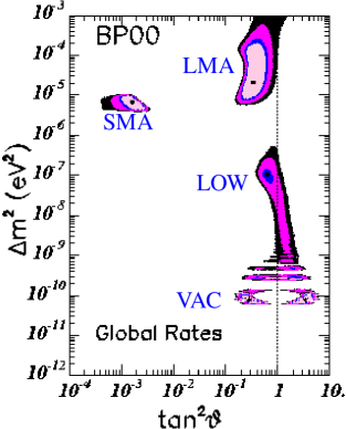
Figure 9: Allowed oscillation parameters (at 90%, 95%, 99% and 99.73% CL) from the analysis of the total event rates of the Chlorine, Gallium, SK and the first SNO CC experiments (adapted from Ref. [113]).

Thus with the inclusion of the time and energy dependence of the ${}^{8}\text{B}$ neutrino fluxes at SK and SNO it was possible to select the LMA as the most favored solution to the solar neutrino problem. We show in Fig. 10 the allowed region of parameters which correspond to 90%, 95%, 99% and 99.73% ($3\sigma$) CL for $\nu_{e}$ oscillations from the global analysis of the latest solar neutrino data. The Borexino results are in perfect agreement with the expectations within the LMA region, but they are not included in the analysis because they are still not precise enough to have an impact on the determination of the oscillation parameters.

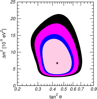
Figure 10: Allowed oscillation parameters (at 90%, 95%, 99% and 99.73% CL) from the global analysis of the solar neutrino data.

As mentioned in Sec. 2 these small values of $\Delta m^{2}$ could also be accessed the terrestrial experiment KamLAND using as beam the $\bar{\nu}_{e}$’s from nuclear reactors located over distances of the order of hundred kilometers. Indeed the KamLAND results can be interpreted in terms of $\bar{\nu}_{e}$ oscillations with parameters shown in Fig. 11.

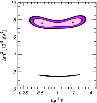
Figure 11: Allowed oscillation parameters (at 90%, 95%, 99% and 99.73% CL) from the analysis of KamLAND data. Based on calculations by T. Schwetz.

The most important aspect of Fig. 11 is the demonstration by KamLAND that anti-neutrinos oscillate with parameters that are consistent with the LMA solution of the solar neutrino problem. Under the assumption that CPT is satisfied, the anti-neutrino measurements by KamLAND apply directly to the neutrino sector and the two sets of data can be combined to obtain the globally allowed oscillation parameters. The results of such an analysis are shown in Fig. 12.

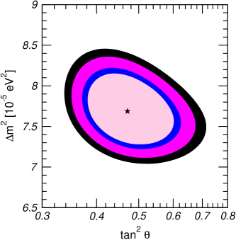
Figure 12: Allowed oscillation parameters (at 90%, 95%, 99% and 99.73% CL) from the combined analysis of solar and KamLAND data.

3.2 Dominant 2-$\nu$ Oscillations for Atmospheric and LBL Neutrinos

The simplest and most direct interpretation of the atmospheric neutrino data described in Sec. 2.2 is that of muon neutrino oscillations. The required value of the oscillation parameters can be easily estimated from the following observations:

• The angular distribution of contained events shows that, for $E\sim 1$ GeV, the deficit comes mainly from $L\sim 10^{2}-10^{4}$ km. The corresponding oscillation phase must be maximal, $\frac{\Delta m^{2}(\text{eV}^{2})L(\text{km})}{2E(\text{GeV})}\sim 1$, which requires $\Delta m^{2}\sim 10^{-4}-10^{-2}~{}\text{eV}^{2}$.

• Assuming that all upgoing $\nu_{\mu}$’s which would lead to multi-GeV events oscillate into a different flavor while none of the downgoing ones do, the up-down asymmetry is given by $|A_{\mu}|=\sin^{2}2\theta/(4-\sin^{2}2\theta)$. The present one sigma bound reads $|A_{\mu}|>0.27$ which requires that the mixing angle is close to maximal, $\sin^{2}2\theta>0.85$.

In order to go beyond these rough estimates, one must compare in a statistically meaningful way the experimental data with the theoretical expectations. The most up-to-date details on our determination of the expected rates in SK-I and SK-II and the corresponding statistical analysis can be found in Appendix A.

Altogether the best interpretation of the atmospheric neutrino data is the oscillation of $\nu_{\mu}$ into $\nu_{\tau}$. In Fig. 13 we plot the allowed regions from the global analysis of atmospheric data.

Other oscillation channels are presently ruled out. $\nu_{\mu}\to\nu_{e}$ is excluded with high CL as the explanation to the atmospheric neutrino anomaly for two different reasons:

• SK high precision data show that the $\nu_{e}$ contained events are very well described by the SM prediction both in normalization and in their zenith angular dependence;

• Explaining the atmospheric data with $\nu_{\mu}\to\nu_{e}$ transition has direct implications for the $\bar{\nu}_{e}\to\bar{\nu}_{\mu}$ transition. In particular, there should be a $\bar{\nu}_{e}$ deficit in the CHOOZ reactor experiment which was not observed.

$\nu_{\mu}\rightarrow\nu_{s}$ is also ruled out as a possible explanation of the atmospheric neutrino anomaly because the presence of matter effects in this channel predict a flatter-than-observed angular distribution of thru-upgoing muon events [114]. Also if $\nu_{\mu}$ oscillates into sterile neutrinos one expects a relative suppression of the NC signal which has not been observed [115]. Furthermore recently Super-Kamiokande has performed a dedicated analysis for the search for the effects of appearance of tau neutrinos which disfavors the hypothesis of no $\nu_{\tau}$ appearance at $2.4\sigma$ [116].

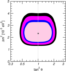
Figure 13: Allowed regions from the analysis of atmospheric neutrino data. The different contours correspond to at 90%, 95%, 99% and $3\sigma$ CL.

As we have described in Sec. 2.4, the results of the LBL experiments K2K and MINOS confirm, both in the observed deficit of events and in their energy dependence, that accelerator $\nu_{\mu}$ oscillate over distances of several hundred kilometers as expected from oscillations with the parameters previously inferred from the atmospheric neutrino data. This is quantitatively illustrated in Fig. 14 where we show the results of our analysis of the K2K and MINOS data respectively. As seen in the figure, both K2K and MINOS provide an independent determination of the relevant $\Delta m^{2}$ and, in particular, they favor the upper part of the atmospheric mass-splitting while they have very limited sensitivity to the mixing angle which is still dominantly determined by the atmospheric neutrino data.

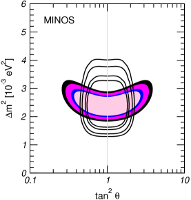
Figure 14: Allowed regions from the analysis of K2K (left) and MINOS (right) (full regions). For K2K only the 90%, 95% and and 99% CL regions are shown. For comparison we also show the corresponding allowed regions from ATM neutrinos at the same CL (lines).

3.3 Subdominant 3-$\nu$ Oscillation Effects

From the results previously described it is obvious that the minimum joint description of solar and atmospheric evidences requires that all three known neutrinos take part in the oscillations. In this case, the mixing parameters are encoded in the $3\times 3$ lepton mixing matrix [29, 33] which can be conveniently parametrized in the standard form of Eq. (39), since the two Majorana phases in Eq. (38) do not affect neutrino oscillations [117, 118].

The determination of the oscillation probabilities for both solar and atmospheric neutrinos requires that one solves the evolution equation of the neutrino system, Eq. (70), in the matter background of the Sun and the Earth. In the three-flavor framework, the equation in the flavor basis can be written as:

$$i\frac{d\vec{\nu}}{dx}=H\,\vec{\nu},\qquad H=U\cdot H_{0}^{d}\cdot U^{\dagger}+V\,,$$ (91)

where $U$ is the lepton mixing matrix, $\vec{\nu}\equiv(\nu_{e},\,\nu_{\mu},\,\nu_{\tau})^{T}$ and

$$H_{0}^{d}=H_{m}-\frac{m_{1}}{2E}=\frac{1}{2E}\mathop{\mathrm{diag}}\left(0,\,\Delta m^{2}_{21},\,\Delta m^{2}_{31}\right)\,.$$ (92)

$V$ is the effective potential that describes CC forward interactions in matter, Eq. (64).

In total the three-neutrino oscillation analysis involves six parameters: two mass differences (including two possible signs for one of them), three mixing angles and one CP phase.

Without loss of generality one can chose the mass differences as shown in Fig. 15 so that $\Delta m^{2}_{21}$ is always positive and there are two possible mass orderings which we denote as normal and inverted and which correspond to the two possible choices of the sign of $\Delta m^{2}_{31}$. In this convention the angles $\theta_{ij}$ can be taken without loss of generality to lie in the first quadrant, $\theta_{ij}\in[0,\pi/2]$ and the phases $\delta_{\text{CP}},\;\eta_{i}\in[0,2\pi]$.

The normal ordering is naturally related to hierarchical masses, $m_{1}\ll m_{2}\ll m_{3}$, for which $m_{2}\simeq\sqrt{\Delta m^{2}_{21}}$ and $m_{3}\simeq\sqrt{\Delta m^{2}_{32}}$, or to quasi-degenerate masses, $m_{1}\simeq m_{2}\simeq m_{3}\gg\Delta m^{2}_{21},\Delta m^{2}_{32}$. On the other hand, the inverted ordering implies that $m_{3}<m_{1}\simeq m_{2}$.

With this assignment (see more below) $\Delta m^{2}_{21}$ and the mixing angle $\theta_{12}$ have been chosen to be those that give the dominant oscillations for solar neutrinos while $\Delta m^{2}_{31}$, $\Delta m^{2}_{32}$ and $\theta_{23}$ give the dominant oscillation for atmospheric neutrinos.

Figure 15: Mass schemes for $3\nu$ oscillations

Generic three-neutrino oscillation effects are:

• Mixing effects because of the additional angle $\theta_{13}$

• Difference between Normal and Inverted schemes,

• Coupled oscillations with two different oscillation lengths,

• CP violating effects.

The strength of these effects is controlled by the values of the ratio of mass differences, the mixing angle $\theta_{13}$ and the CP phase $\delta_{\text{CP}}$.

In this respect, as we have seen in the previous sections, the parameter space of solutions for solar and atmospheric oscillations in Figs. 13 and 12 satisfy

$$\Delta m^{2}_{21}=\Delta m^{2}_{\odot}\ll\Delta m^{2}_{\text{atm}}=|\Delta m^{2}_{31}|\simeq|\Delta m^{2}_{32}|.$$ (93)

This hierarchy implies that even though in general the transition probabilities present an oscillatory behavior with two oscillation lengths, in present experiments, such interference effects are not very visible.

In this notation, the survival probability of reactor antineutrinos at CHOOZ takes the form:

$$\begin{split}P_{ee}^{\text{CHOOZ}}&=1-\cos^{4}\theta_{13}\sin^{2}2\theta_{12}\sin^{2}\left(\frac{\Delta m^{2}_{21}L}{4E}\right)\\ &\hskip 5.69054pt-\sin^{2}2\theta_{13}\left[\cos^{2}\theta_{12}\sin^{2}\left(\frac{\Delta m^{2}_{31}L}{4E}\right)+\sin^{2}\theta_{12}\sin^{2}\left(\frac{\Delta m^{2}_{32}L}{4E}\right)\right]\\ &\simeq 1-\sin^{2}2\theta_{13}\sin^{2}\left(\frac{\Delta m^{2}_{31}L}{4E}\right)\,,\end{split}$$ (94)

where we have used that for the relevant values of energy and distance, one can safely neglect Earth matter effects. The second equality holds under the approximation $\Delta m^{2}_{21}\ll E/L$ which can be safely made for $\Delta m^{2}_{21}\leq 3\times 10^{-4}~{}\text{eV}^{2}$ Thus effectively the analysis of the CHOOZ reactor data involves two oscillation parameters the mass difference which drives the dominant atmospheric and K2K oscillations, $\Delta m^{2}_{31}$, and the angle $\theta_{13}$ which is severely constrained [119].

3.3.1 Effects due to $\theta_{13}$ in Solar Neutrinos and KamLAND

Let us first consider the analysis of solar and KamLAND neutrinos. A first simplification occurs because $L^{\text{osc}}_{31}=4\pi E/\Delta m^{2}_{31}$ is much shorter than the distance between the Sun and the Earth for solar neutrinos or between the reactors and the detectors in KamLAND. Consequently, the oscillations related to ${L_{0,31}^{\text{osc}}}$ are averaged and the vacuum survival probability can be obtained from Eq. (44) with $\sin^{2}X_{31}=\sin^{2}X_{32}=1/2$. It is trivial to show that it can be written in the following form:

$$P^{3\nu}_{ee}=\sin^{4}\theta_{13}+\cos^{4}\theta_{13}P^{2\nu}_{ee}(\Delta m^{2}_{21},\theta_{12})\,,$$ (95)

For solar neutrinos one must also take into account the three-neutrino mixing effects in the evolution in matter. In this case a second simplification occurs since, for the evolution in both the Sun and the Earth, $\Delta m^{2}_{31}\gg 2\sqrt{2}G_{F}n_{e}E\sin^{2}2\theta_{13}$. Consequently, matter effects on the evolution of $\nu_{3}$ can be neglected. The net result is that for solar neutrinos the survival probability can also be written as Eq. (95) with $P^{2\nu}_{ee}$ obtained taking into account evolution in the effective density [120, 121]:

$$n_{e}\Rightarrow n_{e}\cos^{2}\theta_{13}\,.$$ (96)

We conclude that the analysis of the solar and KamLAND data constrains three of the six independent oscillation parameters: $\Delta m^{2}_{21},\theta_{12}$ and $\theta_{13}$.

Eq. (95) reveals what is the dominant effect of a non-vanishing $\theta_{13}$ in the solar and KamLAND neutrino survival probability: the survival probability, $P^{2\nu}_{ee}$, gets reduced by the factor $\cos^{4}\theta_{13}$, while an energy independent term, $\sin^{4}\theta_{13}$, is added. Within the present allowed values of $\theta_{13}$ the first effect is the most relevant.

3.3.2 Effects due to $\theta_{13}$ in Atmospheric and LBL Neutrinos

We discuss first the sub-leading effect due to the mixing angle $\theta_{13}$ which is particularly easy to treat in the hierarchical approximation in which $\Delta m^{2}_{21}$-induced oscillations are neglected in the atmospheric neutrino analysis. In this approximation one can rotate away the angle $\theta_{12}$. Thus the resulting survival probabilities do not depend on $\Delta m^{2}_{21}$ and $\theta_{12}$. For instance for constant Earth matter density, the various $P_{\alpha\beta}$ can be written as follows:

$$P_{ee} =1-4s^{2}_{13,m}c^{2}_{13,m}\,S_{31}\,,$$ (97)

$$P_{\mu\mu} =1-4s^{2}_{13,m}c^{2}_{13,m}s^{4}_{23}\,S_{31}-4s^{2}_{13,m}s^{2}_{23}c^{2}_{23}\,S_{21}-4c^{2}_{13,m}s^{2}_{23}c^{2}_{23}\,S_{32}\,,$$ (98)

$$P_{e\mu} =4s^{2}_{13,m}c^{2}_{13,m}s^{2}_{23}\,S_{31}\,,$$ (99)

Here $\theta^{m}_{13}$ is the effective mixing angle in matter:

$$\sin 2\theta^{m}_{13}=\frac{\sin 2\theta_{13}}{\sqrt{(\cos 2\theta_{13}-2EV_{e}/\Delta m^{2}_{31})^{2}+(\sin 2\theta_{13})^{2}}}$$ (100)

and $S_{ij}$ are the oscillating factors in matter:

$$S_{ij}=\sin^{2}\left(\frac{\Delta\mu^{2}_{ij}}{4E}L\right).$$ (101)

In Eq. (101), $\Delta\mu^{2}_{ij}$ are the effective mass-squared differences in matter:

$$\Delta\mu^{2}_{21} =\frac{\Delta m^{2}_{31}}{2}\left(\frac{\sin 2\theta_{13}}{\sin 2\theta^{m}_{13}}-1\right)-EV_{e}\,,$$ (102)

$$\Delta\mu^{2}_{32} =\frac{\Delta m^{2}_{31}}{2}\left(\frac{\sin 2\theta_{13}}{\sin 2\theta^{m}_{13}}+1\right)+EV_{e}\,,$$ (103)

$$\Delta\mu^{2}_{31} =\Delta m^{2}_{31}\frac{\sin 2\theta_{13}}{\sin 2\theta^{m}_{13}}\,.$$ (104)

and $L$ is the path length of the neutrino within the Earth.

The main effect of $\theta_{13}$ is that now atmospheric neutrinos can oscillate simultaneously in both the $\nu_{\mu}\to\nu_{\tau}$ and $\nu_{\mu}\to\nu_{e}$ (and, similarly, $\nu_{e}\to\nu_{\tau}$ and $\nu_{e}\to\nu_{\mu}$) channels. The oscillation amplitudes for channels involving $\nu_{e}$ are controlled by the size of $\sin^{2}\theta_{13}=|U_{e3}|^{2}$. Furthermore because of matter effects the size of the effect is different for normal and inverted hierarchies [122, 123, 124, 125, 126, 127, 128, 129, 130].

In Fig. 16 we show the expected zenith angular distribution of contained e-like events (normalized to the no-oscillation expectation) for $\sin^{2}\theta_{13}=0.04$. From the figure we see that the effect is most relevant for multi-GeV neutrinos and larger for the normal-hierarchy than inverted orderings. Also the effect can be a decrease or increase of the expected number of events with respect to the $\theta_{13}=0$ prediction depending on whether $\theta_{23}$ is in the first or second octant. These results can be understood as follows. From Eqs. (97)–(99) it is easy to show that for the case of constant matter density the expected flux of $\nu_{e}$ events in the hierarchical approximation can be written as [124, 125]:

$$\frac{N_{e}}{N_{e0}}-1=\langle P_{e\mu}\rangle\,\bar{r}(s_{23}^{2}-\frac{1}{\bar{r}})\,,$$ (105)

where $\langle P_{e\mu}\rangle$ is the corresponding probability, Eq. (99), averaged over energy and zenith angle, and $\bar{r}=\Phi_{\mu 0}/\Phi_{e0}$ is the ratio of the electron and muon neutrino fluxes in the absence of oscillations in the relevant energy and angular bin.

For instance, for sub-GeV events $\bar{r}\sim 2$. So the effect cancels for maximal $\theta_{23}$. For $\theta_{23}$ in the first octant ($s_{23}^{2}<0.5$) there is a decrease in the number of electron events as compared to the $\theta_{13}$ case while the opposite holds for $\theta_{23}$ in the second octant. Thus the effect is suppressed for maximal $\theta_{23}$ mixing.

For multi-GeV events matter effects lead to an enhancement of the effect which is slightly larger for the normal ordering where the matter enhancement is in the neutrino channel. For sub-GeV events, the matter term can be neglected and the effect of a non-vanishing $\theta_{13}$ is smaller and it is the same for normal and inverted ordering.

For K2K and MINOS, matter effects can be neglected and the relevant survival probability takes the form

$$\begin{split}P^{\text{K2K, MINOS}}_{\mu\mu}&=1-4\left(s^{4}_{23}s^{2}_{13}c^{2}_{13}+c^{2}_{13}s^{2}_{23}c^{2}_{23}\right)\sin^{2}\left(\frac{\Delta m^{2}_{31}}{4E}L\right)\\ &\simeq s_{13}^{2}\frac{\cos 2\theta_{23}}{c_{23}^{2}}+\left(1-s_{13}^{2}\frac{\cos 2\theta_{23}}{c_{23}^{2}}\right)P^{\text{K2K,$2\nu$}}_{\mu\mu}(\Delta m^{2}_{31},\theta_{23})+\mathcal{O}(s_{13}^{4})\,.\end{split}$$ (106)

So we find that in the approximation of Eq. (93) the analysis of the atmospheric and K2K+MINOS data constrains three of the six independent oscillation parameters: $\Delta m^{2}_{31}$, $\theta_{23}$ and $\theta_{13}$ and for atmospheric neutrinos also the sign of $\Delta m^{2}_{31}$ is relevant. Consequently in this approximation the mixing angle $\theta_{13}$ is the only parameter common to both solar+KamLAND and atmospheric+K2K neutrino oscillations and which may potentially allow for some mutual influence.

3.3.3 Effects due to $\Delta m^{2}_{21}$ in Atmospheric Neutrinos

We next discuss the sub-leading effects due to $\Delta m^{2}_{21}$ oscillations for vanishing small value of $\theta_{13}$ [131, 132, 133, 134, 135, 136, 137, 138, 139]. In this approximation and for constant Earth matter density the relevant oscillation probabilities can be written as:

$$P_{ee} =1-P_{e2}\,,$$ (107)

$$P_{e\mu} =c_{23}^{2}P_{e2}\,,$$ (108)

$$P_{\mu\mu} =1-c_{23}^{4}P_{e2}-2s_{23}^{2}c_{23}^{2}\,\left[1-\sqrt{1-P_{e2}\cos\phi}\right]\,,$$ (109)

where

$$P_{e2}=\sin^{2}2\theta_{12,m}\sin^{2}\left(\frac{\Delta m^{2}_{21}\,L}{4E}\frac{\sin 2\theta_{12}}{\sin 2\theta_{12,m}}\right)\,,$$ (110)

with

$$\sin 2\theta_{12,m} =\dfrac{\sin 2\theta_{12}}{\sqrt{\left(\cos 2\theta_{12}\mp\dfrac{2EV_{e}}{\Delta m^{2}_{21}}\right)^{2}+\sin^{2}2\theta_{12}}}\,,$$ (111)

$$\phi \approx(\Delta m^{2}_{31}+s_{12}^{2}\,\Delta m_{21}^{2})\frac{L}{2E}\,.$$ (112)

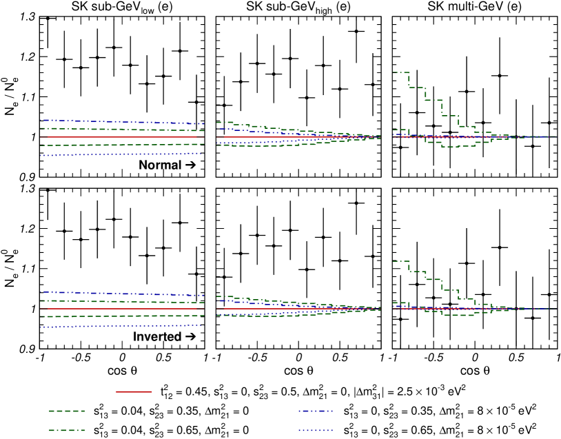
Figure 16: Comparison of the sub-leading effects due to $\Delta m^{2}_{21}$- and $\theta_{13}$-induced $\nu_{e}$ oscillations in the expected zenith angular distribution of e-like events.

In Fig. 16 we show the angular distribution of atmospheric $\nu_{e}$ for non-vanishing values of $\Delta m^{2}_{21}$ or $\theta_{13}$. As seen in these figures, unlike for $\theta_{13}$, the main effect of a small but non-vanishing $\Delta m^{2}_{21}$ is mostly observable for sub-GeV electrons, and it can result either in an increase or in a decrease of the expected number of events with respect to the $\Delta m^{2}_{21}=0$ prediction depending on whether $\theta_{23}$ is in the first or second octant. This behavior can be understood in terms of the approximate analytical expressions:

$$\frac{N_{e}}{N_{e0}}-1 =\langle P_{e2}\rangle\,\bar{r}\left(c_{23}^{2}-\frac{1}{\bar{r}}\right)$$ (113)

$$\frac{N_{\mu}-N_{\mu}(\Delta m^{2}_{21}=0)}{N_{\mu 0}} =-\langle P_{e2}\rangle\,c_{23}^{2}\left(c_{23}^{2}-\frac{1}{\bar{r}}\right)$$ (114)

where $N_{e0}$ and $N_{\mu 0}$ are the expected number of electron and muon-like events in the absence of oscillations in the relevant energy and angular bin and $N_{\mu}(\Delta m^{2}_{21}=0)$ is the expected number of muon-like events for $\Delta m^{2}_{21}=0$. For sub-GeV events, $\Delta m^{2}\ll 2EV_{e}$ so

$$P_{e2}=\sin^{2}2\theta_{12}\left(\frac{\Delta m^{2}_{21}}{2EV_{e}}\right)^{2}\sin^{2}\frac{V_{e}L}{2}\,.$$ (115)

According to Eqs. (113) and (114) the sign of the shift in the number of predicted events is opposite for electron and muon-like events and it depends on the factor $c_{23}^{2}-\frac{1}{\bar{r}}\sim c_{23}^{2}-0.5$. So the effect cancels for maximal $\theta_{23}$. For $\theta_{23}$ in the first octant, $c_{23}^{2}>0.5$, there is an increase (decrease) in the number of electron (muon) events as compared to the $\Delta m^{2}_{21}=0$ case. For $\theta_{23}$ in the second octant the opposite holds ( this is the opposite behavior than the one due to $\theta_{13}\neq 0$ previously discussed). We also see that the net shift is larger for electron events than for muon events by a factor $c_{23}^{2}/\bar{r}$. In summary for sub-GeV electrons, the shift in the expected number of events is proportional to the deviation of $\theta_{23}$ from maximal mixing and to $(\Delta m^{2}_{21})^{2}$, it is very weakly dependent on the zenith angle, and it decreases with the energy.

The present data may already give some hint of deviation of the 2-3 mixing from maximal as seen in Fig. 3. Indeed as the figure illustrates, there is some excess of the $e-$like events in the sub-GeV range. The excess increases with decrease of energy within the sample as expected from a $\Delta m^{2}_{21}$ effect.

3.3.4 Interference of $\theta_{13}$ and $\Delta m^{2}_{21}$ effects

Figure 17: Sub-leading effect due to the interference of $\Delta m^{2}_{21}$- and $\theta_{13}$-induced $\nu_{e}$ oscillations in the expected zenith angular distribution of e-like events.

Finally we comment on the possible effects due to the interference between $\theta_{13}$- and $\Delta m^{2}_{21}$-induced oscillations [138, 140, 141] which could give sensitivity to the CP violating phase $\delta_{\text{CP}}$. This effect is most important for sub-GeV energies for which one can write [141]:

$$\frac{N_{e}}{N_{e}^{0}}-1\simeq\langle P_{e2}\rangle\,\bar{r}\left(c_{23}^{2}-\frac{1}{\bar{r}}\right)+2\tilde{s}_{13}^{2}\,\bar{r}\left(s_{23}^{2}-\frac{1}{\bar{r}}\right)\\ -\bar{r}\tilde{s}_{13}\tilde{c}_{13}^{2}\sin 2\theta_{23}\left(\cos\delta_{\text{CP}}\langle R_{2}\rangle-\sin\delta_{\text{CP}}\langle I_{2}\rangle\right)$$ (116)

where

$$P_{e2} =\sin^{2}2\theta_{12,m}\,\sin^{2}\frac{\phi_{m}}{2}\,,$$ (117)

$$R_{2} =-\sin 2\theta_{12,m}\cos 2\theta_{12,m}\,\sin^{2}\frac{\phi_{m}}{2}\,,$$ (118)

$$I_{2} =-\frac{1}{2}\sin 2\theta_{12,m}\,\sin\phi_{m}\,,$$ (119)

$$\tilde{\theta}_{13} \approx\theta_{13}\left(1+\frac{2E\,V_{e}}{\Delta m^{2}_{31}}\right)\,.$$ (120)

Here $\phi_{m}$ is the phase oscillation in matter and $\theta_{12,m}$ is 12 the mixing angle in matter (Eq. (111)). As seen from Eq. (116) the interference term (third term in the equation) is not suppressed for maximal $\theta_{23}$ so it can dominate for $\theta_{23}$ near maximal. Also it is proportional to $\sin 2\theta_{23}$ and therefore it is not sensitive to the octant of $\theta_{23}$. Fig. 17 illustrates the possible size of this effect.

3.4 Global $3\nu$ Analysis of Oscillation Data

The results of the global combined analysis including all dominant and subdominant oscillation effects are summarized in Fig. 18 and Fig. 19 in which we show different projections of the allowed 6-dimensional parameter space. New to previous analysis is the inclusion of the latest MINOS and of the SK-II atmospheric data and the inclusion in the analysis of the effect of $\delta_{\text{CP}}$.

In Fig. 18 we plot the correlated bounds from the global analysis several pairs of parameters. The regions in each panel are obtained after marginalization of $\chi^{2}_{\text{global}}$ with respect to the three undisplayed parameters. The different contours correspond to regions defined at 90%, 95%, 99% and $3\sigma$ CL for 2 d.o.f. ($\Delta\chi^{2}=4.61$, $5.99$, $9.21$, $11.83$) respectively. From the figure we see that the stronger correlation appears between $\theta_{13}$ and $\Delta m^{2}_{31}$ as a reflection of the CHOOZ bound. In the lower panels we show the allowed regions in the ($\sin^{2}\theta_{13}$, $\delta_{\text{CP}}$) plane. As seen in the figure, the sensitivity to the CP phase at present is marginal but we find that the present bound on $\sin^{2}\theta_{13}$ can vary by about $\sim$ 30% depending on the exact value of $\delta_{\text{CP}}$. This arises from the interference of $\theta_{13}$ and $\Delta m^{2}_{21}$ effects in the atmospheric neutrino observables as described above. To illustrate this point we plot in the same panel the bounds on $\sin^{2}\theta_{13}$ at 90%, 95%, 99% and $3\sigma$ CL if the atmospheric data is not included in the analysis (the vertical lines).

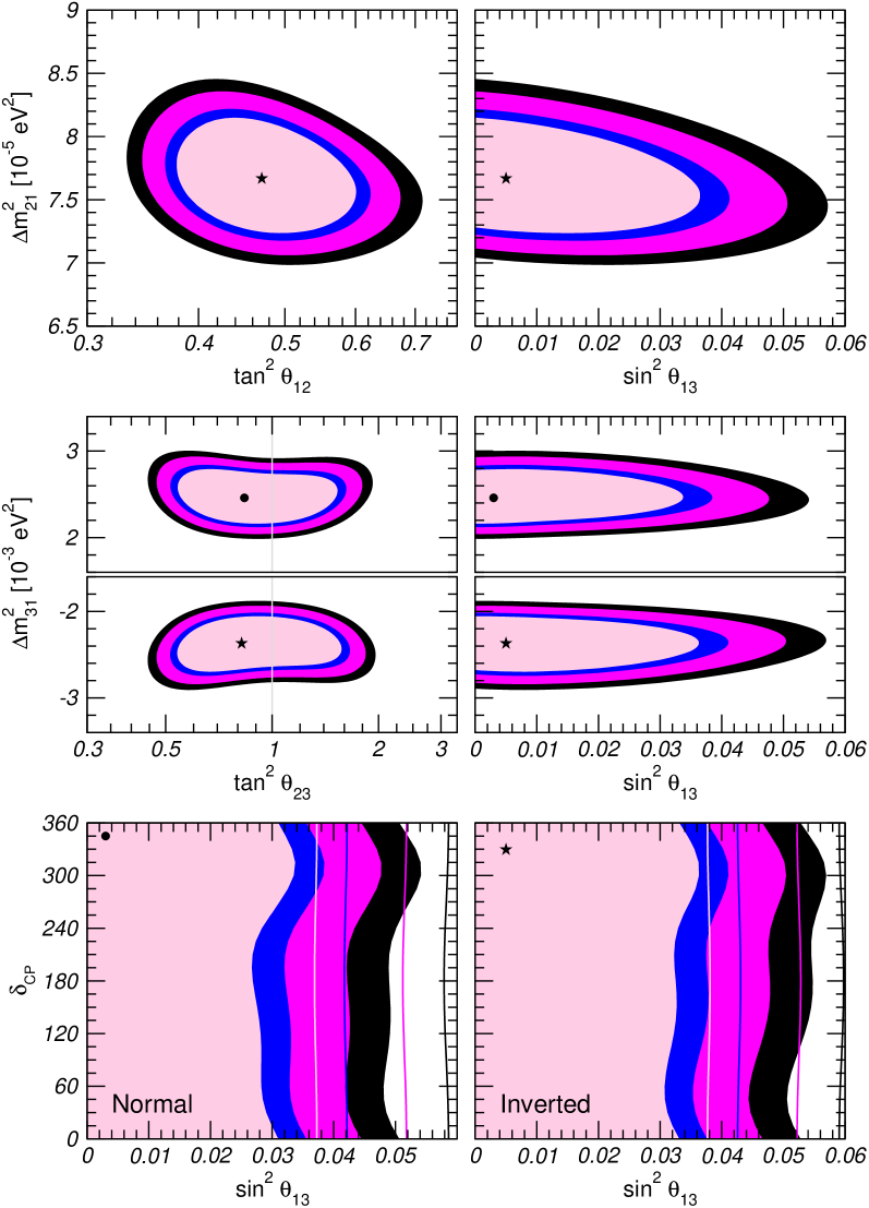
Figure 18: Global $3\nu$ oscillation analysis. Each panels shows 2-dimensional projection of the allowed 5-dimensional region after marginalization with respect to the undisplayed parameters. The different contours correspond to the two-dimensional allowed regions at 90%, 95%, 99% and $3\sigma$ CL. In the lowest panel the vertical lines correspond to the regions without inclusion of the atmospheric neutrino data.

In Fig. 19 we plot the individual bounds on each of the six relevant parameters derived from the global analysis (full line). To illustrate the impact of the LBL and KamLAND data we also show the corresponding bounds when KamLAND and the LBL data are not included in the analysis respectively. In each panel, except the lower left one, the displayed $\chi^{2}$ has been marginalized with respect to the other five parameters. The lower left panel shows the $\chi^{2}$ (marginalized over all parameters but $\theta_{13}$) dependence of $\delta_{\text{CP}}$ for fixed values of $\theta_{13}$.

Figure 19: Global $3\nu$ oscillation analysis. Each panels shows the dependence of $\Delta\chi^{2}$ on each of the parameters from the global analysis (full line) compared to the bound prior to the KamLAND data (dashed lines in the first row) and LBL data (dashed lines in the second rows). In the lowest panel we show the dependence of $\Delta\chi^{2}$ on $\theta_{13}$ for different sets of data as labeled in the curves. The individual $1\sigma$ ($3\sigma$) bounds in Eqs. (121) can be read from the corresponding panel with the condition $\Delta\chi^{2}\leq 1$ ($9$).

The derived ranges for the six parameters at $1\sigma$ ($3\sigma$) are:

$$\Delta m^{2}_{21} =7.67\,_{-0.21}^{+0.22}\,\left({}_{-0.61}^{+0.67}\right)\times 10^{-5}~{}\text{eV}^{2}\,,$$ (121)

$$\Delta m^{2}_{31} =\begin{cases}-2.37\pm 0.15\,\left({}_{-0.46}^{+0.43}\right)\times 10^{-3}~{}\text{eV}^{2}&\text{(inverted hierarchy)}\,,\\[2.84526pt] +2.46\pm 0.15\,\left({}_{-0.42}^{+0.47}\right)\times 10^{-3}~{}\text{eV}^{2}&\text{(normal hierarchy)}\,,\end{cases}$$

$$\theta_{12} =34.5\pm 1.4\,\left({}_{-4.0}^{+4.8}\right)\,,$$

$$\theta_{23} =42.3\,_{-3.3}^{+5.1}\,\left({}_{\hphantom{0}-7.7}^{+11.3}\right)\,,$$

$$\theta_{13} =0.0\,^{+7.9}_{-0.0}\,\left({}^{+12.9}_{\hphantom{0}-0.0}\right)\,,$$

$$\delta_{\text{CP}} \in[0,\,360]\,.$$

Figure 19 illustrates that the dominant effect of the inclusion of the laboratory experiments KamLAND, K2K and MINOS is the better determination of the corresponding mass differences $\Delta m^{2}_{21}$ and $\Delta m^{2}_{31}$ while the mixing angle $\theta_{12}$ is dominantly determined by the solar data and the mixing angle $\theta_{23}$ is still most precisely measured in the atmospheric neutrino experiments. The non-maximality of the best $\theta_{23}$ observed in Eq. (121) is a pure 3-$\nu$ oscillation effect associated to the inclusion of the $\Delta m^{2}_{21}$ effects in the atmospheric neutrino analysis. As discussed above, although statistically not very significant, this preference for non-maximal 2-3 mixing is a physical effect on the present neutrino data, induced by the fact than an excess of events is observed in sub-GeV electrons but not in sub-GeV muons nor, in the same amount, in the multi-GeV electrons. As a consequence, this excess cannot be fully explained by a combination of a global rescaling and a “tilt” of the fluxes within the assumed uncertainties.

Finally, let’s notice that the ranges in Eq. (121) are not independent but they are correlated so they cannot be directly used to determine the leptonic mixing matrix at a given CL. As described in Ref. [142] the leptonic mixing matrix can be consistently extracted as follows. Starting by the $\chi^{2}_{\text{global}}$ which is a function of the six parameters, we can define the mass-marginalized $\chi^{2}$ function:

$$\chi^{2}_{\text{mix,global}}(\theta_{12},\theta_{23},\theta_{13},\delta_{\text{CP}})=\\ \text{min}_{(\Delta m^{2}_{21},\Delta m^{2}_{31})}\,\chi^{2}_{\text{global}}(\Delta m^{2}_{21},\Delta m^{2}_{31},\theta_{12},\theta_{23},\theta_{13},\delta_{\text{CP}})\,.$$ (122)

We study the variation of $\chi^{2}_{\text{mix,global}}$ as function of each of the mixing combinations in $U$ as follows. For a given magnitude $\bar{U}_{ij}$ of the entry $U(i,j)$ we define $\chi^{2}(\bar{U}_{ij})$ as the minimum value of $\chi^{2}_{\text{mix, global}}$ with the condition $|U(i,j)(\theta_{12},\theta_{23},\theta_{13},\delta_{\text{CP}})|=\bar{U}_{ij}$. The allowed range of the magnitude of the entry $ij$ at a given CL is then defined as the values $\bar{U}_{ij}$ verifying

$$\chi^{2}(\bar{U}_{ij})-\chi^{2}_{\text{global,min}}\leq\Delta\chi^{2}(\text{CL, 1~{}d.o.f.})\,.$$ (123)

With this procedure we derive the following values on the magnitude of the elements of the complete matrix, at 90% CL:

$$|U|_{\text{90\%}}=\begin{pmatrix}0.80\to 0.84&~{}\quad~{}0.53\to 0.60&~{}\quad~{}0.00\to 0.17\\ 0.29\to 0.52&~{}\quad~{}0.51\to 0.69&~{}\quad~{}0.61\to 0.76\\ 0.26\to 0.50&~{}\quad~{}0.46\to 0.66&~{}\quad~{}0.64\to 0.79\end{pmatrix}$$ (124)

and at the $3\sigma$ level:

$$|U|_{3\sigma}=\begin{pmatrix}0.77\to 0.86&~{}\quad~{}0.50\to 0.63&~{}\quad~{}0.00\to 0.22\\ 0.22\to 0.56&~{}\quad~{}0.44\to 0.73&~{}\quad~{}0.57\to 0.80\\ 0.21\to 0.55&~{}\quad~{}0.40\to 0.71&~{}\quad~{}0.59\to 0.82\end{pmatrix}\,.$$ (125)

By construction these limits are obtained under the assumption that $U$ is unitary. In other words, the ranges in the different entries of the matrix are correlated due to the fact that, in general, the result of a given experiment restricts a combination of several entries of the matrix, as well as to the constraints imposed by unitarity. As a consequence choosing a specific value for one element further restricts the range of the others. Effects in the determination of the leptonic mixing matrix due to violations of unitarity have been considered in Ref. [143].

4 Learning about Solar and Atmospheric Neutrino Fluxes

4.1 Motivation

As we have described in previous sections the flavor oscillation hypothesis has been supported by an impressive wealth of neutrino experimental data. Originally, the two most important pieces of evidence came from solar and atmospheric neutrino experiments.

The expected number of solar and atmospheric neutrino events in an experiment depends on a variety of components: the neutrino fluxes, the neutrino oscillation parameters and the neutrino interaction cross section in the detector. Although the original goal of the experiments was the understanding of the solar and atmospheric neutrino fluxes, once it was found that the observed anomalies seemed to indicate that neutrinos oscillated, the main focus of the experiments changed to the determination of the neutrino masses and mixing. Consequently, in the standard analysis, such as the ones described in Sec. 3, the remaining components of the event rate computation are inputs taken from other sources. In particular, as discussed in Sec. 2.1, the fluxes of solar neutrinos are taken from the results of Solar Model simulations [45] which describe the properties of the Sun and its evolution based on a set of observational parameters and basic assumptions such as spherical symmetry, thermal equilibrium, etc…. Similarly, the fluxes of atmospheric neutrinos are taken from the results of numerical calculations, such as those of Refs. [66, 65, 67, 68, 69], which are based on the convolution of the primary cosmic ray spectrum with the expected yield of neutrinos per incident cosmic ray.

The oscillation of $\nu_{e}$ and $\nu_{\mu}$’s can also be tested at terrestrial facilities. In particular, the disappearance of reactor antineutrinos can be used to detect $\bar{\nu}_{e}$ oscillations as described in Sec. 2.3, and $\nu_{\mu}$ oscillations can be studied in Long Baseline experiments (see Sec. 2.4) using as neutrino source a controlled beam of accelerator neutrinos. As we have seen, the results of KamLAND [88], K2K [92] and MINOS [93] have confirmed both in the observed deficit of events and in their energy dependence, that reactor $\bar{\nu}_{e}$ and accelerator $\nu_{\mu}$ oscillate as expected from oscillations with the parameters inferred from the solar and atmospheric neutrino data respectively. Furthermore they already provide a competitive independent determination of the relevant $\Delta m^{2}$.

The attainable accuracy in the independent determination of the relevant neutrino oscillation parameters from non-solar and non-atmospheric neutrino experiments makes it possible to attempt an inversion of the strategy: to use the oscillation parameters (independently determined in reactor and LBL neutrino experiments) as inputs in the solar and atmospheric neutrino analysis in order to extract the solar and atmospheric neutrino fluxes directly from the data. Alternatively one can perform global fits to natural (solar and atmospheric) and terrestrial (reactor and accelerator) neutrino data in which both the oscillation parameters and the natural fluxes are extracted simultaneously.

There are several motivations for such direct determination of the solar and atmospheric neutrino fluxes. First of all it would provide a cross-check of the standard flux calculations as well as of the size of the associated uncertainties (which, being mostly theoretical, are difficult to quantify). Also, such program quantitatively expands the physics potential of future solar and atmospheric neutrino experiments.

4.2 Learning How the Sun Shines

The idea that the Sun generates power through nuclear fusion in its core was first suggested in 1919 by Sir Arthur Eddington, who pointed out that the nuclear energy stored in the Sun could explain the apparent age of the Solar System.

In 1939, Hans Bethe described in an epochal paper [144] two nuclear fusion mechanisms by which main sequence stars like the Sun could produce the energy corresponding to their observed luminosities. The two mechanisms have become known as the $pp$ chain and the CNO cycle [16]. For both the $pp$ chain and the CNO cycle the basic energy source is the burning of four protons to form an alpha particle,two positrons, and two neutrinos. In the $pp$ chain, fusion reactions among elements lighter than $A=8$ produce a characteristic set of neutrino fluxes, whose spectral energy shapes are known but whose fluxes must be calculated with a detailed solar model. In the CNO chain, with ${}^{12}\text{C}$ as a catalyst, ${}^{13}\text{N}$ and ${}^{15}\text{O}$ beta decays are the primary source of neutrinos.

The first sentence in Bethe’s paper reads: “It is shown that the most important source of energy in ordinary stars is the reactions of carbon and nitrogen with protons.” Bethe’s conclusion about the dominant role of the CNO cycle relied upon a crude model of the Sun. Over the next two and a half decades, the results of increasingly more accurate laboratory measurements of nuclear fusion reactions and more detailed solar model calculations led to the theoretical inference that the Sun shines primarily by the $pp$ chain rather than the CNO cycle. Currently, solar model calculations imply [45] that 98.5% of the solar luminosity is provided by the $pp$ chain and only 1.5% is provided by CNO reactions.

Despite the obvious appeal of the theory, simple observations of the solar luminosity are not enough to demonstrate that nuclear fusion is, in fact, the solar energy source neither the role of the CNO versus the $pp$ chain in the energy generation. Only neutrinos, with their extremely small interaction cross sections, can enable us to see into the interior of a star and thus verify directly the hypothesis of nuclear energy generation in stars [145].

Indeed from the earliest days of solar neutrino research, a primary goal of the field was to test the energy generation model of the Sun and in particular the solar model prediction that the Sun shines by the $pp$ chain and not by the CNO cycle [146, 147]. However this task was made difficult by the fact that neutrino oscillations occur and they change in an energy dependent way the probability that electron type neutrinos created in the Sun reach the Earth as electron type neutrinos. This affects both the overall number of events in the solar neutrino experiments and the relative contribution expected from the different components of the solar neutrino spectrum. Because of these complications, the extraction of the fluxes from the solar neutrino data was not possible, and, for example, one could find neutrino oscillation solutions in which 99.95% of the Sun’s luminosity is supplied by the CNO cycle [148].

As a consequence until very recently, it was necessary to assume the standard solar model predictions for all the solar neutrino fluxes and their uncertainties in order to determine reasonably constrained values for neutrino oscillation parameters. Only the upcome of the real time experiments Super-Kamiokande and SNO and the independent determination of the oscillation parameters using reactor antineutrinos at KamLAND allowed for the attempt to extract the solar neutrino fluxes and their uncertainties directly from the data [149, 150, 151, 152, 153] as we describe next.

4.2.1 Solar Neutrino Fluxes from Neutrino Data

There are eight thermonuclear reactions which can produce neutrinos in the Sun. Neutrino fluxes are named by the corresponding source reaction. Five reactions produce $\nu_{e}$ in the $pp$ chain ($pp$, $pep$, $hep$, ${}^{7}\text{Be}$, and ${}^{8}\text{B}$) and three in the CNO cycle (${}^{13}\text{N}$, ${}^{15}\text{O}$, and ${}^{17}\text{F}$). Most of these reactions produce a neutrino spectrum characteristic of $\beta$ decay while in some cases, like the ${}^{7}\text{Be}$ neutrinos, the spectrum is almost monochromatic, with an energy width of about 2 keV which is characteristic of the temperature in the core of the Sun. In general, the physics which determines the neutrino energy spectrum in each of the reactions is well understood. Thus in the extraction of the solar neutrino fluxes from the neutrino data one assumes that the energy dependence of the fluxes is well determined by nuclear physics and only the rates of the different reactions is to be tested. Under this assumption, the empirical determination of the solar fluxes reduces to extracting from the data the value of the eight normalization constants giving the rate of each of the contributions. For convenience these are usually parametrized in terms of some factors $f_{i}$ giving the ratios of the “true” solar neutrino fluxes and the fluxes predicted by some solar model:

$$f_{i}\equiv\frac{\phi_{i}}{\phi_{i}^{\text{SSM}}}\,,$$ (126)

with $i=pp$, $pep$, $hep$, ${}^{7}\text{Be}$, ${}^{8}\text{B}$, ${}^{13}\text{N}$, ${}^{15}\text{O}$, ${}^{17}\text{F}$.

The most directly determined flux is the ${}^{8}\text{B}$ flux because both Super-Kamiokande and SNO detect the interaction of ${}^{8}\text{B}$ neutrinos. Under the hypothesis of no sterile neutrino mixing this flux is exactly given by the NC rate observed at SNO

$$f_{B}=\frac{R^{\text{NC,exp}}_{\text{SNO}}}{R^{\text{NC,SSM}}_{\text{SNO}}}=0.87\pm 0.08\,.$$ (127)

where $R^{\text{SSM}}_{\text{SNO}}$ is the NC rate for the SNO experiment that is predicted by the standard solar model in the absence of oscillations:

$$R^{\text{NC,SSM}}_{\text{SNO}}=\int\phi^{\text{SSM}}(^{8}\text{B},E_{\nu})\,\sigma^{NC}(E_{\nu})\,R^{\text{SSM}}_{\text{SNO}}\,dE_{\nu}\,.$$ (128)

$E_{\nu}$ is the neutrino energy and $\sigma^{NC}$ is the weighted average $\nu_{e}$-d NC interaction cross-section, including the experimental energy resolution function.

Independently of the presence of sterile neutrinos the ${}^{8}\text{B}$ flux can be extracted from the CC rate at SNO [149] once the oscillation parameters have been independently determined, for example, at KamLAND:

$$f_{\text{B}}=\frac{R^{\text{CC,exp}}_{\text{CC,SNO}}}{R^{\text{SSM}}_{\text{SNO}}}\times\frac{1}{\langle P_{ee}(\Delta m^{2},\theta)\rangle_{\text{SNO}}},$$ (129)

where ${\langle P_{ee}(\Delta m^{2},\tan^{2}\theta)\rangle_{\text{SNO}}}$ is the average survival probability for electron-flavor neutrinos detected at SNO in the CC interactions for a given value of the oscillation parameters:

$$\langle P_{ee}(\Delta m^{2},\theta)\rangle_{\text{SNO}}=\frac{1}{R^{\text{CC,SSM}}_{\text{SNO}}}\int\phi^{\text{SSM}}(^{8}\text{B},E_{\nu})\,\sigma^{CC}(E_{\nu})\,P_{ee}(E_{\nu},\Delta m^{2},\theta)\,dE_{\nu}\,.$$ (130)

Similarly the lower energy fluxes can be extracted from the radiochemical experiments. For example, the expected event rate in the gallium experiments is a sum of the contributions from the different neutrino fluxes:

$$R_{\text{Ga}}=f_{\text{B}}\,R^{{}^{8}\text{B},\text{SSM}}_{\text{Ga}}\langle P_{ee}(\Delta m^{2},\theta)\rangle^{{}^{8}\text{B}}_{\text{Ga}}\,\\[5.69054pt] +f_{\text{Be}}\,R^{{}^{7}\text{Be},\text{SSM}}_{\text{Ga}}\langle P_{ee}(\Delta m^{2},\theta)\rangle^{{}^{7}\text{Be}}_{\text{Ga}}+\sum_{i}f_{i}\,R^{\phi_{i},SSM}_{\text{Ga}}\langle P_{ee}(\Delta m^{2},\theta)\rangle^{\phi_{i}}_{\text{Ga}}\,.$$ (131)

where the average survival probabilities are obtained similarly to Eq. (130) with the corresponding fluxes and cross sections. The last term in Eq. (131) contains the contributions from $hep$, $pep$, CNO and $pp$ neutrinos. Substituting the value of $f_{\text{B}}$ determined from the KamLAND and SNO CC measurements, Eq. (129), into Eq. (131), one can solve Eq. (131) for $f_{\text{Be}}$ by equating $R_{\text{Ga}}=R^{\text{exp}}_{\text{Ga}}$. In order to do so one has to to assume that all the solar neutrino fluxes but the ${}^{8}\text{B}$ and ${}^{7}\text{Be}$ fluxes are equal to the values predicted by the SSM.

Alternatively, instead of trying to determine one flux at a time, one can perform a global fit to all solar and reactor neutrino data in which both the oscillation parameters and the flux normalization constants $f_{i}$ are determined. A key ingredient in these type of analysis is the imposition of the luminosity constraint [154]. The luminosity constraint implements, in a global way for the Sun, the constraint of conservation of energy for nuclear fusion among light elements. Each neutrino flux is associated with a specific amount of energy released to the star and therefore a particular linear combination of the solar neutrino fluxes is equal to the solar luminosity (in appropriate units). One can write the luminosity constraint as

$$\frac{L_{\odot}}{4\pi\text{(A.U.)}^{2}}=\sum\limits_{i}\alpha_{i}\phi_{i}\,,$$ (132)

where $L_{\odot}$ is the solar luminosity measured at the Earth’s surface, 1 $A.U.$ is the average Earth-Sun distance, and the coefficient $\alpha_{i}$ is the amount of energy provided to the star by nuclear fusion reactions associated with each of the important solar neutrino fluxes, $\phi_{i}$. The coefficients $\alpha_{i}$ are calculated accurately in Ref. [154]. An additional simplification comes from the fact that the ratio of the $pep$ neutrino flux to the $pp$ neutrino flux is fixed to high accuracy because they have the same nuclear matrix element.

At present, this strategy yields the following value for the flux normalization constants

$$f_{pp}=f_{pep} =1.0\pm 0.02$$ (133)

$$f_{{}^{8}\text{B}} =0.88\pm 0.04$$

$$f_{{}^{7}\text{Be}} =1.03^{+0.24}_{-1.03}$$

$$f_{{}^{13}\text{N}} =0.0^{+7.6}_{-0.0}$$

$$f_{{}^{15}\text{O}} =0.0^{+5.0}_{-0.0}$$

$$f_{{}^{17}\text{F}} =0.0^{+2.1}_{-0.0}$$

at 1$\sigma$. Concerning the very small $hep$ flux, the global fit has very little sensitivity to this flux. At present the best determination of this flux is an upper bound, $f_{hep}\lesssim 5$, which has been derived from the search of events with $E_{\nu}>16$ MeV at the SNO experiment [155].

From the results in Eq. (133) it is possible, for example, to extract the allowed range of the fraction of the Sun’s luminosity that arises from CNO reactions as [150, 151]:

$$\frac{L_{CNO}}{L_{\odot}}=\sum\limits_{i=\text{N,O,F}}\left(\frac{\alpha_{i}}{10~{}\text{MeV}}\right)a_{i}\,f_{i}\,,$$ (134)

where $a_{i}$ is the ratio of the neutrino flux $i$ predicted by the standard solar model to the characteristic solar photon flux defined by $L_{\odot}/[4\pi\text{(A.U.)}^{2}(\text{10 MeV})]$. At present this determination gives a bound

$$\frac{L_{\text{CNO}}}{L_{\odot}}=0.0^{+2.7}_{-0.0}\,(^{+7.3}_{-0.0})\,\%$$ (135)

at $1\sigma$ ($3\sigma$). So the global fit to all the data yields a constraint which is consistent with the solar model prediction at $1\sigma$ which is an important empirical confirmation of the SSM and, in general, of our understanding of the Sun.

As mentioned above a very important ingredient on the determination of the solar fluxes given in Eq. (133) is the imposition of the luminosity constraint. For example, it is this constraint that implies that the $pp$ flux is known with a precision, $\pm 2\%$, comparable to the theoretical uncertainty, $\pm 1\%$ in the SSM prediction. On the contrary if one does not impose the luminosity constraint on the extraction of the solar neutrino fluxes one finds that both the $pp$ and ${}^{7}\text{Be}$ fluxes as well as the CNO luminosity fraction are very poorly known.

Alternatively one may try to test the luminosity constraint itself, by comparing the inferred luminosity based on the neutrino fluxes extracted from the fit without imposing that condition, with the observed photon luminosity. Such a test can tell us whether there are any energy generation mechanisms beyond nuclear fusion. In addition, we can learn whether the Sun is in a steady state, because the neutrino luminosity tells us how it burns today, while the photons tell us how it burned over 40,000 years ago. With the existing data, however, the experimental precision is not enough to allow for such a test. In other words the current comparison of these luminosities is not very precise [152]. Quantitatively we obtain that the inferred luminosity based on the neutrino fluxes is:

$$\frac{L_{\odot}\text{(neutrino-inferred)}}{L_{\odot}}=1.4^{+0.2}_{-0.3}\,(^{+0.7}_{-0.6})\,.$$ (136)

We see that, at $3\sigma$, the inferred luminosity can be 2.1 times larger than the measured photon luminosity, or 0.8 times smaller. The fact that the solar neutrino flux is overwhelmingly $pp$ neutrinos means that the precision of this comparison approximately scales with the precision of a measurement of the $pp$ flux. Therefore a future low energy solar neutrino experiment has the potential to perform such a fit as we describe in Sec. 7.1.

4.3 General Strategy for Atmospheric Flux Determination

The determination of atmospheric neutrino fluxes directly from the atmospheric neutrino data is technically more involved than for solar neutrinos because there are four different fluxes to be determined: $\nu_{e}$, $\nu_{\mu}$, $\bar{\nu}_{e}$, and $\bar{\nu}_{\mu}$ which, after integration over the azimuthal angle, are a function of two variables: the zenith angle and the energy of the neutrino. Unlike for solar neutrinos, there is no simple physics which can determine the angular and energy dependence of the fluxes thus not only the normalization of the fluxes but also their functional dependence has to be extracted from the data. Consequently the fully empirically determination of the atmospheric fluxes from atmospheric neutrino data requires a generic parametrization of the energy and angular functional dependence of the fluxes which is valid in all the range of energies where there is available data. Such parametrization does not exist.

The problem of the unknown functional form for the neutrino flux can be bypassed by the use of neural networks as interpolants. Artificial neural networks have long been used in different fields, from biology to high energy physics, and from pattern recognition to business intelligence applications. In this context artificial neural networks allow the parametrization of the atmospheric neutrino flux without having to assume any functional behavior. Indeed, the problem of the deconvolution of the atmospheric flux from experimental data on event rates is rather close in spirit to the determination of parton distribution functions in deep-inelastic scattering from experimentally measured structure functions [156]. Consequently a similar strategy can be applied to determine the atmospheric fluxes. This approached was followed in Ref. [157] and can be summarized as follows:

• In the first stage, a Monte Carlo sample of replicas of the experimental data on neutrino event rates (“artificial data”) is generated. These can be viewed as a sampling of the probability measure on the space of physical observables at the discrete points where data exist.

• In the second stage one uses neural networks to interpolate between these points. In order to do so one has to first determine the atmospheric event rates for a given atmospheric flux, and second to compare these rates to the data in order to tune the best-fit form of input neural flux distribution. This process is called the “training of the neural network”.

Combining these two steps, the space of physical observables is mapped onto the space of fluxes, so the experimental information on the former can be interpolated by neural networks in the latter.

We describe briefly now how this procedure can be applied to the data from Super-Kamiokande. The starting point, of course, is the observed event rates:

$$R_{i}^{\text{(exp)}},\qquad i=1,\ldots,N_{\text{dat}}\,,$$ (137)

which contain information on the value of the atmospheric fluxes in the range of 0.1 GeV $\lesssim E_{\nu}\lesssim$ few TeV and on their flavor and angular dependence.

For this data the experimental correlation matrix can be constructed as:

$$\rho^{\text{(exp)}}_{ij}=\frac{(\sigma^{\text{stat}}_{i})^{2}\delta_{ij}+\displaystyle\sum_{n=1}^{N_{\text{cor}}}\sigma^{\text{cor}}_{ni}\,\sigma^{\text{cor}}_{nj}}{\sigma^{\text{tot}}_{i}\,\sigma^{\text{tot}}_{j}}\,,$$ (138)

where the statistical uncertainty is given by

$$\sigma^{\text{stat}}_{i}=\sqrt{R_{i}^{\text{(exp)}}}\,.$$ (139)

The $N_{\text{cor}}$ correlated uncertainties are computed from the couplings factors, $\pi_{i}^{n}$ to the corresponding pull $\xi_{n}$ [158] (see Appendix A):

$$\sigma^{\text{cor}}_{ni}\equiv R_{i}^{\text{(exp)}}\pi_{i}^{n}\,,$$ (140)

and the total error is computed adding the statistical and correlated errors in quadrature.

The purpose of the artificial data generation is to produce a Monte Carlo set of ‘pseudo–data’, i.e. $N_{\text{rep}}$ replicas of the original set of $N_{\text{dat}}$ data points:

$$R^{(\text{art})(k)}_{i}\,,\qquad k=1,\dots,N_{\text{rep}}\,,\qquad i=1,\dots,N_{\text{dat}}\,,$$ (141)

such that the $N_{\text{rep}}$ sets of $N_{\text{dat}}$ points are distributed according to an $N_{\text{dat}}$–dimensional multi-gaussian distribution around the original points, with expectation values equal to the central experimental values, and error and covariance equal to the corresponding experimental quantities.

This is achieved by defining

$$R_{i}^{(\text{art})(k)}=R_{i}^{\text{(exp)}}+r_{i}^{(k)}\sigma_{i}^{\text{tot}},\qquad i=1,\ldots,N_{\text{dat}}\,,\qquad k=1,\ldots,N_{\text{rep}}\,,$$ (142)

where $N_{\text{rep}}$ is the number of generated replicas of the experimental data, and where $r_{i}^{(k)}$ are univariate gaussian random numbers with the same correlation matrix as experimental data, that is they satisfy

$$\langle r_{i}^{(k)}r_{j}^{(k)}\rangle_{\text{rep}}=\rho_{ij}^{\text{(exp)}}+\mathcal{O}\left(\frac{1}{N_{\text{rep}}}\right)\,.$$ (143)

Because the distribution of the experimental data coincides (for a flat prior) with the probability distribution of the value of the event rate $R_{i}$ at the points where it has been measured, this Monte Carlo set gives a sampling of the probability measure at those points [159].

The second step consists of training $N_{\text{rep}}$ neural networks. Each neural network parametrizes a differential flux, $\Phi^{(\text{net})}(E_{\nu},c_{\nu},t,\vec{\omega})$ which in principle depends on the neutrino energy $E_{\nu}$, the zenith angle $\cos\theta_{\nu}\equiv c_{\nu}$ and the neutrino type $t$ ($t=1,\ldots,4$ labels the neutrino flavor: electron neutrinos and antineutrinos, and muon neutrinos and antineutrinos), as well as on the parameters $\vec{\omega}$ of the neural network, and it is based on all the data in one single replica of the original data set.

The process which determines the function $\Phi^{(\text{net})(k)}$ which better describes each of the $k=1,\dots,N_{\text{rep}}$ sets of artificial data, $\{R_{i}^{(\text{art})(k)}\}$, is what it is called training of the neural network. It involves two substeps. First for a given $\Phi^{(\text{net})}(E_{\nu},c_{\nu},t,\vec{\omega})$ the expected atmospheric event rates have to be computed. Second the neural network parameters $\vec{\omega}$ have to be determined by minimizing some error function. Usually the determination of the parameters that define the neural network, its weights, is performed by maximum likelihood and the minimization of the corresponding error function is performed with the use of genetic algorithms. In such algorithms, the minimization is ended after a number of iterations large enough so that the error function stops decreasing, that is, when the fit has converged, but not too large to prevent overlearning of the net.

Nothing has to be assumed about the functional form of $\Phi^{(\text{net})}(E_{\nu},c_{\nu},t,\vec{\omega})$ whose value is only known after the full procedure of training is finished. There are, however, some requirements about the choice of the architecture of the neural network. As discussed in Ref. [160] such choice cannot be derived from general rules and it must be tailored to each specific problem. The main requirements for an optimal architecture are, first of all, that the net is large enough so that the results are stable with respect small variations of the number of neurons (in this case the neural net is called redundant) and, second, that this net is not so large than the training times become prohibitive.

Thus at the end of the procedure, one ends up with $N_{\text{rep}}$ fluxes, with each flux $\Phi^{(\text{net})(k)}$ given by a neural net. The set of $N_{\text{rep}}$ fluxes provide the best representation of the corresponding probability density in the space of atmospheric neutrino fluxes: for example, the mean value of the flux at a given value of $E_{\nu}$ is found by averaging over the replicas, and the uncertainty on this value is the variance of the values given by the replicas.

In particular, for any given value of the energy $E_{\nu}$, the zenith angle $\cos\theta$ and the neutrino type $t$, one can compute the average atmospheric neutrino flux as

$$\langle\Phi^{(\text{net})}\rangle_{\text{rep}}(E_{\nu},c_{\nu},t)=\frac{1}{N_{\text{rep}}}\sum_{k=1}^{N_{\text{rep}}}\Phi^{(\text{net})(k)}(E_{\nu},\cos\theta,t)$$ (144)

and the standard deviation as

$$\sigma_{\Phi}^{2}(E_{\nu},c_{\nu},t)=\frac{1}{N_{\text{rep}}}\sum_{k=1}^{N_{\text{rep}}}\left(\Phi^{(\text{net})(k)}(E_{\nu},c_{\nu},t)\right)^{2}-\langle\Phi^{(\text{net})}\rangle_{\text{rep}}^{2}(E_{\nu},c_{\nu},t)\,.$$ (145)

4.4 Energy Dependence of Atmospheric Fluxes from Neutrino Data

The procedure sketched above can be applied to determine the atmospheric neutrino and antineutrino fluxes of $\nu_{e}$ and $\nu_{\mu}$ flavors as a function of the neutrino energy and zenith angle. However, the precision of the available experimental data is not enough to allow for a separate determination of the energy, zenith angle and type dependence of the atmospheric fluxes. Consequently in Ref. [157] it was assumed that the zenith and type dependence of the flux is known with some precision and only its energy dependence was extracted from the data.

In this case the neural flux parametrization is:

$$\Phi^{(\text{net})}(E_{\nu},c_{\nu},t)\equiv\frac{d^{2}\Phi^{(\text{net})}_{t}}{dE_{\nu}dc_{\nu}}=\text{NN}(E_{\nu})\frac{d^{2}\Phi^{(\text{ref})}_{t}}{dE_{\nu}\,dc_{\nu}}$$ (146)

where $\text{NN}(E_{\nu})$ is the neural network output when the input is the neutrino energy $E_{\nu}$

$$\text{NN}(E_{\nu})\equiv\text{NN}(E_{\nu},\vec{\omega})\,.$$ (147)

and it depends on the neutrino energy, as well as on the parameters $\vec{\omega}$ of the neural network. For convenience in Eq. (146) the neural network flux has been normalized to a reference differential flux, $\Phi^{(\text{ref})}$, which can be taken to be, for example, the most recent computations of either the Honda [66] or the Bartol [65] collaborations, extended to cover also the high-energy region by consistent matching with the Volkova fluxes [161].

Notice that in what respects the normalization and energy dependence of the fluxes, the choice of reference flux is irrelevant. Any variation on the normalization or on the energy dependence of the reference flux can be compensated by the corresponding variation of $\text{NN}(E_{\nu})$ so that the output flux $\Phi^{(\text{net})}$ will be the same. The dependence of the results of the analysis on the reference flux comes because of the differences among the different flux calculations in angular and flavor dependence.

Nothing further has to be assumed about the function $\text{NN}(E_{\nu})$ other than the requirements on the optimal neural network architecture. For the particular problem of determining only the energy dependence of the flux the neural network must have a single input neuron (whose value is $\log(E_{\nu}$)) and a final output neuron (whose value is the $\text{NN}(E_{\nu})$ ) and a number of hidden layers with several neurons each. For example an architecture with two hidden layers with 5 neurons each satisfies the above requirements in the present case.

Figure 20: Results for the neural network fit for the angular averaged muon neutrino plus antineutrino flux and comparison with numerical computations. The fluxes are also shown extrapolated extrapolated to the high energy region and compared to the corresponding data from AMANDA [162]. The neural network fit was performed assuming oscillations with $\Delta m_{\text{atm}}^{2}=2.2\times 10^{-3}~{}\text{eV}^{2}$ and $\tan^{2}\theta_{\text{atm}}=1$

The results from the fit are shown in Fig. 20. In the figure we show the neural network angular averaged muon neutrino and antineutrino fluxes obtained using as reference the fluxes of Honda [66] and Bartol [65] groups respectively. In the figure it is also shown the results of the computations of these two groups. The results of the neural network fit are shown as the $\langle\Phi^{(\text{net})}\rangle_{\text{rep}}\pm\sigma_{\Phi}$ band as a function of the neutrino energy. From the figure we see that:

• The neural network fluxes are independent of the reference flux choice for $E_{\nu}\lesssim 10$ GeV as expected since both Honda and Bartol calculations give very similar angular and flavor ratios at those energies.

• At those energies the present uncertainty in the extracted fluxes is larger than the range of variations between calculations.

• For $E_{\nu}\lesssim 1$ TeV, which is the energy range for which Super-Kamiokande data is available, the fluxes obtained from the neural network fits are in reasonable agreement with the results from the calculations of Honda and Bartol groups.

• The fits prefer a slightly higher flux than the Honda and Bartol calculations at higher energies.

All this indicates that until about $E_{\nu}\sim 1$ TeV we have a good understanding of the normalization of the fluxes and the present accuracy from Super-Kamiokande neutrino data is comparable with the theoretical uncertainties from the numerical calculations. If one assumes that the present uncertainties of the angular dependence have been properly estimated, it turns out that they have very little effect on the determination of the energy dependence of the fluxes.

In Fig. 20 we also show the extrapolation of the results of the fit to the high energy region compared to the data from AMANDA [162]. It is important to recall that the behavior of neural networks in the extrapolation region is not determined by its behavior where data is available, as it would happen in fits with usual functional forms. As a consequence the values of the extracted fluxes in the extrapolation region can be extremely unphysical. Nevertheless the figure illustrates the reach of the presently available data at higher energies.

5 Testing New Physics in Atmospheric and LBL $\nu$ Oscillations

Oscillations are not the only possible mechanism for flavor transitions. These can also be generated by a variety of forms of nonstandard neutrino interactions or properties. In general these alternative mechanisms share a common feature: they require the existence of an interaction (other than the neutrino mass terms) that can mix neutrino flavors.

In this section we will describe the phenomenology associated with some scenarios which affect mostly $\nu_{\mu}\rightarrow\nu_{\tau}$ atmospheric and LBL neutrino oscillations. Among others we will describe effects due to violations of the equivalence principle (VEP) [163, 164, 165, 166], non-standard neutrino interactions with matter [34], neutrino couplings to space-time torsion fields [167], violations of Lorentz invariance (VLI) [168, 169, 170] and of CPT symmetry [171, 172, 173], neutrino decay [174, 175], and of non-standard decoherence effects [176]. The discussion of some scenarios which could mostly affect solar $\nu_{e}$ and reactor $\bar{\nu}_{e}$ oscillations will be postponed to Section 6.

From the point of view of atmospheric and LBL neutrino oscillation phenomenology, the most relevant feature of the scenarios that we will describe is that, in general, they imply a departure from the $E^{-1}$ energy dependence of the oscillation wavelength [177, 178]. Prior to the highest-statistics SK data, some of these scenarios could provide a good description – alternative to $\Delta m^{2}$ neutrino oscillations – of the atmospheric neutrino phenomenology [179, 180, 174]. However, with more precise data, and in particular with the expansion of the energy range covered by atmospheric neutrino data due to the inclusion of the upward-going muons, these alternative scenarios became disfavored as leading mechanism to explain the observations [181, 182, 183, 184]. The results from LBL experiments further singled out oscillations as the dominant mechanism of $\nu_{\mu}\leftrightarrow\nu_{\tau}$ transitions [185]. Indeed, the present experimental precision is such that the presence of these form of new physics could be observed in the data even if they are subdominant to oscillations [186, 185] as we describe next.

5.1 New Physics in $\nu_{\mu}\rightarrow\nu_{\tau}$ Oscillations: No-damping Effects

Generically all the new physics scenarios which we are going to consider in this section induce new sources of lepton flavor mixing in addition to the “standard” $\Delta m^{2}$ oscillations ($\Delta m^{2}$-OSC) whose effect in the evolution of the three-neutrino ($+$) and antineutrino ($-$) system can be determined by solving:

$$i\,\frac{d\vec{\nu}}{dx}=H_{\pm}\,\vec{\nu}$$ (148)

where $H_{\pm}$ is the Hamiltonian in the flavor basis:

$$H_{\pm}=\frac{1}{2E}UM^{2}U^{\dagger}+V+\sum_{n}\sigma_{n}^{\pm}\,E^{n}{U}_{n,\text{NP}}\,\delta_{n}\,{U}^{\dagger}_{n,\text{NP}}\,,$$ (149)

$U$ is the mass-flavor mixing matrix, Eq. (39), $M$ is the neutrino mass matrix, $V$ is the effective potential describing the standard coherent forward interactions of the neutrinos with matter, Eq. (64). $\sigma_{n}^{\pm}$ accounts for a possible relative sign of the new physics effects between neutrinos and antineutrinos, $\delta_{n}(r)$ is a diagonal matrix which parametrizes the size of the energy differences due to the new physics and ${U}_{n,\text{NP}}$ is the flavor mixing matrix induced by the new physics effects.

As discussed in Sec. 3, as consequence of the fact that $\Delta m^{2}_{21}/|\Delta m^{2}_{31}|\approx 0.03$ and the smallness of $\theta_{13}$ we found that for the existing data the 3-$\nu$ oscillations effectively factorize into 2-$\nu$ oscillations of the two different subsystems: solar plus KamLAND, and atmospheric plus LBL.

In principle, with the inclusion of the new physics terms it is not warranted that such factorization will hold. Nevertheless in what follows we describe some new physics effects in atmospheric and LBL neutrino oscillations associated to the dominant $\nu_{\mu}\rightarrow\nu_{\tau}$ oscillations and we will do so under the assumption that the new effects still allow for an effective 2$\nu$ mixing analysis (a specific example of possible effects due to departures from this approximation will be discussed in Sec. 5.3). In all cases:

$$M^{2}=\frac{\Delta m_{31}^{2}}{2}\begin{pmatrix}-1&0\\ \hphantom{-}0&~{}1\end{pmatrix}\,,\qquad\delta_{n}=\frac{\Delta\delta_{n}}{2}\begin{pmatrix}-1&~{}0\\ \hphantom{-}0&~{}1\end{pmatrix}$$ (150)

and

$$U=U_{23}=\begin{pmatrix}\hphantom{-}\cos\theta_{23}&~{}\sin\theta_{23}\\ -\sin\theta_{23}&~{}\cos\theta_{23}\end{pmatrix},\quad U_{n,\text{NP}}=\begin{pmatrix}\hphantom{-}\cos\xi_{n}\hphantom{e^{-i\eta_{n}}}&~{}\sin\xi_{n}e^{\pm i\eta_{n}}\\ -\sin\xi_{n}e^{\mp i\eta_{n}}&~{}\cos\xi_{n}\hphantom{e^{-i\eta_{n}}}\end{pmatrix},$$ (151)

where one must account for possible non-vanishing relative phases $\eta_{n}$ between the standard $\Delta m^{2}$ terms and $\Delta\delta_{n}$ one.

Eq. (149) can describe, for example, the evolution of $\nu_{\mu}$ and $\nu_{\tau}$’s in the presence of VEP due to non universal coupling of the neutrinos, $\gamma_{1}\neq\gamma_{2}$ ($\nu_{1}$ and $\nu_{2}$ being related to $\nu_{\mu}$ and $\nu_{\tau}$ by a rotation $\theta_{G}$), to the local gravitational potential $\phi$ [163, 164, 165] with

$$\Delta\delta_{1}=2|\phi|(\gamma_{1}-\gamma_{2})\equiv 2|\phi|\Delta\gamma\,,\qquad\xi_{1}=\theta_{G}\,,\qquad\sigma_{1}^{+}=\sigma_{1}^{-}\,.$$ (152)

For constant potential $\phi$, this mechanism is phenomenologically equivalent to the VLI induced by different asymptotic values of the velocity of the neutrinos, $c_{1}\neq c_{2}$, with $\nu_{1}$ and $\nu_{2}$ being related to $\nu_{\mu}$ and $\nu_{\tau}$ by a rotation $\theta_{v}$ [168, 169]. In this case

$$\Delta\delta_{1}=(c_{1}-c_{2})=\Delta c\,,\qquad\xi_{1}=\theta_{v}\,,\qquad\sigma_{1}^{+}=\sigma_{1}^{-}\,.$$ (153)

VEP for massive neutrinos due to quantum effects discussed in Ref. [166] can also be parametrized as Eq. (149) with $n=2$.

Non-universal coupling of the neutrinos, $k_{1}\neq k_{2}$ ($\nu_{1}$ and $\nu_{2}$ being related to the $\nu_{\mu}$ and $\nu_{\tau}$ by a rotation $\theta_{Q}$), to a space-time torsion field $Q$ [167] lead to an energy independent contribution to the oscillation wavelength with

$$\Delta\delta_{0}=Q(k_{1}-k_{2})\equiv Q\,\delta k\,,\qquad\xi_{0}=\theta_{Q}\,,\qquad\sigma_{0}^{+}=\sigma_{0}^{-}\,.$$ (154)

Violation of CPT due to Lorentz-violating effects also lead to an energy independent contribution to the oscillation wavelength [171, 172, 173] with

$$\Delta\delta_{0}=b_{1}-b_{2}\equiv\delta b\,,\qquad\xi_{0}=\theta_{{CPT}}\,,\qquad\sigma_{0}^{+}=-\sigma_{0}^{-}$$ (155)

where $b_{i}$ are the eigenvalues of the Lorentz violating CPT-odd operator $\bar{\nu}_{L}^{\alpha}b_{\mu}^{\alpha\beta}\gamma_{\mu}\nu_{L}^{\beta}$ and $\theta_{v}$ is the rotation angle between the corresponding neutrino eigenstates and the flavor eigenstates [172].

In all these scenarios, if $\Delta\delta_{n}$ is constant along the neutrino trajectory, the expression of $P_{\nu_{\mu}\to\nu_{\mu}}$ takes the form [172]:

$$P_{\nu_{\mu}\to\nu_{\mu}}=1-P_{\nu_{\mu}\to\nu_{\tau}}=1-\sin^{2}2\Theta\,\sin^{2}\left(\frac{\Delta m^{2}_{31}L}{4E}\,\mathcal{R}\right)\,.$$ (156)

where the correction to the $\Delta m^{2}$-OSC wavelength, $\mathcal{R}$, and to the global mixing angle, $\Theta$, verify

$$\mathcal{R}\cos 2\Theta\, =\cos 2\theta_{23}+\sum_{n}\,R_{n}\,\cos 2\xi_{n}\,,$$ (157)

$$\mathcal{R}\sin 2\Theta\ =\lvert\sin 2\theta_{23}+\sum_{n}\,R_{n}\,\sin 2\xi_{n}\,e^{i\eta_{n}}\rvert\,,$$ (158)

with $R_{n}$ being the ratio between $\Delta m^{2}$–induced and the $\Delta\delta_{n}$–induced contributions to the oscillation wavelength

$$R_{n}=\sigma_{n}^{+}\frac{\Delta\delta_{n}E^{n}}{2}\,\frac{4E}{\Delta m^{2}_{31}}\,.$$ (159)

For $P_{\bar{\nu}_{\mu}\to\bar{\nu}_{\mu}}$ the same expressions hold with the exchange $\sigma_{n}^{+}\to\sigma_{n}^{-}$ and $\eta_{n}\to-\eta_{n}$.

For scenarios with one new physics source characterized by a unique $n$:

$$\sin^{2}2\Theta =\frac{1}{\mathcal{R}^{2}}\left(\sin^{2}2\theta_{23}+R_{n}^{2}\sin^{2}2\xi_{n}+2R_{n}\sin 2\theta_{23}\sin 2\xi_{n}\cos\eta_{n}\right)\,,$$ (160)

$$\mathcal{R} =\sqrt{1+R_{n}^{2}+2R_{n}\left(\cos 2\theta_{23}\cos 2\xi_{n}+\sin 2\theta_{23}\sin 2\xi_{n}\cos\eta_{n}\right)}\,.$$ (161)

In this case the physical intervals of variation of the five parameters $\Delta m^{2}$, $\theta$, $\Delta\delta_{n}$, $\xi_{n}$, $\eta_{n}$ can be easily found from the symmetries of the Hamiltonian and the oscillation probabilities. In particular for a given value of $\sigma_{n}^{+}$ the Hamiltonian is invariant under the following transformations:

• $\theta_{23}\to\theta_{23}+\pi$,

• $\xi_{n}\to\xi_{n}+\pi$,

• $\eta_{n}\to\eta_{n}+2\pi$,

• $\Delta m^{2}_{31}\to-\Delta m^{2}_{31}\quad\text{and}\quad\theta_{23}\to\theta_{23}+\pi/2$,

• $\Delta\delta_{n}\to-\Delta\delta_{n}\quad\text{and}\quad\xi_{n}\to\xi_{n}+\pi/2$,

• $\xi_{n}\to-\xi_{n}\quad\text{and}\quad\eta_{n}\to\eta_{n}+\pi$.

Furthermore, the relevant survival probabilities $P_{\nu_{\mu}\to\nu_{\mu}}$ and $P_{\bar{\nu}_{\mu}\to\bar{\nu}_{\mu}}$ are not affected by a change in the overall sign of the Hamiltonian, as well as change in the global phase of its non-diagonal components. Therefore, we also have:

• $\theta_{23}\to\theta_{23}+\pi/2\quad\text{and}\quad\xi_{n}\to\xi_{n}+\pi/2$,

• $\theta\to-\theta\quad\text{and}\quad\xi_{n}\to-\xi_{n}$,

• $\eta_{n}\to-\eta_{n}$.

The above set of symmetries allows us to define the ranges of variation of the five parameters as follows:

$$(a) ~{}\Delta m^{2}_{31}\geq 0\,, \qquad(c) ~{}0\leq\theta_{23}\leq\pi/2\,,$$ (162)

$$(b) ~{}\Delta\delta_{n}\geq 0\,, \qquad(d) ~{}0\leq\xi_{n}\leq\pi/4\,,$$

$$(e) ~{}0\leq\eta_{n}\leq\pi\,.$$

Thus in the general case one can cover the mixing parameter space by using, for instance, $0\leq\sin^{2}\theta_{23}\leq 1$ and $0\leq\sin^{2}2\xi_{n}\leq 1$.

For the case of real relative phase, $\eta_{n}\in\{0,\,\pi\}$, it is possible to absorb the two values of $\eta_{n}$ into the sign of $\xi_{n}$. In this case one can drop $(e)$ and replace $(d)$ by:

$$(d^{\prime})\;-\pi/4\leq\xi_{n}\leq\pi/4$$ (163)

and use instead $-1\leq\sin 2\xi_{n}\leq 1$.

Finally we notice that the above derivation is valid for a given sign of $\sigma_{n}^{+}$. Keeping the convention of $\Delta m^{2}_{31}>0$ and $\Delta\delta_{n}>0$ the survival probability for the opposite sign can be obtained by the exchange

$$\sin^{2}\theta_{23}\to 1-\sin^{2}\theta_{23}\quad\text{and}\quad\eta_{n}\to\pi-\eta_{n}\,.$$ (164)

Similarly the effect of non-standard neutrino-matter interactions (NSI) which can be cast as a neutral or charged vector current [34, 180] in the evolution of the $\nu_{\mu}$–$\nu_{\tau}$ system can be parametrized in terms of the effective Hamiltonian [180, 187]:

$$H_{\pm}=\frac{\Delta m^{2}_{31}}{4E}{U}_{23}\begin{pmatrix}-1&~{}0\\ \hphantom{-}0&~{}1\end{pmatrix}{U}_{23}^{\dagger}\pm\sqrt{2}G_{F}\sum_{f}N_{f}(r)\begin{pmatrix}\varepsilon_{\mu\mu}^{f\pm}&\varepsilon_{\mu\tau}^{f\pm}\\ {\varepsilon_{\mu\tau}^{f\pm}}^{\star}&\varepsilon_{\tau\tau}^{f\pm}\end{pmatrix}$$ (165)

where the coefficients $\varepsilon_{\alpha\beta}^{f\pm}$ parametrize the deviation from standard neutrino interactions: $\sqrt{2}\,G_{F}N_{f}(r)\varepsilon_{\alpha\beta}^{f+}$ is the forward scattering amplitude of the process $\nu_{\alpha}+f\to\nu_{\beta}+f$, and $\varepsilon_{\alpha\beta}^{f-}$ gives the corresponding amplitude for antineutrinos. Here $N_{f}(r)$ is the number density of the fermion $f$ along the path $\vec{r}$ of the neutrinos propagating in the Earth which can be obtained, for example, from the PREM [188] matter density profile and the standard chemical composition with proton-nucleon ratio $Y_{p}=0.497$ in the mantle and $0.468$ in the core.

If one assumes that the new interactions for neutrinos and antineutrinos are the same so that $\varepsilon_{\alpha\beta}^{f+}=(\varepsilon_{\alpha\beta}^{f-})^{\star}\equiv\varepsilon_{\alpha\beta}^{f}$, the Hamiltonian contain three new real parameters, which can be chosen to be $(\varepsilon_{\tau\tau}^{f}-\varepsilon_{\mu\mu}^{f})$, $|\varepsilon_{\mu\tau}^{f}|$ and $\arg(\varepsilon_{\mu\tau}^{f})$.

For scenarios where neutrinos have non-standard interactions with only one fermion type $f$, Eq. (165) can be seen as a special case of Eq. (149) with $n=0$, $\sigma_{0}^{-}=-\sigma_{0}^{+}$, and

$$\begin{gathered}\Delta\delta_{0}=2\sqrt{2}\,G_{F}\,N_{f}(r)\,F\equiv 4.58\times 10^{-22}\,Y_{f}(r)\,\frac{\rho(r)_{\text{Earth}}}{3~{}\text{g}/\text{cm}^{3}}\,F\,\text{GeV}\,,\\[5.69054pt] \sin(2\xi)=\frac{|\varepsilon_{\mu\tau}^{f}|}{F}\,,\qquad\eta=\arg(\varepsilon_{\mu\tau}^{f})\,,\qquad F=\sqrt{|\varepsilon_{\mu\tau}^{f}|^{2}+\frac{(\varepsilon_{\tau\tau}^{f}-\varepsilon_{\mu\mu}^{f})^{2}}{4}}\,,\\[5.69054pt] Y_{e}=Y_{p}\,,\qquad Y_{u}=1+Y_{p}\,,\qquad Y_{d}=2-Y_{p}\,.\end{gathered}$$ (166)

The main difference with the previous scenarios is that NSI only affect the evolution of neutrinos when crossing the Earth, and their strength changes along the neutrino trajectory. Consequently the flavor transition probability cannot be simply read from Eq. (156) and its evaluation requires the numerical solution of the neutrino evolution in the Earth matter.

5.2 Sensitivity at Current Experiments

In Fig. 21 we illustrate the effect in the atmospheric neutrino events distributions for $\Delta m^{2}$-OSC plus sub-dominant CPT-even tensor-like and vector-like new physics effects, for some characteristic values of the parameters. In both cases $R_{n}$ is a growing function of $E$ and the new effects become most relevant in the higher energy samples, in particular for upward going muons.

Figure 21: Zenith-angle distributions (normalized to the no-oscillation prediction) for the Super–Kamiokande $\mu$-like events. The full line gives the distribution for the best fit of $\Delta m^{2}$-OSC, $\Delta m^{2}=2.4\times 10^{-3}~{}\text{eV}^{2}$ and $\sin^{2}\theta=0.5$. The dashed and dotted lines give the distributions for $\Delta m^{2}$-OSC plus new physics scenarios for $n=1$ and $n=0$ with $\Delta\delta_{1}=2.4\times 10^{-24}$ and $\Delta\delta_{0}=6.6\times 10^{-23}$ GeV respectively. In both cases $\eta=\xi=0$ and the oscillation parameters have been set to their best fit values.

Figs. 22 and 23 show the two-dimensional projections of the allowed parameter region for the analysis of atmospheric and LBL data in presence of $\nu_{\mu}\to\nu_{\tau}$ oscillations and different new effects. The corresponding results for the case of NSI are presented in Fig. 23.

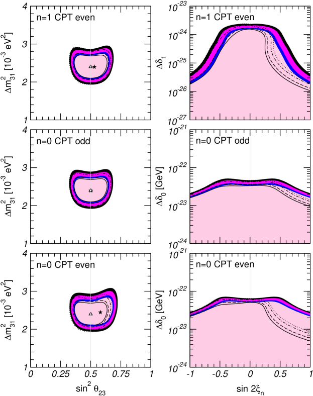
Figure 22: Allowed parameter regions for the analysis of atmospheric and LBL data in presence of $\nu_{\mu}\to\nu_{\tau}$ oscillations and different new physics effects as labeled in the figure. Each panel shows a two-dimensional projection of the allowed five-dimensional region after marginalization with respect to the three undisplayed parameters. The different contours correspond to the two-dimensional allowed regions at 90%, 95%, 99% and $3\sigma$ CL. The filled areas in the left panels show the projected two-dimensional allowed region on the oscillation parameters $\Delta m^{2}$–$\sin^{2}\theta$ plane. The best fit point is marked with a star. For the sake of comparison we also show the lines corresponding to the contours in the absence of new physics and mark with a triangle the position of the best fit point. The results are shown for the chosen relative sign $\sigma_{n}^{+}=+1$; for $\sigma_{n}^{+}=-1$ the corresponding region would be obtained by $\sin^{2}\theta\to 1-\sin^{2}\theta$. The regions on the right panels show the allowed values for the parameters characterizing the strength and mixing of the new physics. The full regions corresponds to arbitrary values of the phase $\eta_{n}$ while the lines correspond to the case $\eta_{n}\in\{0,\,\pi\}$.

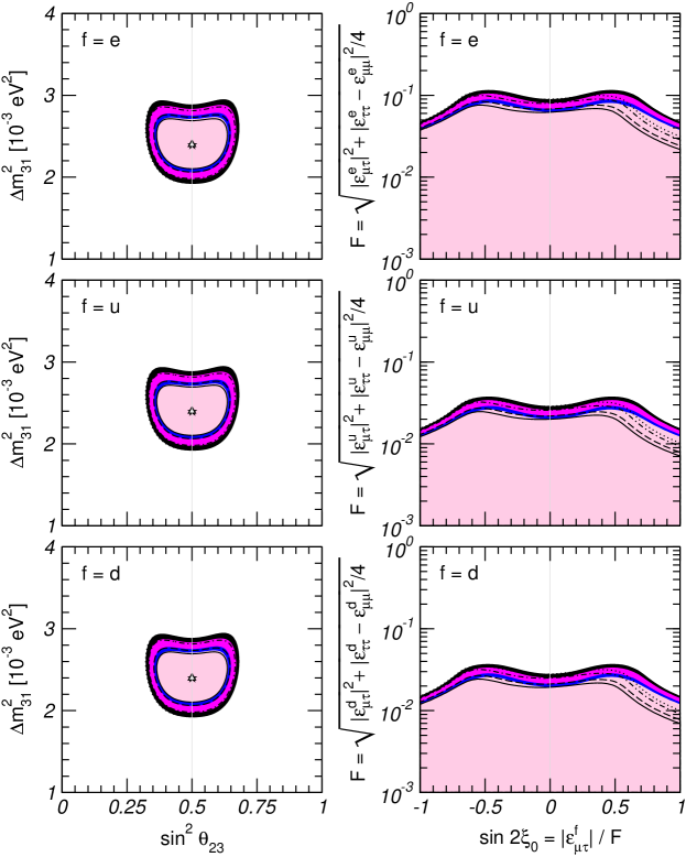
Figure 23: Same as Fig. 22 for the case of $\text{$\Delta m^{2}$-OSC}+\text{NSI}$.

From the figures we see that the best fit point is always very near the best fit point of pure $\Delta m^{2}$-OSC. In other words, the data does not show any evidence of presence of new physics even as a sub-dominant effect. Consequently the analysis allow us to derive well-defined upper bounds on the new physics parameters. The figures also illustrate that generically the bounds on $\Delta\delta_{n}$ tightens for larger values of $\xi_{n}$, being this effect stronger for effects leading to sub-dominant oscillations with stronger energy dependence. Imposing that the Hamiltonian is real does not substantially affect these conclusions.

Altogether the analysis of atmospheric and LBL neutrino data allows to impose the following at 90% ($3\sigma$) bounds on possible VLI in the $\nu_{\mu}$–$\nu_{\tau}$ sector via CPT-even effects:

$$\frac{|\Delta c|}{c}\leq 1.3\times 10^{-24}~{}(2.1\times 10^{-24})\,,$$ (167)

and on the possible VEP:

$$|\phi\,\Delta\gamma|\leq 6.3\times 10^{-25}~{}(1.0\times 10^{-24})\,.$$ (168)

$\nu_{\mu}$–$\nu_{\tau}$ the VLI via CPT-odd effects is constrained to

$$|\delta b|\leq 2.9\times 10^{-23}~{}(4.6\times 10^{-23})~{}\text{GeV}\,,$$ (169)

and non-universality of the neutrino couplings to a torsion field verify

$$|Q\,\delta k|\leq 4.7\times 10^{-23}~{}(6.6\times 10^{-23})~{}\text{GeV}.$$ (170)

For the case of non-standard neutrino interactions the corresponding 90% ($3\sigma$) bounds read:

$$(-0.058)\;{-0.038}\leq\varepsilon_{\mu\tau}^{e} \leq 0.024\;(0.043)\,, \qquad|\varepsilon_{\tau\tau}^{e}-\varepsilon_{\mu\mu}^{e}| \leq 0.11\;(0.17)\,,$$ (171)

$$(-0.019)\;{-0.012}\leq\varepsilon_{\mu\tau}^{u} \leq 0.008\;(0.014)\,, \qquad|\varepsilon_{\tau\tau}^{u}-\varepsilon_{\mu\mu}^{u}| \leq 0.036\;(0.056)\,,$$

$$(-0.019)\;{-0.012}\leq\varepsilon_{\mu\tau}^{d} \leq 0.008\;(0.014)\,, \qquad|\varepsilon_{\tau\tau}^{d}-\varepsilon_{\mu\mu}^{d}| \leq 0.035\;(0.054)$$

for real NSI, and

$$|\varepsilon_{\mu\tau}^{e}| \leq 0.038\;(0.058)\,, \qquad|\varepsilon_{\tau\tau}^{e}-\varepsilon_{\mu\mu}^{e}| \leq 0.12\;(0.19)\,,$$ (172)

$$|\varepsilon_{\mu\tau}^{u}| \leq 0.012\;(0.019)\,, \qquad|\varepsilon_{\tau\tau}^{u}-\varepsilon_{\mu\mu}^{u}| \leq 0.039\;(0.061)\,,$$

$$|\varepsilon_{\mu\tau}^{d}| \leq 0.012\;(0.019)\,, \qquad|\varepsilon_{\tau\tau}^{d}-\varepsilon_{\mu\mu}^{d}| \leq 0.038\;(0.060)$$

for the general case of complex $\varepsilon_{\mu\tau}^{f}$. Note that the different chemical composition of the Earth mantle and core have very little impact on NSI: from Fig. 23 and Eqs. (171) and (172) we see immediately that the bounds on $\varepsilon_{\alpha\beta}^{u}$ are practically identical to those on $\varepsilon_{\alpha\beta}^{d}$, and are three times stronger than those on $\varepsilon_{\alpha\beta}^{e}$. It is therefore convenient to define:

$$\varepsilon_{\alpha\beta}\equiv\sum_{f}\left<\frac{Y_{f}}{Y_{e}}\right>\varepsilon_{\alpha\beta}^{f}\approx\varepsilon_{\alpha\beta}^{e}+3\varepsilon_{\alpha\beta}^{u}+3\varepsilon_{\alpha\beta}^{d}$$ (173)

which allows to generalize the former results to the case where non-standard interactions with electrons, up-type quarks and down-type quarks are present simultaneously. By construction, the bounds and allowed regions for the effective parameters $\varepsilon_{\alpha\beta}$ coincide with those for $\varepsilon_{\alpha\beta}^{e}$ shown in Eqs. (171) and (172) and in Fig. 23.

5.3 Non-standard Neutrino Interactions in the $\nu_{e}\leftrightarrow\nu_{\tau}$ Channel

The case of non-standard neutrino interactions in the $\nu_{\mu}\leftrightarrow\nu_{\tau}$ channel considered in the previous section is only a special case of the most general scenario where all the known neutrino flavors have non-standard interactions with matter. Neglecting the solar mass splitting, $\Delta m_{21}^{2}$, and setting $\theta_{13}$ to zero, the evolution of the neutrino system is described by the Hamiltonian:

$$H_{\pm}=\frac{\Delta m^{2}_{31}}{4E}\begin{pmatrix}-1&0&0\\ 0&-\cos 2\theta_{23}&\sin 2\theta_{23}\\ 0&\hphantom{-}\sin 2\theta_{23}&\cos 2\theta_{23}\end{pmatrix}\pm\sqrt{2}G_{F}N_{e}(r)\begin{pmatrix}1+\varepsilon_{ee}^{\pm}&\varepsilon_{e\mu}^{\pm}&\varepsilon_{e\tau}^{\pm}\\ \varepsilon_{e\mu}^{\pm\star}&\varepsilon_{\mu\mu}^{\pm}&\varepsilon_{\mu\tau}^{\pm}\\ \varepsilon_{e\tau}^{\pm\star}&\varepsilon_{\mu\tau}^{\pm\star}&\varepsilon_{\tau\tau}^{\pm}\end{pmatrix}$$ (174)

Neutrino scattering tests, like those of NuTeV [189] and CHARM [190], mainly constrain the NSI couplings of the muon neutrino: $|\varepsilon_{e\mu}|\lesssim 10^{-3}$ and $|\varepsilon_{\mu\mu}|\lesssim 10^{-3}-10^{-2}$. The limits they place on $\varepsilon_{ee}$, $\varepsilon_{e\tau}$, and $\varepsilon_{\tau\tau}$ are rather loose, e.g., $|\varepsilon_{\tau\tau}^{uR}|<3$, $-0.4<\varepsilon_{ee}^{uR}<0.7$, $|\varepsilon_{\tau e}^{u}|<0.5$, $|\varepsilon_{\tau e}^{d}|<0.5$ [191].

Given the above bounds one can safely set $\varepsilon_{e\mu}$ and $\varepsilon_{\mu\mu}$ to zero in the analysis. Furthermore, motivated by the results of the previous section also $\varepsilon_{\mu\tau}$ can be neglected. In this approximation, the Hamiltonian contains five parameters: $\Delta m^{2}_{31}$ and $\theta_{23}$ and three NSI couplings $\varepsilon_{\tau\tau}$, $\varepsilon_{ee}$, and $\varepsilon_{e\tau}$ these last two giving the new three-neutrino mixing effects.

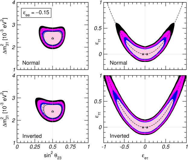
Figure 24: Same as Fig. 22 for the case of non-standard neutrino interactions in the $\nu_{e}\leftrightarrow\nu_{\tau}$ channel. Upper (lower) panels correspond to the case of normal (inverted) mass hierarchy. The black dashed lines in the right panels correspond to the parabola $(1+\varepsilon_{ee})\,\varepsilon_{\tau\tau}=|\varepsilon_{e\tau}|^{2}$ defined in Eq. (175).

As illustration of the effects due to the presence of these two new couplings we show in Fig. 24 the results of the atmospheric and LBL neutrino analysis of Ref. [192] in which for simplicity a fixed value $\varepsilon_{ee}=-0.15$ was set. The complete analysis of the full parameter space, as well as a discussion of subleading effects due to non-zero $\theta_{13}$ and $\Delta m^{2}_{21}$, can be found in [193, 194]. Comparing with Fig. 23 we see that the presence of NSI in the $\nu_{e}\leftrightarrow\nu_{\tau}$ channel allows for the relaxation of the lower bound on $\theta_{23}$, especially for the case of inverted hierarchy. On the other hand, the determination of $\Delta m^{2}_{31}$ is robust. However, the most differentiating feature is the appearance of a line in the $(\varepsilon_{e\tau},\,\varepsilon_{\tau\tau})$ plane where the effects of NSI cancel to a great extent, so that the fit is quite good even for large values of $\varepsilon_{e\tau}$ and $\varepsilon_{\tau\tau}$.

These features can be understood as follows. In the high energy limit, $E\gtrsim 10$ GeV, $\sqrt{2}G_{F}N_{e}\gg\Delta m_{31}^{2}/4E$, so for large values of the NSI parameters the matter term in the Hamiltonian (174) dominates over the vacuum term. In general, the presence of large matter effects produces deformations of the energy spectrum and therefore spoils the accurate description of the data provided by the pure vacuum solution. This is the reason why most of the points in the $(\varepsilon_{\mu\tau},\,\varepsilon_{\tau\tau})$ plane are excluded. However, along the parabola:

$$(1+\varepsilon_{ee})\,\varepsilon_{\tau\tau}=|\varepsilon_{e\tau}|^{2}\,,$$ (175)

the matter term in $H_{\pm}$ has two degenerate eigenvalues, meaning that there is a two-dimensional subspace where the NSI effects vanishes. In this subspace, neutrino oscillations exhibit the $1/E$ behavior typical of vacuum oscillations, and a good fit of the data is possible at the price of a shift in the oscillation parameters to lower values of $\theta_{23}$ and larger values of $\Delta m_{31}^{2}$. Such a shift is responsible for the extension to lower mixing angles of the allowed region in the $(\Delta m_{31}^{2},\,\theta_{23})$ plane, and introduce a tension with low-energy data (which are only marginally affected by NSI, and therefore favor the “standard” values of $\Delta m_{31}^{2}$ and $\theta_{23}$) which eventually cut the otherwise infinite parabola of degenerate solutions.

The main conclusion is that in this case it is possible to find regions of parameters in which the new physics effects cancel in the existing observables. As a consequence, while giving no positive evidence for non-standard physics the data cannot exclude large NSI. For example the $3\sigma$ bound $|\varepsilon_{\tau\tau}|<0.17$ described in the previous section can be significantly relaxed by the addition of nonzero $\varepsilon_{e\tau}$ and $\varepsilon_{ee}$, and values as large as $\varepsilon_{\tau\tau}\sim 1$ are allowed.

5.4 Damping Effects in $\nu_{\mu}\rightarrow\nu_{\tau}$ Oscillations: Decay and Decoherence

We describe in this section the phenomenology of atmospheric neutrino flavor mixing in the presence of new physics effects which, unlike those described in Sec. 5.1, lead to a decrease with time of the oscillation amplitude. In particular we will concentrate on the possibility of neutrino decay and of non-standard physics leading to quantum decoherence.

For the sake of concreteness, when discussing neutrino decay, we will focus on scenarios in which only the heaviest neutrino ($\nu_{3}$ by convention) decays and its decay is invisible so that the decay products are either outside of the $\nu_{\mu}$ $\nu_{\tau}$ neutrino ensemble or their are so degraded in energy that they do not contribute to the observed event rates and they are fast enough to have interesting effects in atmospheric neutrino phenomenology

Fast invisible neutrino decay for $\nu_{3}$ to $\nu_{i}$ Majorana neutrinos can be induced by the effective interaction:

$$\mathcal{L}_{I}=g_{i3}\,\bar{\nu}_{iL}^{c}\,\nu_{3L}\ ,J+\text{h.c.}\,,$$ (176)

where $J$ is the Majoron field [195, 196, 197, 198, 199, 200], which has to be dominantly singlet with only a small triplet admixture, in order to satisfy the constraints from the invisible decay width of $Z$ [201].

A decay model for Dirac neutrinos can also be constructed via the coupling between the right–handed $SU(2)$–singlet states given by [202]

$$\mathcal{L}_{I}=g_{i3}\,\bar{\nu}_{iR}^{c}\,\nu_{3R}\,\chi+\text{h.c.}\,,$$ (177)

where $\chi$ is a complex scalar field with lepton number $-2$, $I_{W}=0$, and hypercharge zero and which should be light compared to the neutrino masses.

With the interaction of Eq. (177) or Eq. (176), the rest-frame lifetime of $\nu_{3}$ is given by

$$\tau_{3}=\frac{16\pi}{g_{i3}^{2}}\frac{m_{3}^{3}}{\Delta m^{2}_{3i}(m_{3}+m_{i})^{2}}\,,$$ (178)

Furthermore it can be shown that the mass difference between the decaying neutrino and the daughter one has to verify that

$$\Delta m^{2}_{3j}>0.73~{}\text{eV}^{2}\,,$$ (179)

to satisfy constraints from $K\to\mu+\text{neutrals}$ decay [174].

With these assumptions neutrino decay can be accounted for in the evolution equation by introducing an imaginary part in the Hamiltonian which is proportional to the decay width:

$$i\,\frac{d\vec{\nu}}{dx}=U\left[\frac{\Delta m_{31}^{2}}{4E}\begin{pmatrix}-1&0\\ \hphantom{-}0&~{}1\end{pmatrix}-i\frac{m_{3}}{2\,\tau_{3}\,E}\begin{pmatrix}0&0\\ 0&1\end{pmatrix}\right]U^{\dagger}\,\vec{\nu}\,,$$ (180)

where $\tau_{3}$ is the $\nu_{3}$ lifetime.

Solving Eq. (180) one gets the survival probability of $\nu_{\mu}$ as given by:

$$P(\nu_{\mu}\to\nu_{\mu})=\cos^{4}\theta_{23}+\sin^{4}\theta_{23}e^{-\frac{m_{3}\,L}{\tau_{3}\,E}}\\ +2\sin^{2}\theta_{23}\cos^{2}\theta_{23}e^{-\frac{m_{3}\,L}{2\tau_{3}\,E}}\cos\left(\frac{\Delta m_{31}^{2}L}{2E}\right)\,.$$ (181)

As mentioned above, Eq. (181) can describe for example the decay $\nu_{3}\rightarrow\bar{\nu}_{1,2}+J(\chi)$. In this case the mass difference between the decaying state and the daughter state is the same as in Eq. (181). Therefore the constraint Eq. (179) implies that the oscillating term in Eq. (181) averages to zero and $P(\nu_{\mu}\to\nu_{\mu})$ simplifies to

$$P(\nu_{\mu}\to\nu_{\mu})=\cos^{4}\theta_{23}+\sin^{4}\theta_{23}e^{-\frac{m_{3}\,L}{\tau_{3}\,E}}.$$ (182)

This decay scenario was proposed in Ref. [174] where it was found that it could describe the $L/E_{\nu}$ dependence and the asymmetry of the contained events in Super-Kamiokande if $\sin^{2}\theta_{23}\sim 0.87$ and $m_{3}/\tau_{3}\sim 1~{}\text{GeV}/D_{E}$ (where $D_{E}$ is the diameter of the Earth).

However, when studied in detail, it was shown that the description of the global contained event sample in this scenario is worse than in the case of oscillations. This arises from the strong energy dependence of the survival probability while the contained data both in the sub-GeV and multi-GeV samples present a similar deficit. As a consequence the allowed decay lifetimes which give a good description to the sub-GeV and multi-GeV data are not the same and the decay hypothesis cannot produce enough up-down asymmetry for the multi-GeV sample without conflicting with the sub-GeV data.

This behavior becomes particularly lethal when trying to describe the upward going muon data since for lifetimes favored by the contained event data very little muon conversion is expected already for stopping muons in contradiction with observation. Based on this fact this mechanism was ruled out in its simpler form in Refs. [182, 184].

Another possibility, mentioned in Ref. [174] and developed in Ref. [175] was the decay of $\nu_{3}$ is into a state $\nu_{j}$ with which it does not mix. In this case, the $\Delta m_{31}^{2}$ in Eq. (181) is not directly related to the mass difference between the decaying state and the daughter neutrino. Consequently $\Delta m_{31}^{2}$ can be taken to be very small for all energy ranges relevant for atmospheric neutrinos ($\Delta m^{2}_{31}<10^{-4}~{}\text{eV}^{2}$) so that the the oscillating term in Eq. (181) is one and $P(\nu_{\mu}\to\nu_{\mu})$ becomes

$$P(\nu_{\mu}\to\nu_{\mu})=\left(\cos^{2}\theta_{23}+\sin^{2}\theta_{23}e^{-\frac{m_{3}\,L}{2\tau_{3}\,E}}\right)^{2}\,.$$ (183)

This scenario was explored in detail in Ref. [175] where it was found that a good fit to the contained and upgoing muon atmospheric data at that time could be obtained for the choice of parameters

$$\tau_{3}/m_{3}=63~{}\text{km/GeV},\qquad\sin^{2}\theta_{23}=0.30\,.$$ (184)

In Ref. [203] Super-Kamiokande collaboration presented the study of the muon neutrino disappearance probability as a function of neutrino flight length L over neutrino energy E. They found a dip in the L/E distribution, as predicted from the sinusoidal flavor transition probability of neutrino oscillation. This analysis found that the decay probability in Eq. (183) provided a worse fit (by about $3.4\sigma$) than the pure oscillation hypothesis to the observed distribution.

Another mechanism that was proposed as a modification to the oscillation pattern was the possibility of new sources of quantum decoherence. Quantum gravity, as suggested by Hawking in the context of black-hole thermodynamics [204] could provide a source for this effect. In this approach any physical system is inherently “open”, due to its unavoidable, decohering interactions with a pervasive “environment” (the spacetime and its Planck-scale dynamics [205, 206]). In Ref. [176] this mechanism was studied as an alternative interpretation of the atmospheric neutrino data as we briefly summarize here.

In order to include decoherence effects in the neutrino flavor oscillation equations it is convenient to use the density matrix formalism. In this formalism the evolution of the neutrino ensemble is determined by the Liouville equation for the density matrix $\rho(t)=\nu(t)\otimes\nu(t)^{\dagger}$

$$\frac{d\rho}{dx}=-i[H,\,\rho]\,,$$ (185)

where $H$ is given by Eq. (149). The survival probability in Eq. (156) is given by $P_{\mu\mu}(t)=\mathop{\mathrm{Tr}}[\Pi_{\nu_{\mu}}\,\rho(t)]$, where $\Pi_{\nu_{\mu}}=\nu_{\mu}\otimes\nu_{\mu}$ is the $\nu_{\mu}$ state projector, and with initial condition $\rho(0)=\Pi_{\nu_{\mu}}$. An equivalent equation can be written for the antineutrino density matrix.

For the case of oscillations between two neutrino states the hermitian operators $\rho$, $H$ and the flavor projectors $\Pi_{\nu_{\mu}}$ and $\Pi_{\nu_{\tau}}$ can be expanded in the basis formed by the unit matrix and the three Pauli matrices $\sigma_{i}$. In particular we can write

$$\rho(x)=\frac{1}{2}\big{[}I+\vec{p}(x)\cdot\vec{\sigma}\big{]}\,,\qquad H=\frac{1}{2}\vec{h}\cdot\vec{\sigma}\,,$$ (186)

and the evolution of the neutrino ensemble is determined by a precession-like equation of the three-vector $\vec{p}(t)$

$$\frac{d\vec{p}}{dx}=\vec{p}(x)\times\vec{h}\,.$$ (187)

In this language modifications of Eq. (185) which emerge from dissipative interactions with an environment can be parametrized by introducing an extra term $\mathcal{D}[\rho]$,

$$\frac{d\rho}{dx}=-i[H,\,\rho]-\mathcal{D}[\rho]\,,$$ (188)

which violates the conservation of $\mathop{\mathrm{Tr}}(\rho^{2})$ and allows transitions from pure to mixed states. The operator $\mathcal{D}$ has the dimension of an energy, and its inverse defines the typical (coherence) length after which the system gets mixed.

In Ref. [176] it was assumed that the decoherence term took the Lindblad form [207]

$$\mathcal{D}[\rho]=\sum_{n}\{\rho,\,D_{n}\,D_{n}^{\dagger}\}-2D_{n}\,\rho\,D^{\dagger}_{n}\,,$$ (189)

which arises from the requirement of complete positivity [208] as implied by a a linear, Markovian, and trace-preserving map $\rho(0)\to\rho(t)$.

In Eq. (189) the operators $D_{n}$ arise from tracing away the environment dynamics and here they parametrize the new physics effects. for which there are no first-principle calculations. Consequently, in Ref. [176] a phenomenological approach was taken in which it was simply required that the $\nu$ system obeys the laws of thermodynamics: the increase of the entropy and the conservation of the average energy. These two requirements imply that:

$$D_{n}=D^{\dagger}_{n}\qquad\text{and}\qquad[H,\,D_{n}]=0\,,$$ (190)

so that Eq. (189) becomes

$$\mathcal{D}[\rho]=\sum_{n}\,[D_{n},\,[D_{n},\,\rho]]\,.$$ (191)

As it was discussed above for the case of oscillations, the hermitian operators $\rho$, $\Pi_{\nu_{\mu}}$, $H$, and $D_{n}$, can be expanded onto the basis formed by the unit matrix and the three Pauli matrices so that in addition to Eq. (186) we can write

$$D_{n}=\frac{1}{2}\vec{d}_{n}\cdot\vec{\sigma}\,,$$ (192)

with this Eq. (188) can be then written as a Bloch equation,

$$\frac{d\vec{p}}{dx}=\vec{p}(x)\times\vec{h}-G\cdot\vec{p}\,,$$ (193)

where the tensor ${G}=\sum_{n}|\vec{d}_{n}|^{2}\,I-\vec{d}_{n}\otimes\vec{d}_{n}^{T}$. This equation has a simple physical interpretation: the first term induces flavor oscillations, as discussed above, while the decoherence term ${G}\cdot\vec{p}$ is responsible for their damping.

The requirement of conservation of the average energy, $[H,\,D_{n}]=0$, implies that each vector $\vec{d}_{n}$ is parallel to $\vec{h}$. Therefore, the tensor ${G}$ takes the form

$$G=\mathop{\mathrm{diag}}(\gamma,\,\gamma,\,0)\qquad\text{with}\qquad\gamma=\sum_{n}|\vec{d}_{n}|^{2}\,.$$ (194)

With this the $\nu_{\mu}$ survival probability takes the form

$$P_{\mu\mu}=1-\frac{1}{2}\sin^{2}2\theta_{23}\left[1-e^{-\gamma L}\cos\left(\frac{\Delta m^{2}_{31}L}{2E}\right)\right]\,.$$ (195)

The L/E analysis of SK [203] disfavored the pure decoherence scenario (corresponding to the limit $\Delta m^{2}_{31}=0$ in Eq. (195)) by about $3.8\sigma$ when compared to the pure oscillation case. In Ref. [185] a global analysis to the Super-Kamiokande and first K2K data was performed allowing for simultaneous oscillations and decoherence effects as described by Eq. (195). They found that the best fit was obtained by the pure oscillation scenario so that no evidence for decoherence effects was present in the data. Conversely the analysis allowed to set an upper bound on the decoherence parameter

$$\gamma^{2}\lesssim 3\times 10^{-3}~{}\text{eV}^{2}\,,$$ (196)

at $3\sigma$.

It is interesting to notice that both neutrino decay and decoherence lead to an exponentially decreasing $P_{\mu\mu}$ which is qualitatively similar as can be seen by comparing Eq. (181) and Eq. (195). Consequently the decay and decoherence scenarios cannot be easily distinguished in $\nu_{\mu}$ disappearance. However, they can be distinguished through the appearance modes, i.e., through neutral current (NC) events and $\tau$ appearance events in SK. This is so because in the in the decoherence case the total number of active neutrinos is conserved while in the decay scenario it decreases with L/E.

5.5 Effects at Neutrino Telescopes: Propagation in Matter of High Energy Oscillating Neutrinos

In contrast to the $E$ energy dependence of the conventional oscillation length, the new physics scenarios that we discussed in Sec. 5.1 predict neutrino oscillations with wavelengths that are constant or decrease with energy. Therefore the effects are more visible at higher energies.

Neutrino telescopes [209] are underwater or under-ice devices aimed at detecting high energy neutrinos from distant sources. In neutrino telescopes, neutrinos are detected through the observation of Cherenkov light emitted by charged particles produced in neutrino interactions. The neutrino induced events can be categorized as either muon tracks or showers. Cosmic ray muons and muons from CC $\nu_{\mu}$ interactions are the origin of tracks. Showers results from neutrino interactions –  $\nu_{e}$ or $\nu_{\tau}$ CC interactions, and NC interactions initiated by all three flavors – inside or near the detector. Because of the large range of muons, kilometers to tens of kilometers for the energies considered, the effective volume of the detector for muon neutrinos is significantly larger than the instrumented volume. Furthermore, the angular resolution for muon tracks is superior to that for showers.

Despite their main goal is the observation of neutrinos of extraterrestrial origin, a neutrino telescope can also detect atmospheric neutrinos which, as a matter of fact, constitute the main background in their searches for astrophysical sources. However, as it is many times the case in particle physics experiments, the study of the background can still leave an important room for discovery. Indeed neutrino telescopes, with an energy reach in the $0.1\sim 10^{4}$ TeV range for atmospheric neutrinos, are also ideal instruments to search for the new physics effects discussed above. For most of this energy interval standard $\Delta m^{2}$ oscillations are suppressed and therefore the observation of an angular distortion of the atmospheric neutrino flux or its energy dependence provide a clear signature for the presence of new physics mixing neutrino flavors.

The Hamiltonian of Eq. (149) describes the coherent evolution of the $\nu_{\mu}$–$\nu_{\tau}$ ensemble for any neutrino energy. But high-energy neutrinos propagating in the Earth can also interact inelastically with the Earth matter either by CC and NC and as a consequence the neutrino flux is attenuated. This attenuation is qualitatively and quantitatively different for $\nu_{\tau}$’s and $\nu_{\mu}$’s. Muon neutrinos are absorbed by CC interactions while tau neutrinos are regenerated because they produce a $\tau$ that decays into another tau neutrino before losing energy [210]. As a consequence, for each $\nu_{\tau}$ lost in CC interactions, another $\nu_{\tau}$ appears (degraded in energy) from the $\tau$ decay and the Earth never becomes opaque to $\nu_{\tau}^{\prime}s$. Furthermore, as pointed out in Ref. [211], a new secondary flux of $\bar{\nu}_{\mu}$’s is also generated in the leptonic decay $\tau\rightarrow\mu\bar{\nu}_{\mu}\nu_{\tau}$.

Attenuation and regeneration effects of incoherent neutrino fluxes can be consistently described by a set of coupled partial integro-differential cascade equations (see for example [212, 213, 214, 215] and references therein). In this way, for example, the observed $\nu_{\mu}$ and oscillation-induced $\nu_{\tau}$ fluxes (and the associated event rates in a high energy neutrino telescope) from astrophysical sources has been evaluated. Alternatively, these effects can be accounted for in a Monte Carlo simulation of the neutrino propagation in matter [210, 211, 216]. Whatever the technique used, because of the long distance traveled by the neutrinos from the source, the oscillations average out and the neutrinos arriving at the Earth can be treated as an incoherent superposition of mass eigenstates.

For atmospheric neutrinos this is not the case because oscillation, attenuation, and regeneration effects occur simultaneously when the neutrino beam travels across the Earth’s matter. For the phenomenological analysis of conventional neutrino oscillations this fact can be ignored because the neutrino energies covered by current experiments are low enough for attenuation and regeneration effects to be negligible. Especially for non-standard scenario oscillations, future experiments probe high-energy neutrinos for which the attenuation and regeneration effects have to be accounted for simultaneously.

In order to include all these effects in the neutrino flavor oscillation equations it is convenient to use the density matrix formalism as introduced in the previous section. In this formalism attenuation effects due to CC and NC interactions can be introduced by relaxing the condition $\mathop{\mathrm{Tr}}(\rho)=1$. In this case

$$\rho(x)=\frac{1}{2}\big{[}p_{0}(x)+\vec{p}(x)\cdot\vec{\sigma}\big{]}\,,$$ (197)

and

$$\frac{d\rho(E,x)}{dx}=-i\big{[}H(E),\;\rho(E,x)\big{]}-\sum_{\alpha}\frac{1}{2\lambda^{\alpha}_{\text{int}}(E,x)}\big{\{}\Pi_{\alpha},\,\rho(E,x)\big{\}}\,,$$ (198)

where we have explicitly exhibited the energy dependence and

$$[\lambda^{\alpha}_{\text{int}}(E,x)]^{-1} \equiv[\lambda^{\alpha}_{\text{CC}}(E,x)]^{-1}+[\lambda_{\text{NC}}(E,x)]^{-1}\,,$$ (199)

$$[\lambda^{\alpha}_{\text{CC}}(E,x)]^{-1} =n_{T}(x)\,\sigma^{\alpha}_{\text{CC}}(E)\,,$$

$$[\lambda_{\text{NC}}(E,x)]^{-1} =n_{T}(x)\,\sigma_{\text{NC}}(E)\,.$$

$n_{T}(x)$ is the number density of nucleons at the point $x=ct$. $\sigma^{\alpha}_{\text{CC}}(E)$ is the cross section for CC interaction, $\nu_{\alpha}+N\rightarrow l_{\alpha}+X$, and $\sigma_{\text{NC}}(E)$ is the cross section for $\nu_{\alpha}+N\rightarrow\nu_{\alpha}+X$ which is flavor independent. Thus we obtain four equations that describe the evolution of the neutrino system because one has to take into account both the flavor precession of the vector $\vec{p}(E,t)$ as well as the neutrino intensity attenuation encrypted in the evolution of $p_{0}(E,t)$.

$\nu_{\tau}$ regeneration and neutrino energy degradation can be accounted for by coupling these equations to the shower equations for the $\tau$ flux, $F_{\tau}(E_{\tau},t)$ (we denote by $F$ the differential fluxes $d\phi/(dE\,d\cos\theta)$). Muons decouple from the evolution equations because they range out electromagnetically in the Earth matter before they can produce a $\nu_{\mu}$ by decay or CC interaction. It is convenient to define the neutrino flux density matrix $F_{\nu}(E,x)=F_{\nu_{\mu}}(E,x_{0})\,\rho(E,x)$ where $F_{\nu_{\mu}}(E,x_{0})$ is the initial neutrino flux. The equations can be written as:

$$\begin{split}\frac{dF_{\nu}(E_{\nu},x)}{dx}&=-i\big{[}H,\,F_{\nu}(E_{\nu},x)\big{]}-\sum_{\alpha}\frac{1}{2\lambda^{\alpha}_{\text{int}}(E_{\nu},x)}\big{\{}\Pi_{\alpha},\,F_{\nu}(E_{\nu},x)\big{\}}\\ &\hskip 14.22636pt+\int_{E_{\nu}}^{\infty}\frac{1}{\lambda_{\text{NC}}(E^{\prime}_{\nu},x)}F_{\nu}(E^{\prime}_{\nu},x)\frac{dN_{\text{NC}}(E^{\prime}_{\nu},E_{\nu})}{dE_{\nu}}dE^{\prime}_{\nu}\\ &\hskip 14.22636pt+\int_{E_{\nu}}^{\infty}\frac{1}{\lambda^{\tau}_{\text{dec}}(E_{\tau},x)}F_{\tau}(E_{\tau},x)\frac{dN_{\text{dec}}(E_{\tau},E_{\nu})}{dE_{\nu}}dE_{\tau}\,\Pi_{\tau}\\ &\hskip 14.22636pt+\text{Br}_{\mu}\,\int_{E_{\nu}}^{\infty}\frac{1}{\lambda^{\tau}_{\text{dec}}(E_{\tau},x)}\,\bar{F}_{\tau}(\bar{E}_{\tau},x)\frac{d\bar{N}_{\text{dec}}(\bar{E}_{\tau},E_{\nu})}{dE_{\nu}}d\bar{E}_{\tau}\,\Pi_{\tau}\,,\end{split}$$ (200)

$$\begin{split}\frac{dF_{\tau}(E_{\tau},t)}{d\,x}&=-\frac{1}{\lambda^{\tau}_{\text{dec}}(E_{\tau},x)}F_{\tau}(E_{\tau},x)\\ &\hskip 14.22636pt+\int_{E_{\tau}}^{\infty}\frac{1}{\lambda^{\tau}_{\text{CC}}(E_{\nu},t)}\mathop{\mathrm{Tr}}\big{[}\Pi_{\tau}\,{F_{\nu}}(E_{\nu},t)\big{]}\frac{dN_{\text{CC}}(E_{\nu},E_{\tau})}{dE_{\tau}}dE_{\nu}\,.\end{split}$$ (201)

$\lambda^{\tau}_{\text{dec}}(E_{\tau},x)=\gamma_{\tau}\,c\,\tau_{\tau}$. $\tau_{\tau}$ is the $\tau$ lifetime and $\gamma_{\tau}=E_{\tau}/m_{\tau}$ is its gamma factor.

The CC and NC distributions are defined as:

$$\frac{dN_{\text{NC}}(E^{\prime}_{\nu},E_{\nu})}{dE_{\nu}} \equiv\frac{1}{\sigma_{\text{NC}}(E^{\prime}_{\nu})}\frac{d\sigma_{\text{NC}}(E^{\prime}_{\nu},E_{\nu})}{dE_{\nu}}\,,$$ (202)

$$\frac{dN_{\text{CC}}(E_{\nu},E_{\tau})}{dE_{\tau}} \equiv\frac{1}{\sigma^{\tau}_{\text{CC}}(E_{\nu})}\frac{d\sigma^{\tau}_{\text{CC}}(E_{\nu},E_{\tau})}{dE_{\tau}}\,,$$

The $\tau$ decay distribution $\frac{dN_{\text{dec}}(E_{\tau},E_{\nu})}{dE_{\nu}}$ can be found, for example, in Ref. [212] and $\frac{d\bar{N}_{\text{dec}}(\bar{E}_{\tau},E_{\nu})}{dE_{\nu}}$ in Ref. [19].

The third term in Eq. (200) represents the neutrino regeneration by NC interactions and the fourth term represents the contribution from $\nu_{\tau}$ regeneration, $\nu_{\tau}\rightarrow\tau^{-}\rightarrow\nu_{\tau}$, describing the energy degradation in the process. The secondary $\nu_{\mu}$ flux from $\bar{\nu}_{\tau}$ regeneration, $\bar{\nu}_{\tau}\rightarrow\tau^{+}\rightarrow\bar{\nu}_{\tau}+\mu^{+}+\nu_{\mu}$, is described by the last term where we denote by over-bar the energies and fluxes of the $\tau^{+}$. $\text{Br}_{\mu}=0.18$ is the branching ratio for this decay. In Eq. (201) the first term gives the loss of taus due to decay and the last term gives the $\tau$ generation due to CC $\nu_{\tau}$ interactions. In writing these equations the tau energy loss has been neglected because it is only relevant at much higher energies.

An equivalent set of equations can be written for the antineutrino flux density matrix and the for the $\tau^{+}$ flux. Both sets of equations are coupled due to the secondary neutrino flux term.

Figure 25: Vertically upgoing neutrinos after traveling the full length of the Earth taking into account the effects due to VLI oscillations, attenuation in the Earth, $\nu_{\tau}$ regeneration and secondary $\bar{\nu}_{\tau}$ regeneration (see text for details).

After solving this set of ten coupled evolution equations that describe propagation through the Earth one obtains the neutrino fluxes in the vicinity of the detector from

$$\frac{d\phi_{\nu_{\alpha}}(E,\theta)}{dE\,d\cos\theta}=\mathop{\mathrm{Tr}}\big{[}F_{\nu}(E,L=2R\cos\theta)\,\Pi_{\alpha}\big{]}\,.$$ (203)

Figure. 25 illustrates the interplay between the different terms in Eqs. (200) and (201). The figure covers the example of VLI-induced oscillations with $\delta c/c=10^{-27}$ and maximal $\xi_{vli}$ mixing. The upper panels show the final $\nu_{\mu}$ and $\nu_{\tau}$ fluxes for vertically upgoing neutrinos after traveling the full length of the Earth for the initial conditions $d\Phi(\nu_{\mu})_{0}/dE_{\nu}=d\Phi(\bar{\nu}_{\mu})_{0}/dE_{\nu}\propto E^{-1}$ and $d\Phi(\nu_{\tau})_{0}/dE_{\nu}=d\Phi(\bar{\nu}_{\tau})_{0}/dE_{\nu}=0$.

The figure illustrates that the attenuation in the Earth suppresses the neutrino fluxes at higher energies. The effect of the attenuation in the absence of oscillations is given by the dotted thin line in the left panel. Even in the presence of oscillations this effect can be well described by an overall exponential suppression [19, 217] both for $\nu_{\mu}$’s and the oscillated $\nu_{\tau}$’s. In other words, the curve for “oscillation + attenuation” can be reproduced simply by multiplying the initial flux by the oscillation probability and an exponential damping factor:

$$\frac{d\phi_{\nu_{\alpha}}(E,\theta,L=2R\cos\theta)}{dEd\cos\theta}=\frac{d\phi_{\nu_{\mu},0}(E,\theta)}{dEd\cos\theta}\,P_{\mu\alpha}(E,L=2R\cos\theta)\\ \times\exp\big{\{}-X(\theta)[\sigma_{\text{NC}}(E)+\sigma_{\text{CC}}^{\alpha}(E)]\big{\}}\,,$$ (204)

where $X(\theta)$ is the column density of the Earth.

The main effect of energy degradation by NC interactions (the third term in Eq. (200)) that is not accounted for in the approximation of Eq. (204) is the increase of the flux in the oscillation minima (the flux does not vanish in the minimum) because higher energy neutrinos end up with lower energy as a consequence of the NC interactions. The difference between the dash-dotted line and the dashed line is due to the interplay between the $\nu_{\tau}$ regeneration effect (fourth term in Eq. (200)) and the flavor oscillations. As a consequence of the first effect, we see in the right upper panel that the $\nu_{\tau}$ flux is enhanced because of the regeneration of higher energy $\nu_{\tau}$’s, $\nu_{\tau}(E)\rightarrow\tau^{-}\rightarrow\nu_{\tau}(E^{\prime}<E)$, that originated from the oscillation of higher energies $\nu_{\mu}$’s. In turn this excess of $\nu_{\tau}$’s produces an excess of $\nu_{\mu}$’s after oscillation which is seen as the difference between the dashed curve and the dash-dotted curve in the left upper panel. Finally the secondary effect of $\bar{\nu}_{\tau}$ regeneration (last term in Eq. (200)), $\bar{\nu}_{\tau}(E)\rightarrow\tau^{+}\rightarrow\mu^{+}\,\bar{\nu}_{\tau}\,\nu_{\mu}(E^{\prime}<E)$, results into the larger $\nu_{\mu}$ flux (seen in the left upper panel as the difference between the dashed and the thick full lines). This, in turn, gives an enhancement in the $\nu_{\tau}$ flux after oscillations as seen in the right upper panel.

The lower panels show the final $\nu_{\mu}$ and $\nu_{\tau}$ fluxes for an atmospheric-like energy spectrum $d{\Phi(\nu_{\mu})_{0}}/dE_{\nu}=d\Phi(\bar{\nu}_{\mu})_{0}/dE_{\nu}\propto E^{-3}$ and $d\Phi(\nu_{\tau})_{0}/dE_{\nu}=d{\Phi(\bar{\nu}_{\tau})_{0}}/dE_{\nu}=0$. In this case all regeneration effects are suppressed. Regeneration effects result in the degradation of the neutrino energy and the more steeply falling the neutrino energy spectrum, the smaller the contribution to the total flux. Therefore, in this case, the final fluxes can be relatively well described by the approximation in Eq. (204).

5.5.1 Example: VLI-induced Oscillations at ICECUBE

Figure 26: Zenith angle distributions for muon induced events for different values of the VLI parameter $\Delta c/c$ and maximal mixing $\xi_{vli}=\pi/4$ for different threshold energy $E_{\mu}^{fin}>E_{\text{threshold}}$ normalized to the expectations for pure $\Delta m^{2}$ oscillations. The dashed line includes only the $\nu_{\mu}$-induced muon events and the full line includes both the $\nu_{\mu}$-induced and $\nu_{\tau}$-induced muon events.

Figure 27: Sensitivity limits in the $\Delta c/c,\,\xi_{\text{vli}}$ at 90%, 95%, 99% and $3\sigma$ CL. The hatched area in the upper right corner is the present $3\sigma$ bound from the analysis of SK+K2K+Minos data in Sec. 5.2. In order to estimate the uncertainty associated with the poorly known charm meson production cross sections at the relevant energies, the results are presented for two different models of charm production: the recombination quark parton model (RQPM) developed by Bugaev et al. [218] (filled regions) and the model of Thunman et al. (TIG) [219] (full lines) that predicts a smaller rate.

For illustration we present here the results of Ref. [220] on the physics potential of ICECUBE [221], now under construction to unravel these new physics effects. ICECUBE will consist of 80 kilometer-length strings, each instrumented with 60 10-inch photomultipliers spaced by 17 m. The deepest module is 2.4 km below the surface. The strings are arranged at the apexes of equilateral triangles 125 m on a side. The instrumented detector volume is a cubic kilometer.

The most obvious effect of neutrino oscillations induced by the new physics at ICECUBE will be an energy dependent distortion of the zenith angle distribution of atmospheric muon neutrino events. Also one has to take into account that together with $\nu_{\mu}$-induced muon events, oscillations also generate $\mu$ events from the CC interactions of the $\nu_{\tau}$ flux which reaches the detector producing a $\tau$ that subsequently decays as $\tau\rightarrow\mu\,\bar{\nu}_{\mu}\,\nu_{\tau}$ and produces a $\mu$ in the detector.

We show in Fig. 26 the zenith angle distributions for muon induced events for different values of the VLI parameter $\Delta c/c$ and maximal mixing $\xi_{vli}=\pi/4$ for different threshold energy $E_{\mu}^{fin}>E_{\text{threshold}}$ normalized to the expectations for pure $\Delta m^{2}$ oscillations. The full lines include both the $\nu_{\mu}$-induced events and $\nu_{\tau}$-induced events while the last ones are not included in the dashed curves. As seen in the figure, for a given value of $\Delta c/c$ there is a range of energy for which the angular distortion is maximal. Above that energy, the oscillations average out and result in a constant suppression of the number of events. Inclusion of the $\nu_{\tau}$-induced events events leads to an overall increase of the event rate but slightly reduces the angular distortion as a consequence of the “anti-oscillations” of the $\nu_{\tau}$’s as compared to the $\nu_{\mu}$’s. The expected sensitivity bounds which were be obtained in Ref. [220] from the statistical analysis of this distortion are shown in Fig. 27.

The figure illustrates the physics potential for discovery beyond the present bounds by more than two orders of magnitude even within the context of this very conservative analysis.

6 Non Standard Medium Effects in Solar and Reactor Neutrinos

As discussed in Sec. 5 oscillations are not the only possible mechanism for flavor transitions. They can also be generated by a variety of forms of nonstandard neutrino interactions or properties. In this section we describe some phenomenology associated with models which affect $\nu_{e}$ oscillations and which can be observed or constrained by the combined analysis of solar and KamLAND experiments.

At present solar neutrino data is the most sensitive probe that we have on flavor effects in neutrino propagation in a dense medium. On the other hand, because of the smaller density of the Earth background, such “environmental” effects are expected to be much less relevant in the oscillation of reactor $\bar{\nu}_{e}$’s observed in KamLAND. Consequently the requirement of simultaneously describing solar and KamLAND data is an important test on new physics scenarios which induce non-universal effective couplings of $\nu_{e}^{\prime}s$ to the particles in the background.

Generically in most neutrino mass models, new sources of environmental dependence (ED) of the effective neutrino mass arise as a natural feature due to the presence of non-standard neutrino interactions. The form in which the presence of the non-standard interactions affect the neutrino propagation depends on the tensor structure of the new force. If the new interaction can be cast as a neutral or charged vector current, it will contribute as an energy independent potential to the neutrino evolution equation in addition to the MSW potential of the Standard Model. On the other hand tensor neutral forces lead to an energy decreasing potential while new physics in the form of Yukawa interactions of neutrinos and matter with a neutral scalar particle modify the kinetic part of the neutrino evolution equation.

Assuming that the oscillation of solar and KamLAND antineutrinos are still dominated by a single mass scale even in the presence of these effects one can write their evolution equation as:

$$i\frac{d}{dx}\begin{pmatrix}\nu_{e}\\ \nu_{a}\end{pmatrix}=\left[\frac{1}{2E_{\nu}}U_{12}\,M^{2}(x)\,U_{12}^{\dagger}+V(x)\right]\begin{pmatrix}\nu_{e}\\ \nu_{a}\end{pmatrix}\,,$$ (205)

where we have defined $M(x)$ as the modified neutrino mass matrix which will not be diagonal and will vary along the neutrino trajectory but that is energy independent and have the same sign for neutrinos and antineutrinos. V(x) contains the standard MSW potential as well as all other effects which are not included in $M(x)$. We label $\nu_{a}=\cos\theta_{23}\nu_{\mu}+\sin\theta_{23}\nu_{\tau}$.

In what follows we illustrate the possible phenomenological consequences of the presence of new interactions in the solar neutrino oscillations in two different scenarios: mass varying neutrinos (MaVaNs) models associated to the origin of the cosmic acceleration [222, 223, 224] and the possibility of long range leptonic forces [225].

6.1 Mass Varying Neutrinos in the Sun: $\nu$ Density Effects

One of the truly challenging and open questions in both cosmology and particle physics is the nature of the dark energy in the Universe. In parallel, one would like to explain also why, in the present epoch, the energy density associated with dark energy and that of matter happen to be approximately the same if these densities have different temperature dependence. This coincidence is resolved dynamically if the dark energy density tracks (some component) of the matter density [226, 227, 228].

In Refs. [222, 223] it was proposed that the dark energy density tracks the energy density in neutrinos. This implies that the energy density associated with dark energy depends on the neutrino masses and in turn, neutrino masses are not fixed but variable with their magnitude being a function of the neutrino density.

Besides the possible interesting cosmological effects [222, 223, 229, 230, 231, 232], from the point of view of neutrino oscillation phenomenology the unavoidable consequence of these scenarios is that the neutrino mass depends on the local neutrino density and therefore can be different in media with high neutrino densities such as the Sun [233].

In the simplest realization of this scenario neutrino mass arises from the interaction with a scalar field, the acceleron, whose effective potential changes as a function of the neutrino density. For most purposes, the derivation of the effective neutrino mass in the presence of the neutrino background can be made in a model independent way using the neutrino mass $m_{\nu}$ as the dynamical field (without making explicit use of the dependence of $m_{\nu}$ on the acceleron field). In this approach at low energies the effective Lagrangian for $m_{\nu}$ is

$$\mathcal{L}=m_{\nu}\bar{\nu}^{c}\nu+V_{tot}(m_{\nu})\,,$$ (206)

where $V_{tot}(m_{\nu})=V_{\nu}(m_{\nu})+V_{0}(m_{\nu})$ contains the contribution to the energy density both from the neutrinos as well as from the scalar potential. The condition of minimization of $V_{tot}$ determines the physical neutrino mass.

The contribution of a neutrino background to the energy density is given by

$$V_{\nu}=\int\frac{d^{3}k}{(2\pi)^{3}}\,{\sqrt{k^{2}+m_{\nu}^{2}}}\,f(k)\,,$$ (207)

where $f(k)$ is the sum of the neutrino and antineutrino occupation numbers for momentum $k$. $V_{\nu}$ receives contribution from the cosmological Big Bang remnant neutrinos as well as from any other neutrinos that might be present in the medium. Thus in general

$$V_{\nu}(m_{\nu})=V_{\text{C$\nu$B}}+V_{\nu,\text{medium}}=m_{\nu}\,n^{\text{C$\nu$B}}+V_{\nu,\text{medium}}\,,$$ (208)

where we have used that in the present epoch relic neutrinos are non relativistic. $n^{\text{C$\nu$B}}=112~{}\text{cm}^{-3}$ for each neutrino species. In a medium like the Sun, which contains an additional background of relativistic neutrinos, $V_{\nu,\text{medium}}$ is given by Eq. (207).

Thus in the Sun, the condition of minimum of the effective potential reads

$$\left.\frac{\partial V_{\text{tot}}(m_{\nu})}{\partial m_{\nu}}\right|_{m_{\nu}}=0\quad\Rightarrow\quad V^{\prime}_{0}(m_{\nu})+n^{\text{C$\nu$B}}(1+m_{\nu}\,\mathcal{A})=0\,,$$ (209)

where $\mathcal{A}$ is the average inverse energy parameter normalized to the CMB neutrino density

$$\mathcal{A}\equiv\frac{1}{n^{\text{C$\nu$B}}}\int\frac{d^{3}k}{(2\pi)^{3}}\,\frac{1}{\sqrt{k^{2}+m_{\nu}^{2}}}\,f_{\text{Sun}}(k)\,.$$ (210)

In the SSM the distribution of relativistic electron neutrino sources in the Sun is assumed to be spherically symmetric and it is described in terms of radial distributions $p_{i}(r)$ for $i=pp$, ${}^{7}\text{Be}$, N, O, $pep$, F, and ${}^{8}\text{B}$ fluxes. As a consequence, the density of neutrinos in the Sun is only a function of the distance from the center of the Sun, $x$. It can be obtained integrating over the contributions at point $x$ due to the neutrinos isotropically emitted by each point source, as:

$$n^{\text{Sun}}(x)=4.6\times 10^{4}~{}\text{cm}^{-3}\,\frac{1}{x}\sum_{i}\alpha_{i}\int 4\pi r\,\log\frac{x+r}{|x-r|}\,p_{i}(r)\,dr\,,$$ (211)

where both $r$ and $z$ are given in units of $R_{\odot}$ and $\alpha_{i}=\Phi_{\nu,i}/\Phi_{\nu,pp}$.

Altogether one gets the density of relativistic neutrinos in the Sun shown in Fig. 28. As seen in the figure the neutrino density is maximum at the center of the Sun where it reaches $2.2\times 10^{7}~{}\text{cm}^{-3}$. It decreases by over two orders of magnitude at the edge of the Sun.

Correspondingly the average inverse energy of the most abundant $pp$ flux is:

$$\int\frac{1}{E}\,\frac{d\Phi_{pp}}{dE}(E)\,dE=2.7\times 10^{5}\,\text{cm}^{-2}\,\text{s}^{-1}\,\text{eV}^{-1}\,,$$ (212)

so the average inverse energy parameter normalized to the CMB neutrino density (210) is:

$$\mathcal{A}(x)=0.00186~{}\text{eV}^{-1}\,\frac{1}{x}\sum f_{i}\int 4\pi r\,\log\frac{x+r}{|x-r|}\,p_{i}(r)\,dr\,,$$ (213)

where $f_{i}=2.3\times 10^{-2}$, $2\times 10^{-3}$, $1\times 10^{-3}$, $3.6\times 10^{-4}$, $2.7\times 10^{-5}$, and $4\times 10^{-6}$ give the small relative contribution from the ${}^{7}\text{Be}$, N, O, $pep$, F, and ${}^{8}\text{B}$ fluxes, respectively. In deriving Eq. (213) the neutrino mass has been neglected with respect to its characteristic energy in the Sun.

In Fig. 28 we plot the factor $\mathcal{A}(x)$ in Eq. (213). As seen in the figure $\mathcal{A}(x)\sim\mathcal{O}(1)$ eV^-1 in the region of maximum density, as expected, since $\mathcal{A}\sim(n^{\text{sun}}/n^{\text{C$\nu$B}})(1/\langle E\rangle)$ with $\langle E\rangle\sim 0.1$ MeV being the characteristic $pp$ neutrino energy.

Figure 28: Density of relativistic neutrinos in the Sun and the corresponding $\mathcal{A}$ factor as a function of the distance from the center of the Sun.

Solving Eq. (209) with the $\mathcal{A}(x)$ term above one finds the effective value of the neutrino mass as a function of the solar neutrino density, while the vacuum neutrino mass $m_{\nu}^{0}$ can be found from the corresponding condition outside of any non-relic neutrino background

$$\left.\frac{\partial V_{tot}(m^{0}_{\nu})}{\partial m_{\nu}}\right|_{m_{\nu}^{0}}=0\quad\Rightarrow\quad V^{\prime}_{0}(m^{0}_{\nu})+n^{\text{C$\nu$B}}=0\,.$$ (214)

It is clear from Eqs. (209) and (214) that the precise shift induced in the neutrino mass by the presence of an additional neutrino density depends on the exact form of the scalar potential $V_{0}(m_{\nu})$. In general one can parametrize the scalar potential as

$$V_{0}(m_{\nu})=\Lambda^{4}\,f\left(\frac{m_{\nu}}{\mu}\right)\,,$$ (215)

factoring out an overall scale $\Lambda^{4}$ which would set the scale of the cosmological constant in a standard scenario and a function $f$ which depends on the dimensionless ratio $m_{\nu}/\mu$, where $\mu$ is an accessory mass scale which will have no particular role for our discussion.

The observation that the equation of state for the dark energy,

$$\omega+1=-\frac{m^{0}_{\nu}\,V^{\prime}_{0}(m^{0}_{\nu})}{V_{\text{tot}}(m^{0}_{\nu})}\,,$$ (216)

must have $\omega\approx-1$ implies that the scalar potential must be fairly flat

$$\frac{dV_{0}(m_{\nu})}{dm_{\nu}}\ll 1\,.$$ (217)

Furthermore Eq. (214) implies

$$\frac{dV_{0}(m_{\nu})}{dm_{\nu}}<0\,,$$ (218)

this is, the potential must be a monotonically decreasing function of $m_{\nu}$.

Given the requirements (217) and (218) several suitable forms of the function $f(m_{\nu}/\mu)$ can be proposed. For example for a logarithmic form

$$\left(\frac{m_{\nu}}{\mu}\right)=\log\left(\frac{\mu}{m_{\nu}}\right).$$ (219)

In this case from Eqs. (209) and (214) one gets the equation for the neutrino mass shift

$$m_{\nu}-m^{0}_{\nu}=-\mathcal{A}\,m^{2}_{\nu}$$ (220)

whose solution in the limit of small $\mathcal{A}$ is

$$m_{\nu}=m^{0}_{\nu}-\mathcal{A}(m^{0}_{\nu})^{2}+\ldots$$ (221)

Eq. (220) shows explicitly that the relative shift in the neutrino mass due to the additional neutrino background $(m_{\nu}-m^{0}_{\nu})/m_{\nu}$ grows in magnitude with the neutrino mass scale. Similar results can be found for other forms of the potential as long as they verify the conditions of flatness and monotony [233].

6.1.1 Effects on Solar Neutrino Oscillations

In order to determine the effect of the scenario on the solar neutrino oscillations one needs to extend the previous discussion to two or more neutrinos. In the simplest case one can assume that the coupling to the dark sector leads to a shift of the neutrino masses but does not alter the leptonic flavor structure which is determined either by other non-dark contributions to the neutrino mass or from the charged lepton sector of the theory. In this approximation the effective Lagrangian for the neutrinos can be written as

$$\mathcal{L}=\sum_{i}m_{i}\bar{\nu}^{c}_{i}\nu_{i}+\sum_{i}\left[m_{i}\,n^{\text{C$\nu$B}}_{i}+V_{\nu_{i},\text{medium}}+V_{0}(m_{i})\right]\,,$$ (222)

and the condition of minimum of the effective potential implies:

$$(m_{i}-m_{0i})=-m_{i}^{2}\,\mathcal{A}_{i}$$ (223)

where

$$\mathcal{A}_{i}=\frac{1}{n^{\text{C$\nu$B}}_{i}}\int\frac{d^{3}k}{(2\pi)^{3}}\,\frac{1}{\sqrt{k^{2}+m_{i}^{2}}}\,f_{\text{Sun},i}(k)\,.$$ (224)

So even in this simple case of no leptonic mixing from the scalar potential, there is a generation dependence of the $\mathcal{A}$ factor from the flavor dependence of the background neutrino density which appears in the case of solar neutrinos because in the Sun only $\nu_{e}$’s are produced. For $\theta_{13}=0$ only the states $\nu_{1}$ and $\nu_{2}$ have their masses modified by the presence of the solar neutrino background as given in Eq. (223) with

$$n_{1}(x) =\cos^{2}\theta_{12}\,n_{\nu_{e}}(x) ~{}\Rightarrow\quad\mathcal{A}_{1}(x) =\cos^{2}\theta_{12}\,\mathcal{A}(x)\,,$$ (225)

$$n_{2}(x) =\sin^{2}\theta_{12}\,n_{\nu_{e}}(x) ~{}\Rightarrow\quad\mathcal{A}_{2}(x) =\sin^{2}\theta_{12}\,\mathcal{A}(x)\,,$$

where $\theta_{12}$ is the vacuum mixing angle and $\mathcal{A}(x)$ is given in Eq. (213).

The evolution equation for the two neutrino state in the Sun can be cast as Eq. (205) with

$$M^{2}(x)=\begin{pmatrix}m_{1}^{2}(x)&0\\ 0&m_{2}^{2}(s)\end{pmatrix}\quad\text{and}\quad V(x)=\begin{pmatrix}V_{e}(x)&~{}0\\ 0&~{}0\end{pmatrix}\,,$$ (226)

where $m_{1}(x)$ are the solutions of Eq. (223) and $V_{e}$ is the standard MSW potential Eq. (64).

Thus the effective “kinetic” (we label it kinetic to make it explicit that it does not contain the MSW potential) mass difference in the Sun is

$$\begin{split}\Delta m^{2}_{\text{kin}}(x)&=m^{2}_{2}(x)-m_{1}^{2}(x)\\[2.84526pt] &\simeq\Delta m^{2}_{21,0}\,[1-3\mathcal{A}_{2}(x)\,m_{01}]+2\,[\mathcal{A}_{1}(x)-\mathcal{A}_{2}(x)]m_{01}^{3}+\dots\end{split}$$ (227)

$\Delta m^{2}_{21,0}=m_{02}^{2}-m_{01}^{2}$ and $\theta_{12}$ are vacuum mass difference and mixing angle. Neglecting the vanishingly small contribution from the terrestrial neutrino background, these are the parameters measured with reactor antineutrinos at KamLAND. We see that a generic characteristic of these scenarios is that they establish a connection between the effective $\Delta m^{2}$ in the Sun and the absolute neutrino mass scale.

More quantitatively from Eq. (227) we read that, as long as the different massive neutrinos have different projections over $\nu_{e}$ ($\mathcal{A}_{1}\neq\mathcal{A}_{2}$), $\Delta m^{2}_{\text{kin}}(x)$ receives a contribution from the solar neutrino background which rapidly grows with the neutrino mass scale $m_{01}$. For the particular scenario that we are studying $\mathcal{A}_{1}(x)-\mathcal{A}_{2}(x)=\cos 2\theta_{12}\,\mathcal{A}(x)>0$ so the effective kinetic mass splitting is positive and larger than the vacuum one in the resonant side for neutrinos.

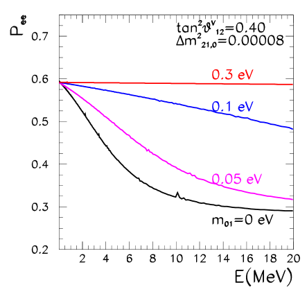
Figure 29: Survival probability of solar $\nu_{e}$’s as a function of the neutrino energy. This survival probability has been obtained for neutrinos produced around $x=0.05$ as it is characteristic of ${}^{8}\text{B}$ neutrinos.

The $\nu_{e}$ survival probability is obtained by solving numerically the evolution equation. In most of the parameter space the evolution of the neutrino system is adiabatic and the survival probability is well reproduced by the standard formula, Eq. (76), with an effective mixing angle in matter at the neutrino production point $x_{0}$, $\theta^{m}_{12,0}$. It includes both the effect of the point dependent kinetic mass splitting as well as the effect of the MSW potential $V_{e}(x)$

$$\cos 2\theta^{m}_{12,0}=\frac{\Delta m^{2}_{\text{kin}}(x_{0})\cos 2\theta_{12}-A(x_{0})}{\sqrt{[\Delta m^{2}_{\text{kin}}(x_{0})\cos 2\theta_{12}-A(x_{0})]^{2}+[\Delta m^{2}_{\text{kin}}(x_{0})\sin 2\theta_{12}]^{2}}}$$ (228)

where $A(x_{0})=2EV_{e}(x_{0})$. In Fig. 29 the survival probability is plotted for different values of the neutrino mass scale $m_{01}$. As can be seen in the figure, due to the different contributions of the solar neutrino background to the two mass eigenstates, the energy dependence of the survival probability is rapidly damped even for mildly degenerated neutrinos. As a consequence, in these cases, it is not possible to simultaneously accommodate the observed event rates in solar neutrino experiments and in KamLAND as shown in Fig. 30.

Figure 30: Allowed regions from the global analysis of solar and solar plus KamLAND data in the $(\Delta m^{2}_{21,0},\tan^{2}\theta_{12},m_{01})$ parameter space, shown for 4 sections at fixed values of $m_{01}$. The different contours corresponds to 90%, 95%, 99%, and 3$\sigma$ CL for 3 d.o.f. The global minima are marked with a star.

6.2 Mass Varying Neutrinos in the Sun: Matter Density Effects

In principle it is possible that the acceleron couples not only to the neutrinos but also to the visible matter. Such coupling would be induced by non-renormalizable operators and it would imply that neutrino masses depend on the visible matter background density as well. This matter background dependence could lead to interesting phenomenological consequences for neutrino oscillations [224, 234, 235, 236].

Generically one can parametrize these effects in an effective low energy model containing the Standard Model particles plus a light scalar ($\phi$) of mass $m_{S}$ which couples very weakly both to neutrinos ($\nu_{i}$) and the matter fields $f=e,n,p$:

$$\mathcal{L}=\sum_{i}\bar{\nu}_{i}\left(i/\!\!\!\partial-m_{0i}\right)\nu_{i}+\sum_{f}\bar{f}\left(i/\!\!\!\partial-m^{0}_{f}\right)f+\frac{1}{2}\left[\phi\left(\partial^{2}-m_{S}^{2}\right)\phi\right]\\ +\sum_{ij}\lambda^{\nu}_{ij}\bar{\nu}_{i}\nu_{j}\phi+\sum_{f}\lambda^{f}\bar{f}f\phi\,,$$ (229)

$\lambda^{\nu}_{ij}$ and $\lambda^{f}$ are, respectively, the effective neutrino-scalar and matter-scalar couplings.

In the context of the dark energy-related MaVaNs models of Ref [222, 223, 224] discussed in the previous section the scalar $\phi$ would be the acceleron – with mass in the range $m_{S}\sim 10^{-6}$–$10^{-8}$ eV – which, when acquiring a non-vanishing expectation value, $\langle\phi\rangle$, gives a contribution to the neutrino mass. This in turn implies that the acceleron effective potential receives a contribution which changes as a function of the neutrino density, so that

$$\lambda^{\nu}=\left.\frac{\partial m_{\nu}}{\partial\phi}\right|_{\langle\phi\rangle}\,.$$ (230)

$\lambda^{f}$, the effective low energy couplings of the acceleron to visible matter, come from non-renormalizable operators which couple the acceleron to the visible matter, such as might arise from quantum gravity. They are constrained by tests of the gravitational inverse square law (ISL) which require [237]

$$\lambda^{n},\lambda^{p}\lesssim 10^{-21}$$ (231)

for any scalar with $m_{S}\gtrsim 10^{-11}$ eV.

Eq. (229) implies that in a medium with some additional neutrino background (either relativistic or non-relativistic) as well as non-relativistic matter (electrons, protons and neutrons), neutrinos acquire masses which obey the following set of integral equations

$$m_{ij}(x) =m_{0i}\delta_{ij}-M_{ij}(x),$$ (232)

$$M_{ij}(x) =\frac{\lambda^{\nu}_{ij}}{m_{S}^{2}}\left(\sum_{f}\lambda^{f}n_{f}(x)+\sum_{a}\lambda^{\nu}_{aa}\int\frac{d^{3}k}{(2\pi)^{3}}\,\frac{M_{aa}}{\sqrt{k^{2}+M_{aa}^{2}}}\,f_{a}(r,k)\right).$$

$n_{f}(x)$ is the number density for the fermion $f$, and $f_{a}(x,k)$ is the sum of neutrino and antineutrino “$a$” occupation numbers for momentum $k$ in addition to the cosmic background neutrinos.

The results in Eq. (230) and Eq. (232) correspond to the first order term in the Taylor expansion around the present epoch background value of $\phi$. In general, for the required flat potentials in these models, one needs to go beyond first order and the neutrino mass is not linearly proportional to the number density of the particles in the background as shown in Sec. 6.1. The exact dependence on the background densities is function of the specific form assumed for the scalar potential. This is mostly relevant for the neutrino density contribution to the neutrino mass, while for small enough couplings to the matter potential one expects the linear approximation to hold better.

As seen in the previous section for solar neutrinos the neutrino background contribution is only relevant as long as the neutrinos are not very hierarchical. On the other hand for solar neutrinos of hierarchical masses ($m_{01}\simeq 0$) the dominant contribution to the neutrino mass is due to the matter background density. In this section we will describe the phenomenology of solar and KamLAND neutrinos in this scenario for which

$$M_{ij}(x)=\frac{\lambda^{\nu}_{ij}}{m_{S}^{2}}\sum_{f}\lambda^{f}n_{f}(x)\,.$$ (233)

6.2.1 Effects on Solar Neutrinos and KamLAND

Assuming that the oscillation of solar and reactor antineutrinos are still dominated by a single mass scale even in the presence of these effects one can parametrize their evolution equation Eq. (205) with

$$M^{2}(x)=\begin{pmatrix}M_{1}^{2}(x)&M_{3}^{2}(x)\\ M_{3}^{2}(x)&[m_{02}-M_{2}(x)]^{2}\end{pmatrix}\quad\text{and}\quad V(x)=\begin{pmatrix}V_{e}(x)&~{}0\\ 0&~{}0\end{pmatrix}\,,$$ (234)

where $M_{i}(r)$ are the ED contributions to the neutrino masses Eq. (233).

In general, for given matter density profiles, Eq. (205) has to be solved numerically. But in most of the parameter space allowed by KamLAND and solar data the transition is adiabatic and the survival probability is well reproduced by the standard formula, Eq. (76), with an effective mixing angle in matter at the neutrino production point $x_{0}$, $\theta^{m}_{12,0}$:

$$\cos 2\theta^{m}_{12,0}=\frac{(\Delta\tilde{M}_{21}^{2}(x_{0})\cos 2\tilde{\theta}_{12,0}-2EV_{e}(x_{0}))}{\sqrt{[\Delta\tilde{M}_{21}^{2}(x_{0})\cos 2\tilde{\theta}_{12,0}-2EV_{e}(x_{0})]^{2}+[\Delta\tilde{M}_{21}^{2}(x_{0})\sin 2\tilde{\theta}_{12,0}]^{2}}}\,,$$ (235)

with

$$\Delta\tilde{M}_{21}^{2}(x_{0})=2\sqrt{M_{3}^{4}(x_{0})+\left(\frac{\Delta M^{2}_{21}(x_{0})}{2}\right)^{2}}$$ (236)

$$\cos 2\tilde{\theta}_{12,0}=\frac{\dfrac{\Delta M_{21}^{2}(x_{0})}{2}\cos 2\theta_{21}-M_{3}^{2}(x_{0})\sin 2\theta_{12}}{\sqrt{M_{3}^{4}(x_{0})+\left(\dfrac{\Delta M^{2}_{21}(x_{0})}{2}\right)^{2}}}$$ (237)

and where

$$\Delta M^{2}_{21}(x_{0})=[m_{02}-M_{2}(x_{0})]^{2}-M_{1}^{2}(x_{0})\,.$$ (238)

As discussed above, in general, $M_{i}(r)$ can be an arbitrary function of the background matter density. In the linear approximation given in Eq. (233) and for $\lambda^{e}\ll\lambda^{n}=\lambda^{p}\equiv\lambda^{N}$, these terms can be parametrized as:

$$M_{i}(x)=\alpha_{i}\,\left[\frac{\rho(x)}{\text{gr}/\text{cm}^{3}}\right]\,,$$ (239)

where $\rho$ is the matter density, and the characteristic value of the $\alpha$ coefficients is

$$\alpha\sim 4.8\times 10^{23}\,\lambda^{\nu}\,\lambda^{N}\,\left(\frac{10^{-7}\text{eV}}{m_{S}}\right)^{2}\,\text{eV}\,.$$ (240)

One must notice, however, that, as long as the transition is adiabatic, the survival probability only depends on the value of $M_{i}(x)$ at the neutrino production point. Therefore it only depends on the exact functional form of $M_{i}(x)$ via the averaging over the neutrino production point distributions.

The survival probability for anti-neutrinos, $P_{\bar{e}\bar{e}}$, which is relevant for KamLAND, takes the form

$$P_{\bar{e}\bar{e}}=1-\sin^{2}2\theta^{m}_{12,0}\,\sin^{2}\left(\frac{\Delta m^{2}_{KL}L}{2E}\right)\,,$$ (241)

where $\cos 2\theta^{m}_{12,0}$ is defined as in Eq. (235) and $\Delta m^{2}_{KL}$ is the denominator of this equation but replacing $V_{e}$ by $-V_{e}$ and assuming a constant matter density $\rho\sim 3$ gr/cm³, typical of the Earth’s crust.

To illustrate the expected size of the effect we show in Fig. 31 the evolution of the mass eigenstates $m_{1}$ and $m_{2}$ in matter as a function of $V_{e}E$ for different values of $\alpha_{2}$ (keeping $\alpha_{1}=\alpha_{3}=0$). As a reference, we also show in this figure the standard MSW evolution curve (solid line) for the oscillation parameters at $\Delta m^{2}_{0,21}=(m_{02})^{2}=8\times 10^{-5}~{}\text{eV}^{2}$ and $\tan^{2}\theta_{12}=0.4$. From this plot we can appreciate that in the region relevant to solar neutrino experiments the evolution of the mass eigenstates is not significantly different from the MSW one if $|\alpha_{2}|\lesssim 10^{-5}$ eV. For larger values of $\alpha_{2}$, such as $|\alpha_{2}|=10^{-4}$ eV, we expect solar neutrinos to be affected. On the other hand, KamLAND data is very little affected by the ED terms in this range of $\alpha_{2}$.

Fig. 31 also illustrates a curious feature of these scenarios: the fact that it is possible to find a value of the matter dependence term which exactly cancels $\Delta m^{2}_{0,21}$. It can be seen, directly from Eqs. (205), that if for a particular point, $r_{0}$, in the medium, $m_{02}=M_{2}(r_{0})$ and $M_{1}=M_{3}=0$ ($\alpha_{1}=\alpha_{3}=0$) the lower mass eigenstate will be zero while the higher one will be at the corresponding value of $2V_{e}(r_{0})E$.

Non-adiabatic effects in the Sun can also occur. In the region of relatively small $\alpha$ parameters, non-adiabaticity occurs when the parameters are “tuned” to give a vanishing effective $\Delta m^{2}_{21}$ (the denominator of Eq. (235)). This can be achieved, for example, with $\alpha_{1}=\alpha_{2}=0$ by solving the following set of equations inside the Sun:

$$(m_{02})^{2}\cos 2\theta-2M^{2}_{3}(x)\sin 2\theta =2EV_{e}(x),$$ (242)

$$(m_{02})^{2}\sin 2\theta+2M^{2}_{3}(x)\cos 2\theta =0.$$ (243)

It can be shown that for $\alpha_{3}=i\,5.5\times 10^{-5}$ eV, $\tan^{2}\theta=0.3$ and $E=10$ MeV this set of equations are fulfilled at $r/R_{\odot}\sim 0.027$, and the neutrinos would suffer a non-adiabatic transition on their way out of the Sun. However, in general for the small values of the $\alpha$ parameters discussed here, these non-adiabatic effects do not lead to a better description of the solar neutrino data.

More generically, non-adiabatic effects occur for sufficiently large values of the $\alpha$ parameters so that one can disregard the standard MSW potential $V_{e}$ and the vacuum mass $m_{02}$ with respect to the matter density mass dependent terms. In this case, as seen from Eq. (235), the mixing angle inside the Sun is constant and controlled by the $\alpha^{\prime}s$. At the border of the Sun, as the density goes to zero, the mixing angle is driven to its vacuum value in a strongly non-adiabatic transition. This scenario would be equivalent to a vacuum-like oscillation for solar neutrinos with the ED of neutrino mass having to play a leading role in the interpretation of terrestrial neutrino experiments. Given the strong constraints from atmospheric neutrino experiments on new physics scenarios described in Sec. 5, it is difficult to foresee that this scenario could lead to a successful global description of the oscillation data.

Figure 31: Evolution of the neutrino mass eigenstates in matter with $m_{02}^{2}=8\times 10^{-5}~{}\text{eV}^{2}$, $\tan^{2}\theta_{12}=0.4$ and different values of the ED parameters as labeled. The solid lines represent the standard MSW evolution. The shaded regions correspond to typical values of $V_{C}C\equiv V_{e}$ in neutrino production region in the center of the Sun for the Solar $\nu$’s region, and a constant Earth crust density of 3 g/cm³, with a proton density fraction of $Y=0.5$ and neutrino energies varying from 3 to 10 MeV for the KamLAND region.

Altogether it is found that for specific values of the ED couplings some modification of the allowed $\Delta m^{2}$ regions are possible. For example in Ref. [235] it was shown that the presence of these effects can improve the agreement with solar neutrino data within the LMA region while being perfectly consistent with KamLAND data. In Ref. [236] it was also found that the description of the solar data in the high-$\Delta m^{2}$ KamLAND region can be significantly improved and there is a new allowed solution in the global solar plus KamLAND analysis at the 98.9% CL around $\tan^{2}\theta_{12}=0.5$ and $\Delta m^{2}_{0,21}=1.75\times 10^{-4}~{}\text{eV}^{2}$. We show in Fig. 32 the survival probability for this best fit point in that high-$\Delta m^{2}$ region in the presence of ED effects. This solution will be further tested by a more precise determination of the antineutrino spectrum in KamLAND. In particular with an improvement of the systematic error down to 4% and an accumulated statistics of 3Kt-years, the LMAI solution could be ruled out beyond 3$\sigma$ [242].

Figure 32: $\nu_{e}$ survival probability in the Sun versus neutrino energy for the best fit point in the high-$\Delta m^{2}$ region in the presence of ED effects. The dotted line is the survival probability for conventional oscillations ($\alpha_{i}=0$) with the same values of $\Delta m^{2}_{21,0}$ and $\theta_{12}$. These survival probabilities have been obtained for neutrinos produced around $x=0.05$ as it is characteristic of ${}^{8}\text{B}$ and ${}^{7}\text{Be}$ neutrinos. The data points are the extracted average survival probabilities for the low energy ($pp$), intermediate energy (${}^{7}\text{Be}$, $pep$ and CNO) and high energy solar neutrinos (${}^{8}\text{B}$ and $hep$) from Ref. [235].

More generically, the global analysis of solar and KamLAND data can be used to constraint the possible size of the ED contribution to the neutrino mass and correspondingly of the possible size of the acceleron couplings to matter and neutrinos. This is illustrated in Fig. 33 where we show the result of such global analysis in the form of the allowed two-dimensional regions in the $(\alpha_{2},\alpha_{3})$ (for $\alpha_{1}=0$) parameter space after marginalization over $\Delta m^{2}_{0,21}$ and $\tan^{2}\theta_{12}$.

Figure 33: Allowed regions from the global analysis of solar and solar plus KamLAND data in the $(\alpha_{2},\alpha_{3})$ parameter space. The curves correspond to 1$\sigma$, 90%, 95%, 99% and $3\sigma$ CL (2 d.o.f.). The best fit point at $\alpha_{2}=10^{-4}$ eV and $\alpha_{3}=i\,2.0\times 10^{-5}$ eV, represented by a star, is also shown.

From the combined analysis one can derive the following 3 $\sigma$, bounds (with 1 d.o.f.)

$$\begin{gathered}-5.6\times 10^{-5}\leq\alpha_{2}/\text{eV}\leq 1.7\times 10^{-4}\,,\\ |\alpha_{3}|/\text{eV}\leq\begin{cases}8\times 10^{-5}&\text{for}\quad\alpha_{3}^{2}>0\,,\\ 5\times 10^{-5}&\text{for}\quad\alpha_{3}^{2}<0\,.\end{cases}\end{gathered}$$ (244)

These bounds can be converted into a limit on the product of the characteristic effective neutrino-scalar and matter-scalar couplings. For example, at 90% CL,

$$|\lambda^{\nu}\,\lambda^{N}|\,\left(\frac{10^{-7}\,\text{eV}}{m_{S}}\right)^{2}\leq 3.0\times 10^{-28}\,.$$ (245)

This bound can be compared to those derived from tests of the ISL, Eq. (231). We conclude that if the scalar also couples to neutrinos with coupling

$$\lambda^{\nu}\gtrsim 3.0\times 10^{-7}\left(\frac{m_{S}}{10^{-7}\,\text{eV}}\right)^{2}\,,$$ (246)

the analysis of solar and KamLAND data yields a more restrictive constraint on the matter-scalar couplings than ISL tests.

6.3 Leptonic Long Range Forces

We now turn to the possible effects arising from long range forces coupling to flavor symmetries. Since the seminal work of Lee and Yang [225] it has become standard to consider long-range forces coupling to baryon and/or lepton number. These forces violate the universality of free fall and thus they can be tested by Eötvös-type experiments, as pointed out in [225, 243, 244, 245]. At present such tests yield a bound the “fine structure” constant of a vector force associated to $L$:

$$k_{V}<10^{-49}\,.$$ (247)

Since neutrinos are massive the lepton flavor symmetries $L_{i}$ ($i=e,\,\mu,\,\tau$) cannot be exact in nature. Thus if an electronic (or muonic, taunic) force exists, we may expect it to be of arbitrary but finite range. When the range of the force is less than the Earth-Sun distance, the bound (247) is no longer valid. Other experiments [246, 237] using the Earth as electronic source instead of using the Sun place bounds, which however are much less strict than (247).

Neutrino oscillations are sensitive probes to such forces. If there is a new force coupled to the leptonic flavor numbers, its presence will affect neutrino oscillations when neutrinos travel through regions where a flavor dependent density of leptons is present. As discussed in Ref. [247] the effect of the new interaction on the oscillation pattern depends on its Lorentz structure. Nevertheless, as we will show below for scalar, vector or tensor interactions of large enough range the modification of the evolution equation can always be casted in terms of a unique function which solely depends on the background density of leptons – the source of the force – and the range of the interaction.

In this form, in Ref. [248] it was discussed that atmospheric neutrino data can constrain the strength of vector forces coupled to $L_{e}-L_{\mu}$, $k_{V}(e\mu)\leq 5.5\times 10^{-52}$, and to $L_{e}-L_{\tau}$, $k_{V}(e\tau)\leq 6.4\times 10^{-52}$ (at 90% CL) when the range of the force is the Earth-Sun distance. Also, new vector forces coupling individually to muonic or tauonic number can be constrained, giving however worse bounds. For example, primordial nucleosynthesis considerations provide the bound $k_{V}(\mu,\tau)<1.8\times 10^{-11}$ [249].

Because of the larger electron density in the solar environment stronger effects are expected in solar neutrino observables [250, 247, 251]. If the new interaction is flavor diagonal its effect in the evolution of atmospheric neutrinos does not modify the hierarchy (93) and the 2$\nu$ oscillation factorization still holds. In this case in general, one can write the solar neutrino evolution equation in the presence of the new force as Eq. (205) where both ${M}(x)$ and $V(x)$ depend on the Lorentz structure of the leptonic interaction as follows:

• Let’s start studying the case in which the new force is mediated by a neutral vector boson $A_{\alpha}$ with a small finite mass $m$ so that the new contribution to the Lagrangian is:

  $$\mathcal{L}=-g_{1}A_{\alpha}\bar{\psi}_{\nu}\gamma^{\alpha}\psi_{\nu}-g_{1}A_{\alpha}\bar{\psi}_{e}\gamma^{\alpha}\psi_{e}\,.$$ (248)

  The electrons in the Sun can be thought as the source of a solar leptonic field, described by the external static classical vector potential

  $$A_{\mu}^{ext}(\vec{r})\equiv\frac{1}{\sqrt{(2\pi})^{3}}\int d^{3}k\,e^{i\vec{k}\vec{r}}\,\tilde{A}_{\mu}^{ext}(\vec{k})\,,$$ (249)

  with

  $$\tilde{A}_{\mu}^{ext}(\vec{k})=-\frac{1}{k^{2}-m^{2}}\,g_{1}\,\tilde{j}^{e}_{\mu}(k)\,,$$ (250)

  where $k^{2}=-|\vec{k}|^{2}$ and

  $$\tilde{j}^{e}_{\mu}(k)=\frac{1}{\sqrt{(2\pi})^{3}}\,\int d^{3}\rho\,e^{-i\vec{k}\vec{\rho}}\,\bar{\psi}_{e}(\vec{\rho})\gamma_{\mu}\psi_{e}(\vec{\rho})\,,$$ (251)

  In the NR limit one can neglect the spatial components of the current and the only non-vanishing piece is:

  $$\tilde{j}^{e}_{0}(k)=\frac{1}{\sqrt{(2\pi})^{3}}\int d^{3}\rho\,e^{-i\vec{k}\vec{\rho}}\,\bar{\psi}_{e}(\vec{\rho})\gamma_{0}\psi_{e}(\vec{\rho})=\frac{1}{\sqrt{(2\pi})^{3}}\int d^{3}\rho\,e^{-i\vec{k}\vec{\rho}}\,n_{e}(\vec{\rho})\,.$$ (252)

  $n_{e}(\vec{\rho})$ is the electron number density. Thus the only non-vanishing component of the vector potential is

  $$A_{0}^{ext}(\vec{r}) =\frac{g_{1}}{(2\pi)^{3}}\int\d^{3}\rho\,n_{e}(\rho)\int d^{3}k\,e^{i\vec{k}(\vec{r}-\vec{\rho})}\,\frac{1}{|\vec{k}|^{2}+m^{2}}$$ (253)

  $$=\frac{g_{1}}{4\pi}\,\int\d^{3}\rho\,n_{e}(\vec{\rho})\,\frac{e^{-|\vec{\rho}-\vec{r}|/\lambda}}{|\vec{\rho}-\vec{r}|}$$

  where $\lambda=1/m$. Introducing this result in Eq. (248) we get a contribution to the Lagrangian for the neutrinos of the form

  $$-\frac{g_{1}^{2}}{4\pi}\int\d^{3}\rho\,n_{e}(\vec{\rho})\,\frac{e^{-|\vec{\rho}-\vec{r}|/\lambda}}{|\vec{\rho}-\vec{r}|}\,\bar{\psi}_{\nu}\gamma^{0}\psi_{\nu}\,,$$ (254)

  which can be interpreted as a contribution to the potential energy for the neutrinos $V(r)=k_{V}(e)W(r)$ with $k_{V}(e)=\dfrac{g_{1}^{2}}{4\pi}$ and

  $$\begin{split}W(r)&=\int\frac{e^{-|\vec{\rho}-\vec{r}|/\lambda}}{|\vec{\rho}-\vec{r}|}\,d^{3}\rho\\ &=\frac{2\pi\lambda}{r}\int_{0}^{R_{\text{Sun}}}n_{e}(\rho)\,\rho\left[e^{-|\rho-r|/\lambda}-e^{-(\rho+r)/\lambda}\right]\,d\rho\end{split}$$ (255)

  where $R_{\odot}$ is the radius of the Sun, $n_{e}(r)$ is the electron number density in the medium (assumed here to be spherically symmetric) and $\lambda$ is the range of the interaction. In summary we can write the solar neutrino evolution equation in the presence of the new force as Eq. (205) where

  $$M_{ij}=m_{0i}\,\delta_{ij}\quad\text{and}\quad V(x)=V_{e}(x)+k_{V}(e)\,W(r)$$ (256)

  with $k_{V}(e)=\dfrac{g_{1}^{2}}{4\pi}$. As a consequence of the vector structure of the force, the new leptonic potential adds to the MSW potential with the same energy dependence and sign. It will accordingly flip sign when describing antineutrino oscillations.

• In the same fashion one can show that if the new force is mediated by a neutral spin $J=0$ particle, $\phi$, so that the new contribution to the Lagrangian reads:

  $$\mathcal{L}=-g_{0}\phi\bar{\psi}_{\nu}\psi_{\nu}-g_{0}\phi\bar{\psi}_{e}\psi_{e}$$ (257)

  the corresponding external scalar “potential” due to the solar electrons is:

  $$\phi^{ext}(r)=-\frac{g_{0}}{4\pi}\,W(r)\,,$$ (258)

  which gives a contribution to the Lagrangian for the neutrinos of the form

  $$\frac{g_{0}^{2}}{4\pi}\,W(r)\,\bar{\psi}_{\nu}\psi_{\nu}\,,$$ (259)

  which can be interpreted as a contribution to the effective $\nu_{e}$ mass. So the solar neutrino evolution equation in the presence of the new force takes the form Eq. (205) where now

  $$M=\begin{pmatrix}m_{01}&0\\ 0&m_{02}\end{pmatrix}-U_{12}^{\dagger}\,\begin{pmatrix}k_{S}(e)\,W(x)&~{}0\\ 0&~{}0\end{pmatrix}\,U_{12}\quad\text{and}\quad V(r)=V_{e}(x)\,.$$ (260)

  $k_{S}(e)=\dfrac{g_{0}^{2}}{4\pi}$ and the $k_{S}(e)\,W(x)$ term has the same sign for neutrinos and antineutrinos. $m_{0i}$ are the neutrino masses in vacuum.

• Similarly for a $L_{e}$-coupled force mediated by a tensor field of spin $J=2$, $\chi_{\alpha\beta}$:

  $$\mathcal{L}=-g_{2}\,\chi_{\alpha\beta}T^{\alpha\beta}_{\nu}-g_{2}\,\chi_{\alpha\beta}T^{\alpha\beta}_{e}$$ (261)

  where $T^{\alpha\beta}$ is the energy-momentum tensor for either electrons or neutrinos:

  $$T^{\alpha\beta}=\left[\bar{\psi}\gamma^{\alpha}i\partial^{\beta}\psi-i\partial^{\alpha}\bar{\psi}\gamma^{\beta}\psi\right]\,.$$ (262)

  The solar electrons can be the source of an static tensor field whose only non-vanishing contributions are:

  $$\chi^{ext}_{00}(r)=\chi^{ext}_{ii}(r)=-g_{2}\,m_{e}\frac{1}{4\pi}\,W(r)\,,$$ (263)

  where $m_{e}$ is the mass of the electron. The action of this potential on the neutrinos is

  $$-m_{e}\,\frac{g_{e}^{2}}{4\pi}\,W(r)\,(T^{00}_{n}u\,+\,\sum_{i}T^{ii}_{\nu})=-m_{e}\,E\,\frac{g_{e}^{2}}{4\pi}\,W(r)\,\bar{\psi}_{\nu}\gamma^{0}\psi_{\nu}\,,$$ (264)

  where in the last line we have used the Dirac equation for a massless neutrino of energy $E$ (introducing the neutrino mass here leads to a higher order correction on the neutrino evolution equation). This can be interpreted as a contribution to the neutrino potential so that the neutrino evolution equation takes the form Eq. (205) with

  $$M_{ij}=m_{0i}\,\delta_{ij}\quad\text{and}\quad V(x)=V_{e}(x)-Ek_{T}(e)W(x)\,.$$ (265)

  $k_{T}(e)=m_{e}\dfrac{g_{2}^{2}}{4\pi}$ (notice that the coupling constant $g_{2}$ has dimensions $1/E$). As for the case of a scalar leptonic force, the tensor force is always symmetric when changing from neutrinos to antineutrinos. This is so because what couples to the tensor field $\chi$ is in fact the energy momentum tensor of the leptons which has to be symmetric under the exchange of particles and antiparticles.

We see that for all cases one can define the universal function $W$ as Eq.(255) determining the effect of the force coupled to $L_{e}$ at a point $r$ from the center of the Sun. In Fig. 34 we show the function $W(x)$ in the Sun as a function of the distance in units of $R_{\odot}$ for various ranges $\lambda$.

Figure 34: Leptonic potential function $W(r)$ due to the density of electron in the Sun as a function of the distance from the solar center in units of $R_{\odot}$ for various ranges $\lambda$.

For the range of parameters of interest the evolution in the Sun and from the Sun to the Earth is always adiabatic. The energy dependence of the resulting survival probability of solar $\nu_{e}$ at the sunny face of the Earth is shown in Fig. 35. From this figure we see that for $m_{1}=0$, values of $k_{S}(e)\gtrsim 10^{-45}$–$10^{-44}$ will conflict with the existing solar neutrino data while for $m_{1}=0.1$ eV even smaller values of the coupling, $k_{S}(e)\lesssim 10^{-46}$–$10^{-45}$, will be rule out. In the third panel we show the vector case for some values of $k_{V}(e)$. One expects from this that our analysis will lead to bounds $k_{V}(e)\lesssim 10^{-54}$–$10^{-53}$. Finally, in the lower panel the tensor case is displayed. In this case one expects that the data will constrain $k_{T}(e)\lesssim 10^{-61}$–$10^{-60}$ eV^-1.

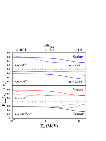
Figure 35: Survival probability of $\nu_{e}$ in the Sun as a function of the neutrino energy $E$ for an infinite range scalar (first two panels), vector (third panel) and tensor (lower panel) leptonic force, for various values of the strength and range. For all curves $\tan^{2}\theta_{12}=0.44$ and $\Delta m^{2}_{21}=7.9\times 10^{-5}~{}\text{eV}^{2}$.

More quantitatively in Ref. [247] it was shown that the combined analysis of solar and KamLAND data provides the following bounds for infinite range $\lambda=\infty$

$$k_{S} \leq 5\times 10^{-45}$$ (266)

$$k_{V} \leq 2.5\times 10^{-53}$$ (267)

$$k_{T} \leq 1.7\times 10^{-60}~{}\text{eV}^{-1}$$ (268)

at $3\sigma$ (1 d.o.f.). These bounds are practically the same for any $\lambda\gtrsim 10\,R_{\text{Sun}}$. For $\lambda\lesssim 10\,R_{\text{Sun}}$, the bound slowly worsens, and for $\lambda\sim 0.1\,R_{\text{Sun}}$ we have that the bound on $k_{i}$ is a factor less than 10 worse than (266)–(268) as illustrated in Fig. 36.

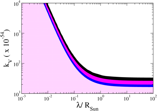
Figure 36: Allowed regions from the global analysis of solar plus KamLAND data in the $(k_{V},\lambda/R_{\text{Sun}})$ at 90%, 95%, 99% and 3$\sigma$ CL (2 d.o.f.) for a leptonic vector force.

In some cases these effects can also modify the allowed ranges of $\Delta m^{2}$ for specific values of the couplings. In particular in the presence of scalar forces for highly hierarchical neutrinos and $4.5\leq k_{S}(e)/10^{-45}\leq 8$ and/or vector forces with $2\leq k_{V}(e)/10^{-54}\leq 30$ the description of the solar data in the high-$\Delta m^{2}$ region of KamLAND can be significantly improved and there is a new allowed solution at the 98.9% CL around $\tan^{2}\theta_{12}=0.5$ and $\Delta m^{2}_{0,21}=1.7\times 10^{-4}~{}\text{eV}^{2}$ [247].

6.4 Neutrino Magnetic Moment

Non-zero neutrino masses can manifest themselves also through non-standard neutrino electromagnetic properties. For example, if the lepton sector in the Standard Model is minimally extended in analogy with the quark sector, neutrinos get Dirac masses ($m_{\nu}$) and their magnetic moments (MMs) are tiny [252],

$$\mu_{\nu}\simeq 3\times 10^{-19}~{}\mu_{B}\left(\frac{m_{\nu}}{1~{}\text{eV}}\right)\,,$$ (269)

where $\mu_{B}$ is the Bohr magneton.

In general models, however, there is no such direct proportionality between the neutrino mass and its coupling to the electromagnetic interactions. Consequently neutrinos can have sizable magnetic moment and/or electric dipole moment (EDM) couplings which can show a non-trivial flavor structure. Thus the existence of any electromagnetic neutrino moment well above the expectation in Eq. (269) would signal that some special mechanism—which goes beyond the SM—is at work. Therefore, neutrino electromagnetic properties are interesting probes of new physics.

In the flavor basis the interaction of Dirac neutrinos with a MM and an EDM with the electromagnetic field is described by the Hamiltonian

$$H_{\text{em}}^{D}=\frac{1}{2}\bar{\nu}_{R}\lambda\sigma^{\alpha\beta}\nu_{L}F_{\alpha\beta}+\text{h.c.}$$ (270)

Here $\nu^{T}_{L(R)}=(\nu_{e},\,\nu_{\mu},\,\nu_{\tau},\,\nu_{s},\,\ldots)_{L(R)}$ is the vector of the left-handed (right-handed) flavor eigenfields including an arbitrary number of sterile neutrinos. The hermitian matrices $\mu$ of MMs and $d$ of EDMs are condensed in the non-hermitian matrix

$$\lambda=\mu-id\quad\text{with}\quad\mu=\frac{\lambda+\lambda^{\dagger}}{2}\,,\quad d=\frac{i(\lambda-\lambda^{\dagger})}{2}\,.$$ (271)

In the mass basis, Eq.(20), the matrix (271) transforms as

$$\tilde{\lambda}={V^{\nu}_{R}}^{\dagger}\lambda V^{\nu}\,.$$ (272)

Similarly, for Majorana neutrinos:

$$H_{\text{em}}^{M}=-\frac{1}{4}\nu_{L}^{T}C^{-1}\lambda\sigma^{\alpha\beta}\nu_{L}F_{\alpha\beta}+\text{h.c.}\,,$$ (273)

where $C$ is the charge conjugation matrix. For Majorana neutrinos CPT conservation implies that the matrix $\lambda$, defined as in Eq. (271), is antisymmetric and correspondingly the MM and EDM matrices are antisymmetric and hermitian [32]. In the mass basis of the Majorana neutrino fields

$$\tilde{\lambda}={V^{\nu}}^{T}\lambda V^{\nu}\,.$$ (274)

Neutrino MM and EDM’s can be searched for by detecting their effect in the neutrino-electron scattering cross section. In the SM, neutrinos interact with electrons only via weak currents. But a neutrino MM and/or EDM adds an extra component due to photon exchange [253, 254]. For a neutrino produced in a source with flavor $\beta$, $\nu_{\beta}$, this additional contribution reads:

$$\frac{d\sigma_{\text{em}}}{dT}=\frac{\alpha^{2}\pi}{m_{e}^{2}\,\mu_{B}^{2}}\left(\frac{1}{T}-\frac{1}{E_{\nu}}\right)\mu^{2}_{\text{eff}}(\nu_{\beta})\,.$$ (275)

Here $T$ denotes the kinetic energy of the recoil electron, $E_{\nu}$ is the energy of the incoming neutrino. The effective MM square is given by [255]

$$\mu^{2}_{\text{eff}}(\nu_{\beta})=a_{\beta-}^{\dagger}\lambda^{\dagger}\lambda a_{\beta-}+a_{\beta+}^{\dagger}\lambda\lambda^{\dagger}a_{\beta+}\,.$$ (276)

The vectors $a_{\beta\pm}$ denote the neutrino amplitudes for negative and positive helicities, respectively, at the detector after propagation, so that the state arriving in the detector is:

$$|\nu\rangle_{\text{det}}=\sum_{\alpha=e,\mu,\tau,s,\ldots}\left(a_{\beta-}^{\alpha}|\nu^{(-)}_{\alpha}\rangle+a_{\beta+}^{\alpha}|\nu^{(+)}_{\alpha}\rangle\right)\,.$$ (277)

In the massless limit the negative helicity states are left-handed neutrinos whereas the positive helicity states are sterile right-handed neutrinos in the Dirac case and right-handed antineutrinos in the Majorana case. In general, for neutrinos coming from distance sources, these amplitudes depend on the initial neutrino flavor, its energy and the distance between source and detector and are obtained by solving the neutrino evolution equation as described below.

The electromagnetic cross section adds to the weak cross section and allows to extract information on the TM matrix $\lambda$. In this respect it is important to notice that the square of the effective MM given in Eq. (276) is independent of the basis chosen [255] and it only depends on the neutrino flavor at the source and on its propagation.

At laboratory experiments with terrestrial baselines the vectors $a_{\beta\pm}$ are simply unity vectors pointing on the corresponding neutrino ($-$) (or antineutrino $(+)$) flavor direction, since in those experiments the baseline is much too short for any oscillations to develop and then $|\nu\rangle_{\text{det}}=|\nu_{\beta}\rangle$. For example, for a reactor neutrino experiment the source is $\bar{\nu}_{e}$ and we have $a_{\beta-}=a_{e-}-=0$ and $a_{\beta+}=a_{e+}=(1,\,0,\,0)^{T}$.

At present, laboratory experiments give 90% CL bounds on the neutrino magnetic moments of $1.9\times 10^{-10}~{}\mu_{B}$ [256], $9\times 10^{-11}~{}\mu_{B}$ [257], $7.4\times 10^{-11}~{}\mu_{B}$ [258] and $5.8\times 10^{-11}~{}\mu_{B}$ [259] for the electron neutrino, $6.8\times 10^{-10}~{}\mu_{B}$ for the muon neutrino [109] and $3.9\times 10^{-7}~{}\mu_{B}$ for the tau neutrino [260] (see also Ref. [23]). On the other hand, astrophysics and cosmology provide limits of the order of $10^{-12}$ to $10^{-11}$ Bohr magnetons [261]. Improved sensitivity for the electron neutrino MM from reactor neutrino experiments is expected, while experiments with tritium sources aims to reach $10^{-12}~{}\mu_{B}$ [262, 263].

For solar neutrino phenomenology it was also important the realization that the existence of magnetic transition (flavor non-diagonal) moments (TM) leads to the phenomenon of spin-flavor precession (SFP) [32, 264], when they move through a magnetic field, as might happen in the Sun. In this case their evolution equation is (we follow the notation of Ref. [255]):

$$i\frac{d}{dz}\begin{pmatrix}\varphi_{-}\\ \varphi_{+}\end{pmatrix}=\begin{pmatrix}V_{L}+\frac{1}{2E}M_{\nu}^{\dagger}M_{\nu}&-B_{+}\lambda^{\dagger}\\ -B_{-}\lambda&V_{R}+\frac{1}{2E}M_{\nu}M_{\nu}^{\dagger}\end{pmatrix}\begin{pmatrix}\varphi_{-}\\ \varphi_{+}\end{pmatrix}\,.$$ (278)

In this equation, $\varphi_{-}$ and $\varphi_{+}$ denote the vectors of neutrino flavor wave functions corresponding to negative and positive helicity, respectively, and $E$ denotes the neutrino energy. $M_{\nu}$ denotes the neutrino mass matrix in the flavor basis. If the neutrino propagates along the $z$-axis the relevant magnetic field components are:

$$B_{\pm}=B_{x}\pm iB_{y}\,.$$ (279)

The matter potential $V_{L}$ (see Sec. 1.5) is given by

$$V_{L}=\sqrt{2}\,G_{F}\,\mathop{\mathrm{diag}}(n_{e}-n_{n}/2,\,-n_{n}/2,\,-n_{n}/2,\,0,\,\ldots)\,,$$ (280)

where $n_{e}$ ($n_{n}$) is the electron (neutron) density in the sun. For Dirac neutrinos $V_{R}=0$ while for Majorana neutrinos $V_{R}=-V_{L}$.

SFP was shown to affect the propagation of solar neutrinos in an important way, due to the effects of matter [265, 266] which could be resonant, or non-resonant [267] depending on the relative sign among the kinetic term, the matter potential and the magnetic one in Eq. (278).

There is also another important difference between Majorana and Dirac neutrinos for the SFP mechanism. For Dirac Neutrinos, the resulting states are right-handed neutrinos which are sterile and therefore undetectable while for Majorana neutrinos SFP converts left-handed $\nu_{e}$ into right-handed $\bar{\nu}_{\mu}$ or $\bar{\nu}_{\tau}$, which can be detected in accordance with the SNO NC measurement.

Within the expected magnitudes and profiles of the solar magnetic field, SFP of Majorana neutrinos could be the dominant source of the observed solar neutrino transitions provided that $10^{-9}~{}\text{eV}^{2}\lesssim\Delta m^{2}_{\odot}\lesssim 10^{-7}~{}\text{eV}^{2}$ (see Ref. [267] for a recent fit). Thus the results of KamLAND, which are unaffected by this mechanism and point out to a much larger $\Delta m^{2}$, rule out SFP as the dominant mechanism for solar neutrino flavor conversion.

Conversely one can use the independent determination of the oscillation parameters by KamLAND to set a bound on the size of the subdominant effects associated to SFP. Following this approach the experimental limits on solar $\bar{\nu}_{e}$ fluxes [268] can be used to derive a constraint on the product of the neutrino magnetic moment and the solar magnetic field. With the modeling of the magnetic field in Refs. [269, 270] this procedure resulted into a bound

$$\mu_{\text{eff}}(\nu_{{}^{8}\text{B}})\lesssim 10^{-10}{\rm-}10^{-12}~{}\mu_{B}\,,$$ (281)

where the range spans the uncertainty associated with the assumptions made over the solar magnetic field.

6.4.1 Bounds on neutrino magnetic moments from solar and reactor data

A solar-model independent bound on solar neutrino MMs can be derived from the observation that the presence of neutrino TMs also affect the neutrino detection process via Eq. (275). As discussed in Ref. [271], sizable TMs would contribute to the elastic neutrino–electron scattering in the Super-Kamiokande experiment, so that data from this experiment can be used to constrain electromagnetic neutrino properties [272, 273]. Moreover, data from reactor neutrino experiments which use elastic neutrino–electron scattering for neutrino detection are also sensitive to TMs, so by combining both data sets one can improve the bounds as we summarize next. In what follows we will assume that Majorana neutrinos.

The effect of neutrino TM’s in solar neutrino detection can be described by Eq. (275) with

$$\mu_{\odot}^{2}=|\mathbf{\Lambda}|^{2}-P^{3\nu}_{e3}|\Lambda_{3}|^{2}-\sum_{j,k=1}^{2}\left\langle(\tilde{a}^{j}_{e-})(\tilde{a}^{k}_{e-})^{*}\right\rangle\Lambda_{j}^{*}\Lambda_{k}\,.$$ (282)

where we have introduced the vectors $\mathbf{\Lambda}=(\Lambda_{\alpha})$ and $\tilde{\mathbf{\Lambda}}=(\Lambda_{j})$ in the flavor and mass basis, respectively:

$$\lambda_{\alpha\beta}=\varepsilon_{\alpha\beta\gamma}\Lambda_{\gamma}\quad\text{and}\quad\lambda_{jk}=\varepsilon_{jkl}\Lambda_{l}\,,$$ (283)

and the amplitudes in the mass basis $\tilde{a}_{e-}={V^{\nu}}^{\dagger}a_{e-}$. Thus, in the flavor basis $\lambda_{e\mu}=\Lambda_{\tau}$, $\lambda_{\mu\tau}=\Lambda_{e}$ and $\lambda_{\tau e}=\Lambda_{\mu}$. Note also that

$$|\mathbf{\Lambda}|^{2}=\frac{1}{2}\mathop{\mathrm{Tr}}\left(\lambda^{\dagger}\lambda\right)\quad\Rightarrow\quad|\mathbf{\Lambda}|=|\tilde{\mathbf{\Lambda}}|\,.$$ (284)

The brackets $\left\langle\dots\right\rangle$ in the last term in Eq. (282) denote the average over the production point, Earth-Sun distance and zenith angle, and $P^{3\nu}_{ej}\equiv\left\langle|\tilde{a}_{e-}^{j}|^{2}\right\rangle$ is the probability that the neutrino produced in the core of the Sun as a $\nu_{e}$ arrives at the detector as a mass eigenstate $\nu_{j}$.

In order to derive Eq. (282) one has to solve the evolution equation Eq. (278) with the initial condition $\varphi_{-}^{T}(z_{0})=(1,0,\ldots)$, $\varphi_{+}^{T}(z_{0})=(0,\ldots)$ ($\nu_{e}$ produced at $z_{0}$) and and final conditions $a_{e\mp}\equiv\varphi_{\mp}(z_{\text{det}})$, where $z_{\text{det}}$ is the distance between the neutrino production point in the Sun and its detection point in the Earth. This task is considerably simplified by the fact that, as shown in in Ref. [267] for an effective MM of $10^{-11}~{}\mu_{B}$ a characteristic solar magnetic field of the order of 80 KGauss has practically no effect on the LMA solution. Hence, helicity is conserved in solar neutrino propagation, so that $a_{e+}=0$. Furthermore oscillations with $\Delta m^{2}_{31}$ can be averaged out.

Eq. (282) can be further simplified by realizing that due to fast vacuum oscillations on the way from the Sun to the Earth the neutrino state arriving at the Earth are an incoherent mixture of mass eigenstates. Also, in the LMA region Earth matter effects are very small, so that can be neglected. Taking this into account and neglecting terms of order $\theta_{13}^{2}$ one gets

$$\mu_{\odot}^{2}=|\mathbf{\Lambda}|^{2}-|\Lambda_{2}|^{2}+P^{2\nu}_{e1}\left(|\Lambda_{2}|^{2}-|\Lambda_{1}|^{2}\right)\,.$$ (285)

The probability $P^{2\nu}_{e1}$ is the usual $2\nu$ oscillation probability which is a function of the ratio $\Delta m^{2}_{21}/E_{\nu}$ and the solar mixing angle $\theta_{12}$. Notice that Eq. (285) naturally makes no distinction between MMs and EDMs. Constraining $|\mathbf{\Lambda}|$, all elements of the TM matrix will be bounded at the same time.

Fixing the oscillation parameters at the current best fit point given in Sec. 3, one obtains the following 90% CL bound:

$$|\mathbf{\Lambda}|<3.6\times 10^{-10}~{}\mu_{B}\quad\text{(solar data only).}$$ (286)

However, such a bound substantially depends on the values of the neutrino oscillation parameters. In Fig. 37(a) we show contours of the 90% CL bound on $|\mathbf{\Lambda}|$ in the $(\tan^{2}\theta_{12},\,\Delta m^{2}_{21})$ plane. We see that the bound gets stronger for smaller values of $\tan^{2}\theta$, whereas in rightmost part of the LMA region the bound is only $5\times 10^{-10}~{}\mu_{B}$.

Figure 37: Contours of the 90% CL bound on $|\mathbf{\Lambda}|$ in units of $10^{-10}~{}\mu_{B}$, from the analysis of solar data only (left panel), of solar and reactor data (central panel), and after 3 years of Borexino data-taking (right panel). The gray area show the current $3\sigma$ allowed region; the best fit point is marked with a star. Figure adapted from Ref. [274].

On the other hand for reactor neutrinos, as discussed above, $a_{e-}=0$ and $a_{e+}=(1,\,0,\,0)^{T}$ and the resulting $\mu_{\text{eff}}^{2}$ relevant in reactor experiments is given as

$$\begin{split}\mu_{\text{R}}^{2}&=|\Lambda_{\mu}|^{2}+|\Lambda_{\tau}|^{2}\\[2.84526pt] &=|\mathbf{\Lambda}|^{2}-c^{2}|\Lambda_{1}|^{2}-s^{2}|\Lambda_{2}|^{2}-2sc|\Lambda_{1}||\Lambda_{2}|\cos\delta\,,\end{split}$$ (287)

where $c=\cos\theta_{12}$ and $s=\sin\theta_{12}$. From this relation it is clear that reactor data on its own cannot constrain all TMs contained in $\lambda$, since $\Lambda_{e}$ does not enter in Eq. (287). Also, notice that the relative phase $\delta=\arg(\Lambda_{1}^{*}\Lambda_{2})$ between $\Lambda_{1}$ and $\Lambda_{2}$ appears in addition to $|\mathbf{\Lambda}|$, $|\Lambda_{1}|$ and $|\Lambda_{2}|$. However it is clear that the effects on reactor antineutrinos do not depend on $\Delta m^{2}$.

Thus combining solar and reactor data one can obtain considerably stronger bounds. At the best fit point at 90% CL

$$|\mathbf{\Lambda}|<1.8\times 10^{-10}~{}\mu_{B}\quad\text{(solar + reactor data).}$$ (288)

In Fig. 37(b) we show the contours of the bound in the $(\tan^{2}\theta_{12},\,\Delta m^{2}_{21})$ plane for the combination of solar and reactor data. The bound becomes weaker as $\tan^{2}\theta_{12}$ increases: for example, for $\tan^{2}\theta_{12}=0.7$ we get $|\mathbf{\Lambda}|\leq 2.4\times 10^{-10}~{}\mu_{B}$.

Substantial improvements on this bound are expected from Borexino [58]. This experiment is mainly sensitive to the solar ${}^{7}\text{Be}$ neutrino flux, which will be measured by elastic neutrino–electron scattering. Therefore, Borexino is similar to SK, the main difference being that the energy of the monochromatic ${}^{7}\text{Be}$ neutrinos is roughly one order of magnitude smaller than the average energy of the ${}^{8}\text{B}$ neutrino flux relevant for SK. The expected 90% sensitivity to $|\mathbf{\Lambda}|$ as a function of the neutrino oscillation parameters after three years of Borexino data taking is shown in Fig. 37(c). Fixing the oscillation parameters at the current best-fit point one expects:

$$|\mathbf{\Lambda}|\leq 2.8\times 10^{-11}~{}\mu_{B}\quad\text{(after 3 years of Borexino).}$$ (289)

Thus the expected sensitivity is about one order of magnitude stronger than the bound from existing data.

7 Future Facilities

7.1 Solar Neutrino Experiments: Motivations and Expectations

The first forty years of solar neutrino research has demonstrated that new physics may appear when we carry out neutrino experiments in a new domain of sensitivity. Most of the new solar neutrino experiments under construction or consideration aim at measuring the energy of individual neutrino-induced events below or of the order of 1 MeV, a domain in which solar neutrino energies could not previously be measured. Remember that more than 98% of the predicted flux of solar neutrinos lies below 1 MeV. In Table 4 (from Ref. [275]) we list the low energy solar neutrino experiments either under construction or being proposed.

Table 4: Listing of upcoming solar neutrino experiments and projects under development. Taken from Ref. [275].

Experiment	Flux	Technique	Size
BOREXINO [58]	${}^{7}\text{Be}$	ES	100 ton liquid scintillator
KamLAND [85]	${}^{7}\text{Be}$	ES	1000 ton liquid scintillator
LENS [276]	$pp$, ${}^{7}\text{Be}$	CC	60 ton In-loaded scintillator
MOON [277]	$pp$, ${}^{7}\text{Be}$	CC	3.3 ton ${}^{100}\text{Mo}$ foil + plastic scint
Lithium [278]	CNO	radiochem	10 ton Li
XMASS [279]	$pp$, ${}^{7}\text{Be}$	ES	10 ton liquid Xe
HERON [280]	$pp$, ${}^{7}\text{Be}$	ES	10 ton superfluid He
CLEAN [281]	$pp$, ${}^{7}\text{Be}$	ES	130 ton liquid Ne
SNO+ [282]	$pep$, CNO	ES	1000 tom liquid scintillator

There are four primary motivations for doing such low energy solar neutrino experiments.

First, as we have seen in Sec. 3.3, according to the currently accepted LMA oscillation solution the daytime survival probability for solar neutrinos can be written to a good approximation in the following simple form

$$P_{ee}=\cos^{4}\theta_{13}(\frac{1}{2}+\frac{1}{2}\cos 2\theta_{12m,0}\cos 2\theta_{12})\,,$$ (290)

where the mixing angle in matter is

$$\cos 2\theta_{12m,0}=\frac{\cos 2\theta_{12}-\beta}{\sqrt{(\cos 2\theta_{12}-\beta)^{2}+\sin^{2}2\theta_{12}}}\,.$$ (291)

$\beta$ is the ratio between the oscillation length in matter and the oscillation length in vacuum

$$\begin{split}\beta&=\frac{2\sqrt{2}G_{F}\cos^{2}\theta_{13}n_{e,0}E_{\nu}}{\Delta m^{2}}\\ &=0.22\,\cos^{2}\theta_{13}\,\left[\frac{E_{\nu}}{1~{}\text{MeV}}\right]\,\left[\frac{\mu_{e}\,\rho}{100~{}\text{g~{}cm}^{-3}}\right]\,\left[\frac{7\times 10^{-5}~{}\text{eV}^{2}}{\Delta m^{2}}\right]\,.\end{split}$$ (292)

$\mu_{e}$ is the electron mean molecular weight and $\rho$ is the total density both evaluated at the neutrino production point.

If $\beta<\cos 2\theta_{12}\sim 0.38$ (at the best fit point), the survival probability corresponds to vacuum averaged oscillations,

$$P_{ee}=\cos^{4}\theta_{13}\,\left(1-\frac{1}{2}\sin^{2}2\theta_{12}\right)\quad[\beta<\cos 2\theta_{12},~{}\text{vacuum}]\,.$$ (293)

If $\beta>1$, the survival probability corresponds to matter dominated oscillations,

$$P_{ee}=\cos^{4}\theta_{13}\,\sin^{2}\theta_{12}\quad[\beta>1,~{}\text{MSW}]\,.$$ (294)

The critical energy at which $\beta=\cos 2\theta_{12}$ is different for the different neutrino sources since the fraction of the neutrino flux that is produced at a given radius (i.e., density and $\mu_{e}$) differs from one neutrino source to another. In particular

$$E_{\text{crit}}\simeq\begin{cases}1.7~{}\text{MeV}&(^{8}\text{B});\\ 2.1~{}\text{MeV}&(^{7}\text{Be});\\ 3.1~{}\text{MeV}&(pp).\end{cases}$$ (295)

which means that to a very good approximation, ${}^{8}\text{B}$ neutrinos are always in the MSW regime, Eq. (294), while $pp$ and ${}^{7}\text{Be}$ neutrinos are in the vacuum averaged regime, Eq. (293). Clearly, this is a prediction which can only be directly tested by measuring the energy spectrum of solar neutrino fluxes at low energies.

Second, new solar neutrino experiments will provide accurate measurements of the fluxes of the important $pp$ and ${}^{7}\text{Be}$ solar neutrino fluxes, which together amount to more than 98% of the total flux of solar neutrinos predicted by the standard solar model. These measurements will test the solar model predictions for the main energy-producing reactions, predictions that are more precise than for the higher-energy neutrinos. Using only the measurements of the solar neutrino fluxes, one can determine the current rate at which energy is being produced in the solar interior and can compare that energy generation rate with the observed photon luminosity emitted from the solar surface. This comparison will constitute a direct and accurate test of the fundamental idea that the Sun shines by nuclear reactions among light elements. Moreover, the neutrino flux measurements will test directly a general result of the standard solar model, namely, that the Sun is in a quasi-steady state in which the interior energy generation rate equals the surface radiation rate.

Third, as seen in Eq. (293), the survival probability at low energies depends mostly on the mixing angle $\theta_{12}$ (and only very weakly on the mixing angle $\theta_{13}$ given its present constraint). Thus the determination of the survival probability for low energy solar neutrinos and its comparison with the one for ${}^{8}\text{B}$ neutrinos will make possible a precise measurement of the vacuum mixing angle, $\theta_{12}$, as well as a slightly improved constraint on $\theta_{13}$. The increased robustness in determining mixing angles will be very useful in connection with searches for CP violation. Uncertainties in the CP-conserving neutrino parameters could compromise the determination of the CP violating phase. As we will see in Sec. 7.2 the size of the CP violating effects is always proportional to the product of the three mixing angles and the two mass differences. Therefore at present the dominant source of uncertainty for the possible determination of the leptonic CP violation is the unknown value of $\theta_{13}$ and the neutrino mass ordering. Nevertheless, once those parameters are known, the ultimate sensitivity to the CP phase will be given by the precision with which all the three mixing angles and the two mass differences are known.

Fourth, there may be entirely new physical phenomena that show up only at the low energies, the very long baseline, and the great sensitivity to matter effects provided by solar neutrino experiments as discussed in Sec. 6.

Next we briefly describe the expected sensitivity which can be achieved at the different types of future solar neutrino experiments. More details can be found in Refs. [152, 283].

7.1.1 ${}^{7}\text{Be}$ Experiments

Before Borexino the solar plus reactor experiments provided only loose constraints on the ${}^{7}\text{Be}$ solar neutrino flux, corresponding to approximately a $\pm 40\%$ uncertainty at $1\sigma$.

Measuring the flux from the 0.86 MeV monoenergetic line of ${}^{7}\text{Be}$ solar neutrinos in real-time is the main goal of the the Borexino experiment [58] which started in 2007 taking data in the Laboratori Nazionali del Gran Sasso in Italy. Several tens of events are expected daily at Borexino. In their first results they have provided a measurement of the $\nu-e$ scattering rate with a precision of 30% (15% statistics and 25% systematics).

In Ref. [152] it was shown that a measurement of the $\nu-e$ scattering rate accurate to $\pm 10\%$ or better will reduce by a factor of four the uncertainty in the measured ${}^{7}\text{Be}$ neutrino flux. Moreover, the $10\%$ ${}^{7}\text{Be}$ flux measurement will reduce the uncertainty in the crucial $pp$ flux by a factor of about 2.5 if the luminosity constraint is assumed. A ${}^{7}\text{Be}$ measurement accurate to $\pm 3\%$ would provide another factor of two improvement in the accuracy of the ${}^{7}\text{Be}$ and $pp$ solar neutrino fluxes.

Similarly the KamLAND [85] experiment, once its phase as an reactor antineutrino experiment ends, will proceed with the measurement of the ${}^{7}\text{Be}$ solar neutrino flux. In order to do so they need to reduce their present level of radioactive backgrounds by six orders of magnitude.

However, the ${}^{7}\text{Be}$ solar neutrino experiments are not expected to provide significantly more accurate values for the neutrino oscillation parameters than what we expect to be available after the termination of the reactor antineutrino program in KamLAND.

7.1.2 $pp$ Experiments

A new generation of experiments aiming at a high precision real time measurement of the low energy solar neutrino spectrum is now under study (see Table 4. They seek to measure the primary $pp$, $pep$ and CNO neutrino fluxes in real time either via neutrino capture or neutrino-electron scattering. The expected rates at these experiments for the proposed detector sizes are of the order of $\sim 1-10$ $pp$ neutrinos a day. Consequently, with a running time of two years, they can reach a sensitivity of a few percent in the total neutrino rate at low energy, provided that they can achieve sufficient background rejection.

As described above, an accurate measurement of the $pp$ solar neutrino flux will provide a direct test of the fundamental ideas underlying the standard solar model. The $pp$ measurement will make possible the determination of the total solar luminosity from just neutrino experiments alone. The global combination of a ${}^{7}\text{Be}$ experiment, plus a $pp$ experiment, plus the existing solar and KamLAND data, and would make possible a precise determination of the solar neutrino luminosity [152]. A $pp$ solar neutrino experiment accurate to 5% would make possible a measurement of the solar neutrino luminosity to 4% and a 1% $pp$ experiment would determine the solar luminosity to the accuracy implied below:

$$\frac{L_{\odot}~{}\text{(neutrino-inferred)}}{L_{\odot}}=0.99\pm 0.02\,.$$ (296)

Furthermore if the standard solar model is correct to the stated accuracy ($\pm 1\%$ for the total $pp$ neutrino flux), and if there is no new physics that shows up below $0.4$ MeV, then a measurement of the $pp$ flux to an accuracy of better than $\pm 3\%$ can significantly the present experimental knowledge of $\tan^{2}\theta_{12}$ illustrated in Fig. 38 [152, 284].

Figure 38: Improvement on the determination of the oscillation parameters from a precise determination of the $pp$ solar neutrino flux at 5 and/or 1%. Taken from Ref. [152].

7.1.3 A $pep$ Experiment

It is possible to fill the Sudbury Neutrino Observatory with liquid scintillator after the physics program with heavy water is completed [282]. This would enable the detection of electron antineutrinos and, thanks to its deep location, the measurement of solar $pep$ and CNO neutrinos with high statistics.

The ratio of the $pep$ to the $pp$ neutrino flux is robustly determined by the standard solar model calculations. The ratio is determined more accurately than the individual fluxes because the ratio only depends weakly on the solar model characteristics. As a consequence a measurement of the $\nu-e$ scattering rate by $pep$ solar neutrinos (a $1.4$ MeV neutrino line) would yield essentially equivalent information about neutrino oscillation parameters and solar neutrino fluxes as a measurement of the $\nu-e$ scattering rate by $pp$ solar neutrinos [152, 283].

7.1.4 Large Water Cherenkov Detectors

Mega-ton class Water Cherenkov Detectors are being proposed as the next generation of Long Baseline and Proton Decay experiments [285, 286, 287, 288]. Such detectors, can also make a unique and important test of mater oscillations using ${}^{8}\text{B}$ solar neutrinos. Only a very large detector could have an event rate sufficiently high to detect with some statistical confidence the small day-night effect expected in the LMA solution due to the conversion of solar neutrinos in the Earth matter. It would also provide a much more precise measurement (much better than 1%) of the total event rate for the scattering of ${}^{8}\text{B}$ solar neutrinos by electrons.

Furthermore a first detection of the very rare but high energy $hep$ neutrinos should also be possible. In Ref. [283] it was estimated that assuming that the SSM predicted $hep$ flux is correct, it could be determined with a $4\sigma$ or better accuracy over ten years.

7.2 Future LBL Experiments: Motivation and Challenges

At the end of the presently running neutrino experiments, many questions will still remain open. Even after the non confirmation from MiniBooNE of the LSND signal and the possibility of explaining all data in terms of oscillations among the three known neutrinos, at the end of the presently approved experimental program we will still be ignorant about: (i) the value of $\theta_{13}$ (if not within the limited reach of MINOS and CNGS), (ii) the sign of $\Delta m^{2}_{13}$, and (iii) the possibility of CP violation in the lepton sector.

The generic requirements of an oscillation experiment to be able to measure these parameters can be understood by examining the relevant oscillation probabilities for neutrinos propagating in the constant Earth matter potential, $V_{E}\sim 10^{-13}$ eV, and expand them in the known-to-be-small parameters $\Delta m^{2}_{21}/\Delta m^{2}_{31}$, $\Delta m^{2}_{21}L/E$, $\Delta m^{2}_{21}/(E\,V_{E})$, and $\theta_{13}$:

$$\begin{split}P(\nu_{e}\to\nu_{\mu})&\simeq s_{23}^{2}\,\sin^{2}2\theta_{13}\,\left(\frac{\Delta_{31}}{B_{\mp}}\right)^{2}\,\sin^{2}\left(\frac{B_{\mp}\,L}{2}\right)\\ &+\tilde{J}\,\frac{\Delta_{12}}{V_{E}}\,\frac{\Delta_{31}}{B_{\mp}}\,\sin\left(\frac{V_{E}L}{2}\right)\,\sin\left(\frac{B_{\mp}L}{2}\right)\,\cos\delta_{\text{CP}}\,\cos\left(\frac{\Delta_{31}\,L}{2}\right)\\ &\pm\tilde{J}\,\frac{\Delta_{21}}{V_{E}}\,\frac{\Delta_{31}}{B_{\mp}}\,\sin\left(\frac{V_{E}L}{2}\right)\,\sin\left(\frac{B_{\mp}L}{2}\right)\,\sin\delta_{\text{CP}}\,\sin\left(\frac{\Delta_{31}\,L}{2}\right)\\ &+\left(\frac{\Delta_{21}}{V_{E}}\right)^{2}\,\sin^{2}2\theta_{12}c^{2}_{23}\,\sin^{2}\left(\frac{V_{E}L}{2}\right)\end{split}$$ (297)

$$\begin{split}P(\nu_{\mu}\to\nu_{\mu})&\simeq 1-c_{13}^{2}\,\sin^{2}2\theta_{23}\,\sin^{2}\left(\frac{\Delta_{31}\,L}{2}\right)\\ &+(\Delta_{21}L)c^{2}_{13}\,c^{2}_{12}\,\sin^{2}2\theta_{23}\,\cos\left(\frac{\Delta_{31}L}{2}\right)\end{split}$$ (298)

$$P(\nu_{e}\to\nu_{e}) \simeq 1-\sin^{2}2\theta_{31}\,\sin^{2}\left(\frac{\Delta_{31}\,L}{2}\right)-\left(\frac{\Delta_{21}L}{2}\right)^{2}\,c_{13}^{4}\,\sin^{2}\theta_{12}$$ (299)

where

$$\Delta_{ij} =\frac{\Delta m^{2}_{ij}}{2E_{\nu}}\,,$$ (300)

$$B_{\pm} =\Delta_{31}\pm V_{E}\,,$$ (301)

$$\tilde{J} =c_{13}\,\sin^{2}2\theta_{13}\,\sin^{2}2\theta_{23}\,\sin^{2}2\theta_{12}\,.$$ (302)

In the above expressions the upper (lower) sign applies to oscillations of neutrinos (antineutrinos).

From these expressions we see that in order to measure the missing parameters, the following is required of future LBL experiments:

• To best discriminate normal and inverted mass orderings matter effects must be relevant so one can observe the dominant interference between the $\Delta m^{2}_{31}$ and $V_{E}$ terms in $B_{\pm}$ in Eq. (297). This requires a very long baseline. With a shorter baseline sensitivity to the the ordering can be achieved if one has information on four oscillation channels $\nu_{e}\rightarrow\nu_{\mu}$ , $\nu_{\mu}\rightarrow\nu_{e}$, $\bar{\nu}_{e}\rightarrow\bar{\nu}_{\mu}$ and $\bar{\nu}_{\mu}\rightarrow\bar{\nu}_{e}$ [289]. In principle vacuum oscillations are also sensitive to the difference between normal and inverted ordering via the difference between $\Delta m^{2}_{31}$ and $\Delta m^{2}_{32}$ oscillation wavelengths. This effect is higher order than the ones shown in Eqs. (297)– (299) and it appears both in electron and muon disappearance [290, 291, 292, 293, 294].

• To measure $\theta_{13}$, since these effects are small because of the smallness of this mixing angle, one needs a very intense beam with very good background rejection and excellent systematics. It can be performed by detection of $\nu_{e}$ appearance in a $\nu_{\mu}$ beam (with maximal sensitivity given by the first term in Eq. (297)) or by disappearance of reactor $\bar{\nu}_{e}$ as seen from Eq. (299).

• To better measure the exact value of $\theta_{23}$ and determine whether it is exactly equal to $\pi/4$ one needs an intense $\nu_{\mu}$ beam. This is so because the cleanest channel is $\nu_{\mu}$ disappearance but, as seen from Eq. (298), the dependence with the deviation from maximal mixing is only quadratic since $\sin^{2}2\theta_{23}=1-4(\sin^{2}\theta{23}-\frac{1}{2})^{2}$. Notice also, that to this order there is no sensitivity in this channel to the octant of $\theta_{23}$.

• To detect CP violation the best option is to have intense beams with exchangeable initial state to compare the oscillations of neutrinos and antineutrinos which would allow to isolate the $\sin\delta_{\text{CP}}$ term in Eq. (297). In principle some sensitivity to $\delta_{\text{CP}}$ can also be achieved by using only neutrinos (or antineutrinos) from the different $L/E$ energy dependence of the $\cos\delta_{\text{CP}}$ and $\sin\delta_{\text{CP}}$ pieces in Eq. (297). For this effect to be observable $\theta_{13}$ should be not too small.

New facilities and experiments are being proposed which can implement some (or all) of these conditions. In particular, for future neutrino oscillation experiments four type of facilities are under consideration:

• Conventional neutrino superbeams [295, 296, 297, 287, 298, 299] from the decay of pions generated from a proton beam dump with a detector either on or off axis. In these facilities the main beam consists of $\nu_{\mu}$’s and the experiments can search for both $\nu_{e}$ appearance and $\nu_{\mu}$ disappearance.

• Very intense medium baseline ($L\sim$ few km) $\bar{\nu}_{e}$ reactor disappearance experiment [300, 301] with two detectors to minimize the systematic uncertainties and allow for a precise determination of $\theta_{13}$.

• Neutrino Factories: These are neutrino beams from muon decay in muon storage rings [302, 303, 304]. This provides a very clean $\nu_{\mu}$ and $\bar{\nu}_{e}$ beam (or vice-versa) with well known energy spectrum. The dominant search is the appearance of “wrong sign” muons from the oscillation of the $\bar{\nu}_{e}$ although all other oscillation channels can also be observed.

• Beta beam: A beam of pure $\nu_{e}$ or $\bar{\nu}_{e}$ from heavy ion decay [305] with which both $\nu_{e}$ disappearance and $\nu_{\mu}$ appearance is searched for.

In Table 5 we list the main features of the some of the LBL experiments under consideration. Fig. 39 (from Ref. [306]) illustrates some of the characteristic neutrino fluxes at the different experiments. A detail recent study of the comparison among different possible configurations in the US can be found in Ref. [307].

Table 5: Characteristics of some of the future LBL experiments.

Experiment	$L$ [km]	$\langle E_{\nu}\rangle$	Power (MW)	Mass (kton)	channel
First Generation Superbeams:
T2K	295	0.7 GeV	0.8	22.5	$\nu_{\mu}\to\nu_{e,\mu}$
NuMI-OA	700–900	2 GeV	0.4	50	$\nu_{\mu}\to\nu_{e,\mu}$
Reactor Experiments:
D-CHOOZ	1.05	$\sim$ few MeV	$2\times 4250$	0.011	$\nu_{e}\to\nu_{e}$
Next Generation Superbeams:
T2HK	295	0.7 GeV	4	450	$\nu_{\mu}\to\nu_{e,\mu}$
SNuMI-OA	700–900	2 GeV	2	100	$\nu_{\mu}\to\nu_{e,\mu}$
BNL2NUSL	$>2500$	1 GeV	1	500	$\nu_{\mu}\to\nu_{e,\mu}$
CERN SPL	130	0.4 GeV	4	400	$\nu_{\mu}\to\nu_{e,\mu}$
$\beta$ beam	130–3000	0.2–5 GeV	0.04	400	$\nu_{e}\to\nu_{e,\mu}$
$\nu$ factory	700–3000	7–40 GeV	4	50	$\nu_{e,\mu}\to\nu_{e,\mu,\tau}$

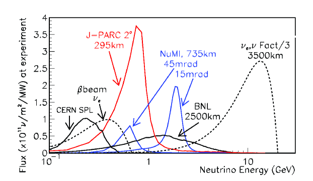
Figure 39: Neutrino fluxes for several of the proposed experiments. Taken from Ref. [306].

In general, the independent determination of the missing pieces of the puzzle at these experiments becomes challenging because in the relevant oscillation probabilities there appear three independent two-fold parameter degeneracies [308, 309, 310, 311]. In brief:

• ($\theta_{23}$, $\pi/2-\theta_{23}$) degeneracy [312, 308] which means that the same event rates are predicted for a value of $\theta_{23}$ mixing angle than for the value $\pi/2-\theta_{23}$. This is due to the fact that most sensitivity to the $\theta_{23}$ angle is achieved from precise measurement of $\nu_{\mu}$ disappearance and the dominant piece of the relevant probability Eq. (298), is invariant under the exchange $\theta_{23}\to\pi/2-\theta_{23}$.

• ($\delta_{\text{CP}}$, $\theta_{13}$) degeneracy [309]. This means that by simultaneously changing $(\delta_{\text{CP}}$ and $\theta_{13})$ it is possible to predict the same number of observed events. This is due to the fact that the appearance probability Eq. (297) takes the same values for different pairs of parameters ($\delta_{\text{CP}}$, $\theta_{13}$).

• The third degeneracy arises because it is possible to change simultaneously the sign of $\Delta m^{2}_{31}$ and the value of $\delta_{\text{CP}}$ without changing the predicted number of observed events. It arises from the fact that in Eq. (297) a change in $\mathop{\mathrm{sgn}}(\Delta m^{2}_{31})$ can be compensated by an offset in $\delta_{\text{CP}}$ [310, 311].

As a consequence if one only measures the total number of events in the different channels at a given facility (fixed $L$) one can find different sets of parameters which are able to fit the data.

The phenomenological efforts in this front concentrate on the study of how the combination of data from experiments performed at different baselines and/or with different beam types [313, 314, 315, 316] as well as the use of subdominant oscillation channels involving $\nu_{\tau}$’s [317] and the measurement of the energy spectrum of the events [318, 319, 320] can help in resolving these degeneracies.

Next we briefly describe the expectations at some of these proposed facilities.

7.3 First Generation of Superbeam and Reactor Experiments

There are two different type of experiments being built or proposed as a first step in the determination of the full leptonic mixing matrix. They make use of either a neutrino superbeam with an detector off axis or a reactor antineutrino beam with a near and far detector.

Neutrino superbeams are defined as conventional neutrino beams produced using megawatt-scale high-energy proton drivers. The conventional neutrino beam is produced using the very powerful primary proton beam which after hitting a target, creates a secondary beam composed mostly of charged pions and some kaons. They are then allowed to decay to produce a tertiary neutrino beam. The secondary beam are focused and allowed to decay in a long decay channel and it can be charge-sign selected to produce either a neutrino beam from positive meson decays or an antineutrino beam from negative meson decays.

The resulting neutrino beam consists mostly of muon neutrinos (or antineutrinos) from $\pi^{\pm}\to\mu+\nu_{\mu}$ decays, with a small “contamination” of electron neutrinos, electron antineutrinos, and muon antineutrinos from muon, kaon, and charmed meson decays. The fractions of $\nu_{e}$, $\bar{\nu}_{e}$ and $\bar{\nu}_{\mu}$ in the beam depend critically on the beamline design.

The contamination from other neutrino species is a handicap for the appearance experiments searching for $\nu_{\mu}\to\nu_{e}$ transition, which as we have seen above, is the dominant channels in the determination of $\theta_{13}$, the mass ordering and the CP phase. However, the signal to noise ratio can be improved if one could design a conventional superbeam which was nearly monochromatic. In order to made such a narrow band neutrino beam the off-axis [321] technique is being put forward. The basic point is that because the pion decay is a two-body decay, there is an angle with respect to the focused pion direction where the broad band of pion energies will produce a narrow band of neutrino energies. In the near future two narrow band beams are being foreseen: one for the T2K experiment in Japan [287] and another one using the Fermilab NuMI beamline [298, 299, 322].

T2K makes use of the new 0.8 MW hadron facility being constructed at JAERI, J-PARC with an initial proton energy of 40 GeV. In combination with that facility there will be a neutrino beam line which will be aimed at the Super-Kamiokande detector. This off axis beam will allow the T2K experiment to run at peak neutrino energies between 550 and 700 MeV.

At Fermilab the NuMI beamline, while providing on axis neutrinos for the MINOS experiment, is also producing off axis neutrinos. For example a detector place at about 20mrad from the NuMI beamline would see a very narrow neutrino beam peaked at 2 GeV. Using this idea the NO$\nu$a concept [298, 299] was proposed to used a fine grained calorimeter based on liquid scintillator as a detector. Also, a proposal to use a Liquid Argon Time Projection Chamber as a detector, FLARE [322], has been put forward,

In addition to the intrinsic background due to the beam contamination, the appearance experiments are also challenged by the background due to neutral current $\pi^{0}$ production in the detector which mimics the electron neutrino signal. The relevance of this background is different for different detection techniques and it seems better eliminated with a liquid argon type detector.

Recently, there has been a lot of activity to investigate the potential of new reactor neutrino experiments [300] based on the observation that the performance of previous experiments, such as CHOOZ [83], can be significantly improved if a near detector is used to control systematics and if the statistics is increased. The main advantage of these experiments is that they are free of degeneracies as they only measure the disappearance probability Eq. (299) which gives a direct determination of $\theta_{13}$.

A number of possible sites are discussed, including reactors in Brasil, China, France, Japan, Russia, Taiwan, and the US (see Ref [300, 301] for an extensive list). Of these projects the Double-Chooz experiment [323] has the opportunity to obtain results first. The experiment will employ two almost identical detectors of medium size. The far detector will be situated in the same cavern as CHOOZ but will be able detect  50000 electron antineutrinos in three years of operation with a systematic uncertainty of 0.6%. From the second generation reactor experiments, a more advance project is the experiment proposed to be located in Daya Bay [324], China. Its basic layout consists of three underground experimental halls, one far, two near where eight identical cylindrical detectors will be located (four of them at the far site). The goal of the Daya Bay experiment is to reach a sensitivity of 0.01 or better in $\sin^{2}2\theta_{13}$ at 90% CL.

As illustration of the expectations in these experiments we show in Fig. 40 the results from Ref. [325] on the expected precision in the determination of $\Delta m^{2}_{31}$, $\theta_{23}$ and their sensitivity to $\theta_{13}$. From these results we read that the largest improvement is expected in the determination of $|\Delta m^{2}_{32}|$ whose uncertainty can be reduced to about a 10% while only a mild improvement is expected in the determination of $\theta_{23}$ because these experiments are mainly sensitive only to $\sin^{2}2\theta_{23}$.

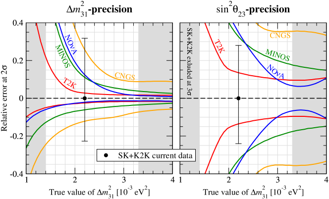
Figure 40: Expected sensitivity at near future oscillation experiments. Precision of $\Delta m^{2}_{31}$ (left), and $\sin^{2}\theta_{23}$ (center) as a function of the true value of $\Delta m^{2}_{31}$ ($\theta_{23}^{\text{true}}=\pi/4$), and sensitivity to $\sin^{2}2\theta_{13}$ (right) for $\Delta m^{2}_{31}=2\times 10^{-3}~{}\text{eV}^{2}$. See Ref. [325] for details.

The expected sensitivity to $\theta_{13}$ is given in the lower panel of Fig. 40. In this figure, from Ref. [325], systematics refers to the usual experimental and theoretical systematic errors such as errors in the overall signal and background normalization as well as in their energy dependence, uncertainties in the reconstruction efficiencies etc…. Correlation and degeneracy uncertainties refer to those which arise because, as discussed above, the relevant probabilities are dominantly sensitive to certain parameter combinations so the same event rates can be predicted with for different sets of parameters.

As seen in the figure the limit on $\theta_{13}$ from superbeam experiments is strongly affected by parameter correlations and degeneracies, whereas reactor experiments provide a “clean” measurement of $\theta_{13}$ whose precision is dominated by statistics and systematics (see Ref. [325] for details).

The results from Ref. [325] show also that a non zero value of $\theta_{13}$ close to their present bound would be established in any of these experiments. However none of them on their own can give any information on the CP-phase $\delta_{\text{CP}}$ and on the mass hierarchy because of the correlations. Some information on these parameters can only be obtained if $\theta_{13}$ is close to their present bound and the results from several of the experiments are combined.

7.4 Far Future LBL Experiments

In the longer term future one can think of proton driver upgrades of existing proton sources. For example if the proton sources at either Fermilab or J-PARC or both were upgraded to 2 or even 4 MW, the mass ordering could be determined in a larger region of parameter space. Furthermore a larger detector as well as running both in the neutrino and the antineutrino mode are considered a requirement to be able to detect CP violation.

At CERN a proposal to build a neutrino superbeam using the Super Proton Linac (SPL) which would provide a 2.2 GeV proton beam of 4 MW has been studied [326]. This would be a low energy conventional broad band $\nu_{\mu}$ beam aimed at a large water Cherenkov detector located in Frejus, 130 km away. In principle at this short distance matter effects are very small and they do not affect the precision at which the experiment could observe CP violation. On the other hand, for the same reason, the experiment cannot yield any information on the mass ordering.

Another proposal for the search for oscillation in a higher energy broad band beam is the Brookhaven proposal [327]. With this beam aimed at a large water Cherenkov detector located at a baseline of about 2500 km the experiment would be able to see matter effects at the high energy part of the neutrino spectrum as well CP violating effects at lower energies [319].

Ultimately the presence of backgrounds that fake $\nu_{e}$ CC interactions, together with a small $\nu_{e}$ component in the initial beam, make it difficult for experiments using conventional neutrino beams to probe very small oscillation amplitudes, below the $0.01-0.001$ range. This limitation motivates new types of neutrino facilities that provide $\nu_{e}$ beams, permitting the search for $\nu_{e}\to\nu_{\mu}$ oscillations, and if the beam energy is above the $\nu_{\tau}$ CC interaction threshold, the search for $\nu_{e}\to\nu_{\tau}$ oscillations. Neutrino Factory and Beta Beam facilities both provide $\nu_{e}$ (and $\bar{\nu}_{e}$) beams, but with somewhat different beam properties.

7.4.1 $\beta$ Beams

The idea of a Beta Beam facility was first proposed by P. Zucchelli in 2002 [305]. As the name suggests, it employs beams of beta-unstable nuclides. By accelerating these ions to high energy and storing them in a decay ring a very pure beam of electron neutrinos (or antineutrinos) can be produced. As the kinematics of the beta decay is well understood, the energy distribution of the neutrinos can be predicted to a very high accuracy. Furthermore, as the energy of the beta decay is low compared with that for muon decay, the resulting neutrino beam has a small divergence.

For low-$Z$ beta-unstable nuclides, typical decay times are measured in seconds. Thus, there is not high a premium on rapid acceleration and conventional (or even existing) accelerators could be used for acceleration in a Beta Beam facility. Two ion species, both having lifetimes on the order of 1 s, have been identified as optimal candidates: ${}^{6}\text{He}$ for producing antineutrinos and ${}^{18}\text{Ne}$ for neutrinos. Also the possibility of generating a monochromatic neutrino beam using recently discovery isotopes that decay fast through electron capture [328] has been studied. Recently the capabilities of a very long baseline Beta Beam experiment using radioactive ${}^{8}\text{B}$ and ${}^{8}\text{Li}$ as the source isotopes for the $\nu_{e}$ and $\bar{\nu}_{e}$ beta-beam has also been explored [329].

The original Beta Beam proposal [330] was to use the CERN SPS to accelerate the ions in combination with a large detector in the Frejus tunnel in France which would yield mean neutrino and antineutrino energies of 0.2 GeV and 0.3 GeV ($L=130$ km) respectively. However the expected signal rates are relatively modest. In addition, it has been pointed out [331] that the neutrino energies are comparable to the target nucleon kinetic energies due to Fermi motion, and therefore there is no useful spectral information in the low energy Beta Beam measurements. Hence, the useful information is restricted to the measured muon neutrino (and antineutrino) appearance rates. Hence higher energy scenarios are being considered [331, 332]. A medium energy beta beam experiment could be obtained using the Fermilab Tevatron for acceleration (yielding mean neutrino and antineutrino energies of 1.2 GeV and 1.9 GeV respectively), and a 1 megaton water Cherenkov detector in the Soudan mine ($L=730$ km). A high energy beta beam experiment would require the CERN LHC to accelerate the ions (mean neutrino and antineutrino energies of 5 GeV and 7.5 GeV respectively) and a very long baseline, $L=3000$ km.

The sensitivity at these Beta Beam scenarios is illustrated in Fig. 41 from Ref. [331]

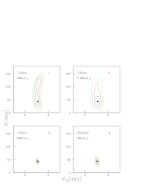
Figure 41: (Low-Energy (I), Medium-Energy (II), and High-Energy (III) Beta Beam sensitivities. The estimated $\,1\sigma,2\,\sigma$ and $3\,\sigma$ contours are shown for the setups described in the text. See Ref. [331].

The figure shows, for the three scenarios, the $1\sigma$, $2\sigma$, and $3\sigma$ contours in the ($\theta_{13},\,\delta_{\text{CP}}$) plane. Note that the expected sensitivity for the medium energy case with a “small” water Cherenkov detector is comparable to the low energy case with the megaton water Cherenkov detector. However, the medium energy sensitivity is dramatically improved with the much bigger detector. The further improvement obtained by going to LHC energies seems to be marginal. Given the likelihood that the LHC would not be available as a Beta Beam accelerator for a very long time, perhaps the most interesting scenario is the medium energy one.

Preliminary results on the capabilities of this intermediate energy beta beam [332] seems to indicate that the problem of discrete ambiguities due to degeneracies and their bias in the determination of $\theta_{13}$ and $\delta_{\text{CP}}$ can be solved down to somewhat smaller values of $\theta_{13}$ ($\sin^{2}2\theta_{13}\gtrsim\mathcal{O}(5\times 10^{-5})$) than with a Superbeam.

7.4.2 Neutrino Factories

For a Neutrino Factory, the production beam is a high intensity proton beam of moderate energy (beams of $2-50$ GeV have been considered by various groups) that impinges on a target, typically a high-$Z$ material. The collisions between the proton beam and the target nuclei produce a secondary pion beam that quickly decays into a longer-lived muon beam. The remainder of the Neutrino Factory is used to condition the muon beam, accelerate it rapidly to the desired final energy of a few tens of GeV, and store it in a decay ring having a long straight section oriented such that decay neutrinos produced there will hit a detector located thousands of kilometers from the source.

At a Neutrino Factory in which, for example, positive muons are stored, the initial beam consists of 50% $\nu_{e}$ and 50% $\bar{\nu}_{\mu}$. The energy spectrum of both type of neutrinos at the detector site is different for the two flavors and it is given in terms of the very well known $\mu$ decay distribution. Therefore it can be predicted with very high precision.

In the absence of oscillations, the $\nu_{e}$ CC interactions produce electrons and the $\bar{\nu}_{\mu}$ CC interactions produce positive muons. Note that the charge of the final state lepton tags the flavor of the initial neutrino or antineutrino. In the presence of $\nu_{e}\to\nu_{\mu}$ oscillations, the $\nu_{\mu}$ CC interactions produce negative muons (i.e., wrong-sign muons). This is a very clean experimental signature since, with a segmented magnetized iron-scintillator sampling calorimeter for example, it is straightforward to suppress backgrounds to 1 part in $10^{4}$ of the total CC interaction rate, or better. This means that at a Neutrino Factory backgrounds to the $\nu_{e}\to\nu_{\mu}$ oscillation signal are extremely small. The full statistical sensitivity can therefore be exploited down to values of $\sin^{2}2\theta_{13}$ approaching $10^{-4}$ before backgrounds must be subtracted and further advances in sensitivity scale like $\sqrt{N}$ rather than $N$. This enables Neutrino Factories to go beyond the sensitivities achievable by conventional neutrino Superbeams and $\beta$ beams, by about two orders of magnitude.

In practice, to measure $\theta_{13}$, determine the mass hierarchy, and search for CP violation, the analysis of the wrong-sign muon rates must be performed allowing all of the oscillation parameters to simultaneously vary within their uncertainties which leads us again to the possible problem of parameter degeneracies. As an illustration we show in Fig. 42 (from Ref. [333]), as a function of $\theta_{13}$, $\theta_{23}$, $\delta_{\text{CP}}$ and the assumed mass ordering, the predicted number of wrong-sign muon events when negative muons are stored in the Neutrino Factory, versus the corresponding rate when positive muons are stored. Given the large statistics expected the statistical errors would be barely visible if plotted. Thus for the parameter region illustrated by the figure, determining the mass hierarchy (which diagonal line is the measured point closest to) will be straightforward. But determining the exact values for the mixing angles and $\delta_{\text{CP}}$ is more complicated because of the degeneracies.

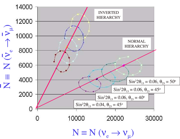
Figure 42: The predicted number of wrong-sign muon events when negative muons are stored in the Neutrino Factory, versus the corresponding rate when positive muons are stored, shown as a function of $\theta_{13}$, $\theta_{23}$, $\delta_{\text{CP}}$ and the assumed mass hierarchy, as labeled. The calculation corresponds to a 16 GeV Neutrino Factory with a baseline of 2000 km, and 10 years of data taking with a 100 kton detector and $2\times 10^{20}\,\mu^{+}$ and $2\times 10^{20}\,\mu^{-}$ decays in the beam-forming straight section per year. The ellipses show how the predicted rates vary as the CP phase $\delta_{\text{CP}}$ varies. See Ref. [333] for details.

To eliminate the false solutions, event samples other than $\nu_{e}\to\nu_{\mu}$ transitions tagged by wrong-sign muons will be important. For example $\bar{\nu}_{\mu}\to\bar{\nu}_{e}$ oscillations produce wrong-sign electrons, $\bar{\nu}_{\mu}\to\bar{\nu}_{\tau}$ oscillations produce events tagged by a $\tau^{+},$ and $\nu_{e}\to\nu_{\tau}$ oscillations produce events tagged by a $\tau^{-}$. Hence, there is a variety of information that can be used to measure or constrain neutrino oscillations at a Neutrino Factory, namely the rates and energy distributions of all these different event types. If these measurements are made when there are alternately positive and negative muons decaying in the storage ring, there are a total of 12 spectra that can be used to extract information about the oscillations.

The overall conclusion of the different simulations [318, 317, 334, 320, 335, 336] (see also Ref. [304, 326, 337] for detailed reviews) is that at a Neutrino Factory ${\sin^{2}2\theta_{13}}$ can be measured, the neutrino mass hierarchy determined, and a search for CP violation in the lepton sector made for all values of $\sin^{2}2\theta_{13}$ down to O$(10^{-4}$), or even a little less.

7.5 Future Atmospheric Neutrino Experiments

As seen in previous sections, large next generation underground water Cherenkov detectors are proposed in US, in Japan and in Europe [285, 286, 287, 288]. These large megaton class detectors are proposed as multi-purpose detectors that probe physics beyond the sensitivities of the highly successful Super-Kamiokande detector utilizing a well- tested technology. The physics goals of these detectors include: nucleon decay searches, observation of neutrinos from supernova explosions, observation of supernova relic neutrinos, and precision measurements of neutrino oscillation parameters using atmospheric, solar and accelerator produced neutrinos.

There are also plans to build a 30-50 kton magnetized tracking iron calorimeter detector in India within the India-based Neutrino Observatory (INO) project [338] with the primary goal of studying the oscillations of atmospheric $\nu_{\mu}$ and $\bar{\nu}_{\mu}$. This detector is planned to have efficient muon charge identification, high muon energy resolution ($\sim 5\%$) and muon energy threshold of about 2 GeV. Although there are no details studies of the capabilities of such detector, its sensitivity should be comparable to that evaluated for an earlier proposal for a similar detector, MONOLITH [339]).

It is also worth noticing that presently running experiments whose main goal is not the study of atmospheric neutrinos will also have some reasonable samples of atmospheric events. For example SNO despite its relatively small size, thanks to its depth and flat overburden, can measure the atmospheric neutrino flux using through-going muons even above the detector horizon (up to $\cos\eta=0.4$) without any contamination from cosmic ray muons. These data above the horizon can tell us the unoscillated flux of neutrinos and therefore reduce the uncertainty of atmospheric neutrino flux models. In addition, the charged current interactions of antineutrinos within SNO should produce additional neutrons compared to neutrinos, and it may be possible to make a crude measurement of the relative rates of neutrinos versus antineutrinos. Also MINOS [90] is an iron magnetized calorimeter and thus, has muon charge identification capabilities for multi-GeV atmospheric muon events. In 2007 they reported a total of 140 neutrino-induced muon events and an observed charge ratio in agreement with expectations [340]. After 5 years of data-taking MINOS is expected to collect about 440 atmospheric $\nu_{\mu}$ and about 260 atmospheric $\bar{\nu}_{\mu}$ multi-GeV contained events.

The wide dynamic range of neutrino energies and baselines in the atmospheric sector mean that these future atmospheric neutrino experiments will provide their own tests of the oscillation model with the corresponding precision measurement of the dominant oscillation parameters $\Delta m^{2}_{32}$ and $\theta_{23}$. As an illustration of their precision we show in Fig. 43 the oscillation pattern which could be observed by the UNO detector using atmospheric neutrino events.

Figure 43: Simulated oscillation pattern observable by UNO [285, 286].

Furthermore, as discussed in Sec. 3.3 atmospheric neutrinos are in principle sensitive to $\theta_{13}$ and the neutrino mass hierarchy due to Earth matter effects in the $e$-like events. In addition effects from the solar parameters $\theta_{12}$ and $\Delta m_{21}^{2}$ on $e$-like events in the sub-GeV energy range provide sensitivity to the octant of $\theta_{23}$ and principle even on $\delta_{\text{CP}}$. In general, the precision expected for most of these effects from atmospheric data on its own is smaller than the one achievable at long baseline experiments, in particular in the determination of $\theta_{13}$, $\delta_{\text{CP}}$, $|\Delta m_{31}^{2}|$, or $\sin^{2}2\theta_{23}$. One reason is that atmospheric neutrino experiments are limited by systematical uncertainties, such as the theoretical uncertainties on the atmospheric neutrino fluxes and the interaction cross sections. A recent analysis of the capabilities of a future large water Cherenkov detector to determine these subdominant effects can be found in Ref. [341].

However, due to these effects atmospheric neutrino data can have an important role in breaking the parameter degeneracies (see Sec. 7.2) which appear in the analysis of long baseline experiments [342, 343], in particular the degeneracies associated to the octant of $\theta_{23}$ and the sign($\Delta m^{2}_{31}$). As an illustration of their potential we show in Fig. 44 the allowed regions from the analysis of the phase II of the T2K experiment assuming a 4 MW superbeam produced at the J-PARC accelerator, and the 1 Mt Hyper-Kamiokande [288] detector serving as the far detector for the LBL experiment as well as providing the high statistics atmospheric neutrino data. The figure shows the allowed regions in the $(\sin^{2}2\theta_{13},\,\delta_{\text{CP}})$ plane for an example-point with the true values $\sin^{2}2\theta_{13}=0.03$, $\delta_{\text{CP}}=-0.85\pi$, and non-maximal values of $\theta_{23}^{\text{true}}$. Apart from the true solution, three degenerate regions are present, corresponding to the wrong octant of $\theta_{23}$, the wrong sign of $\Delta m_{31}^{2}$, and the wrong octant as well as the wrong hierarchy.

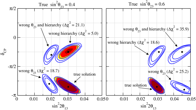
Figure 44: Allowed regions in the $(\sin^{2}2\theta_{13},\,\delta_{\text{CP}})$ plane at $2\sigma$, 99%, and $3\sigma$ CL (2 d.o.f.) of the true and all degenerate solutions for $\sin^{2}2\theta_{13}^{\text{true}}=0.03$, $\delta^{\text{true}}=-0.85\pi$, and $\sin^{2}\theta_{23}^{\text{true}}=0.4$ (left) and $\sin^{2}\theta_{23}^{\text{true}}=0.6$ (right). The solid curves correspond to LBL data only, and the shaded regions correspond to LBL+ATM data. The true best fit point is marked with a star, the best fit points of the degenerate solutions are marked with dots, and the corresponding $\Delta\chi^{2}$-values of LBL+ATM data are given in the figure. The true mass ordering is the normal hierarchy.

This four-fold degeneracy can be lifted to large extent if LBL data is combined with data from atmospheric neutrinos. As seen in the figure the degenerate solutions corresponding to the wrong octant of $\theta_{23}$ are highly disfavored by the inclusion of ATM data. Furthermore, also the solution with the wrong mass ordering gets disfavored in the combined analysis, although in this case the ability to resolve this degeneracy is more subtle. This is due to the fact that in a water-Cherenkov detector the distinction between neutrino and antineutrino events is not possible (on an event-by-event basis). This makes more difficult the determination of the mass ordering which is only feasible due to the difference of fluxes and cross sections for neutrinos and antineutrinos. The ability to resolve the mass ordering is expected to be much better if the atmospheric neutrino detector is a magnetized calorimeter which has the capability of discriminating the charge of the neutrino-induced muon [128, 339].

8 Direct Determination of $m_{\nu}$

Oscillation experiments have provided us with important information on the differences between the neutrino masses-squared, $\Delta m^{2}_{ij}$, and on the leptonic mixing angles, $U_{ij}$. But they are insensitive to the absolute mass scale for the neutrinos, $m_{i}$.

Of course, the results of an oscillation experiment do provide a lower bound on the heavier mass in $\Delta m^{2}_{ij}$, $|m_{i}|\geq\sqrt{\Delta m^{2}_{ij}}$ for $\Delta m^{2}_{ij}>0$. But there is no upper bound on this mass. In particular, the corresponding neutrinos could be approximately degenerate at a mass scale that is much higher than $\sqrt{\Delta m^{2}_{ij}}$. Moreover, there is neither upper nor lower bound on the lighter mass $m_{j}$. In this section we briefly summarize the most sensitive probes of the absolute mass scale for the neutrinos.

8.1 Kinematic Constraints from Weak Decays

It was Fermi who first proposed a kinematic search for the neutrino mass from the hard part of the beta spectra in ${}^{3}\text{H}$ beta decay ${}^{3}\text{H}\to^{3}\text{He}+e^{-}+\bar{\nu}_{e}$. In the absence of leptonic mixing this search provides a measurement of the electron neutrino mass.

${}^{3}\text{H}$ beta decay is a superallowed transition, which means that the nuclear matrix elements do not generate any energy dependence, so that the electron spectrum is given by the phase space alone

$$\frac{dN}{dE}=C\,p\,E\,(Q-T)\sqrt{(Q-T)^{2}-m_{\nu_{e}}^{2}}F(E)\equiv R(E)\sqrt{(E_{0}-E)^{2}-m_{\nu_{e}}^{2}}\,.$$ (303)

where $E=T+m_{e}$ is the total electron energy, $p$ its momentum, $Q\equiv E_{0}-m_{e}$ is the maximum kinetic energy of the electron and $F(E)$ is the Fermi function which incorporates final state Coulomb interactions. In the second equality we have included in a $R(E)$ all the $m_{\nu}$-independent factors.

Plotted in terms of the Curie function $K(T)\equiv\sqrt{\frac{dN}{dE}\,\frac{1}{pEF(E)}}$ a non-vanishing neutrino mass $m_{\nu}$ provokes a distortion from the straight-line T-dependence at the end point: for $m_{\nu}=0\Rightarrow T_{\text{max}}=Q$ whereas for $m_{\nu_{e}}\neq 0\Rightarrow T_{\text{max}}=Q-m_{\nu_{e}}$. ${}^{3}\text{H}$ beta decay has a a very small energy release $Q=18.6$ KeV which makes it particularly sensitive to this kinematic effect.

At present the most precise determination from the Mainz [344] and Troitsk [345] experiments give no indication in favor of $m_{\nu_{e}}\neq 0$ and one sets an upper limit

$$m_{\nu_{e}}<2.2~{}\text{eV}$$ (304)

at 95% confidence level (CL). For the other flavors the present limits are [23]

$$m_{\nu_{\mu}} <190~{}\text{keV (90\% CL)} \pi^{-}\to\mu^{-}+\bar{\nu}_{\mu}\,,$$ from (305)

$$m_{\nu_{\tau}} <18.2~{}\text{MeV (95\% CL)} \tau^{-}\to n\pi+\nu_{\tau}\,.$$ from (306)

In the presence of mixing these limits have to be modified and in general they involve more than one flavor parameter. For neutrinos with small mass differences the distortion of the beta spectrum is given by the weighted sum of the individual spectra [346]:

$$\frac{dN}{dE}=R(E)\sum_{i}|U_{ei}|^{2}\sqrt{(E_{0}-E)^{2}-m_{i}^{2}}\,\Theta(E_{0}-E-m_{i})\,.$$ (307)

The step function, $\Theta(E_{0}-E-m_{i})$, reflects the fact that a given neutrino can only be produced if the available energy is larger than its mass. According to Eq. (307), there are two important effects, sensitive to the neutrino masses and mixings, on the electron energy spectrum: (i) Kinks at the electron energies $E_{e}^{(i)}=E\sim E_{0}-m_{i}$ with sizes that are determined by $|U_{ei}|^{2}$; (ii) A shift of the end point to $E_{\text{ep}}=E_{0}-m_{1}$, where $m_{1}$ is the lightest neutrino mass. The situation is slightly more involved when the finite energy resolution of the experiment is considered [347, 348].

In general for most realistic situations the distortion of the spectrum can be effectively described by a single parameter, $m_{\beta}$ if for all neutrino states $E_{0}-E=Q_{0}-T\gg m_{i}$. In this case one can expand Eq. (307) as:

$$\frac{dN}{dE} \simeq R(E)\sum_{i}|U_{ei}|^{2}(E_{0}-E)\left(1-\frac{m_{i}^{2}}{2(E_{0}-E)}\right)$$ (308)

$$=R(E)\,\sum_{i}|U_{ei}|^{2}\,(E_{0}-E)\left(1-\frac{1}{2(E_{0}-E)}\frac{\sum_{i}|U_{ei}|^{2}m^{2}_{i}}{\sum_{i}|U_{ei}|^{2}}\right)$$

$$\simeq R(E)\sum_{i}|U_{ei}|^{2}\sqrt{(E_{0}-E)^{2}-m_{\beta}^{2}}\,,$$

with

$$m^{2}_{\beta}=\frac{\sum_{i}m^{2}_{i}|U_{ei}|^{2}}{\sum_{i}|U_{ei}|^{2}}=\sum_{i}m^{2}_{i}|U_{ei}|^{2}\,,$$ (309)

where the second equality holds if unitarity is assumed. So the distortion of the end point of the spectrum is described by a single parameter which is bounded to be

$$m_{\beta}=\sqrt{\sum_{i}m^{2}_{i}|U_{ei}|^{2}}<2.2~{}\text{eV}\,.$$ (310)

A new experimental project, KATRIN [349], is under construction with an estimated sensitivity limit: $m_{\beta}\sim 0.3$ eV.

8.2 Neutrinoless Double Beta Decay

Direct information on neutrino masses can also be obtained from neutrinoless double beta decay ($0\nu\beta\beta$) searches:

$$(A,Z)\to(A,Z+2)+e^{-}+e^{-}.$$ (311)

Schematically in the presence of neutrino masses and mixing the process in Eq. (311) can be induced by the diagram shown in Fig. 45. The amplitude of this process is proportional to the product of the two leptonic currents

$${M}_{\alpha\beta}\propto\left[\bar{e}\gamma_{\alpha}(1-\gamma_{5})\nu_{e}\right]\,\left[\bar{e}\gamma_{\beta}(1-\gamma_{5})\nu_{e}\right]\,.$$ (312)

which can only lead to a neutrino propagator from the contraction $\langle 0\,|\,\nu_{e}(x)\nu_{e}(y)^{T}\,|\,0\rangle$. If the neutrino is a Dirac particle $\nu_{e}$ field annihilates a neutrino states and creates an antineutrino state which are different. Therefore the contraction $\langle 0\,|\,\nu_{e}(x)\nu_{e}(y)^{T}\,|\,0\rangle=0$ and $M_{\alpha\beta}=0$. On the contrary, if $\nu_{e}$ is a Majorana particle, neutrino and antineutrino are the same state and $\langle 0\,|\,\nu_{e}(x)\nu_{e}(y)^{T}\,|\,0\rangle\neq 0$.

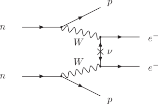
Figure 45: Feynman diagram for neutrinoless double-beta decay.

Thus in order to induce the $0\nu\beta\beta$ decay, $\nu_{e}$ must be a Majorana particle. This is also obvious as the process (311) violates L by two units. The opposite also holds, if $0\nu\beta\beta$ decay is observed, neutrinos must be massive Majorana particles [350].

However, Majorana neutrino masses are not the only mechanism which can induce neutrinoless double beta decay. In general, in models beyond the standard model there may be other sources of total lepton number violation which can induce $0\nu\beta\beta$ decay. Consequently the observation or limitation of the neutrinoless double beta decay reaction rate can only be related to a bound on the neutrino mass and mixing under some assumption about the source of total lepton number violation in the model.

For the case in which the only effective lepton number violation at low energies is induced by the Majorana mass term for the neutrinos, the rate of $0\nu\beta\beta$ decay is proportional to the effective Majorana mass of $\nu_{e}$,

$$m_{ee}=\left|\sum_{i}m_{i}U_{ei}^{2}\right|$$ (313)

which, in addition to the masses and mixing parameters that affect the tritium beta decay spectrum, depends also on the leptonic CP violating phases.

Experimentally, what it is measured is the half-life of the decay. In $0\nu\beta\beta$ decay, the experimental signal is two electrons in the final state, whose energies add up to the Q-value of the nuclear transition while for the double beta decay with neutrinos ($2\nu\beta\beta$) (which constitute an intrinsic background) the energy spectrum of both electrons will be continuous as part of the Q is carried by the outgoing neutrinos. Also the decay rates for $0\nu\beta\beta$ and $2\nu\beta\beta$ have very different dependence on the available Q being the dependence much weaker for $0\nu\beta\beta$. For this reason, the sensitivity is better for isotopes with a high Q-value.

In the case that the only source of lepton number violation at low energies is induced by the Majorana neutrino mass, the decay half-life is given by:

$$(T^{0\nu}_{1/2})^{-1}=G^{0\nu}\left|M^{0\nu}\right|^{2}\left(\frac{m_{ee}}{m_{e}}\right)^{2}$$ (314)

where $G^{0\nu}$ is the phase space integral and $|M^{0\nu}\mid$ is the nuclear matrix element of the transition.

The strongest bound from $0\nu\beta\beta$ decay was imposed by the Heidelberg-Moscow group [351] which used 11 kg of enriched Ge. After 53.9 kg yr of data taking they found no signal which allowed them to set a bound on the half-life of $T^{0\nu}_{1/2}>1.9\times 10^{25}$ yr (90% CL). This implies (for a given prediction of the nuclear matrix element):

$$m_{ee}<0.26~{}(0.34)~{}\text{eV}\quad\text{at 68\% (90\%) CL.}$$ (315)

Taking into account the possible uncertainties in the prediction of the nuclear matrix elements, the bound may be weaken by a factor of about 3 [352].

Despite the result of the Heidelberg-Moscow experiment is that no positive signal was observed, a subgroup of the collaboration found a small peak at some value of $Q$ [353, 354] which, if real, would imply a non vanishing range for the effective Majorana mass between $0.2$–$0.6$ eV (the range might be widened by nuclear matrix uncertainties). However, the statistical analysis used, as well as the assumed background subtraction in order to establish this evidence at the claimed CL has been subject of severe criticisms [355, 356, 357, 358] which renders the claimed signal as controversial.

Currently only two large scale experiments are running. CUORICINO at the Gran Sasso Underground Laboratory in Italy which uses uses bolometers running at very low temperature and searches for ${}^{120}\text{Te}$ decay with a Q-value of 2530 keV. The obtained half-life limit [359] $T^{0\nu}_{1/2}(^{120}\text{Te})>2.2\times 10^{24}$ yr (90% CL) implies and upper bound on the effective Majorana neutrino mass $m_{ee}<0.2$–$1.1$ eV. The second experiment, NEMO-3 [360] in the Frejus Underground Laboratory, is built in form of time projection chambers where the double beta emitter is either the filling gas of the chamber or is included in thin foils. It has obtained a half-life bound for ${}^{100}\text{Mo}$ $T^{0\nu}_{1/2}(^{100}\text{Mo})>5.6\times 10^{23}$ yr (90% CL) which result in an upper effective Majorana mass bound $m_{ee}<0.6$–$2$ eV.

A series of new experiments is planned with sensitivity of up to $m_{ee}\sim 0.01$ eV. For a review of the proposed experimental techniques see Ref. [361, 362].

8.3 Cosmological Bounds

Neutrinos, like any other particles, contribute to the total energy density of the Universe. Furthermore light neutrinos are relativistic through most of the evolution of the Universe. As a consequence they can play a relevant role in large scale structure formation and leave clear signatures in several cosmological observables. For an excellent recent review on the cosmological effects of neutrino masses we refer the reader to the report of J. Legourges ad S. Pastor [13].

The main effect of neutrinos in cosmology is to suppress the growth of fluctuations on scales below the horizon when they become non relativistic. As a consequence a massive neutrino of a fraction of eV would produce a significant suppression in the clustering on small cosmological scales. Because of this effect it is possible to infer constraints, although indirect, on the neutrino masses by comparing the most recent cosmological data with the theoretical predictions.

The relevant quantity in these studies is the total neutrino energy density in our Universe, $\Omega_{\nu}h^{2}$ (where $h$ is the Hubble constant normalized to $H_{0}=100~{}\text{km}~{}\text{s}^{-1}~{}\text{Mpc}^{-1}$). At present $\Omega_{\nu}h^{2}$ is related to the total mass in the form of neutrinos

$$\Omega_{\nu}h^{2}=\sum_{i}m_{i}/(94\text{eV})\,.$$ (316)

Therefore cosmological data mostly gives information on the sum of the neutrino masses $M_{\nu}=\sum_{i}m_{\nu_{i}}$ and has very little to say on their mixing structure.

The recent precise astrophysical and cosmological observations have started to provide us with indirect upper limits on absolute neutrino masses which are competitive with those from laboratory experiments. The most relevant data come from the Large Scale Structures (LSS) as obtained from large redshift surveys of galaxies by the 2 degree Field survey [363] and the Sloan Digital Sky Survey [364] and from Cosmic Microwave Background (CMB) anisotropies which at present are most precisely determined by the WMAP experiment [365]. Additional information can also be extracted from the so-called Lyman-$\alpha$ forest [366, 367]. This corresponds to the Lyman-$\alpha$ absorption of photons traveling from distant quasars ($z\sim 2-3$) by the neutral hydrogen in the intergalactic medium.

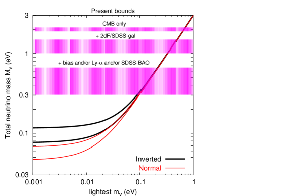
Figure 46: Current upper bounds (95% CL) from cosmological data on the sum of neutrino masses, compared to the values in agreement at a $3\sigma$ level with neutrino oscillation data. From Ref. [13]

As discussed in detail in Ref. [13] a single cosmological bound on neutrino masses does not exist. The bound depends on the data included in analysis as well as on details on the biases assumed and on the statistical treatment. For illustration we show in Fig. 46 the graphical summary given in Ref. [13]. In this figure the cosmological bounds obtained by different groups using a given set of data correspond to the horizontal bands. The thickness of these bands roughly describe the spread of values obtained from similar cosmological data: $2-3$ eV for CMB only, $0.9-1.7$ eV for CMB and 2dF/SDSS-gal or $0.3-0.9$ eV with the inclusion of a measurement of the bias and/or Lyman-$\alpha$ forest data and/or the SDSS measurement of the baryon oscillation peak. One can see from Fig. 46 that current cosmological data is only sensitive degenerate neutrino spectra with three neutrino states of the same mass, $M_{\nu}/3$. Using only the combined results of CMB and galaxy clustering data from 2dF and/or SDSS a conservative upper bound of $\sim$ 1 eV can be imposed. The addition of more data leads to an improvement of the bounds, which reach the lowest values when data from Lyman-$\alpha$ and/or the SDSS measurement of the baryon oscillation peak are included or the bias is fixed. Also, there are analysis in the literature for which the cosmological bounds are stronger than the 0.3 eV lowest value of the ranges quoted in the figure, such as in Ref. [368]. They make use of the data of LSS derived from the Lyman-$\alpha$ forest data and there is no consensus in the literature whether these can be used in the presence of massive neutrinos.

9 Extended Models for LSND

For years the most troublesome piece of experimental evidence in neutrino physics has been the result of the LSND experiment, which observed a small appearance of electron anti-neutrinos in a muon anti-neutrino beam at a value of $L/E$. The main reason for this is that the mass-squared differences required to explain the solar+KamLAND, atmospheric+LBL and LSND experimental results in terms of neutrino oscillations differ from one another by various orders of magnitude. Consequently, there is no consistent way to explain all these three signals invoking only oscillations among the three known neutrinos. The argument for this statement is very simple. With three neutrinos, there are only two independent mass-squared differences, since by definition:

$$\Delta m^{2}_{31}=\Delta m^{2}_{21}+\Delta m^{2}_{32}\,.$$ (317)

This relation cannot be satisfied by three $\Delta m^{2}_{ij}$ that are of different orders of magnitude. Therefore, in order to explain the LSND anomaly one had to invoke an extension of the three-neutrino mixing scenario, introducing either a mechanism to generate a third mass-square difference or a new form of flavor transition beyond oscillations.

After publication of the MiniBooNE result [110], which excluded the LSND signal at 98% CL in the context of two-neutrino $\nu_{\mu}\to\nu_{e}$ oscillations, some of these models have lost their main motivation, whereas other can be seen as ways to accommodate both results. In either case they all represent viable extensions of the minimal three-neutrino scenario, and in this section we summarize their present phenomenological status.

9.1 Four-Neutrino Mixing

One of the simplest extensions that one can think of to generate a third $\Delta m^{2}$ is to add a fourth neutrino to the SM. As discussed in Sec. 1.1, the measurement of the decay width of the $Z^{0}$ boson into neutrinos makes the existence of three, and only three, light (that is, $m_{\nu}\lesssim m_{Z}/2$) active neutrinos an experimental fact. Therefore, the fourth neutrino must not couple to the standard electroweak current, that is, it must be sterile.

One of the most important issues in the context of four-neutrino scenarios is the four-neutrino mass spectrum. In this section we review the status of four neutrino models in which the third mass difference is much larger than the ones required to explain the solar+KamLAND and the atmospheric+LBL results. The original motivation for these models was that the third mass difference was the one required to explain the LSND result. However, these scenarios cannot explain both a positive LSND result and the negative result of the search at MiniBooNE, so they are no longer a viable solution of the LSND puzzle. On the other hand, the existence of sterile neutrinos is an interesting subject by itself, irrespective of LSND, and four-neutrino models are the simplest extension of the Standard Model to include them. Therefore, in the following we will study the constraints on these models from the existing data.

There are six possible four-neutrino schemes, shown in Fig. 47, that can accommodate the results from solar and atmospheric neutrino experiments and contain a third much larger $\Delta m^{2}$. They can be divided in two classes: (3+1) and (2+2). In the (3+1) schemes, there is a group of three close-by neutrino masses that is separated from the fourth one by the larger gap. In (2+2) schemes, there are two pairs of close masses separated by the large gap. The main difference between these two classes is that in (2+2) models the extra sterile state cannot be simultaneously decoupled from both solar and atmospheric oscillations, whereas in (3+1) models the mixing between the sterile neutrino and the three active ones can be reduced at will. In other words, in (3+1) schemes it is possible to recover the usual three-neutrino scenario as a limiting case, whereas (2+2) schemes have unique phenomenological implications.

For what concerns the mixing parameters, we emphasize that the mixing matrix describing CC interactions in these schemes is a $3\times 4$ matrix. The reason is that there are three charged lepton mass eigenstates ($e,\,\mu,\,\tau$) and four neutrino mass eigenstates ($\nu_{1},\,\nu_{2},\,\nu_{3},\,\nu_{4}$). As discussed in Sec. 1.3, if we choose an interaction basis where the charged leptons are the mass eigenstates, then the CC mixing matrix $U$ is a sub-matrix of the $4\times 4$ unitary matrix $V^{\nu}$ that rotates the neutrinos from the interaction basis to the mass basis, where the line corresponding to $\nu_{s}$ is removed.

Figure 47: The six types of 4-neutrino mass spectra. The different distances between the masses on the vertical axes represent the different scales of mass-squared differences required to explain solar, atmospheric and LSND data with neutrino oscillations.

9.1.1 Status of (3+1) schemes

Well before the MiniBooNE experiment, it has been largely discussed in the literature that the (3+1)-spectra are strongly disfavored by the data from other SBL laboratory experiments [369, 370, 371, 372, 373, 374, 375, 376, 377, 378, 379] as explanations of the LSND result. This statement is based on a joint analysis of SBL experiments, which once combined with solar and atmospheric neutrino data severely constrain the simultaneous mixing of the sterile state with both $\nu_{e}$ and $\nu_{\mu}$. We summarize here these arguments and the present phenomenological status.

The probability $P_{\nu_{\mu}\to\nu_{e}}$ that is driven by the large $\Delta m^{2}_{41}$ (and which is relevant for LSND as well as KARMEN and NOMAD) is given by

$$P_{\nu_{\mu}\to\nu_{e}}=P_{\bar{\nu}_{\mu}\to\bar{\nu}_{e}}=4\,|U_{e4}U_{\mu 4}|^{2}\,\sin^{2}\frac{\Delta m^{2}_{41}L}{4E}\,,$$ (318)

where $L$ is the distance between source and detector. Here solar and atmospheric splittings have been neglected since they are too small to give any observable effect at the relevant $L/E$’s. In this approximation $\Delta m^{2}_{41}=\Delta m^{2}_{42}=\Delta m^{2}_{43}$ for schemes (3+1)A, and $\Delta m^{2}_{41}=\Delta m^{2}_{31}=\Delta m^{2}_{21}$ for schemes (3+1)B.

The LSND experiment gave an allowed region in the $(\Delta m^{2}_{41},\,|U_{e4}U_{\mu 4}|^{2})$ plane which can be directly obtained from the two-neutrino oscillation region shown in Fig. 7 with the identifications $\Delta m^{2}\to\Delta m^{2}_{41}$ and $\sin^{2}2\theta\to 4|U_{e4}U_{\mu 4}|^{2}$. In the same way, the KARMEN and MiniBooNE experiments gave an excluded region in the same plane which can be immediately derived from Fig. 7. As can be seen, practically all the LSND region is now excluded.

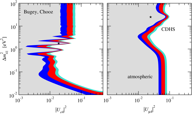
Figure 48: Bounds on $|U_{e4}|^{2}$ (left panel) and on $|U_{\mu 4}|^{2}$ (right panel) as a function of $\Delta m^{2}_{41}$. Different contours correspond to the two-dimensional allowed regions at 90%, 95%, 99% and $3\sigma$ CL. The best fit point is marked with a star.

Further constraints on $|U_{e4}U_{\mu 4}|^{2}$ can be obtained by combining the bounds on $|U_{e4}|$ and $|U_{\mu 4}|$ from reactor and accelerator experiments in combination with the information from solar and atmospheric neutrinos. The strongest constraints in the relevant $\Delta m^{2}_{41}$ region are given by the Bugey and CDHS experiments. Using their limits on the survival probabilities one finds

$$\begin{split}4|U_{e4}|^{2}\left(1-|U_{e4}|^{2}\right)&<D_{e}^{\text{Bugey}}(\Delta m^{2}_{41})\,,\\ D_{e}^{\text{Bugey}}&<0.001-0.1\quad\text{for}\quad 0.1\lesssim\Delta m^{2}_{41}/\text{eV}^{2}\lesssim 10\,,\end{split}$$ (319)

$$\begin{split}4|U_{\mu 4}|^{2}\left(1-|U_{\mu 4}|^{2}\right)&<D_{\mu}^{\text{CDHS}}(\Delta m^{2}_{41})\,,\\ D_{\mu}^{\text{CDHS}}&<0.05-0.1\quad\text{for}\quad\Delta m^{2}_{41}\gtrsim 0.5~{}\text{eV}^{2}\,,\end{split}$$ (320)

while for lower $\Delta m^{2}_{41}$ the CDHS bound weakens considerably. These bounds are plotted in Fig. 48 as a function of $\Delta m^{2}_{41}$. In principle, the inequalities in Eq. (319) and Eq. (320) can be satisfied with either small mixing parameters $|U_{\alpha 4}|^{2}\lesssim D_{\alpha}/4$, or close to maximal mixing, $|U_{\alpha 4}|^{2}\gtrsim 1-D_{\alpha}/4$. This is the generalization to these schemes of the symmetry $\theta\leftrightarrow\frac{\pi}{2}-\theta$ of two-neutrino vacuum oscillations (see Sec. 1.4). Solar and atmospheric data are invoked in order to resolve this ambiguity. Since in any of the allowed regions for solar oscillations $P^{\odot}_{ee}\lesssim 0.5$, only the small values of $|U_{e4}|$ are possible. For atmospheric neutrinos one can use the fact that oscillations with the large $\Delta m^{2}_{41}$ would wash-out the up-down asymmetry and this wash-out grows with the projection of the $\nu_{\mu}$ over states separated by the large $\Delta m^{2}_{41}$, which is controlled by the mixing parameter $|U_{\mu 4}|$. Consequently only the small values of $|U_{\mu 4}|$ are allowed. Thus naively one obtains the bound

$$4\,|U_{e4}U_{\mu 4}|^{2}<0.25\,D_{e}^{\text{Bugey}}(\Delta m^{2}_{41})\,D_{\mu}^{\text{CDHS}}(\Delta m^{2}_{41}).$$ (321)

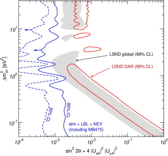
Figure 49: Upper bounds on $\sin^{2}2\theta=4|U_{e4}U_{\mu 4}|^{2}$ from the analysis of atmospheric+LBL+NEV data, in the context of (3+1)-schemes. Also shown are the regions allowed at 99% CL from the global LSND data and the decay-at-rest (DAR) LSND data. Adapted from Ref. [380].

A detailed and statistically meaningful evaluation of the final combined limit, including the results of atmospheric+LBL data together with all the short-baseline experiments observing no evidence (NEV), has been presented in Ref. [380] and is summarized in Fig. 49. The inclusion of the recent results from MiniBooNE at $E_{\nu}\geq 475$ MeV (MB475) further constrain the possible value of the sterile-active admixture $4|U_{e4}U_{\mu 4}|^{2}$, hence enhancing the rejection of these schemes. A statistical analysis using the parameter goodness of fit (PG) proposed in [381] gives $\chi^{2}_{\text{PG}}=24.7$ for 2 d.o.f., corresponding to a $4.6\sigma$ rejection ($\text{PG}=4\times 10^{-6}$) of the (3+1) hypothesis. These results show that (3+1) schemes are now ruled out as a possible explanation of the LSND result [380]. In addition, it should be noted that the low-energy excess observed by MiniBooNE at $E_{\nu}\leq 475$ MeV cannot be explained in terms of oscillations with only one large mass-squared difference, thus adding another problem to these models in case this excess is confirmed to be a real signal.

9.1.2 (2+2) schemes: active-sterile admixtures

The main feature of (2+2)-spectra is that either solar or atmospheric oscillations must involve the sterile neutrino. Such oscillations are, however, disfavored for both the solar and atmospheric neutrinos. One expects then that the (2+2) schemes are disfavored. However, as first discussed by Ref. [382, 383], within (2+2) schemes, oscillations into pure active or pure sterile states are only limiting cases of the most general possibility of oscillations into an admixture of active and sterile neutrinos. One can wonder then whether some admixture of active-sterile oscillations gives an acceptable description of both solar and atmospheric data.

For the phenomenology of neutrino oscillations, the (2+2)A and (2+2)B schemes are equivalent up to the relabeling of the mass eigenstates (or, equivalently, of the mixing angles). Thus in what follows we consider the scheme B, where the mass spectrum presents the following hierarchy:

$$\Delta m^{2}_{\odot}=\Delta m^{2}_{21}\ll\Delta m^{2}_{\text{atm}}=\Delta m^{2}_{43}\ll\Delta m^{2}_{41}\simeq\Delta m^{2}_{42}\simeq\Delta m^{2}_{31}\simeq\Delta m^{2}_{32}\,.$$ (322)

Choosing a convention that is convenient for the study of solar and atmospheric neutrinos, the matrix $V^{\nu}_{\alpha i}$ ($\alpha=e,s,\mu,\tau$) can be written as follows:

$$V^{\nu}=R_{24}\,\tilde{R}_{23}\,R_{34}\,\tilde{R}_{14}\,\tilde{R}_{13}\,R_{12}\,,$$ (323)

where $\tilde{R}_{ij}$ represents a complex rotation of an angle $\theta_{ij}$ and a phase $\delta_{ij}$ in the $ij$ plane, while $R_{ij}$ is an ordinary rotation by an angle $\theta_{ij}$. Since the parametrization of the leptonic mixing matrix $U$ and of the corresponding lines in $V^{\nu}$ are the same, and in particular involve six mixing angles and three phases, we will concentrate below on the allowed values of the $4\times 4$ neutrino mixing matrix $V^{\nu}$.

This general form can be further simplified by taking into account the negative results from the reactor experiments (in particular the Bugey experiment) which for large $\Delta m^{2}_{41}$ imply that

$$|V^{\nu}_{e3}|^{2}+|V^{\nu}_{e4}|^{2}=c_{14}^{2}s^{2}_{13}+s_{14}^{2}\lesssim 10^{-2}.$$ (324)

So for our purposes, the two angles $\theta_{13}$ and $\theta_{14}$ can then be safely neglected and the two Dirac phases $\delta_{13}$ and $\delta_{14}$ also disappear from the equations. On the other hand, the third phase $\delta_{23}$ remains, and the $V^{\nu}$ matrix takes the effective form:

$$V^{\nu}=\begin{pmatrix}c_{12}&s_{12}&0&0\\ -s_{12}c_{23}c_{24}&c_{12}c_{23}c_{24}&\tilde{s}_{23}c_{24}c_{34}-s_{24}s_{34}&\tilde{s}_{23}c_{24}s_{34}+s_{24}c_{34}\\ s_{12}\tilde{s}_{23}^{\star}&-c_{12}\tilde{s}_{23}^{\star}&c_{23}c_{34}&c_{23}s_{34}\\ s_{12}c_{23}s_{24}&-c_{12}c_{23}s_{24}&-\tilde{s}_{23}s_{24}c_{34}-c_{24}s_{34}&-\tilde{s}_{23}s_{24}s_{34}+c_{24}c_{34}\end{pmatrix}$$ (325)

where $\tilde{s}_{23}=s_{23}e^{i\delta_{23}}$. The full parameter space relevant to solar and atmospheric neutrino oscillation can be covered with the four angles $\theta_{ij}$ in the first quadrant, $\theta_{ij}\in[0,\,\pi/2]$, while the Dirac phase $\delta_{23}$ spans the full range $\delta_{23}\in[0,\,2\pi]$.

In this scheme solar neutrino oscillations are generated by the mass-squared difference between $\nu_{2}$ and $\nu_{1}$ while atmospheric neutrino oscillations are generated by the mass-squared difference between $\nu_{3}$ and $\nu_{4}$. It is clear from Eq. (325) that the survival of solar $\nu_{e}$’s depends mainly on $\theta_{12}$ while atmospheric $\nu_{e}$’s are not affected by the four-neutrino oscillations in the approximation $\theta_{13}=\theta_{14}=0$ and neglecting the effect of $\Delta m^{2}_{21}$ in the range of atmospheric neutrino energies. The survival probability of atmospheric $\nu_{\mu}$’s depends mainly on the $\theta_{34}$.

Thus solar neutrino oscillations occur with a mixing angle $\theta_{12}$ between the states

$$\nu_{e}\to\nu_{\alpha}\quad\text{with}\quad\nu_{\alpha}=c_{23}c_{24}\,\nu_{s}+\sqrt{1-c_{23}^{2}c_{24}^{2}}\,\nu_{a}\,,$$ (326)

where $\nu_{a}$ is a linear combination of $\nu_{\mu}$ and $\nu_{\tau}$,

$$\nu_{a}=\frac{1}{\sqrt{1-c_{23}^{2}c_{24}^{2}}}(\tilde{s}_{23}^{\star}\nu_{\mu}+c_{23}s_{24}\nu_{\tau})\,.$$ (327)

We remind the reader that $\nu_{\mu}$ and $\nu_{\tau}$ cannot be distinguished in solar neutrino experiments, because their matter potential and their interaction in the detectors are equal, due to only NC weak interactions. Thus solar neutrino oscillations cannot depend on the mixing angle $\theta_{34}$ and depend on $\theta_{23}$ and $\theta_{24}$ through the combination $c_{23}^{2}c_{24}^{2}$.

Atmospheric neutrino oscillations, i.e. oscillations with the mass difference $\Delta m^{2}_{43}$ and mixing angle $\theta_{34}$, occur between the states

$$\nu_{\beta}\to\nu_{\gamma}\quad\text{with}\quad\left\{\begin{aligned} \nu_{\beta}&=\tilde{s}_{23}c_{24}\nu_{s}+c_{23}\nu_{\mu}-\tilde{s}_{23}s_{24}\nu_{\tau}\,,\\ \nu_{\gamma}&=s_{24}\nu_{s}+c_{24}\nu_{\tau}\,.\end{aligned}\right.$$ (328)

We learn that the mixing angles $\theta_{23}$ and $\theta_{24}$ determine two projections. First, the projection of the sterile neutrino onto the states in which the solar $\nu_{e}$ oscillates is given by

$$\eta_{s}\equiv c_{23}^{2}c_{24}^{2}=1-|V^{\nu}_{a1}|^{2}-|V^{\nu}_{a2}|^{2}=|V^{\nu}_{s1}|^{2}+|V^{\nu}_{s2}|^{2}\,.$$ (329)

Second, the projection of the $\nu_{\mu}$ over the solar neutrino oscillating states is given by

$$d_{\mu}\equiv s^{2}_{23}=|V^{\nu}_{\mu 1}|^{2}+|V^{\nu}_{\mu 2}|^{2}=1-|V^{\nu}_{\mu 3}|^{2}-|V^{\nu}_{\mu 4}|^{2}$$ (330)

One expects $s_{23}$ to be small in order to explain the atmospheric neutrino deficit. We will see that this is indeed the case. Furthermore, the negative results from the CDHS and CCFR searches for $\nu_{\mu}$-disappearance also constrain such a projection to be smaller than 0.2 at 90% CL for $\Delta m^{2}_{41}\gtrsim 0.4~{}\text{eV}^{2}$.

We distinguish the following limiting cases:

1. If $c_{23}=1$ then $V^{\nu}_{\mu 1}=V^{\nu}_{\mu 2}=0$. The atmospheric $\nu_{\mu}=\nu_{\beta}$ state oscillates into a state $\nu_{\gamma}=c_{24}\nu_{\tau}+s_{24}\nu_{s}$. We will denote this case as restricted. In particular:

   • If $c_{23}=c_{24}=1$, $V^{\nu}_{a1}=V^{\nu}_{a2}=0$ ($V^{\nu}_{s3}=V^{\nu}_{s4}=0$) and we have the limit of pure two-generation solar $\nu_{e}\to\nu_{s}$ transitions and atmospheric $\nu_{\mu}\to\nu_{\tau}$ transitions.

   • If $c_{24}=0$ then $V^{\nu}_{s1}=V^{\nu}_{s2}=0$ and $V^{\nu}_{\tau 3}=V^{\nu}_{\tau 4}=0$, corresponding to the limit of pure two-generation solar $\nu_{e}\to\nu_{\tau}$ transitions and atmospheric $\nu_{\mu}\to\nu_{s}$ transitions.

2. If $c_{23}=0$ then $V^{\nu}_{s1}=V^{\nu}_{s2}=0$ corresponding to the limit of pure two-generation solar $\nu_{e}\to\nu_{a}$ with $a=\mu$ and there are no atmospheric neutrino oscillations as the projection of $\nu_{\mu}$ over the relevant states cancels out ($V^{\nu}_{\mu 3}=V^{\nu}_{\mu 4}=0$).

Notice that in the restricted case $\theta_{23}=0$ the Dirac phase $\delta_{23}$ also vanishes from the equations, and we have effectively two-neutrino oscillations for both the solar ($\nu_{e}\to\nu_{\alpha}$) and atmospheric ($\nu_{\mu}\to\nu_{\gamma}$) cases.

To summarize, solar neutrino oscillations depend on the new mixing angles only through the product $c_{23}c_{24}$ and therefore the analysis of the solar neutrino data in four-neutrino mixing schemes is equivalent to the two-neutrino analysis but taking into account that the parameter space is now three-dimensional $(\Delta m^{2}_{21},\,\tan^{2}\theta_{12},\,c^{2}_{23}c^{2}_{24})$. Atmospheric neutrino oscillations are affected independently by the angles $\theta_{23}$ and $\theta_{24}$ and by the phase $\delta_{23}$, and the analysis of the atmospheric neutrino data in the four-neutrino mixing schemes is equivalent to the two-neutrino analysis, but taking into account that the parameter space is now five-dimensional $(\Delta m^{2}_{43},\,\theta_{34},\,c^{2}_{23},\,c^{2}_{24},\,\delta_{23})$. Furthermore the allowed ranges of active-sterile oscillations depends on the assumed ${}^{8}\text{B}$ neutrino flux [384, 149, 151]. Allowing for ${}^{8}\text{B}$ neutrino flux larger than the SSM expectation result into a less stringent limit on the active-sterile admixture.

As an illustration we show in the central panel of Fig. 50 (green line) the shift in $\chi^{2}$ for the analysis of solar (+ KamLAND) neutrino data as a function of the active-sterile admixture $\eta_{s}=|V^{\nu}_{s1}|^{2}+|V^{\nu}_{s2}|^{2}=c_{23}^{2}c_{24}^{2}$. From the figure we conclude that the solar data favor pure $\nu_{e}\to\nu_{a}$ oscillations but sizable active-sterile admixtures are still allowed. In this curve the ${}^{8}\text{B}$ flux allowed to take larger values than in the SSM which, as discussed above so the active-sterile bound is as model independent as possible.

Figure 50: $\Delta\chi^{2}$ as a function of the active-sterile admixture $\eta_{s}=|V^{\nu}_{s1}|^{2}+|V^{\nu}_{s2}|^{2}$ and the parameter $d_{\mu}=|V^{\nu}_{\mu 1}|^{2}+|V^{\nu}_{\mu 2}|^{2}$ from the analysis of solar+KamLAND data (green line) and atmospheric+LBL data (blue lines) in (2+2)-schemes. In the left panels we show the atmospheric+LBL $\chi^{2}$ for the restricted ($\theta_{23}=0$), real ($\delta_{23}=\{0,\,\pi\}$) and general cases. The red line in the central panel show the increase in the $\chi^{2}$ once the solar+KamLAND and atmospheric+LBL data are combined together.

Similar analysis can be performed for the atmospheric neutrino data [385] to obtain the allowed regions for the oscillation parameters $\Delta m^{2}_{43}$ and $\tan^{2}\theta_{34}$ from the global analysis for different values of $\theta_{23}$ and $\theta_{24}$ (or, equivalently, of the projections $d_{\mu}=|V^{\nu}_{\mu 1}|^{2}+|V^{\nu}_{\mu 2}|^{2}$ and $\eta_{s}=|V^{\nu}_{s1}|^{2}+|V^{\nu}_{s2}|^{2}$). The global minimum corresponds to almost pure atmospheric $\nu_{\mu}-\nu_{\tau}$ oscillations and the allowed regions become considerably smaller for increasing values of the mixing angle $\theta_{23}$, which determines the size of the projection of $\nu_{\mu}$ over the neutrino states oscillating with $\Delta m^{2}_{43}$, and for increasing values of the mixing angle $\theta_{24}$, which determines the active-sterile admixture in which the almost-$\nu_{\mu}$ oscillates. Therefore the atmospheric neutrino data give an upper bound on both mixings which further implies a lower bound on the combination $\eta_{s}=|V^{\nu}_{s1}|^{2}+|V^{\nu}_{s2}|^{2}=c_{23}^{2}c_{24}^{2}$. The same combination is limited from above by the solar neutrino data.

In the left panel of Fig. 50 we show the shift in $\chi^{2}$ for the analysis of the atmospheric (+ LBL) data as a function of the active-sterile admixture $\eta_{s}=|V^{\nu}_{s1}|^{2}+|V^{\nu}_{s2}|^{2}=c_{23}^{2}c_{24}^{2}$, in the general case (in which the analysis is optimized with respect to both the parameter $d_{\mu}=|V^{\nu}_{\mu 1}|^{2}+|V^{\nu}_{\mu 2}|^{2}=s^{2}_{23}$ and the Dirac phase $\delta_{23}$) as well as the real case (when only the values $\delta_{23}=\{0,\,\pi\}$ are considered, as in our previous analyses) and the restricted case ($\theta_{23}=0$). Similarly, in the right panel of Fig. 50 we show the shift in $\chi^{2}$ as a function of the parameter $d_{\mu}=|V^{\nu}_{\mu 1}|^{2}+|V^{\nu}_{\mu 2}|^{2}=s^{2}_{23}$.

In summary, the analysis of the solar data favors the scenario in which the solar oscillations in the $1-2$ plane are $\nu_{e}-\nu_{a}$ oscillations, and gives an upper bound on the projection of $\nu_{s}$ on this plane. On the other hand, the analysis of the atmospheric data prefers the oscillations of the $3-4$ states to occur between a close-to-pure $\nu_{\mu}$ and an active ($\nu_{\tau}$) neutrino and gives an upper bound on the projection of the $\nu_{s}$ over the $3-4$ states or, equivalently, a lower bound on its projection over the $1-2$ states. From Fig. 50 we see that the exclusion curves from the analyses solar+KamLAND data and atmospheric+LBL data (with or without the inclusion of SBL experiments) are in strong disagreement, and only overlap at $\chi^{2}_{\text{PC}}=20.8$ (i.e., at the $4.6\sigma$ level). More quantitatively we find $\chi^{2}_{\text{PG}}=30.7$, which corresponds to a $5.5\sigma$ rejection ($\text{PG}=3\times 10^{-8}$) of the (2+2) hypothesis. These conclusions are unaffected by the recent MiniBooNE result.

9.2 Five-Neutrino and Six-Neutrino Mixing

Five-neutrino schemes of the (3+2) type are a straight-forward extension of (3+1) schemes. In addition to the cluster of the three neutrino mass states accounting for “solar” and “atmospheric” mass splittings now two states at the eV scale are added, with a small admixture of $\nu_{e}$ and $\nu_{\mu}$ to account for the LSND signal. In the Appendix of Ref. [375] it was suggested that such models could somewhat relax the tension existing between short-baseline experiments and the LSND data. In Ref. [386] a complete analysis was performed, finding that indeed the disagreement between LSND and null-result experiments is reduced. This possibility was recently reconsidered in Ref. [380] at the light of the new MiniBooNE data, and found to be strongly disfavored due to the same tension between SBL and LSND data already discussed for (3+1) models. Furthermore, according to Ref. [380] the addition of a third sterile neutrino does not significantly improve the quality of the global fit. In this section we will review these arguments in some detail and summarize the present status of (3+2) and (3+3) models.

As already mentioned, MiniBooNE data (MB) are consistent with zero (no excess) above 475 MeV, whereas below this energy a $3.6\sigma$ excess of $96\pm 17\pm 20$ events is observed. Whether this excess comes indeed from $\nu_{\mu}\to\nu_{e}$ transitions or has some other origin is under investigation [110]. Lacking any explanation in terms of backgrounds or systematical uncertainties, in the following we will present the results obtained using both the full energy range from 300 MeV to 3 GeV (“MB300”) and for the restricted range from 475 MeV to 3 GeV (“MB475”).

9.2.1 (3+2) schemes

In these schemes the appearance data (LSND, KARMEN, NOMAD, and MB) can be described using the SBL approximation $\Delta m^{2}_{21}\approx\Delta m^{2}_{31}\approx 0$ of the relevant appearance probability which is given by

$$P_{\nu_{\mu}\to\nu_{e}}=4\,|U_{e4}|^{2}|U_{\mu 4}|^{2}\,\sin^{2}\phi_{41}+4\,|U_{e5}|^{2}|U_{\mu 5}|^{2}\,\sin^{2}\phi_{51}\\ +8\,|U_{e4}U_{\mu 4}U_{e5}U_{\mu 5}|\,\sin\phi_{41}\sin\phi_{51}\cos(\phi_{54}-\delta)\,,$$ (331)

with the definitions

$$\phi_{ij}\equiv\frac{\Delta m^{2}_{ij}L}{4E}\,,\qquad\delta\equiv\arg\left(U_{e4}^{*}U_{\mu 4}U_{e5}U_{\mu 5}^{*}\right)\,.$$ (332)

Eq. (331) holds for neutrinos (NOMAD and MB); for anti-neutrinos (LSND and KARMEN) one has to replace $\delta\to-\delta$. Note that Eq. (331) is invariant under the transformation $4\leftrightarrow 5$ and $\delta\leftrightarrow-\delta$, and depends only on the combinations $|U_{e4}U_{\mu 4}|$ and $|U_{e5}U_{\mu 5}|$.

Figure 51: Spectral data for the MiniBooNE (left) and LSND (right) experiments. The histograms show the prediction at the best fit points in (3+2) mass schemes for SBL appearance data LSND, KARMEN, NOMAD, MB. Adapted from Ref. [380].

An important observation is that non-trivial values of the complex phase $\delta$ lead to CP violation, and hence in (3+2) schemes much more flexibility is available to accommodate the results of LSND (anti-neutrinos) and MB (neutrinos). As a consequence MB is perfectly compatible with LSND in the (3+2) framework. In Fig. 51 we show the prediction for MB and LSND at the best fit points of the combined MB, LSND, KARMEN, NOMAD analysis. As can be seen from this figure, MB data can be fitted very well while simultaneously explaining the LSND evidence. Furthermore, in this case also the low energy MB data can be explained, and therefore, in contrast to (3+1) schemes, (3+2) oscillations offer an appealing possibility to account for this excess. The parameter values at the best fit points are given in Table 6; for both MB475 and MB300 a goodness-of-fit of 85% is obtained, showing that MB is in very good agreement with global SBL appearance data including LSND.

data set	$|U_{e4}U_{\mu 4}|$	$\Delta m^{2}_{41}$	$|U_{e5}U_{\mu 5}|$	$\Delta m^{2}_{51}$	$\delta$	$\chi^{2}_{\text{min}}/\text{dof}$
appearance (MB475)	0.044	0.66	0.022	1.44	$1.12\pi$	$16.9/24$
appearance (MB300)	0.31	0.66	0.27	0.76	$1.01\pi$	$18.5/26$

Table 6: Parameter values and $\chi^{2}_{\text{min}}/\text{dof}$ of the best fit points for SBL appearance data from LSND, KARMEN, NOMAD and MB in (3+2) schemes. Mass-squared differences are given in $\text{eV}^{2}$. Results are shown without (MB475) and including (MB300) the low energy data from MB. Taken from Ref. [380].

The possibility of explaining the MiniBooNE low-energy events and simultaneously fitting all appearance experiments in these schemes (unlike in 3+1) can be understood by comparing the energy dependence of the corresponding transition probability, $P_{\nu_{\mu}\to\nu_{e}}$. For the four-neutrino case, Eq. (318) has a high-energy tail which drops as $1/E^{2}$, and there is no way to suppress it except by reducing the mixing angle $|U_{e4}\,U_{\mu 4}|$. However, doing so unavoidably suppresses $P_{\nu_{\mu}\to\nu_{e}}$ also in the low-energy region, and this is a problem for the MB300 data set. This is why (3+1) models cannot account for the low-energy excess observed by MiniBooNE. Conversely, in five-neutrino models the transition probability is given by Eq. (331), and the high-energy limit has a more complex behavior:

$$P_{\nu_{\mu}\to\nu_{e}}\propto\frac{1}{E^{2}}\Big{[}\left(|U_{e4}\,U_{\mu 4}|\Delta m^{2}_{41}\right)^{2}+\left(|U_{e5}\,U_{\mu 5}|\Delta m^{2}_{51}\right)^{2}\\ +\left(|U_{e4}\,U_{\mu 4}|\Delta m^{2}_{41}\right)\left(|U_{e5}\,U_{\mu 5}|\Delta m^{2}_{51}\right)\cos\delta\Big{]}\,,$$ (333)

which for positive $\Delta m^{2}_{41}$ and $\Delta m^{2}_{51}$ identically vanishes if and only if:

$$|U_{e4}\,U_{\mu 4}|\Delta m^{2}_{41}=|U_{e5}\,U_{\mu 5}|\Delta m^{2}_{51}\qquad\text{and}\qquad\delta=\pi\,.$$ (334)

Therefore, within five-neutrino models it is possible to suppress $P_{\nu_{\mu}\to\nu_{e}}$ at high-energy while keeping it sizable in the low-energy region, where the expansion which led to Eq. (333) does not hold. This explains how (3+2) schemes accommodate the low energy events. From Table 6 and from the upper panels of Fig. 52 it is immediate to see that Eq. (334) is realized with excellent accuracy around the appearance best-fit point for MB300 data. Interestingly, also the appearance best-fit for MB475 data closely respects this relations.

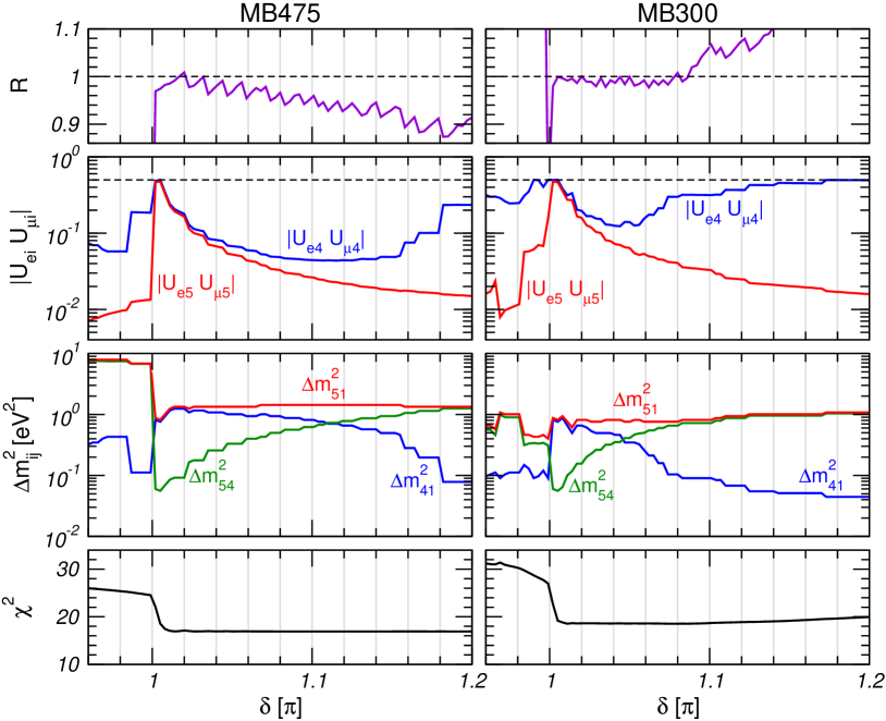
Figure 52: Fit to appearance data LSND, KARMEN, NOMAD, and MB475 (left) or MB300 (right) in (3+2) schemes. We show the $\chi^{2}$, the mass splittings $\Delta m^{2}_{i1}$, the mixing angles $|U_{ei}U_{\mu i}|$ and the ratio $R=\big{(}|U_{e4}U_{\mu 4}|\Delta m^{2}_{41}\big{)}\,\big{/}\,\big{(}|U_{e5}U_{\mu 5}|\Delta m^{2}_{51}\big{)}$ as a function of the complex phase $\delta$ defined in Eq. (332). Adapted from Ref. [380].

Let us now turn to the issue of reconciling MiniBooNE with LSND. First of all, note that the condition (334) suppresses $P_{\nu_{\mu}\to\nu_{e}}$ at high energies for both neutrinos and antineutrinos. At lower energies a non-trivial way to keep this probability small can be obtained by requiring $\cos(\phi_{54}-\delta)=-1$. Then one has

$$P_{\nu_{\mu}\to\nu_{e}}=4\left(|U_{e4}U_{\mu 4}|\sin\phi_{41}-|U_{e5}U_{\mu 5}|\sin\phi_{51}\right)^{2}\,,\quad\cos(\phi_{54}-\delta)=-1\,.$$ (335)

Hence, $P_{\nu_{\mu}\to\nu_{e}}$ is small for $|U_{e4}U_{\mu 4}|\approx|U_{e5}U_{\mu 5}|$ and $\phi_{54}\ll 1$. This is precisely the behavior shown in Fig. 52: when $\delta$ approaches $\pi$ from above, $\Delta m^{2}_{54}$ becomes small and the $|U_{ei}U_{\mu i}|$ approach each other. Writing $\delta=\pi+\epsilon$ one has $\cos(\phi_{54}-\delta)\approx-1+\mathcal{O}(\phi_{54}^{2},\,\epsilon^{2})$, Eq. (335) is valid, and the oscillation probability is suppressed in MB. Now the question arises whether large enough values for $P_{\bar{\nu}_{\mu}\to\bar{\nu}_{e}}$ can be achieved in order to explain LSND. The difference of anti-neutrino and neutrino probabilities is given by

$$\begin{split}P_{\bar{\nu}_{\mu}\to\bar{\nu}_{e}}-P_{\nu_{\mu}\to\nu_{e}}&=16\,|U_{e4}\,U_{\mu 4}\,U_{e5}\,U_{\mu 5}|\,\sin\phi_{41}\,\sin\phi_{51}\,\sin\phi_{54}\,\sin\epsilon\\[2.84526pt] &\approx 16\,|U_{e4}\,U_{\mu 4}\,U_{e5}\,U_{\mu 5}|\,\sin^{2}(\phi_{51})\,\phi_{54}\epsilon\,,\end{split}$$ (336)

where in the last step $\phi_{54},\epsilon\ll 1$ has been used. Since $\phi_{54}$ and $\epsilon$ are small, the other factors have to be as large as possible in order to get a sufficient probability for LSND. Indeed, for $\Delta m^{2}_{51}\approx 1$ eV² one has $\sin^{2}\phi_{51}\approx 1$, and also $|U_{ei}\,U_{\mu i}|$ grow for $\epsilon\to 0$ (see Fig. 52). Once the maximal values allowed by unitarity, $|U_{e4}\,U_{\mu 4}|=|U_{e5}\,U_{\mu 5}|=1/2$, are reached the LSND probability is given roughly by $P_{\bar{\nu}_{\mu}\to\bar{\nu}_{e}}\sim 4\epsilon^{2}$, where we used $P_{\nu_{\mu}\to\nu_{e}}\approx 0$ (in order to explain MB) and $\phi_{54}\approx\epsilon$ (in order to have $\cos(\phi_{54}-\delta)\approx-1$). Using the experimental value $P_{\mathrm{LSND}}=0.0026$ one finds that a fit should be possible for $\epsilon\gtrsim 0.025\approx 0.008\pi$, in agreement with our results.

The similar structure of the left and right panels of Fig. 52 suggests that this mechanism works equally well for MB475 and MB300, and fitting the low energy excess in MB does not affect these considerations. Obviously, this explanation is not valid for $\delta<\pi$, since the CP asymmetry Eq. (336) has the wrong sign to reconcile LSND and MB. As visible in Fig. 52, the fit jumps into a quite different solution, which anyway gives a poor $\chi^{2}$.

Concerning the constraints from disappearance experiments, in the (3+2) schemes the relevant survival probability in the SBL approximation is given

$$P_{\nu_{\alpha}\to\nu_{\alpha}}=1-4\left(1-\sum_{i=4,5}|U_{\alpha i}|^{2}\right)\sum_{i=4,5}|U_{\alpha i}|^{2}\,\sin^{2}\phi_{i1}\\ -4\,|U_{\alpha 4}|^{2}|U_{\alpha 5}|^{2}\,\sin^{2}\phi_{54}$$ (337)

where $\phi_{ij}$ is given in Eq. (332). Similar as in the (3+1) case, also for (3+2) schemes atmospheric neutrino data provide an important constraint on $\nu_{\mu}$ oscillations with sterile neutrinos. It turns out that in practice the same constraint $\chi^{2}_{\mathrm{ATM}}(d_{\mu})$ as in the four-neutrino case applies (see the right panel of Fig. 50), where now the definition $d_{\mu}=|U_{\mu 4}|^{2}+|U_{\mu 5}|^{2}$ has to be used.

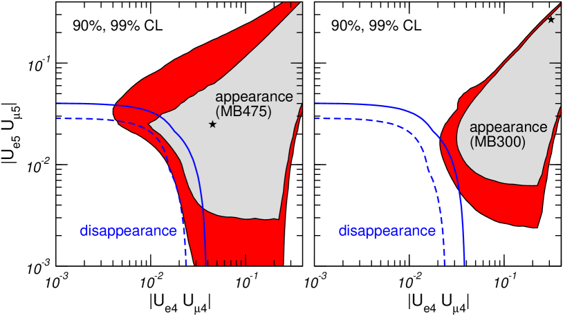
Figure 53: Allowed regions at 90% and 99% CL in (3+2) schemes for appearance data (shaded regions) and disappearance data (dashed and solid curves) projected onto the plane of $|U_{e4}U_{\mu 4}|$ and $|U_{e5}U_{\mu 5}|$. In the left panel the two lowest energy data points in MB have been omitted (MB475), whereas in the right panel the full MB energy range has been used in the fit (MB300). Taken from Ref. [380].

As discussed above, and clearly shown in Table 6, rather large values of $|U_{e4}\,U_{\mu 4}|$ and $|U_{e5}\,U_{\mu 5}|$ are needed in order to reconcile the negative result of MiniBooNE with the positive signal of LSND. This is particularly true when the full MB300 data set is used. However, even in (3+2) schemes short-baseline experiments pose stringent bounds on the mixing angles $|U_{ei}|$ and $|U_{\mu i}|$, in close analogy with (3+1) models described in Sec. 9.1.1. Therefore, one expects that reconciling appearance and disappearance data will be a problem also within (3+2) models. This tension is illustrated in Fig. 53, where the projections of the allowed regions in the plane of the appearance amplitudes $|U_{e4}U_{\mu 4}|$ and $|U_{e5}U_{\mu 5}|$ are shown. Indeed the opposite trend of the two data sets is clearly visible, especially when the low energy excess in MB is included (right panel).

In order to quantify the disagreement between appearance and disappearance data, one can aply the PG test described in [381] using the $\chi^{2}_{\text{PG}}$ values, for global data without MB, with MB475, and with MB300:

$$\chi^{2}_{\text{PG}} =17.5\,,\quad =1.5\times 10^{-3}\qquad\text{(no MB)}$$ PG (338)

$$\mbox{APP vs DIS:}\qquad\chi^{2}_{\text{PG}} =17.2\,,\quad =1.8\times 10^{-3}\qquad\text{(MB475)}$$ PG

$$\chi^{2}_{\text{PG}} =25.1\,,\quad =4.8\times 10^{-5}\qquad\text{(MB300)}$$ PG

From these numbers one can conclude that also in (3+2) schemes the tension between appearance and disappearance experiments is quite severe. If MB475 is used the result is very similar to the situation without MB data implying inconsistency at about $3.1\sigma$, whereas in case of the full MB300 data the tension becomes significantly worse (about $4\sigma$), since appearance data are more constraining because of the need to accommodate LSND as well as the MB excess at low energies.

9.2.2 (3+3) six-neutrino mass schemes

Since there are three active neutrinos it seems natural to consider also the case of three sterile neutrinos. If all three additional neutrino states have masses in the eV range and mixings as relevant for the SBL experiments under consideration, such a model will certainly have severe difficulties to accommodate standard cosmology [387, 388], and one has to refer to some non-standard cosmological scenario [389, 390, 391, 392, 393, 394].

Besides this fact, the results of the search performed in Ref. [380] show that there is only a marginal improvement of the fit (by 1.7 units in $\chi^{2}$) for MB475 (3.5 for MB300) with respect to (3+2), to be compared with 4 additional parameters in the model. Hence, the conclusion is that that there are no qualitatively new effects in the (3+3) scheme. The conflict between appearance and disappearance data remains a problem, and the additional freedom introduced by four new parameters does not relax significantly this tension.

9.3 Violation of CPT

In Ref. [395] it was observed that the LSND signal could be accommodated with the solar and atmospheric neutrino anomalies without enlarging the neutrino sector if CPT was violated. Once such a drastic modification of standard physics is accepted, oscillations with four independent $\Delta m^{2}$ are possible, two in the neutrino and two in the anti-neutrino sector. The basic realization behind these proposals is that the oscillation interpretation of the solar results involves oscillations of electron neutrinos with $\Delta m^{2}_{\odot}\lesssim 10^{-4}~{}\text{eV}^{2}$ while the LSND signal for short baseline oscillations with $\Delta m^{2}_{\text{LSND}}\gtrsim 10^{-1}~{}\text{eV}^{2}$ stems dominantly from anti-neutrinos ($\bar{\nu}_{\mu}\to\bar{\nu}_{e}$). If CPT was violated and neutrino and anti-neutrino mass spectra and mixings were different [395, 396, 397, 398, 399] both results could be made compatible in addition to the interpretation of the atmospheric neutrino data in terms of oscillations of both $\nu_{\mu}$ and $\bar{\nu}_{\mu}$ with $\Delta m^{2}_{\text{atm}}\sim 10^{-3}~{}\text{eV}^{2}$.

Notice that, in principle, these scenarios could accommodate both the evidence of LSND and the negative results of MiniBooNE obtained running in the neutrino mode, as the neutrino spectrum may not oscillate with the large $\Delta m^{2}$ while the antineutrino does. For this scenarios the data from MiniBooNE running in the antineutrino mode will be most relevant.

In the original spectrum proposed, neutrinos had mass splittings $\Delta m^{2}_{\odot}=\Delta m^{2}_{21}\ll\Delta m^{2}_{31}=\Delta m^{2}_{\text{atm}}$ to explain the solar and atmospheric observations, while for anti-neutrinos $\Delta m^{2}_{\text{atm}}=\Delta\bar{m}^{2}_{21}\ll\Delta\bar{m}^{2}_{31}=\Delta m^{2}_{\text{LSND}}$. Within this spectrum the mixing angles could be adjusted to obey the relevant constraints from laboratory experiments, mainly due to the non-observation of reactor $\bar{\nu}_{e}$ at short distances and a reasonable description of the data could be achieved [399, 400, 401]. In general, stronger constraints on the possibility of CPT violation arise, once a specific source of CPT violation which involves other sectors of the theory is invoked [402, 403].

On pure phenomenological grounds, the first test of this scenario came from the KamLAND experiment since the suggested CPT-violating neutrino spectrum allowed to reconcile the solar, atmospheric and LSND anomalies, but, once the constraints from reactor experiments were imposed, no effect in KamLAND was predicted. The observation of a deficit in KamLAND at $3.5\sigma$ CL clearly disfavored these scenarios. Furthermore, KamLAND results demonstrate that $\bar{\nu}_{e}$ oscillate with parameters consistent with the LMA $\nu_{e}$ oscillation solution of the solar anomaly. This fact by itself can be used to set constraints on the possibility of CPT violation [404, 401].

The present situation is that the results of solar experiments in $\nu$ oscillations, together with the results from KamLAND and the bounds from other $\bar{\nu}$ reactor experiments show that both neutrinos and anti-neutrinos oscillate with $\Delta m^{2}_{\odot},\,\Delta m^{2}_{\text{reac}}\leq 10^{-3}~{}\text{eV}^{2}$. Adding this to the evidence of oscillations of both atmospheric neutrinos and anti-neutrinos with $\Delta m^{2}_{\text{atm}}\sim 10^{-3}~{}\text{eV}^{2}$, leaves no room for oscillations with $\Delta m^{2}_{\text{LSND}}\sim 1~{}\text{eV}^{2}$. The obvious conclusion then is that CPT violation could no-longer explain LSND and perfectly fit all other data [401].

This conclusion relies strongly on the fact that atmospheric oscillations have been observed for both neutrinos and anti-neutrinos with the same $\Delta m^{2}_{\text{atm}}$. However atmospheric neutrino experiments do not distinguish neutrinos from anti-neutrinos, and neutrinos contribute more than anti-neutrinos to the event rates by a factor $\sim$ 4–2 (the factor decreases for higher energies). Based on this fact, in Refs. [398, 401] an alternative CPT-violating spectrum was proposed as shown in Fig. 54. In this scheme only atmospheric neutrinos oscillate with $\Delta m^{2}_{\text{atm}}$ and give most of the contribution to the observed zenith angular dependence of the deficit of $\mu$-like events. Atmospheric $\bar{\nu}_{\mu}$ dominantly oscillate with $\Delta m^{2}_{\text{LSND}}$ which leads to an almost constant (energy and angular independent) suppression of the corresponding events. For low $\bar{\nu}_{\mu}$ energies oscillations with $\Delta m^{2}_{\text{reac}}$ can also be a source of zenith-angular dependence. The claim in Ref. [398] was that altogether this suffices to give a good description of the atmospheric data such that the scheme in Fig. 54 could still be a viable solution to all the neutrino puzzles. This conclusion was contradicted in Ref. [401] by an analysis of atmospheric and K2K data. However, according to the authors in Ref. [398] an important point to their conclusion was the consideration of the full $3\nu$ and $3\bar{\nu}$ oscillations, while the analysis in Ref. [401] was made on the basis of a $2\nu+2\bar{\nu}$ approximation.

Figure 54: Post KamLAND CPT violating neutrino mass spectrum proposed in Ref. [398].

In Ref. [405] the status of the CPT violating scenario in Fig. 54 as explanation to the existing neutrino anomalies was revisited and we summarize and update here their main conclusions.

One can label the states as in Fig. 54 with $\Delta m^{2}_{ij}=m^{2}_{i}-m^{2}_{j}$ and $\Delta\bar{m}^{2}_{ij}=\bar{m}^{2}_{i}-\bar{m}^{2}_{j}$ and denote by $U$ and $\bar{U}$ the corresponding neutrino and anti-neutrino mixing matrix (neglecting CP phases).

In the anti-neutrino sector the most constraining results of $\bar{\nu}_{e}$ mixing comes from KamLAND, Bugey and CHOOZ. They provide information on the $\bar{\nu}_{e}$ survival probability:

$$\begin{split}P_{ee}^{\text{reac}}&=1-\bar{c}_{13}^{4}\,\sin^{2}2\bar{\theta}_{12}\,\sin^{2}\left(\frac{\Delta\bar{m}^{2}_{21}L}{4E}\right)\\ &\hskip 14.22636pt\sin^{2}2{\bar{\theta}_{13}}\left[\bar{c}_{12}^{2}\,\sin^{2}\left(\frac{\Delta\bar{m}^{2}_{31}L}{4E}\right)+\bar{s}_{12}^{2}\,\sin^{2}\left(\frac{\Delta\bar{m}^{2}_{32}L}{4E}\right)\right]\\[8.53581pt] &\simeq\begin{cases}1-\sin^{2}2\bar{\theta}_{13}\sin^{2}\left(\dfrac{\Delta\bar{m}^{2}_{31}L}{4E}\right)&\text{for}\quad\Delta\bar{m}^{2}_{21}L/E\ll 1\\[11.38109pt] \bar{s}_{13}^{4}+\bar{c}_{13}^{4}\left[1-\sin^{2}2\bar{\theta}_{12}\,\sin^{2}\left(\dfrac{\Delta\bar{m}^{2}_{21}L}{4E}\right)\right]&\text{for}\quad\Delta\bar{m}^{2}_{31}L/E\gg 1\end{cases}\end{split}$$ (339)

In the scheme under consideration the probability associated with the $\bar{\nu}_{\mu}\to\bar{\nu}_{e}$ signal in LSND is given by

$$P_{\text{LSND}}\equiv\sin^{2}2\theta_{\text{LSND}}\sin^{2}\left(\frac{\Delta m^{2}_{\text{LSND}}L}{4E}\right)=\bar{s}_{23}^{2}\sin^{2}2\bar{\theta}_{13}\,\sin^{2}\left(\frac{\Delta\bar{m}^{2}_{31}L}{4E}\right)\,,$$ (340)

where terms proportional to $\Delta\bar{m}^{2}_{21}$ which are irrelevant for LSND distances and energies have been neglected. In Eq. (340):

$$\Delta m^{2}_{\text{LSND}}=\Delta\bar{m}^{2}_{31}\,,\qquad\sin^{2}2\theta_{\text{LSND}}=\bar{s}_{23}^{2}\,\sin^{2}2\bar{\theta}_{13}\,.$$ (341)

For the neutrino sector relevant information arises from solar neutrino experiments and the K2K and MINOS LBL experiments. The relevant probabilities are given in Eq. (95) for solar neutrinos and Eq. (98) for K2K and MINOS.

Finally, the analysis of atmospheric neutrino data involves oscillations of both neutrinos and anti-neutrinos, and, in the framework of $3\nu+3\bar{\nu}$ mixing, matter effects become relevant and its effect has to be quantified by numerically solving the evolution equations for neutrinos and antineutrinos.

The basic approach to test the status of the scheme in Fig. 54 as a possible explanation of the LSND anomaly together with all other neutrino and anti-neutrino oscillation data is as follows. First, one performs a global analysis of all the relevant data, but leaving out LSND data. The goal of this analysis is to obtain the allowed ranges of parameters $\Delta m^{2}_{\text{LSND}}$ and $\sin^{2}2\theta_{\text{LSND}}$ as defined in Eq. (341) from this all-but-LSND data set. Then one compares these allowed regions to the corresponding allowed parameter region from LSND, and quantify at which CL both regions become compatible.

In this approach one starts by defining the most general $\chi^{2}$ for the all-but-LSND data set:

$$\chi^{2}_{\text{all-but-LSND}}(\Delta m^{2}_{21},\Delta m^{2}_{31},\theta_{12},\theta_{13},\theta_{23}\,|\,\Delta\bar{m}^{2}_{21},\Delta\bar{m}^{2}_{31},\bar{\theta}_{12},\bar{\theta}_{13},\bar{\theta}_{23})=\\ \chi^{2}_{\text{solar}}(\Delta m^{2}_{21},\theta_{12},\theta_{13})+\chi^{2}_{\text{K2K+MINOS}}(\Delta m^{2}_{31},\theta_{23},\theta_{13})\\ +\chi^{2}_{\text{Bugey+CHOOZ+KLAND}}(\Delta\bar{m}^{2}_{21},\Delta\bar{m}^{2}_{31},\bar{\theta}_{12},\bar{\theta}_{13})\\ +\chi^{2}_{\text{atmos}}(\Delta m^{2}_{21},\Delta m^{2}_{31},\theta_{12},\theta_{23},\theta_{13}\,|\,\Delta\bar{m}^{2}_{21},\Delta\bar{m}^{2}_{31},\bar{\theta}_{12},\bar{\theta}_{23},\bar{\theta}_{13})\,.$$ (342)

In order to test the status of the CPT interpretation of the LSND signal using data independent of the “tension” between LSND and KARMEN results [406] the constraints from the non-observation of $\bar{\nu}_{\mu}\to\bar{\nu}_{e}$ transitions at KARMEN have not been included.

Using all the data described above except from the LSND experiment we find the following all-but-LSND best fit point:

$$\;\Delta m^{2}_{21} =6.8\times 10^{-5}~{}\text{eV}^{2}\,,\qquad \;\Delta\bar{m}^{2}_{21} =7.6\times 10^{-5}~{}\text{eV}^{2}\,,$$ (343)

$$|\Delta m^{2}_{31}| =2.4\times 10^{-3}~{}\text{eV}^{2}\,,\qquad |\Delta\bar{m}^{2}_{31}| =2.2\times 10^{-3}~{}\text{eV}^{2}\,,$$

$$\sin^{2}\theta_{12} =0.30\,,\qquad \sin^{2}\bar{\theta}_{12} =0.36\,,$$

$$\sin^{2}\theta_{13} =0\,,\qquad \sin^{2}\bar{\theta}_{13} =0\,,$$

$$\sin^{2}\theta_{23} =0.5\,,\qquad \sin^{2}\bar{\theta}_{23} =0.5\,.$$

This can be directly compared to the corresponding analysis in the CPT conserving scenario:

$$\;\Delta m^{2}_{21}\;=\;\Delta\bar{m}^{2}_{21} =7.7\times 10^{-5}~{}\text{eV}^{2}\,,$$ (344)

$$|\Delta m^{2}_{31}|=|\Delta\bar{m}^{2}_{31}| =2.4\times 10^{-3}~{}\text{eV}^{2}\,,$$

$$\sin^{2}\theta_{12}=\sin^{2}\bar{\theta}_{12} =0.32\,,$$

$$\sin^{2}\theta_{13}=\sin^{2}\bar{\theta}_{13} =0\,,$$

$$\sin^{2}\theta_{23}=\sin^{2}\bar{\theta}_{23} =0.5\,.$$

Thus allowing for different mass and mixing parameters for neutrinos and anti-neutrinos, all-but-LSND data choose a best fit point very close to CPT conservation and maximal $23$ mixing.

Figure 55: Allowed regions for neutrino and anti-neutrino mass splittings and mixing angles in the CPT violating scenario. Different contours correspond to the two-dimensional allowed regions at 90%, 95%, 99% and $3\sigma$ CL. The best fit point is marked with a star.

Next we illustrate the amount of CPT violation which is still viable. In order to do so we plot in Fig. 55 the allowed regions for the neutrino and anti-neutrino mass splittings and mixing angles. From the figure we find that present data constraints all mixing angles and absolute values of mass-squared differences to be close to the CPT conserving case. However, as seen in the four lower left panels, nothing is known about the relative ordering of neutrinos versus antineutrino states. CPT scenarios in which neutrinos states are normally ordered while antineutrino states are inversely ordered (or vice-versa) cannot be discriminated from the CPT conserving case.

Concerning LSND, the results show that values of $\Delta\bar{m}^{2}_{31}=\Delta\bar{m}^{2}_{\text{LSND}}$ large enough to fit the LSND result do not appear as part of the $3\sigma$ CL allowed region of the all-but-LSND analysis which is bounded to $\Delta\bar{m}^{2}_{31}<0.01~{}\text{eV}^{2}$. The upper bound on $\Delta\bar{m}^{2}_{31}$ is determined by atmospheric neutrino data. It is clear from these results that the CPT violation scenario cannot give a good description of the LSND data and simultaneously fit all-but-LSND results. The quantification of this statement is displayed in Fig. 56 where we show the allowed regions in the ($\Delta\bar{m}^{2}_{31}=\Delta m^{2}_{\text{LSND}}$, $\sin^{2}2\theta_{\text{LSND}}$) plane required to explain the LSND signal together with the corresponding allowed regions from the global analysis of all-but-LSND data.

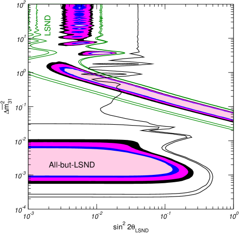
Figure 56: 90%, 95%, 99%, and $3\sigma$ CL allowed regions (filled) in the ($\Delta\bar{m}^{2}_{31}=\Delta m^{2}_{\text{LSND}}$, $\sin^{2}2\theta_{\text{LSND}}$) plane required to explain the LSND signal together with the corresponding allowed regions from our global analysis of all-but-LSND data. The contour lines correspond to $\Delta\chi^{2}=26$ and $30$ ($4.7\sigma$ and $5.1\sigma$, respectively).

Fig. 56 illustrates that below $3\sigma$ CL there is no overlap between the allowed region of the LSND analysis and the all-but-LSND one, and that for this last one the region is restricted to $\Delta\bar{m}^{2}_{31}=\Delta m^{2}_{\text{LSND}}<0.01~{}\text{eV}^{2}$. Only for $\Delta\chi^{2}\gtrsim 25$ values of $\Delta\bar{m}^{2}_{31}\sim\mathcal{O}(\text{eV}^{2})$ become allowed for the all-but-LSND region – as determined mainly by the constraints from Bugey – and at the $4.6\sigma$ level ($\chi^{2}_{\text{PC}}=25.2$) an agreement with LSND becomes possible.

The information most relevant to this conclusion comes from the atmospheric neutrino events. Within the constraints imposed by solar and LBL neutrino data, and reactor anti-neutrino experiments, atmospheric data is precise enough to be sensitive to anti-neutrino oscillation parameters and cannot be described with oscillations with the wavelengths required in the CPT violating scenario.

9.4 Other Extensions

Further extensions of the $3\nu$ mixing scenario have been proposed in the literature with the aim of accommodating the LSND observation [407, 408, 409, 410, 411, 412, 413]. We briefly summarize the basic features of some of these proposals.

In Ref. [407] it is examined the possibility that a four-neutrino scenario with $CPT$ violation can explain the LSND effect and remain consistent with all other data. The authors find that models with a (3+1) mass structure in the neutrino sector are viable with the third mass difference between $1-7~{}\text{eV}^{2}$ while a (2+2) structure is permitted only in the antineutrino sector and the third mass difference can extend to all the ranges allowed by LSND, KARMEN and Bugey. The non-observation of a signature at MiniBooNE in the neutrino channel cannot rule out any of these models. The observation or non-observation of a signal in MiniBooNE in the antineutrino mode could discriminate between these two scenarios.

The proposal that mass-varying neutrinos could provide an explanation for the LSND signal for $\bar{\nu}_{\mu}\to\bar{\nu}_{e}$ oscillations was studied in Ref. [408]. It is based on the observation of Ref. [224] that all positive oscillation signals mostly occur in matter and therefore if there is a contribution to the neutrino mass depending on the matter density, the effective mass differences in the different experiments can be different, a fact that can help in accommodating the LSND results. They find that three active mass-varying neutrinos are insufficient to describe all existing neutrino data including LSND. But mass-varying neutrinos with a (3+1) mass structure in the neutrino sector can work with a small active-sterile mixing which is generated solely by MaVaN effects. These scenarios predict a null MiniBooNE (and are therefore still viable), a null result at Double-CHOOZ, but positive signals for underground reactor experiments and for $\nu_{\mu}\to\nu_{e}$ oscillations in long-baseline experiments.

Explanations of the LSND evidence for electron antineutrino appearance based on neutrino decay have been also studied in the literature [409, 410]. In the most updated of this proposals [410] a fourth heavier sterile neutrino is introduced with a (3+1) mass structure. Such neutrino is produced in pion and muon decays because of a small mixing with muon neutrinos, and then decays into a scalar particle and a light neutrino, predominantly of the electron type giving the observed signature at LSND. The basic point is that the different $L/E$ dependence of the flavor conversion probabilities for this scenario compared to the oscillation case allows for a larger range of compatibility between the LSND observation and the null result at KARMEN and other SBL experiments. In the minimal version, this decay model predicted a signal in the MiniBooNE experiment corresponding to a transition probability of the same order as seen in LSND and it is therefore disfavored by the negative result of MiniBooNE. However, in Ref. [410] it was noted that the inclusion of a second sterile neutrino would open up the possibility of CP-violating effects, in a similar way to what discussed in Sec. 9.2, hence potentially allowing to reconcile LSND and MiniBooNE.

The possibility of a new resonance in active-sterile neutrino oscillations arising in theories with large extra dimensions is studied in Ref. [411]. In these scenarios the fluctuations in the brane effectively increase the path-length of active neutrinos relative to the path-length of sterile neutrinos through the extra-dimensional bulk. This imparts an energy dependence to the oscillation amplitude which can lead to the resonant enhancement of active-sterile neutrino mixing. For energies below the resonance, the flavor conversion probabilities take the standard oscillation form while above the resonance, active-sterile oscillations are suppressed. The authors find that if the resonant energy lies in the range 30 MeV to 400 MeV, suitably chosen between the BUGEY and CDHS energies, then all neutrino oscillation data can be accommodated in a consistent (3+1) neutrino framework. Such an energy range corresponds to brane fluctuations with a height to width ratio of $\sim 10^{-8}$. The resonant energy might be identifiable in either the LSND spectral data and the muon neutrino disappearance from a stopped-pion source, or, as a matter of fact, in the MiniBooNE data itself.

In Ref. [414] it was postulated the existence of Lorentz-violating, CPT-conserving interactions which could allow three-neutrino solutions to the LSND anomaly that are also consistent with all other neutrino data. They found that a highly non-trivial energy dependence of the Lorentz-violating interactions is required to accommodate all the data. The non observation of a signal at MiniBooNE imposes even stronger constrains on the energy dependence of these interactions.

10 Summary and Conclusions

In this review we have presented the progress on some fronts of the phenomenology of massive neutrinos. The present experimental situation concerning the searches for neutrino flavor mixing with respectively, solar, atmospheric, reactor and accelerator neutrinos was presented in Sec. 2. From this data we have learned that:

• Solar $\nu_{e}^{\prime}s$ convert to $\nu_{\mu}$ or $\nu_{\tau}$ with confidence level (CL) of more than $7\sigma$.

• KamLAND find that reactor $\bar{\nu}_{e}$ disappear over distances of about 180 km and they observe a distortion of their energy spectrum. Altogether their evidence has more than $3\sigma$ CL.

• The evidence of atmospheric (ATM) $\nu_{\mu}$ disappearing is now at $>15\sigma$, most likely converting to $\nu_{\tau}$.

• K2K observe the disappearance of accelerator $\nu_{\mu}$’s at distance of 250 km and find a distortion of their energy spectrum with a CL of 2.5–4$\sigma$.

• MINOS observes the disappearance of accelerator $\nu_{\mu}$’s at distance of 735 km and find a distortion of their energy spectrum with a CL of $\sim 5\sigma$.

• LSND found evidence for $\bar{\nu}_{\mu}\rightarrow\bar{\nu}_{e}$. This evidence has not been confirmed by the recent MiniBooNE search for $\nu_{\mu}\rightarrow\nu_{e}$ at 98% CL.

These results imply that neutrinos are massive and the Standard Model has to be extended at least to include neutrino masses.

In Sec. 1 we have presented the low energy formalism for adding neutrino masses to the SM which would allow for the observed leptonic mixing and we have described the phenomenology associated with neutrino oscillations in vacuum and in matter needed for the interpretation of the data.

The minimum joint description of solar, atmospheric, long baseline and reactor data requires the mixing of the three known neutrinos. In Sec. 3 we have presented an update of the three-neutrino oscillation interpretation of the existing bulk of neutrino data (with the exception of the LSND result). The derived ranges for the two mass differences at $1\sigma$ ($3\sigma$) are:

$$\Delta m^{2}_{21} =7.67\,_{-0.21}^{+0.22}\,\left({}_{-0.61}^{+0.67}\right)\times 10^{-5}~{}\text{eV}^{2}\,,$$ (345)

$$\Delta m^{2}_{31} =\begin{cases}-2.37\pm 0.15\,\left({}_{-0.46}^{+0.43}\right)\times 10^{-3}~{}\text{eV}^{2}&\text{(inverted hierarchy)}\,,\\[2.84526pt] +2.46\pm 0.15\,\left({}_{-0.42}^{+0.47}\right)\times 10^{-3}~{}\text{eV}^{2}&\text{(normal hierarchy)}\end{cases}$$

while the leptonic mixing matrix at the $3\sigma$ level is:

$$|U|_{3\sigma}=\begin{pmatrix}0.77\to 0.86&~{}\quad~{}0.50\to 0.63&~{}\quad~{}0.00\to 0.22\\ 0.22\to 0.56&~{}\quad~{}0.44\to 0.73&~{}\quad~{}0.57\to 0.80\\ 0.21\to 0.55&~{}\quad~{}0.40\to 0.71&~{}\quad~{}0.59\to 0.82\end{pmatrix}\,.$$ (346)

This minimal picture of three massive neutrinos, although can give a satisfactory description of the data is still incomplete. We have no direct evidence of the mixing angle $\theta_{13}$, we ignore if CP is a symmetry of the leptonic sector, we do not know the ordering of the mass states, and most importantly we do not know if neutrinos are Majorana or Dirac particles.

Also, although oscillations have allowed us to establish that neutrinos have mass they only provide a lower bound on the heaviest neutrino mass, but give no information on the mass of the lightest state which sets the absolute neutrino mass scale. As described in Sec. 8 at present, the most precise and model independent bound on scale of neutrino masses still arises from the non observation of any distortion at the end-point of the energy spectrum of the electrons emitted in tritium beta decay which imply that $\sqrt{\sum_{i}m^{2}_{i}|U_{ei}|^{2}}<2.2~{}\text{eV}$ at 95% confidence level.

We have argued and show how, despite all these limitations, the attained precision in the observed signals is already good enough to allow us the use of the existing data to probe physics beyond neutrino masses and mixing. In Sec. 4 we have shown how the independent determination of the relevant neutrino oscillation parameters from non-solar and non-atmospheric neutrino experiments makes it possible to extract the solar and atmospheric neutrino fluxes directly from the corresponding neutrino data with an accuracy comparable, to that of the theoretical predictions from the solar model and from atmospheric flux calculations.

Using the good description of neutrino data in terms of neutrino oscillations, it is also possible to constraint other exotic forms of new physics as shown in Secs. 5 and 6. We have presented updated bounds on the violation of some fundamental symmetries like Lorentz Invariance, the Equivalence Principle and CPT. These forms of new physics, if non-universal, can also induce neutrino flavor oscillations whose main differentiating characteristic is a different energy dependence of the oscillation wavelength. We have also discussed the present constraints on the presence of non-standard neutrino interactions affecting the solar and atmospheric neutrino propagation in matter as well as on effects associated with mass varying neutrinos models. Under certain assumptions these results represent the most stringent bounds on these forms of new physics.

Another hint for neutrino masses came from the LSND experiment. The simplest interpretation of the LSND data is that there are $\nu_{e}\to\nu_{\mu}$ oscillations with $\Delta m^{2}_{\text{LSND}}=\mathcal{O}(1~{}\text{eV}^{2})$ and $\sin^{2}2\theta_{\text{LSND}}=\mathcal{O}(0.003)$.

The fact that $\Delta m^{2}_{\text{LSND}}\gg\Delta m^{2}_{31},\,\Delta m^{2}_{21}$ means that this result cannot be included within the framework of oscillations among the three active neutrinos alone. Therefore a further extension of the SM model is needed. We present in Sec. 9 the updated status of some extensions including a fourth sterile neutrino or three neutrinos with violation of CPT symmetry. The conclusion is that these extensions are either ruled out or strongly disfavor as possible explanations of the LSND signal.

At the time of the finishing of this review the results of the MiniBooNE experiment, which was especially designed to make a conclusive statement about the LSND’s neutrino oscillation evidence, were made public. In their search for $\nu_{\mu}\to\nu_{e}$ they found no evidence of the expected signal corresponding to the LSND evidence, thus excluding the LSND claim at 98% CL in the 2-$\nu$ oscillation framework. This result puts further constrains on the possible mixings of an additional sterile neutrino, while in principle could be accommodated together with the LSND evidence if CPT was violated. However CPT violation is independently excluded well beyond $3\sigma$ as explanation to the LSND data because (i) KamLAND finds that reactor $\bar{\nu}_{e}$ oscillate with wavelength and amplitude in good agreement with the expectations from the LMA solution of the solar $\nu_{e}$, and (ii) both ATM neutrinos and antineutrinos have to oscillate with similar wavelengths and amplitudes to explain the ATM data.

In summary, neutrino physics has provided us with the first evidence of physics beyond the standard model, it has allowed us to test many theoretical ideas and given experimental guidance in the construction of new ones. But many questions remain open and the only way to answer them is by new experiments, some of which are, fortunately, on the way.

Appendix A Atmospheric Neutrino Analysis

In this appendix we describe and update the details entering into the simulation of the atmospheric neutrino event rates of Super-Kamiokande used in the analysis presented in this review as well as the corresponding statistical treatment.

A.1 Event Rates

Underground experiments can record atmospheric neutrinos by direct observation of their charged current interaction inside the detector. These so-called contained events can be classified into fully contained events, when the charged lepton (either electron or muon) produced by the neutrino interaction does not escape the detector, and partially contained muons, when a muon is produced inside but then leaves the detector. In the simulation of Super–Kamiokande used in this review the fully contained events are further divided into three data samples, based on the energy of the charged lepton:

• $\text{sub-GeV}_{\text{low}}$, with lepton momentum below 400 MeV;

• $\text{sub-GeV}_{\text{high}}$, with higher lepton momentum but visible energy below 1.33 GeV;

• multi-GeV, with visible energy above this cutoff.

In addition, both fully and partially contained events are also divided into 10 zenith bins, based on the reconstructed direction of the charged lepton. Thus in this simulation there id a total of 70 data bins for contained events.

The expected number of events in each bin can be obtained as:

$$N_{\text{bin}}(\vec{\omega})=n_{t}T\sum_{\alpha,\beta,\pm}\int_{0}^{\infty}dh\int_{-1}^{+1}dc_{\nu}\int_{E_{\text{min}}}^{\infty}dE_{\nu}\int_{E_{\text{min}}}^{E_{\nu}}dE_{l}\int_{-1}^{+1}dc_{a}\int_{0}^{2\pi}d\varphi_{a}\\ \frac{d^{3}\Phi_{\alpha}^{\pm}}{dE_{\nu}\,dc_{\nu}\,dh}(E_{\nu},c_{\nu},h)\,P_{\alpha\to\beta}^{\pm}(E_{\nu},c_{\nu},h\,|\,\vec{\omega})\,\left[\frac{d^{2}\sigma_{\beta}^{\pm}}{dE_{l}\,dc_{a}}\,\pi_{\text{ring}}\right](E_{\nu},E_{l},c_{a})\\ \times\varepsilon_{\beta}^{\text{bin}}(E_{l},c_{l}(c_{\nu},c_{a},\varphi_{a}))\,,$$ (347)

where $P_{\alpha\to\beta}^{+}$ ($P_{\alpha\to\beta}^{-}$) is the $\nu_{\alpha}\to\nu_{\beta}$ ($\bar{\nu}_{\alpha}\to\bar{\nu}_{\beta}$) conversion probability for given values of the neutrino energy $E_{\nu}$, the cosine $c_{\nu}$ of the angle between the incoming neutrino and the vertical direction, and the production altitude $h$. In the Standard Model one has $P_{\alpha\to\beta}^{\pm}=\delta_{\alpha\beta}$ for all $\alpha$ and $\beta$, whereas when neutrino oscillations are considered the expression for $P_{\alpha\to\beta}^{\pm}$ depends also on the conversion model and on its parameters $\vec{\omega}$. In Eq. (347) $n_{t}$ is the number of targets, $T$ is the experiment running time, $\Phi_{\alpha}^{+}$ ($\Phi_{\alpha}^{-}$) is the flux of atmospheric neutrinos (antineutrinos) of type $\alpha$ and $\sigma_{\beta}^{+}$ ($\sigma_{\beta}^{-}$) is the charged-current neutrino- (antineutrino-) nucleon interaction cross section. The variable $E_{l}$ is the energy of the final lepton of type $\beta$, while $c_{a}$ and $\varphi_{a}$ parametrize the opening angle between the incoming neutrino and the final lepton directions as determined by the kinematics of the neutrino interaction. The factor $\pi_{\text{ring}}$ is introduced only for fully-contained events, and accounts for the probability that the event is tagged as single-ring. Finally, $\varepsilon_{\beta}^{\text{bin}}$ gives the probability that a charged lepton of type $\beta$, energy $E_{l}$ and direction $c_{l}$ contributes to the given bin.

In general, Sub-GeV events arise from neutrinos of several hundreds of MeV, while multi-GeV and partially-contained events are originated by neutrinos with energies of several GeV. Higher energy neutrinos and anti-neutrinos of type $\mu$ can be detected indirectly by observing the muons produced by charged-current interactions in the vicinity of the detector: the so called upgoing muons. If the muon stops inside the detector, it will be called a “stopping” muon, while if the muon track crosses the full detector the event is classified as a “through–going” muon. On average, stopping muons arise from neutrinos with energies around ten GeV, while through–going muons are originated by neutrinos with energies around hundred GeV.

Stopping and through–going muon samples are also divided into 10 zenith bins; however, only leptons coming from below the horizon are considered, since downgoing events are dominated by the much higher background of primary muons which penetrate the mountain above the detector. Again, the expected number of events in each bin is given by:

$$N_{\text{bin}}(\vec{\omega})=\rho_{\text{rock}}T\sum_{\alpha,\pm}\int_{0}^{\infty}dh\int_{-1}^{+1}dc_{\nu}\int_{E_{\text{min}}}^{\infty}dE_{\nu}\int_{E_{\text{min}}}^{E_{\nu}}dE^{0}_{\mu}\int_{E_{\text{min}}}^{E^{0}_{\mu}}dE^{\text{fin}}_{\mu}\int_{-1}^{+1}dc_{a}\int_{0}^{2\pi}d\varphi_{a}\\ \frac{d^{3}\Phi_{\alpha}^{\pm}}{dE_{\nu}\,dc_{\nu}\,dh}(E_{\nu},c_{\nu},h)\,P_{\alpha\to\mu}^{\pm}(E_{\nu},c_{\nu},h\,|\,\vec{\omega})\,\frac{d^{2}\sigma_{\mu}^{\pm}}{dE^{0}_{\mu}\,dc_{a}}(E_{\nu},dE^{0}_{\mu},c_{a})\\ \times R_{\text{rock}}(E^{0}_{\mu},E^{\text{fin}}_{\mu})\,\mathcal{A}_{\text{eff}}^{\text{bin}}(E^{\text{fin}}_{\mu},c_{l}(c_{\nu},c_{a},\varphi_{a}))\,,$$ (348)

where $\rho_{\text{rock}}$ is the density of targets in standard rock, $R_{\text{rock}}$ is the effective muon range [217] for a muon which is produced with energy $E^{0}_{\mu}$ and reaches the detector with energy $E^{\text{fin}}_{\mu}$, and $\mathcal{A}_{\text{eff}}^{\text{bin}}$ is the effective area. The other variables and physical quantities are the same as for contained events.

A.1.1 Atmospheric neutrino fluxes

The simulations used in this review use the latest three–dimensional calculation of the atmospheric neutrino flux performed by Honda and presented in Ref. [66]. The triple-differential neutrino fluxes which appear in Eqs. (347) and (348) can be written as:

$$\frac{d^{3}\Phi_{\alpha}^{\pm}}{dE_{\nu}\,dc_{\nu}\,dh}(E_{\nu},c_{\nu},h)\equiv\kappa_{\alpha}^{\pm}(E_{\nu},c_{\nu},h)\int_{0}^{2\pi}\frac{d^{3}\Phi_{\alpha}^{\pm}}{dE_{\nu}\,dc_{\nu}\,d\varphi_{\nu}}(E_{\nu},c_{\nu},\varphi_{\nu})\,d\varphi_{\nu}\,,$$ (349)

where the first term is the altitude distribution, normalized to 1, and the second term is the integral over the azimuth angle of the neutrino flux. Both quantities are described in detail in Ref. [66], and are available as data tables in the authors’ web page.

Note that the neutrino fluxes, in particular in the sub-GeV range, depend considerably on the solar activity. In order to take this fact into account in the simulation averaged neutrino flux are used and they are defined as follows,

$${\Phi}_{\alpha}^{\pm}\equiv c_{\text{max}}\Phi_{\alpha,\pm}^{\text{max}}+c_{\text{min}}\Phi_{\alpha,\pm}^{\text{min}}\;,$$ (350)

where $\Phi_{\alpha,\pm}^{max}$ and $\Phi_{\alpha,\pm}^{min}$ are the atmospheric neutrino fluxes when the Sun is most active (solar maximum) and quiet (solar minimum), respectively. The coefficients $c_{\text{min}}$ and $c_{\text{max}}\equiv(1-c_{\text{min}})$ are determined according to the running period of each experiment, assuming that the flux changes linearly with time between solar maximum and minimum. For Super-Kamiokande phase I we use $c_{\text{min}}=47\%$ and $c_{\text{max}}=53\%$.

A.1.2 Cross sections and single-ring acceptances

One important ingredient in the calculation of the expected rates is the charged-current neutrino-nucleon interaction cross section, $\sigma_{\text{CC}}$. In order to determine accurately the expected event rates for the various data samples, the contributions to the cross section from the exclusive channels of lower multiplicity, quasi-elastic (QE) scattering and single pion (1$\pi$) production are considered separately, and additional channels are included as part of the deep inelastic (DIS) cross section [415, 416]:

$$\sigma_{\text{CC}}=\sigma_{\text{QE}}+\sigma_{1\pi}+\sigma_{\text{DIS}}\,.$$ (351)

For fully-contained events, each exclusive channel is further multiplied by the corresponding probability that the event will be tagged as single-ring:

$$\sigma_{\text{CC}}\,\pi_{\text{ring}}=\sigma_{\text{QE}}\,\pi_{\text{QE}}^{\text{ring}}+\sigma_{1\pi}\,\pi_{1\pi}^{\text{ring}}+\sigma_{\text{DIS}}\,\pi_{\text{DIS}}^{\text{ring}}\,.$$ (352)

Details of the values used in the calculations for the QE and DIS cross sections can be found in Ref. [3]. For single pion production the present simulation uses the model of Fogli and Nardulli [417] which includes hadronic masses below $W=1.4$ GeV. In order to correctly account for the finite scattering angle between the incoming neutrino and the final lepton, it is assumed that the whole process occur via a $\Delta$-resonance, and then one can write:

$$\frac{d^{2}\sigma_{1\pi}}{dE_{l}\,dc_{a}}=\left(\frac{d\sigma_{1\pi}}{dE_{\nu}}\right)\,\frac{N(E_{\nu},E_{l})}{(W_{c}-M_{\Delta})^{2}+\Gamma_{\Delta}^{2}/4}\,,$$ (353)

where $(d\sigma_{1\pi}/dE_{\nu})$ is taken from Refs. [417, 418], $W_{c}=\sqrt{m_{N}^{2}+2m_{N}(E_{\nu}-E_{l})+q^{2}}$ is the invariant mass of the final hadronic system, $q^{2}=m_{l}^{2}-2E_{\nu}(E_{l}-p_{l}c_{a})$ is the momentum transfer, and $N(E_{\nu},E_{l})$ is a normalization factor which ensures that the integral of the Breit-Wigner factor over the physical region is always one.

Concerning the single-ring acceptances:

• $\pi_{\text{QE}}^{\text{ring}}$ is shown in Fig. 6.7 of Ref. [419] and in Fig. 5.11 of Ref [420]. We approximate these plots by $0.96/(1+0.03p_{l}^{1.38})$ for $e$-like events and by the constant value $0.97$ for $\mu$-like events.

• $\pi_{1\pi}^{\text{ring}}$ is constructed as the probability that the energy of the final pion is larger than $m_{\pi}\gamma_{\text{cut}}$. This choice is motivated by the fact that a very energetic $\pi^{\pm}$ is more likely to produce a visible track (hence leading to a multi-ring event) than a low energy one. After comparison with the SK acceptances, kindly provided to us by the Super-Kamiokande collaboration, we choose the empirical value $\gamma_{\text{cut}}=2.1$.

• $\pi_{\text{DIS}}^{\text{ring}}$ is constructed in a similar way, as the probability that the energy of all the pions in the final state is larger than $n_{\pi}m_{\pi}\gamma_{\text{cut}}$. The mean multiplicity of pions, $n_{\pi}$, is estimated from the result of Fermilab 15-foot hydrogen bubble chamber experiment [421]. Again we choose $\gamma_{\text{cut}}=2.1$.

Although we are aware that this construction is nothing more than a toy model, it allows us to express the single-ring cut in terms of the relevant physical quantities, i.e. the kinematic variables of the hadronic system. It is impressive that with the ad-hoc choice of a single parameter, $\gamma_{\text{cut}}$, we can reproduce with good accuracy the SK acceptances (which are presented as functions of the neutrino energy), the momentum distributions of single-ring events shown in Fig. 6.3 of Ref. [420], and the fractions of neutrino interaction modes given in Table 6.2 of the same reference.

A.1.3 Detector efficiencies, effective muon range and effective area

The final necessary ingredient for the calculation of the expected rates for contained events is the detector efficiencies, $\varepsilon_{\beta}^{\text{bin}}$, for each data sample and zenith bin. The single-ring cut has already been discussed in the previous section. For the remaining cuts, we write:

$$\varepsilon_{\beta}^{\text{bin}}(E_{l},c_{l})=\varepsilon_{\beta}^{\text{thres}}(E_{l})\;\varepsilon_{\beta}^{\text{cont}}(E_{l},c_{l})\;\varepsilon_{\text{bin}}^{\text{zen}}(c_{l})$$ (354)

where:

• $\varepsilon_{\beta}^{\text{thres}}(E_{l})$ accounts for the cuts on lepton momentum and visible energy: $100~{}\text{MeV}<p_{l}<400~{}\text{MeV}$ for $\text{sub-GeV}_{\text{low}}$ electrons, $200~{}\text{MeV}<p_{l}<400~{}\text{MeV}$ for $\text{sub-GeV}_{\text{low}}$ muons, $400~{}\text{MeV}<p_{l}<1.2~{}\text{GeV}$ for $\text{sub-GeV}_{\text{high}}$ events, and $p_{l}>1.2~{}\text{GeV}$ for multi-GeV events. No cut of this type is needed for partially-contained events. The cuts at $1.2~{}\text{GeV}$ on lepton momentum nicely mimic the cut at $1.33~{}\text{GeV}$ on visible energy introduced by the Super-Kamiokande collaboration to separate sub-GeV and multi-GeV events. Following Ref. [77] we take into account the finite momentum resolution: $0.6\%+2.6\%\big{/}\sqrt{p_{l}~{}[\text{GeV}/c]}$ for single-ring electrons and $1.7\%+0.7\%\big{/}\sqrt{p_{l}~{}[\text{GeV}/c]}$ for single-ring muons.

• $\varepsilon_{\beta}^{\text{cont}}(E_{l},c_{l})$ describes the probability that a muon of given energy and direction produces a fully-contained or a partially-contained event. For $e$-like events this function is identically one.

• $\varepsilon_{\text{bin}}^{\text{zen}}(c_{l})$ gives the probability that the final lepton contributes to the zenith bin under consideration. The division into zenith bins is performed according to the cosine $c_{l}$ of the angle between the charged lepton trajectory and the vertical direction. This angle is related to the neutrino direction $c_{\nu}$ and the scattering angle $\{c_{a},\,\varphi_{a}\}$ by the relation $c_{l}=c_{\nu}c_{a}-s_{\nu}s_{a}\cos\varphi_{a}$. Also in this case we take into account the finite angular resolution of the detector: $3.0^{\circ}$ for single-ring electrons, $1.8^{\circ}$ for single-ring FC muons, $2.8^{\circ}$ for partially-contained muons, and $1.0^{\circ}$ for upgoing events.

Concerning the calculation of upgoing events, the effective muon range $R_{\text{rock}}$ which appears in Eq. (348) is defined in analogy with Eq. (23) of Ref. [217]:

$$R_{\text{rock}}(E^{0}_{\mu},E^{\text{fin}}_{\mu})=\int_{0}^{\infty}F_{\text{rock}}(E^{0}_{\mu},E^{\text{fin}}_{\mu},L)\,dL$$ (355)

where $F_{\text{rock}}(E^{0}_{\mu},E^{\text{fin}}_{\mu},L)$ gives the energy distribution for a muon initially produced with energy $E^{0}_{\mu}$ after traveling a distance $L$ in rock. The effective area $\mathcal{A}_{\text{eff}}^{\text{bin}}$ is defined as:

$$\mathcal{A}_{\text{eff}}^{\text{thru}}(E_{\mu},c_{l}) =\int_{L_{\text{min}}}^{\infty}S_{\text{water}}(E_{\mu},L)\,\frac{dA_{\text{SK}}}{dL}(L,c_{l})\,dL\,,$$ (356)

$$\begin{split}\mathcal{A}_{\text{eff}}^{\text{stop}}(E_{\mu},c_{l})&=\int_{L_{\text{min}}}^{\infty}\big{[}S_{\text{water}}(E_{\mu},L_{\text{min}})-S_{\text{water}}(E_{\mu},L)\big{]}\,\frac{dA_{\text{SK}}}{dL}(L,c_{l})\,dL\\ ~{}&=S_{\text{water}}(E_{\mu},L_{\text{min}})\,A_{\text{SK}}(L_{\text{min}},c_{l})-\mathcal{A}_{\text{eff}}^{\text{thru}}(E_{\mu},c_{l})\,,\end{split}$$ (357)

where $A_{\text{SK}}(L,c_{l})$ is the projected area of the detector that corresponds to trajectories with internal path length longer than $L$, as given in Eq. (13) of Ref. [114], and

$$S_{\text{water}}(E_{\mu},L)=\int_{0}^{\infty}F_{\text{water}}(E_{\mu},E^{\prime},L)\,dE^{\prime}\leq 1$$ (358)

is the probability that a muon with initial energy $E_{\mu}$ travels for at least a distance $L$ in water before losing all its energy. For Super-Kamiokande the minimum track length required to trigger an event is $L_{\text{min}}=7$ m. These expressions generalize those introduced in Ref. [422, 423], where the statistical fluctuations during muon propagation in the Earth were neglected. The old formulas can be recovered from Eqs. (356) and (357) by setting $S_{\text{water}}(E_{\mu},L)=\theta[L_{\text{path}}(E_{\mu})-L]$. More details on our calculations of muon propagation in matter can be found in Ref. [220].

A.1.4 Event Distributions

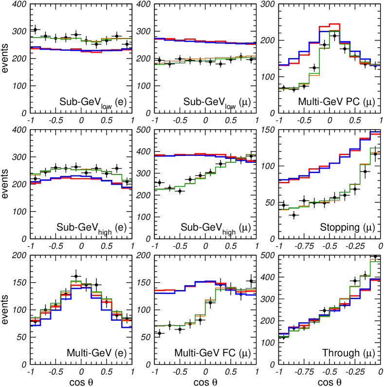
Figure 57: Comparison of our calculations with Super-Kamiokande ones. The blue and green lines show our predictions for no-oscillations and for $\Delta m^{2}=2.5\times 10^{-3}~{}\text{eV}^{2}$ and $\theta=45^{\circ}$, respectively. The red and orange lines are the corresponding calculations of the Super-Kamiokande collaborations. Black crosses show the experimental results with their statistical errors.

In order to verify the quality of the simulation, in Fig. 57 we compare the simulated predictions of the event number for the different SK data samples with those of the Super-Kamiokande collaboration, taken from Ref. [79]. The blue line gives the expected number of events for no oscillations, and should be compared with the red line. As can be seen, the simulation used in this review agrees quite well with those of the SK collaboration for all the data samples, with the exception of some small deformations in multi-GeV $e$-like events and in partially-contained events. In order to compensate for these discrepancies, we rescale our Monte-Carlo for no-oscillations so to match exactly the Super-Kamiokande prediction. After this correction, we turn to the oscillation case and we plot the expected number of events for $\Delta m^{2}=2.5\times 10^{-3}~{}\text{eV}^{2}$ and $\theta=45^{\circ}$ (green line). This line is in excellent agreement with the Super-Kamiokande expectations (orange line), which we take from Ref. [79].

A.2 Details of the $\chi^{2}$ calculation

The basic idea of the pull method consists in parametrizing the systematic errors and the theoretical uncertainties in terms of a set of variables $\{\xi_{i}\}$, called pulls, which are then treated on the same footing as the other parameters of the model. The $\chi^{2}$ function can be decomposed into the sum of two parts:

$$\chi^{2}(\vec{\omega},\vec{\xi})=\chi^{2}_{\text{data}}(\vec{\omega},\vec{\xi})+\chi^{2}_{\text{pulls}}(\vec{\xi}),$$ (359)

where $\vec{\omega}$ denotes the parameters of the model, $\chi^{2}_{\text{data}}$ is the usual term describing the deviation of the experimental results from their theoretical predictions, and the extra term $\chi^{2}_{\text{pulls}}$ provides proper penalties to account for deviations of the systematics and the theoretical inputs from their nominal value.

For the Super-Kamiokande experiment $\chi^{2}_{\text{pulls}}(\vec{\xi})$ can be properly written as a positive quadratic function of $\xi_{i}$. It is convenient to define the pulls in such a way that for each source of systematics or theoretical input $i$ the value $\xi_{i}=0$ corresponds to the “expected value” reported by the collaboration or predicted by the theory, and $\xi_{i}=\pm 1$ corresponds to a $1\sigma$ deviation. Since pulls describing different systematics and theoretical inputs are assumed to be uncorrelated, the expression of $\chi^{2}_{\text{pulls}}$ is very simple:

$$\chi^{2}_{\text{pulls}}(\vec{\xi})=\sum_{i,\text{theory}}\xi_{i}^{2}+\sum_{i,\text{syst}}\xi_{i}^{2}.$$ (360)

The form of $\chi^{2}_{\text{data}}$ depends on the expected distribution of the experimental results. The outcome of the Super-Kamiokande experiment is the number of events observed in each energy and zenith-angle bin, which follows a Poisson distribution. However, since the number of events in each bin is large, $\chi^{2}_{\text{data}}$ can be well approximated by a quadratic function of the differences between observed and expected rates of events:

$$\chi^{2}_{\text{data}}(\vec{\omega},\vec{\xi})=\sum_{n}\left(\frac{R_{n}^{\text{th}}(\vec{\omega},\vec{\xi})-R_{n}^{\text{ex}}}{\sigma_{n}^{\text{stat}}}\right)^{2}$$ (361)

where $R_{n}^{\text{th}}$ ($R_{n}^{\text{ex}}$) is the ratio between the expected (observed) number of events and the theoretical Monte Carlo for the case of no oscillations. Note that the dependence of $\chi^{2}_{\text{data}}$ on both the parameters $\vec{\omega}$ and the pulls $\vec{\xi}$ is entirely through $R_{n}^{\text{th}}(\vec{\omega},\vec{\xi})$. In the pull approach, $\vec{\omega}$ and $\vec{\xi}$ play a very similar role, and in principle should be treated in the same way. However, for the Super-Kamiokande experiment the bounds on $\vec{\xi}$ implied by $\chi^{2}_{\text{pulls}}$ are in general significantly stronger than those implied by $\chi^{2}_{\text{data}}$, and is therefore a good approximation to retain the dependence $\chi^{2}_{\text{data}}$ on $\vec{\xi}$ only to the lowest orders. This is done by expanding $R_{n}^{\text{th}}(\vec{\omega},\vec{\xi})$ in powers of $\xi_{i}$ up to the first order:

$$R_{n}^{\text{th}}(\vec{\omega},\vec{\xi})\approx R_{n}^{\text{th}}(\vec{\omega})\left[1+\sum_{i}\pi_{n}^{i}(\vec{\omega})\,\xi_{i}\right],\quad\text{where}\quad\left\{\begin{aligned} R_{n}^{\text{th}}(\vec{\omega})&\equiv R_{n}^{\text{th}}(\vec{\omega},0),\\[2.84526pt] R_{n}^{\text{th}}(\vec{\omega})\,\pi_{n}^{i}(\vec{\omega})&\equiv\left.\frac{\partial R_{n}^{\text{th}}(\vec{\omega},\vec{\xi})}{\partial\xi_{i}}\right|_{\vec{\xi}=0}.\end{aligned}\right.$$ (362)

It is easy to prove [158] that under the approximation (362) the pull definition given in (359) is mathematically equivalent to the usual covariance definition of the $\chi^{2}$.

In the present work, we have neglected the dependence of $\pi_{n}^{i}$ on the neutrino parameters $\vec{\omega}$. With this approximation, we can write:

$$\chi^{2}(\vec{\omega})=\min_{\vec{\xi}}\left[\sum_{n}\left(\frac{R_{n}^{\text{th}}(\vec{\omega})\left[1+\sum_{i}\pi_{n}^{i}\,\xi_{i}\right]-R_{n}^{\text{ex}}}{\sigma_{n}^{\text{stat}}}\right)^{2}+\sum_{i,\text{theory}}\xi_{i}^{2}+\sum_{i,\text{syst}}\xi_{i}^{2}\right]$$ (363)

where we have introduced the function $\chi^{2}(\vec{\omega})=\min_{\{\xi_{i}\}}\chi^{2}(\vec{\omega},\vec{\xi})$. It is clear from Eq. (363) that in the present approach the systematic and theoretical uncertainties are completely characterized by the set of quantities $\{\pi_{n}^{i}\}$, which describe the strength of the “coupling” between the pull $\xi_{i}$ and the observable $R^{\text{th}}_{n}$. In the rest of this section we will discuss in detail how we have parametrized and taken into account the various sources of uncertainty.

A.2.1 Theoretical uncertainties

Sample		$\pi^{\text{flux}}_{\text{tilt}}$	$\pi^{\text{flux}}_{\text{zenith}}$	$\pi^{\text{flux}}_{\text{anti}}$	$\pi^{\text{flux}}_{\text{ratio}}$	$\pi^{\text{cross}}_{\text{QE}}$	$\pi^{\text{cross}}_{\text{$1\pi$}}$	$\pi^{\text{cross}}_{\text{DIS}}$
	01	$-1.68$	$-0.16$	$+0.63$	$-1.00$	$+0.81$	$+0.10$	$+0.09$
	02	$-1.68$	$-0.14$	$+0.63$	$-1.00$	$+0.81$	$+0.10$	$+0.09$
	03	$-1.68$	$-0.11$	$+0.62$	$-1.00$	$+0.81$	$+0.11$	$+0.09$
	04	$-1.68$	$-0.09$	$+0.62$	$-1.00$	$+0.81$	$+0.11$	$+0.09$
$\text{sub-GeV}_{\text{low}}$ $e$	05	$-1.68$	$-0.06$	$+0.63$	$-1.00$	$+0.80$	$+0.11$	$+0.09$
	06	$-1.68$	$-0.04$	$+0.63$	$-1.00$	$+0.81$	$+0.11$	$+0.09$
	07	$-1.68$	$-0.01$	$+0.63$	$-1.00$	$+0.81$	$+0.10$	$+0.09$
	08	$-1.68$	$+0.02$	$+0.64$	$-1.00$	$+0.81$	$+0.10$	$+0.09$
	09	$-1.69$	$+0.04$	$+0.64$	$-1.00$	$+0.82$	$+0.09$	$+0.09$
	10	$-1.69$	$+0.07$	$+0.65$	$-1.00$	$+0.83$	$+0.09$	$+0.09$
	01	$-0.75$	$-0.64$	$+0.52$	$-1.00$	$+0.61$	$+0.28$	$+0.11$
	02	$-0.74$	$-0.49$	$+0.51$	$-1.00$	$+0.60$	$+0.28$	$+0.12$
	03	$-0.74$	$-0.35$	$+0.51$	$-1.00$	$+0.59$	$+0.29$	$+0.12$
	04	$-0.73$	$-0.21$	$+0.50$	$-1.00$	$+0.58$	$+0.29$	$+0.13$
$\text{sub-GeV}_{\text{high}}$ $e$	05	$-0.73$	$-0.08$	$+0.50$	$-1.00$	$+0.57$	$+0.30$	$+0.13$
	06	$-0.72$	$+0.05$	$+0.50$	$-1.00$	$+0.57$	$+0.30$	$+0.13$
	07	$-0.72$	$+0.19$	$+0.50$	$-1.00$	$+0.58$	$+0.29$	$+0.13$
	08	$-0.73$	$+0.32$	$+0.50$	$-1.00$	$+0.59$	$+0.29$	$+0.13$
	09	$-0.73$	$+0.47$	$+0.51$	$-1.00$	$+0.60$	$+0.28$	$+0.12$
	10	$-0.74$	$+0.63$	$+0.52$	$-1.00$	$+0.61$	$+0.28$	$+0.12$
	01	$+0.29$	$-0.84$	$+0.27$	$-1.00$	$+0.49$	$+0.23$	$+0.28$
	02	$+0.32$	$-0.64$	$+0.27$	$-1.00$	$+0.48$	$+0.22$	$+0.29$
	03	$+0.35$	$-0.44$	$+0.26$	$-1.00$	$+0.47$	$+0.22$	$+0.31$
	04	$+0.41$	$-0.25$	$+0.26$	$-1.00$	$+0.45$	$+0.21$	$+0.33$
multi-GeV $e$	05	$+0.48$	$-0.08$	$+0.25$	$-1.00$	$+0.44$	$+0.21$	$+0.35$
	06	$+0.48$	$+0.08$	$+0.25$	$-1.00$	$+0.43$	$+0.21$	$+0.36$
	07	$+0.41$	$+0.25$	$+0.26$	$-1.00$	$+0.45$	$+0.21$	$+0.33$
	08	$+0.36$	$+0.44$	$+0.26$	$-1.00$	$+0.47$	$+0.22$	$+0.31$
	09	$+0.33$	$+0.63$	$+0.27$	$-1.00$	$+0.48$	$+0.22$	$+0.30$
	10	$+0.30$	$+0.84$	$+0.27$	$-1.00$	$+0.49$	$+0.23$	$+0.29$

Table 7: Coupling factors of the flux and cross-section pulls with fully-contained $e$-like events.

Sample		$\pi^{\text{flux}}_{\text{tilt}}$	$\pi^{\text{flux}}_{\text{zenith}}$	$\pi^{\text{flux}}_{\text{anti}}$	$\pi^{\text{flux}}_{\text{ratio}}$	$\pi^{\text{cross}}_{\text{QE}}$	$\pi^{\text{cross}}_{\text{$1\pi$}}$	$\pi^{\text{cross}}_{\text{DIS}}$
	01	$-1.38$	$-0.19$	$+0.64$	$+1.00$	$+0.78$	$+0.14$	$+0.08$
	02	$-1.38$	$-0.12$	$+0.64$	$+1.00$	$+0.77$	$+0.14$	$+0.08$
	03	$-1.38$	$-0.05$	$+0.63$	$+1.00$	$+0.77$	$+0.14$	$+0.09$
	04	$-1.38$	$+0.01$	$+0.63$	$+1.00$	$+0.77$	$+0.15$	$+0.09$
$\text{sub-GeV}_{\text{low}}$ $\mu$	05	$-1.38$	$+0.08$	$+0.62$	$+1.00$	$+0.76$	$+0.15$	$+0.09$
	06	$-1.38$	$+0.14$	$+0.62$	$+1.00$	$+0.75$	$+0.16$	$+0.09$
	07	$-1.37$	$+0.20$	$+0.61$	$+1.00$	$+0.74$	$+0.16$	$+0.10$
	08	$-1.37$	$+0.26$	$+0.60$	$+1.00$	$+0.73$	$+0.17$	$+0.10$
	09	$-1.37$	$+0.31$	$+0.60$	$+1.00$	$+0.72$	$+0.18$	$+0.10$
	10	$-1.37$	$+0.37$	$+0.59$	$+1.00$	$+0.71$	$+0.19$	$+0.10$
	01	$-0.71$	$-0.66$	$+0.46$	$+1.00$	$+0.60$	$+0.27$	$+0.12$
	02	$-0.70$	$-0.49$	$+0.46$	$+1.00$	$+0.60$	$+0.28$	$+0.13$
	03	$-0.70$	$-0.32$	$+0.46$	$+1.00$	$+0.60$	$+0.27$	$+0.13$
	04	$-0.69$	$-0.14$	$+0.46$	$+1.00$	$+0.60$	$+0.27$	$+0.14$
$\text{sub-GeV}_{\text{high}}$ $\mu$	05	$-0.68$	$+0.02$	$+0.46$	$+1.00$	$+0.59$	$+0.26$	$+0.14$
	06	$-0.68$	$+0.18$	$+0.44$	$+1.00$	$+0.58$	$+0.27$	$+0.14$
	07	$-0.68$	$+0.32$	$+0.44$	$+1.00$	$+0.57$	$+0.29$	$+0.14$
	08	$-0.68$	$+0.45$	$+0.43$	$+1.00$	$+0.56$	$+0.29$	$+0.14$
	09	$-0.69$	$+0.57$	$+0.44$	$+1.00$	$+0.57$	$+0.29$	$+0.14$
	10	$-0.69$	$+0.70$	$+0.45$	$+1.00$	$+0.58$	$+0.28$	$+0.14$
	01	$+0.23$	$-0.85$	$+0.24$	$+1.00$	$+0.51$	$+0.22$	$+0.27$
	02	$+0.22$	$-0.65$	$+0.23$	$+1.00$	$+0.50$	$+0.22$	$+0.27$
	03	$+0.22$	$-0.46$	$+0.22$	$+1.00$	$+0.50$	$+0.22$	$+0.27$
	04	$+0.22$	$-0.25$	$+0.22$	$+1.00$	$+0.49$	$+0.23$	$+0.28$
multi-GeV $\mu$	05	$+0.25$	$-0.03$	$+0.22$	$+1.00$	$+0.49$	$+0.21$	$+0.30$
	06	$+0.26$	$+0.15$	$+0.19$	$+1.00$	$+0.48$	$+0.22$	$+0.30$
	07	$+0.24$	$+0.31$	$+0.20$	$+1.00$	$+0.48$	$+0.23$	$+0.29$
	08	$+0.23$	$+0.47$	$+0.22$	$+1.00$	$+0.49$	$+0.22$	$+0.28$
	09	$+0.23$	$+0.65$	$+0.23$	$+1.00$	$+0.50$	$+0.22$	$+0.28$
	10	$+0.24$	$+0.85$	$+0.24$	$+1.00$	$+0.50$	$+0.22$	$+0.28$

Table 8: Coupling factors of the flux and cross-section pulls with fully-contained $\mu$-like events.

Sample		$\pi^{\text{flux}}_{\text{tilt}}$	$\pi^{\text{flux}}_{\text{zenith}}$	$\pi^{\text{flux}}_{\text{anti}}$	$\pi^{\text{flux}}_{\text{ratio}}$	$\pi^{\text{cross}}_{\text{QE}}$	$\pi^{\text{cross}}_{\text{$1\pi$}}$	$\pi^{\text{cross}}_{\text{DIS}}$
	01	$+1.42$	$-0.86$	$+0.29$	$+1.00$	$+0.22$	$+0.16$	$+0.63$
	02	$+1.46$	$-0.67$	$+0.28$	$+1.00$	$+0.21$	$+0.16$	$+0.63$
	03	$+1.56$	$-0.47$	$+0.28$	$+1.00$	$+0.21$	$+0.15$	$+0.64$
	04	$+1.73$	$-0.25$	$+0.28$	$+1.00$	$+0.17$	$+0.14$	$+0.69$
partially-contained $\mu$	05	$+1.78$	$-0.05$	$+0.25$	$+1.00$	$+0.16$	$+0.12$	$+0.72$
	06	$+1.66$	$+0.11$	$+0.23$	$+1.00$	$+0.18$	$+0.13$	$+0.70$
	07	$+1.52$	$+0.29$	$+0.25$	$+1.00$	$+0.19$	$+0.14$	$+0.67$
	08	$+1.44$	$+0.47$	$+0.27$	$+1.00$	$+0.21$	$+0.15$	$+0.64$
	09	$+1.41$	$+0.67$	$+0.28$	$+1.00$	$+0.21$	$+0.15$	$+0.64$
	10	$+1.40$	$+0.86$	$+0.30$	$+1.00$	$+0.21$	$+0.15$	$+0.63$
	01	$+1.88$	$-0.93$	$+0.32$	$+1.00$	$+0.16$	$+0.11$	$+0.72$
	02	$+1.87$	$-0.83$	$+0.32$	$+1.00$	$+0.17$	$+0.12$	$+0.72$
	03	$+1.88$	$-0.73$	$+0.31$	$+1.00$	$+0.17$	$+0.12$	$+0.72$
	04	$+1.90$	$-0.63$	$+0.31$	$+1.00$	$+0.17$	$+0.11$	$+0.72$
stopping $\mu$	05	$+1.96$	$-0.53$	$+0.31$	$+1.00$	$+0.17$	$+0.11$	$+0.72$
	06	$+2.03$	$-0.43$	$+0.31$	$+1.00$	$+0.16$	$+0.11$	$+0.73$
	07	$+2.12$	$-0.32$	$+0.32$	$+1.00$	$+0.14$	$+0.11$	$+0.75$
	08	$+2.17$	$-0.21$	$+0.31$	$+1.00$	$+0.12$	$+0.10$	$+0.78$
	09	$+2.15$	$-0.11$	$+0.29$	$+1.00$	$+0.12$	$+0.09$	$+0.79$
	10	$+2.11$	$-0.02$	$+0.26$	$+1.00$	$+0.13$	$+0.09$	$+0.79$
	01	$+4.53$	$-0.95$	$+0.32$	$+1.00$	$+0.03$	$+0.01$	$+0.96$
	02	$+4.47$	$-0.85$	$+0.32$	$+1.00$	$+0.03$	$+0.01$	$+0.96$
	03	$+4.46$	$-0.75$	$+0.32$	$+1.00$	$+0.03$	$+0.01$	$+0.96$
	04	$+4.46$	$-0.65$	$+0.32$	$+1.00$	$+0.03$	$+0.01$	$+0.96$
through-going $\mu$	05	$+4.47$	$-0.55$	$+0.31$	$+1.00$	$+0.03$	$+0.01$	$+0.97$
	06	$+4.46$	$-0.45$	$+0.31$	$+1.00$	$+0.02$	$+0.01$	$+0.97$
	07	$+4.44$	$-0.34$	$+0.30$	$+1.00$	$+0.02$	$+0.01$	$+0.97$
	08	$+4.42$	$-0.24$	$+0.29$	$+1.00$	$+0.02$	$+0.01$	$+0.97$
	09	$+4.41$	$-0.14$	$+0.28$	$+1.00$	$+0.03$	$+0.01$	$+0.96$
	10	$+4.44$	$-0.05$	$+0.26$	$+1.00$	$+0.03$	$+0.01$	$+0.96$

Table 9: Coupling factors of the flux and cross-section pulls with partially-contained and upgoing $\mu$-like events.

Theoretical uncertainties arise from our limited knowledge of the atmospheric neutrino fluxes and cross-sections. The corresponding coefficients $\pi_{n}^{i}$ have been calculated assuming two-neutrino oscillations with $\Delta m^{2}=2.5\times 10^{-3}~{}\text{eV}^{2}$ and $\theta=45^{\circ}$, and are listed in Tables 7, 8 and 9.

We have parametrized flux uncertainties in terms of six pulls: $\xi^{\text{flux}}_{\text{norm}}$, $\xi^{\text{flux}}_{\text{tilt}}$, $\xi^{\text{flux}}_{\text{zenith}}$, $\xi^{\text{flux}}_{\text{anti}}$, $\xi^{\text{flux}}_{\text{ratio}}$ and $\xi^{\text{flux}}_{\text{multi}}$.

• $\xi^{\text{flux}}_{\text{norm}}$ (20%) is a total normalization error, with the same coupling $\pi^{\text{flux}}_{\text{norm}}=1$ to all the data samples;

• $\xi^{\text{flux}}_{\text{tilt}}$ (5%) is a“tilt” factor which parametrizes possible deformations of the flux energy spectrum:

  $$\Phi_{\delta}(E)=\Phi_{0}(E)\left(\frac{E}{E_{0}}\right)^{\delta}\approx\Phi_{0}(E)\left[1+\delta\ln\frac{E}{E_{0}}\right]\,.$$ (364)

  The uncertainty on the factor $\delta$ is 5%, and in analogy with Ref. [419] we have chosen $E_{0}=2$ GeV;

• $\xi^{\text{flux}}_{\text{zenith}}$ (5%) describes the uncertainty associated to the up-down asymmetry;

• $\xi^{\text{flux}}_{\text{anti}}$ (5%) describes the uncertainty associated to the $\nu/\bar{\nu}$ asymmetry;

• $\xi^{\text{flux}}_{\text{ratio}}$ (2.5%) parametrizes the uncertainty on the $\nu_{\mu}/\nu_{e}$ ratio.

• $\xi^{\text{flux}}_{\text{multi}}$ (5%) is an extra normalization factor which affects only fully-contained multi-GeV events (both $e$-like and $\mu$-like). Its corresponding coupling $\pi^{\text{flux}}_{\text{multi}}$ is $1$ for FC multi-GeV events and $0$ for all the other samples.

Concerning cross-section uncertainties, we properly take into account the contributions to the total number of observed events coming from three different types of charged-current interactions: quasi-elastic neutrino scattering (QE), 1-pion production ($1\pi$), and deep-inelastic scattering (DIS). We neglect for simplicity coherent scattering on oxygen and neutral-current interactions, which contribute only marginally to the considered data samples. For each different type of neutrino interactions we introduce two pulls:

• $\xi^{\text{QE}}_{\text{norm}}$, $\xi^{1\pi}_{\text{norm}}$, $\xi^{\text{DIS}}_{\text{norm}}$ (15%) describe the total normalization errors;

• $\xi^{\text{QE}}_{\text{ratio}}$, $\xi^{1\pi}_{\text{ratio}}$, $\xi^{\text{DIS}}_{\text{ratio}}$ ($-0.5\%$ for electrons and $+0.5\%$ for muons) parametrize the uncertainty of the $\sigma^{i}_{\nu_{\mu}}/\sigma^{i}_{\nu_{e}}$ ratios.

The fraction of events for each data sample originating from the different types of neutrino interactions is based on our own calculations, however we have verified that it is consistent with the numbers listed in Table 8.2 of Ref. [419] (after neglecting event misidentification and neutral-current contributions and rescaling the factors so that the sum is 100%).

A.2.2 Systematic uncertainties

Sample	$[\pi\xi]^{\text{sys}}_{\text{hadron}}$	$[\pi\xi]^{\text{sys}}_{\text{$\mu/e$}}$	$[\pi\xi]^{\text{sys}}_{\text{ring}}$	$[\pi\xi]^{\text{sys}}_{\text{f-vol}}$	$[\pi\xi]^{\text{sys}}_{\text{E-cal}}$
sub-GeV $e$	$-0.25\%$	$-1.1\%$	$-0.75\%$	$-0.3\%$	$-0.4\%$
mid-GeV $e$	$-0.25\%$	$-1.1\%$	$-0.75\%$	$-0.3\%$	$-0.4\%$
multi-GeV $e$	$-0.50\%$	$-1.6\%$	$-2.75\%$	$-0.5\%$	$+0.3\%$
sub-GeV $\mu$	$+0.25\%$	$+1.1\%$	$+0.75\%$	$+0.3\%$	$+0.4\%$
mid-GeV $\mu$	$+0.25\%$	$+1.1\%$	$+0.75\%$	$+0.3\%$	$+0.4\%$
multi-GeV $\mu$	$+0.50\%$	$+1.6\%$	$+2.75\%$	$+0.5\%$	$-0.3\%$
part-cont $\mu$	$-0.50\%$	$+1.6\%$	$-1.25\%$	$+0.5\%$	$-3.3\%$
stopping $\mu$	—	—	$-0.30\%$	$+0.7\%$	$-0.3\%$
through $\mu$	—	—	$-0.30\%$	$+0.7\%$	$-0.3\%$

Sample	$[\pi\xi]^{\text{sys}}_{\text{PC-nrm}}$	$[\pi\xi]^{\text{sys}}_{\text{track}}$	$[\pi\xi]^{\text{sys}}_{\text{up-eff}}$	$[\pi\xi]^{\text{sys}}_{\text{t-sep}}$
part-cont $\mu$	$5.27\%$	—	—	—
stopping $\mu$	—	$6.4\%$	$1.0\%$	$1.0\%$
through $\mu$	—	$1.4\%$	$1.0\%$	—

Table 10: Coupling factors of the systematics pulls $[\pi\xi]^{\text{sys}}_{\text{hadron}}$, $[\pi\xi]^{\text{sys}}_{\text{$\mu/e$}}$, $[\pi\xi]^{\text{sys}}_{\text{ring}}$, $[\pi\xi]^{\text{sys}}_{\text{f-vol}}$, $[\pi\xi]^{\text{sys}}_{\text{E-cal}}$, $[\pi\xi]^{\text{sys}}_{\text{PC-nrm}}$, $[\pi\xi]^{\text{sys}}_{\text{FC/PC}}$, $[\pi\xi]^{\text{sys}}_{\text{track}}$, $[\pi\xi]^{\text{sys}}_{\text{up-eff}}$ and $[\pi\xi]^{\text{sys}}_{\text{t-sep}}$ with the various observables. The coefficients are the same for all the bins in a given data sample.

The systematics uncertainties of the Super-Kamiokande experiment are derived from Tables 9.2, 9.3, 9.4 and 9.5 of Ref. [419]. In Table 10 we list the product of the given uncertainty $\xi_{i}$ with the corresponding coupling $\pi_{n}^{i}$. We include in our calculations the following sources of systematics:

• $\xi^{\text{sys}}_{\text{hadron}}$ is the uncertainty associated with the simulation of hadronic interactions;

• $\xi^{\text{sys}}_{\mu/e}$ describes the errors in the particle identification procedure;

• $\xi^{\text{sys}}_{\text{ring}}$ is the uncertainty coming from the ring-counting procedure;

• $\xi^{\text{sys}}_{\text{f-vol}}$ is the uncertainty in the fiducial volume determination, introduced by the vertex fitter procedure;

• $\xi^{\text{sys}}_{\text{E-cal}}$ is the uncertainty in the energy calibration;

• $\xi^{\text{sys}}_{\text{PC-nrm}}$ accounts for all the errors which are unique to partially-contained events;

• $\xi^{\text{sys}}_{\text{track}}$ is the uncertainty in the track reconstruction of upgoing muons;

• $\xi^{\text{sys}}_{\text{up-eff}}$ is the detection efficiency of upgoing muons;

• $\xi^{\text{sys}}_{\text{t-sep}}$ is the uncertainty in the separation of stopping and through-going events.

References

- [1] F. Reines and C. L. Cowan, Phys. Rev. 113 (1959) 273.
- [2] W. Pauli, letter sent to the Tubingen conference, Dec. 1930.
- [3] M. C. Gonzalez-Garcia and Y. Nir, Rev. Mod. Phys. 75 (2003) 345 [arXiv:hep-ph/0202058].
- [4] B. Pontecorvo, Sov. Phys. JETP 26 (1968) 984 [Zh. Eksp. Teor. Fiz. 53 (1967) 1717].
- [5] V. N. Gribov and B. Pontecorvo, Phys. Lett. B 28 (1969) 493.
- [6] S. M. Bilenky, C. Giunti and W. Grimus, Prog. Part. Nucl. Phys. 43 (1999) 1 [arXiv:hep-ph/9812360].
- [7] A. D. Dolgov, Phys. Rept. 370 (2002) 333 [arXiv:hep-ph/0202122].
- [8] V. Barger, D. Marfatia and K. Whisnant, Int. J. Mod. Phys. E 12 (2003) 569 [arXiv:hep-ph/0308123].
- [9] S. Pakvasa and J. W. F. Valle, Proc. Indian Natl. Sci. Acad. 70A (2004) 189 [arXiv:hep-ph/0301061].
- [10] M. Maltoni, T. Schwetz, M. A. Tortola and J. W. F. Valle, New J. Phys. 6 (2004) 122 [arXiv:hep-ph/0405172].
- [11] G. L. Fogli, E. Lisi, A. Marrone and A. Palazzo, Prog. Part. Nucl. Phys. 57 (2006) 742 [arXiv:hep-ph/0506083].
- [12] R. N. Mohapatra and A. Y. Smirnov, Ann. Rev. Nucl. Part. Sci. 56 (2006) 569 [arXiv:hep-ph/0603118].
- [13] J. Lesgourgues and S. Pastor, Phys. Rept. 429 (2006) 307 [arXiv:astro-ph/0603494].
- [14] A. Strumia and F. Vissani, arXiv:hep-ph/0606054.
- [15] H. Nunokawa, S. J. Parke and J. W. F. Valle, arXiv:0710.0554 [hep-ph].
- [16] J. N. Bahcall, Neutrino Astrophysics, Cambridge University Press (1989).
- [17] F. Boehm and P. Vogel, Physics of Massive Neutrinos, Cambridge University Press (1987).
- [18] B. Kayser, F. Gibrat-Debu and F. Perrier, World Sci. Lect. Notes Phys. 25 (1989) 1.
- [19] T. K. Gaisser, Cosmic Rays And Particle Physics, Cambridge University Press (1990).
- [20] C. W. Kim and A. Pevsner, Contemp. Concepts Phys. 8 (1993) 1.
- [21] R. N. Mohapatra and P. B. Pal, World Sci. Lect. Notes Phys. 60 (1998) 1 [World Sci. Lect. Notes Phys. 72 (2004) 1].
- [22] M. Fukugita and T. Yanagida, Physics of neutrinos and applications to astrophysics, Springer, Berlin, Germany (2003).
- [23] W. M. Yao et al. [Particle Data Group], J. Phys. G 33 (2006) 1.
- [24] P. Minkowski, Phys. Lett. B 67 (1977) 421.
- [25] P. Ramond, Invited talk given at Sanibel Symposium, Palm Coast, Fla., Feb 25 – Mar 2, 1979, published in Paris 2004, Seesaw 25 265–280 [arXiv:hep-ph/9809459].
- [26] M. Gell-Mann, P. Ramond and R. Slansky, in Supergravity, edited by P. van Nieuwenhuizen and D. Z. Freedman (North Holland).
- [27] T. Yanagida, In Proceedings of the Workshop on the Baryon Number of the Universe and Unified Theories, Tsukuba, Japan, 13–14 Feb 1979, edited by O. Sawada and A. Sugamoto (KEK).
- [28] R. N. Mohapatra and G. Senjanovic, Phys. Rev. Lett. 44 (1980) 912.
- [29] Z. Maki, M. Nakagawa and S. Sakata, Prog. Theor. Phys. 28 (1962) 870.
- [30] J. Schechter and J. W. F. Valle, Phys. Rev. D 21 (1980) 309.
- [31] J. Schechter and J. W. F. Valle, Phys. Rev. D 22 (1980) 2227.
- [32] J. Schechter and J. W. F. Valle, Phys. Rev. D 24 (1981) 1883 [Erratum-ibid. D 25 (1982) 283].
- [33] M. Kobayashi and T. Maskawa, Prog. Theor. Phys. 49 (1973) 652.
- [34] L. Wolfenstein, Phys. Rev. D 17 (1978) 2369.
- [35] A. Halprin, Phys. Rev. D 34 (1986) 3462.
- [36] P. D. Mannheim, Phys. Rev. D 37 (1988) 1935.
- [37] A. J. Baltz and J. Weneser, Phys. Rev. D 37 (1988) 3364.
- [38] L. Landau, Phys. Z. Sov. 2 (1932) 46.
- [39] C. Zener, Proc. Roy. Soc. Lond. A 137 (1932) 696.
- [40] T. K. Kuo and J. T. Pantaleone, Rev. Mod. Phys. 61 (1989) 937.
- [41] S. J. Parke, Phys. Rev. Lett. 57 (1986) 1275.
- [42] W. C. Haxton, Phys. Rev. Lett. 57 (1986) 1271.
- [43] S. T. Petcov, Phys. Lett. B 191 (1987) 299.
- [44] S. P. Mikheev and A. Y. Smirnov, Sov. J. Nucl. Phys. 42 (1985) 913 [Yad. Fiz. 42 (1985) 1441].
- [45] J. N. Bahcall, A. M. Serenelli and S. Basu, Astrophys. J. 621 (2005) L85 [arXiv:astro-ph/0412440].
- [46] R. J. Davis, D. S. Harmer and K. C. Hoffman, Phys. Rev. Lett. 20 (1968) 1205.
- [47] B. T. Cleveland et al., Astrophys. J. 496 (1998) 505.
- [48] J. N. Abdurashitov et al. [SAGE Collaboration], J. Exp. Theor. Phys. 95 (2002) 181 [Zh. Eksp. Teor. Fiz. 122 (2002) 211] [arXiv:astro-ph/0204245].
- [49] W. Hampel et al. [GALLEX Collaboration], Phys. Lett. B 447 (1999) 127.
- [50] M. Altmann et al. [GNO Collaboration], Phys. Lett. B 616 (2005) 174 [arXiv:hep-ex/0504037].
- [51] Y. Fukuda et al. [Kamiokande Collaboration], Phys. Rev. Lett. 77 (1996) 1683.
- [52] M. B. Smy et al. [Super-Kamiokande Collaboration], Phys. Rev. D 69 (2004) 011104 [arXiv:hep-ex/0309011].
- [53] Q. R. Ahmad et al. [SNO Collaboration], Phys. Rev. Lett. 87 (2001) 071301 [arXiv:nucl-ex/0106015].
- [54] Q. R. Ahmad et al. [SNO Collaboration], Phys. Rev. Lett. 89, 011301 (2002) [arXiv:nucl-ex/0204008].
- [55] Q. R. Ahmad et al. [SNO Collaboration], Phys. Rev. Lett. 89, 011302 (2002) [arXiv:nucl-ex/0204009].
- [56] S. N. Ahmed et al. [SNO Collaboration], Phys. Rev. Lett. 92 (2004) 181301 [arXiv:nucl-ex/0309004].
- [57] B. Aharmim et al. [SNO Collaboration], Phys. Rev. C 72 (2005) 055502 [arXiv:nucl-ex/0502021].
- [58] L. Oberauer, Nucl. Phys. Proc. Suppl. 77 (1999) 48.
- [59] Borexino Collaboration, arXiv:0708.2251 [astro-ph].
- [60] J. N. Bahcall, N. A. Bahcall and G. Shaviv, Phys. Rev. Lett. 20 (1968) 1209.
- [61] J. N. Bahcall and R. Davis, Science 191 (1976) 264.
- [62] F. Reines et al., Phys. Rev. Lett. 15 (1965) 429.
- [63] C. V. Achar et al., Phys. Lett. 18 (1965) 196.
- [64] See the talk by C. Walter at The XXXIII International Conference on High Energy Physics, Moscow, Russian Federation, July 26 – August 2, 2006.
- [65] G. D. Barr, T. K. Gaisser, P. Lipari, S. Robbins and T. Stanev, Phys. Rev. D 70 (2004) 023006 [arXiv:astro-ph/0403630].
- [66] M. Honda, T. Kajita, K. Kasahara and S. Midorikawa, Phys. Rev. D 70 (2004) 043008 [arXiv:astro-ph/0404457].
- [67] G. Battistoni, A. Ferrari, T. Montaruli and P. R. Sala, Astropart. Phys. 19 (2003) 269 [Erratum-ibid. 19 (2003) 291] [arXiv:hep-ph/0207035].
- [68] Y. Liu, L. Derome and M. Buenerd, Phys. Rev. D 67 (2003) 073022 [arXiv:astro-ph/0211632].
- [69] J. Wentz, I. M. Brancus, A. Bercuci, D. Heck, J. Oehlschlager, H. Rebel and B. Vulpescu, Phys. Rev. D 67 (2003) 073020 [arXiv:hep-ph/0301199].
- [70] K. Daum et al. [Frejus Collaboration.], Z. Phys. C 66 (1995) 417.
- [71] M. Aglietta et al. [NUSEX Collaboration], Europhys. Lett. 8 (1989) 611.
- [72] R. Becker-Szendy et al., Phys. Rev. D 46 (1992) 3720.
- [73] Y. Fukuda et al. [Kamiokande Collaboration], Phys. Lett. B 335 (1994) 237.
- [74] Y. Fukuda et al. [Super-Kamiokande Collaboration], Phys. Rev. Lett. 81 (1998) 1562 [arXiv:hep-ex/9807003].
- [75] M. C. Sanchez et al. [Soudan 2 Collaboration], Phys. Rev. D 68 (2003) 113004 [arXiv:hep-ex/0307069].
- [76] M. Ambrosio et al. [MACRO Collaboration], Phys. Lett. B 517 (2001) 59 [arXiv:hep-ex/0106049].
- [77] Y. Ashie et al. [Super-Kamiokande Collaboration], Phys. Rev. D 71 (2005) 112005 [arXiv:hep-ex/0501064].
- [78] J. Hosaka et al. [Super-Kamiokande Collaboration], Phys. Rev. D 74 (2006) 032002 [arXiv:hep-ex/0604011].
- [79] See the talk by P.J. Litchfield at The XXII International Conference on Neutrino Physics, Santa Fe, New Mexico, June 13–19, 2006.
- [80] G. Zacek et al. [CALTECH-SIN-TUM Collaboration], Phys. Rev. D 34 (1986) 2621.
- [81] G. S. Vidyakin et al., JETP Lett. 59 (1994) 390 [Pisma Zh. Eksp. Teor. Fiz. 59 (1994) 364].
- [82] Y. Declais et al., Nucl. Phys. B 434 (1995) 503.
- [83] M. Apollonio et al. [CHOOZ Collaboration], Phys. Lett. B 466 (1999) 415 [arXiv:hep-ex/9907037].
- [84] A. Piepke [Palo Verde Collaboration], Prog. Part. Nucl. Phys. 48 (2002) 113.
- [85] A. Piepke [KamLAND Collaboration], Nucl. Phys. Proc. Suppl. 91 (2001) 99.
- [86] I. Shimizu [KamLAND Collaboration], talk given at the TAUP 2007 conference, Sendai, Japan, September 2007.
- [87] K. Eguchi et al. [KamLAND Collaboration], Phys. Rev. Lett. 90 (2003) 021802 [arXiv:hep-ex/0212021].
- [88] T. Araki et al. [KamLAND Collaboration], Phys. Rev. Lett. 94 (2005) 081801 [arXiv:hep-ex/0406035].
- [89] K. Nishikawa, Nucl. Phys. Proc. Suppl. 59 (1997) 289.
- [90] E. Ables et al. [MINOS Collaboration], FERMILAB-PROPOSAL-P-875 (1995).
- [91] S. H. Ahn et al. [K2K Collaboration], Phys. Lett. B 511 (2001) 178 [arXiv:hep-ex/0103001].
- [92] E. Aliu et al. [K2K Collaboration], Phys. Rev. Lett. 94 (2005) 081802 [arXiv:hep-ex/0411038].
- [93] D. G. Michael et al. [MINOS Collaboration], Phys. Rev. Lett. 97 (2006) 191801 [arXiv:hep-ex/0607088].
- [94] A. Weber [MINOS Collaboration], talk given at the EPS conference, Manchester, United Kingdom, July 2007.
- [95] M. Guler et al. [OPERA Collaboration], CERN-SPSC-2000-028, CERN-SPSC-P-318, LNGS-P25-00.
- [96] A. G. Cocco [OPERA Collaboration], Nucl. Phys. Proc. Suppl. 85 (2000) 125.
- [97] R. Acquafredda et al. [OPERA Collaboration], New J. Phys. 8 (2006) 303 [arXiv:hep-ex/0611023].
- [98] F. Dydak et al. [CDHS Collaboration], Phys. Lett. B 134 (1984) 281.
- [99] L. Borodovsky et al. [E776 Collaboration], Phys. Rev. Lett. 68 (1992) 274.
- [100] L. A. Ahrens et al. [E734 Collaboration], Phys. Rev. D 36 (1987) 702.
- [101] B. Armbruster et al. [KARMEN Collaboration], Phys. Rev. D 65 (2002) 112001 [arXiv:hep-ex/0203021].
- [102] N. Ushida et al. [E531 Collaboration], Phys. Rev. Lett. 57 (1986) 2897.
- [103] A. Romosan et al. [CCFR/NuTeV Collaboration], Phys. Rev. Lett. 78 (1997) 2912 [arXiv:hep-ex/9611013].
- [104] S. Avvakumov et al., Phys. Rev. Lett. 89 (2002) 011804 [arXiv:hep-ex/0203018].
- [105] K. S. McFarland et al. [CCFR/NuTeV Collaboration], Phys. Rev. Lett. 75 (1995) 3993 [arXiv:hep-ex/9506007].
- [106] D. Naples et al. [CCFR/NuTeV Collaboration], Phys. Rev. D 59 (1999) 031101 [arXiv:hep-ex/9809023].
- [107] E. Eskut et al. [CHORUS Collaboration], Phys. Lett. B 497 (2001) 8.
- [108] P. Astier et al. [NOMAD Collaboration], Nucl. Phys. B 611 (2001) 3 [arXiv:hep-ex/0106102].
- [109] A. Aguilar et al. [LSND Collaboration], Phys. Rev. D 64 (2001) 112007 [arXiv:hep-ex/0104049].
- [110] A. A. Aguilar-Arevalo et al. [MiniBooNE Collaboration], Phys. Rev. Lett. 98 (2007) 231801 [arXiv:0704.1500 [hep-ex]].
- [111] E. D. Church, K. Eitel, G. B. Mills and M. Steidl, Phys. Rev. D 66 (2002) 013001 [arXiv:hep-ex/0203023].
- [112] A. Bazarko [MiniBooNE Collaboration], Nucl. Phys. Proc. Suppl. 91 (2001) 210 [arXiv:hep-ex/0009056].
- [113] J. N. Bahcall, M. C. Gonzalez-Garcia and C. Pena-Garay, JHEP 0108 (2001) 014 [arXiv:hep-ph/0106258].
- [114] P. Lipari and M. Lusignoli, Phys. Rev. D 58 (1998) 073005 [arXiv:hep-ph/9803440].
- [115] S. Fukuda et al. [Super-Kamiokande Collaboration], Phys. Rev. Lett. 85 (2000) 3999 [arXiv:hep-ex/0009001].
- [116] K. Abe et al. [Super-Kamiokande Collaboration], Phys. Rev. Lett. 97 (2006) 171801 [arXiv:hep-ex/0607059].
- [117] S. M. Bilenky, J. Hosek and S. T. Petcov, Phys. Lett. B 94 (1980) 495.
- [118] P. Langacker, S. T. Petcov, G. Steigman and S. Toshev, Nucl. Phys. B 282 (1987) 589.
- [119] S. M. Bilenky, D. Nicolo and S. T. Petcov, Phys. Lett. B 538 (2002) 77 [arXiv:hep-ph/0112216].
- [120] T. K. Kuo and J. T. Pantaleone, Phys. Rev. Lett. 57 (1986) 1805.
- [121] X. Shi and D. N. Schramm, Phys. Lett. B 283 (1992) 305.
- [122] S. T. Petcov, Phys. Lett. B 434 (1998) 321 [arXiv:hep-ph/9805262].
- [123] E. K. Akhmedov, Nucl. Phys. B 538 (1999) 25 [arXiv:hep-ph/9805272].
- [124] E. K. Akhmedov, A. Dighe, P. Lipari and A. Y. Smirnov, Nucl. Phys. B 542 (1999) 3 [arXiv:hep-ph/9808270].
- [125] M. Chizhov, M. Maris and S. T. Petcov, arXiv:hep-ph/9810501.
- [126] J. Bernabeu, S. Palomares-Ruiz, A. Perez and S. T. Petcov, Phys. Lett. B 531 (2002) 90 [arXiv:hep-ph/0110071].
- [127] J. Bernabeu, S. Palomares Ruiz and S. T. Petcov, Nucl. Phys. B 669 (2003) 255 [arXiv:hep-ph/0305152].
- [128] S. Palomares-Ruiz and S. T. Petcov, Nucl. Phys. B 712 (2005) 392 [arXiv:hep-ph/0406096].
- [129] S. Choubey and P. Roy, Phys. Rev. D 73 (2006) 013006 [arXiv:hep-ph/0509197].
- [130] E. K. Akhmedov, M. Maltoni and A. Y. Smirnov, arXiv:hep-ph/0612285.
- [131] C. W. Kim and U. W. Lee, Phys. Lett. B 444 (1998) 204 [arXiv:hep-ph/9809491].
- [132] O. Yasuda, arXiv:hep-ph/9602342.
- [133] O. Yasuda, arXiv:hep-ph/9706546.
- [134] T. Sakai and T. Teshima, Prog. Theor. Phys. 102 (1999) 629 [arXiv:hep-ph/9901219].
- [135] A. Strumia, JHEP 9904 (1999) 026 [arXiv:hep-ph/9904245].
- [136] G. L. Fogli, E. Lisi, A. Marrone and A. Palazzo, Proceedings of the 3rd Workshop on Neutrino Oscillations and Their Origin (NOON 2001), Kashiwa, Japan, 5–8 Dec 2001.
- [137] O. L. G. Peres and A. Y. Smirnov, Phys. Lett. B 456 (1999) 204 [arXiv:hep-ph/9902312].
- [138] M. C. Gonzalez-Garcia and M. Maltoni, Eur. Phys. J. C 26 (2003) 417 [arXiv:hep-ph/0202218].
- [139] M. C. Gonzalez-Garcia, M. Maltoni and A. Y. Smirnov, Phys. Rev. D 70 (2004) 093005 [arXiv:hep-ph/0408170].
- [140] O. L. G. Peres and A. Y. Smirnov, Nucl. Phys. Proc. Suppl. 110 (2002) 355 [arXiv:hep-ph/0201069].
- [141] O. L. G. Peres and A. Y. Smirnov, Nucl. Phys. B 680 (2004) 479 [arXiv:hep-ph/0309312].
- [142] M. C. Gonzalez-Garcia and C. Pena-Garay, Phys. Rev. D 68 (2003) 093003 [arXiv:hep-ph/0306001].
- [143] S. Antusch, C. Biggio, E. Fernandez-Martinez, M. B. Gavela and J. Lopez-Pavon, JHEP 0610 (2006) 084 [arXiv:hep-ph/0607020].
- [144] H. A. Bethe, Phys. Rev. 55 (1939) 434.
- [145] J. N. Bahcall, Phys. Rev. Lett. 12 (1964) 300.
- [146] J. N. Bahcall, Phys. Rev. Lett. 23 (1969) 251.
- [147] J. N. Bahcall, Sci. Am. 221N1 (1969) 28.
- [148] J. N. Bahcall, M. Fukugita and P. I. Krastev, Phys. Lett. B 374 (1996) 1 [arXiv:astro-ph/9602065].
- [149] J. N. Bahcall, M. C. Gonzalez-Garcia and C. Pena-Garay, Phys. Rev. C 66 (2002) 035802 [arXiv:hep-ph/0204194].
- [150] J. N. Bahcall, M. C. Gonzalez-Garcia and C. Pena-Garay, Phys. Rev. Lett. 90 (2003) 131301 [arXiv:astro-ph/0212331].
- [151] J. N. Bahcall, M. C. Gonzalez-Garcia and C. Pena-Garay, JHEP 0408 (2004) 016 [arXiv:hep-ph/0406294].
- [152] J. N. Bahcall and C. Pena-Garay, JHEP 0311 (2003) 004 [arXiv:hep-ph/0305159].
- [153] A. Bandyopadhyay, S. Choubey, S. Goswami and S. T. Petcov, Phys. Rev. D 75 (2007) 093007 [arXiv:hep-ph/0608323].
- [154] J. N. Bahcall, Phys. Rev. C 65 (2002) 025801 [arXiv:hep-ph/0108148].
- [155] B. Aharmim et al. [SNO Collaboration], Astrophys. J. 653 (2006) 1545 [arXiv:hep-ex/0607010].
- [156] L. Del Debbio et al. [NNPDF Collaboration], JHEP 0703 (2007) 039 [arXiv:hep-ph/0701127].
- [157] M. C. Gonzalez-Garcia, M. Maltoni and J. Rojo, JHEP 0610 (2006) 075 [arXiv:hep-ph/0607324].
- [158] G. L. Fogli, E. Lisi, A. Marrone, D. Montanino and A. Palazzo, Phys. Rev. D 66 (2002) 053010 [arXiv:hep-ph/0206162].
- [159] G. Cowan, Statistical data analysis, Oxford Science Publications (1998).
- [160] S. Forte, L. Garrido, J. I. Latorre and A. Piccione, JHEP 0205 (2002) 062 [arXiv:hep-ph/0204232].
- [161] L. V. Volkova, Sov. J. Nucl. Phys. 31 (1980) 784 [Yad. Fiz. 31 (1980) 1510].
- [162] A. Achterberg et al. [IceCube Collaboration], arXiv:astro-ph/0509330.
- [163] M. Gasperini, Phys. Rev. D 38 (1988) 2635.
- [164] M. Gasperini, Phys. Rev. D 39 (1989) 3606.
- [165] A. Halprin and C. N. Leung, Phys. Rev. Lett. 67 (1991) 1833.
- [166] G. Z. Adunas, E. Rodriguez-Milla and D. V. Ahluwalia, Phys. Lett. B 485 (2000) 215 [arXiv:gr-qc/0006021].
- [167] V. De Sabbata and M. Gasperini, Nuovo Cim. A 65 (1981) 479.
- [168] S. R. Coleman and S. L. Glashow, Phys. Lett. B 405 (1997) 249 [arXiv:hep-ph/9703240].
- [169] S. L. Glashow, A. Halprin, P. I. Krastev, C. N. Leung and J. T. Pantaleone, Phys. Rev. D 56 (1997) 2433 [arXiv:hep-ph/9703454].
- [170] S. Choubey and S. F. King, Phys. Lett. B 586 (2004) 353 [arXiv:hep-ph/0311326].
- [171] D. Colladay and V. A. Kostelecky, Phys. Rev. D 55 (1997) 6760 [arXiv:hep-ph/9703464].
- [172] S. R. Coleman and S. L. Glashow, Phys. Rev. D 59 (1999) 116008 [arXiv:hep-ph/9812418].
- [173] V. D. Barger, S. Pakvasa, T. J. Weiler and K. Whisnant, Phys. Rev. Lett. 85 (2000) 5055 [arXiv:hep-ph/0005197].
- [174] V. D. Barger, J. G. Learned, S. Pakvasa and T. J. Weiler, Phys. Rev. Lett. 82 (1999) 2640 [arXiv:astro-ph/9810121].
- [175] V. D. Barger, J. G. Learned, P. Lipari, M. Lusignoli, S. Pakvasa and T. J. Weiler, Phys. Lett. B 462 (1999) 109 [arXiv:hep-ph/9907421].
- [176] E. Lisi, A. Marrone and D. Montanino, Phys. Rev. Lett. 85 (2000) 1166 [arXiv:hep-ph/0002053].
- [177] O. Yasuda, Proceedings of the Workshop on General Relativity and Gravitation, Tokyo, Japan, 1994 [arXiv:gr-qc/9403023].
- [178] J. W. Flanagan, J. G. Learned and S. Pakvasa, Phys. Rev. D 57 (1998) 2649 [arXiv:hep-ph/9709438].
- [179] R. Foot, C. N. Leung and O. Yasuda, Phys. Lett. B 443 (1998) 185 [arXiv:hep-ph/9809458].
- [180] M. C. Gonzalez-Garcia et al., Phys. Rev. Lett. 82 (1999) 3202 [arXiv:hep-ph/9809531].
- [181] G. L. Fogli, E. Lisi, A. Marrone and G. Scioscia, Phys. Rev. D 60 (1999) 053006 [arXiv:hep-ph/9904248].
- [182] P. Lipari and M. Lusignoli, Phys. Rev. D 60 (1999) 013003 [arXiv:hep-ph/9901350].
- [183] N. Fornengo, M. C. Gonzalez-Garcia and J. W. F. Valle, JHEP 0007 (2000) 006 [arXiv:hep-ph/9906539].
- [184] G. L. Fogli, E. Lisi, A. Marrone and G. Scioscia, Phys. Rev. D 59 (1999) 117303 [arXiv:hep-ph/9902267].
- [185] G. L. Fogli, E. Lisi, A. Marrone and D. Montanino, Phys. Rev. D 67 (2003) 093006 [arXiv:hep-ph/0303064].
- [186] M. C. Gonzalez-Garcia and M. Maltoni, Phys. Rev. D 70 (2004) 033010 [arXiv:hep-ph/0404085].
- [187] N. Fornengo, M. Maltoni, R. T. Bayo and J. W. F. Valle, Phys. Rev. D 65 (2002) 013010 [arXiv:hep-ph/0108043].
- [188] A. M. Dziewonski and D. L. Anderson, Phys. Earth Planet. Interiors 25 (1981) 297.
- [189] G. P. Zeller et al. [NuTeV Collaboration], Phys. Rev. Lett. 88 (2002) 091802 [Erratum-ibid. 90 (2003) 239902] [arXiv:hep-ex/0110059].
- [190] P. Vilain et al. [CHARM-II Collaboration], Phys. Lett. B 335 (1994) 246.
- [191] S. Davidson, C. Pena-Garay, N. Rius and A. Santamaria, JHEP 0303 (2003) 011 [arXiv:hep-ph/0302093].
- [192] A. Friedland, C. Lunardini and M. Maltoni, Phys. Rev. D 70 (2004) 111301(R) [arXiv:hep-ph/0408264].
- [193] A. Friedland and C. Lunardini, Phys. Rev. D 72 (2005) 053009 [arXiv:hep-ph/0506143].
- [194] A. Friedland and C. Lunardini, Phys. Rev. D 74 (2006) 033012 [arXiv:hep-ph/0606101].
- [195] G. B. Gelmini and M. Roncadelli, Phys. Lett. B 99 (1981) 411.
- [196] Y. Chikashige, R. N. Mohapatra and R. D. Peccei, Phys. Lett. B 98 (1981) 265.
- [197] A. Acker, A. Joshipura and S. Pakvasa, Phys. Lett. B 285 (1992) 371.
- [198] G. B. Gelmini and J. W. F. Valle, Phys. Lett. B 142 (1984) 181.
- [199] K. Choi and A. Santamaria, Phys. Lett. B 267 (1991) 504.
- [200] A. S. Joshipura and S. D. Rindani, Phys. Rev. D 46 (1992) 3000 [arXiv:hep-ph/9205220].
- [201] M. C. Gonzalez-Garcia and Y. Nir, Phys. Lett. B 232 (1989) 383.
- [202] A. Acker, S. Pakvasa and J. T. Pantaleone, Phys. Rev. D 45 (1992) 1.
- [203] Y. Ashie et al. [Super-Kamiokande Collaboration], Phys. Rev. Lett. 93 (2004) 101801 [arXiv:hep-ex/0404034].
- [204] S. W. Hawking, Commun. Math. Phys. 43 (1975) 199 [Erratum-ibid. 46 (1976) 206].
- [205] S. B. Giddings and A. Strominger, Nucl. Phys. B 307 (1988) 854.
- [206] G. Amelino-Camelia, J. R. Ellis, N. E. Mavromatos and D. V. Nanopoulos, Int. J. Mod. Phys. A 12 (1997) 607 [arXiv:hep-th/9605211].
- [207] G. Lindblad, Commun. Math. Phys. 48 (1976) 119.
- [208] V. Gorini, A. Kossakowski and E. C. G. Sudarshan, J. Math. Phys. 17 (1976) 821.
- [209] F. Halzen, arXiv:astro-ph/0506248.
- [210] F. Halzen and D. Saltzberg, Phys. Rev. Lett. 81 (1998) 4305 [arXiv:hep-ph/9804354].
- [211] J. F. Beacom, P. Crotty and E. W. Kolb, Phys. Rev. D 66 (2002) 021302 [arXiv:astro-ph/0111482].
- [212] S. I. Dutta, M. H. Reno, I. Sarcevic and D. Seckel, Phys. Rev. D 63 (2001) 094020 [arXiv:hep-ph/0012350].
- [213] S. I. Dutta, M. H. Reno and I. Sarcevic, Phys. Rev. D 66 (2002) 077302 [arXiv:hep-ph/0207344].
- [214] J. Jones, I. Mocioiu, M. H. Reno and I. Sarcevic, Phys. Rev. D 69 (2004) 033004 [arXiv:hep-ph/0308042].
- [215] S. Iyer, M. H. Reno and I. Sarcevic, Phys. Rev. D 61 (2000) 053003 [arXiv:hep-ph/9909393].
- [216] P. Crotty, Phys. Rev. D 66 (2002) 063504 [arXiv:hep-ph/0205116].
- [217] P. Lipari and T. Stanev, Phys. Rev. D 44 (1991) 3543.
- [218] E. V. Bugaev, A. Misaki, V. A. Naumov, T. S. Sinegovskaya, S. I. Sinegovsky and N. Takahashi, Phys. Rev. D 58 (1998) 054001 [arXiv:hep-ph/9803488].
- [219] P. Gondolo, G. Ingelman and M. Thunman, Astropart. Phys. 5 (1996) 309 [arXiv:hep-ph/9505417].
- [220] M. C. Gonzalez-Garcia, F. Halzen and M. Maltoni, Phys. Rev. D 71 (2005) 093010 [arXiv:hep-ph/0502223].
- [221] J. Ahrens et al. [IceCube Collaboration], Astropart. Phys. 20 (2004) 507 [arXiv:astro-ph/0305196].
- [222] R. Fardon, A. E. Nelson and N. Weiner, JCAP 0410 (2004) 005 [arXiv:astro-ph/0309800].
- [223] P. Gu, X. Wang and X. Zhang, Phys. Rev. D 68 (2003) 087301 [arXiv:hep-ph/0307148].
- [224] D. B. Kaplan, A. E. Nelson and N. Weiner, Phys. Rev. Lett. 93 (2004) 091801 [arXiv:hep-ph/0401099].
- [225] T. D. Lee and C. N. Yang, Phys. Rev. 98 (1955) 1501.
- [226] B. Ratra and P. J. E. Peebles, Phys. Rev. D 37 (1988) 3406.
- [227] C. Wetterich, Nucl. Phys. B 302 (1988) 668.
- [228] P. J. Steinhardt, L. M. Wang and I. Zlatev, Phys. Rev. D 59 (1999) 123504 [arXiv:astro-ph/9812313].
- [229] R. D. Peccei, Phys. Rev. D 71 (2005) 023527 [arXiv:hep-ph/0411137].
- [230] P. Q. Hung and H. Pas, Mod. Phys. Lett. A 20 (2005) 1209 [arXiv:astro-ph/0311131].
- [231] X. J. Bi, P. h. Gu, X. l. Wang and X. m. Zhang, Phys. Rev. D 69 (2004) 113007 [arXiv:hep-ph/0311022].
- [232] X. J. Bi, B. Feng, H. Li and X. m. Zhang, Phys. Rev. D 72 (2005) 123523 [arXiv:hep-ph/0412002].
- [233] M. Cirelli, M. C. Gonzalez-Garcia and C. Pena-Garay, Nucl. Phys. B 719 (2005) 219 [arXiv:hep-ph/0503028].
- [234] K. M. Zurek, JHEP 0410 (2004) 058 [arXiv:hep-ph/0405141].
- [235] V. Barger, P. Huber and D. Marfatia, Phys. Rev. Lett. 95 (2005) 211802 [arXiv:hep-ph/0502196].
- [236] M. C. Gonzalez-Garcia, P. C. de Holanda and R. Zukanovich Funchal, Phys. Rev. D 73 (2006) 033008 [arXiv:hep-ph/0511093].
- [237] E. G. Adelberger, B. R. Heckel and A. E. Nelson, Ann. Rev. Nucl. Part. Sci. 53 (2003) 77 [arXiv:hep-ph/0307284].
- [238] N. Afshordi, M. Zaldarriaga and K. Kohri, Phys. Rev. D 72 (2005) 065024 [arXiv:astro-ph/0506663].
- [239] A. W. Brookfield, C. van de Bruck, D. F. Mota and D. Tocchini-Valentini, Phys. Rev. Lett. 96 (2006) 061301 [arXiv:astro-ph/0503349].
- [240] A. W. Brookfield, C. van de Bruck, D. F. Mota and D. Tocchini-Valentini, Phys. Rev. D 73 (2006) 083515 [arXiv:astro-ph/0512367].
- [241] O. E. Bjaelde, A. W. Brookfield, C. van de Bruck, S. Hannestad, D. F. Mota, L. Schrempp and D. Tocchini-Valentini, arXiv:0705.2018 [astro-ph].
-
[242]
See for example the talk of T. Mitsui at
The XXII International Conference on Neutrino Physics and Astrophysics,
Santa Fe, New Mexico, June 13–19, 2006,
http://neutrinosantafe06.com. - [243] L. B. Okun, Sov. J. Nucl. Phys. 10 (1969) 206 [Yad. Fiz. 10 (1969) 358].
- [244] L. B. Okun, Phys. Lett. B 382 (1996) 389 [arXiv:hep-ph/9512436].
- [245] A. D. Dolgov, Phys. Rept. 320 (1999) 1.
- [246] E. Fischbach, G. T. Gillies, D. E. Krause, J. G. Schwan and C. Talmadge, Metrologia 29 (1992) 213.
- [247] M. C. Gonzalez-Garcia, P. C. de Holanda, E. Masso and R. Zukanovich Funchal, JCAP 0701 (2007) 005 [arXiv:hep-ph/0609094].
- [248] A. S. Joshipura and S. Mohanty, Phys. Lett. B 584 (2004) 103 [arXiv:hep-ph/0310210].
- [249] J. A. Grifols and E. Masso, Phys. Lett. B 396 (1997) 201 [arXiv:astro-ph/9610205].
- [250] J. A. Grifols and E. Masso, Phys. Lett. B 579 (2004) 123 [arXiv:hep-ph/0311141].
- [251] A. Bandyopadhyay, A. Dighe and A. S. Joshipura, arXiv:hep-ph/0610263.
- [252] K. Fujikawa and R. Shrock, Phys. Rev. Lett. 45 (1980) 963.
- [253] D. Y. Bardin, S. M. Bilenky and B. Pontecorvo, Phys. Lett. B 32 (1970) 68.
- [254] A. V. Kyuldjiev, Nucl. Phys. B 243 (1984) 387.
- [255] W. Grimus and T. Schwetz, Nucl. Phys. B 587 (2000) 45 [arXiv:hep-ph/0006028].
- [256] A. I. Derbin, A. V. Chernyi, L. A. Popeko, V. N. Muratova, G. A. Shishkina and S. I. Bakhlanov, JETP Lett. 57 (1993) 768 [Pisma Zh. Eksp. Teor. Fiz. 57 (1993) 755].
- [257] Z. Daraktchieva et al. [MUNU Collaboration], Phys. Lett. B 615 (2005) 153 [arXiv:hep-ex/0502037].
- [258] H. T. Wong et al. [TEXONO Collaboration], Phys. Rev. D 75 (2007) 012001 [arXiv:hep-ex/0605006].
- [259] A. G. Beda et al., arXiv:0705.4576 [hep-ex].
- [260] R. Schwienhorst et al. [DONUT Collaboration], Phys. Lett. B 513 (2001) 23 [arXiv:hep-ex/0102026].
- [261] G. G. Raffelt, Phys. Rept. 320 (1999) 319.
- [262] B. S. Neganov, V. N. Trofimov, A. A. Yukhimchuk, L. N. Bogdanova, A. G. Beda and A. S. Starostin, Phys. Atom. Nucl. 64 (2001) 1948 [Yad. Fiz. 64 (2001) 2033] [arXiv:hep-ex/0105083].
- [263] G. C. McLaughlin and C. Volpe, Phys. Lett. B 591 (2004) 229 [arXiv:hep-ph/0312156].
- [264] L. B. Okun, M. B. Voloshin and M. I. Vysotsky, Sov. Phys. JETP 64 (1986) 446; Erratum-ibid. 65 (1987) 209 [Zh. Eksp. Teor. Fiz. 91 (1986) 754].
- [265] E. K. Akhmedov, Phys. Lett. B 213 (1988) 64.
- [266] C. S. Lim and W. J. Marciano, Phys. Rev. D 37 (1988) 1368.
- [267] O. G. Miranda, C. Pena-Garay, T. I. Rashba, V. B. Semikoz and J. W. F. Valle, Phys. Lett. B 521 (2001) 299 [arXiv:hep-ph/0108145].
- [268] K. Eguchi et al. [KamLAND Collaboration], Phys. Rev. Lett. 92 (2004) 071301 [arXiv:hep-ex/0310047].
- [269] E. K. Akhmedov and J. Pulido, Phys. Lett. B 553 (2003) 7 [arXiv:hep-ph/0209192].
- [270] O. G. Miranda, T. I. Rashba, A. I. Rez and J. W. F. Valle, Phys. Rev. Lett. 93 (2004) 051304 [arXiv:hep-ph/0311014].
- [271] W. Grimus, M. Maltoni, T. Schwetz, M. A. Tortola and J. W. F. Valle, Nucl. Phys. B 648 (2003) 376 [arXiv:hep-ph/0208132].
- [272] J. F. Beacom and P. Vogel, Phys. Rev. Lett. 83 (1999) 5222 [arXiv:hep-ph/9907383].
- [273] A. S. Joshipura and S. Mohanty, Phys. Rev. D 66 (2002) 012003 [arXiv:hep-ph/0204305].
- [274] M. A. Tortola, PoS (AHEP2003) 022 [arXiv:hep-ph/0401135].
- [275] M. Nakahata, Nucl. Phys. Proc. Suppl. 145 (2005) 23.
- [276] R. S. Raghavan, Phys. Rev. Lett. 78 (1997) 3618.
- [277] H. Ejiri, J. Engel, R. Hazama, P. Krastev, N. Kudomi and R. G. H. Robertson, Phys. Rev. Lett. 85 (2000) 2917 [arXiv:nucl-ex/9911008].
- [278] A. Kopylov, I. Orekhov, V. Petukhov, A. Solomatin and M. Arnoldov, Phys. Atom. Nucl. 67 (2004) 1182 [Yad. Fiz. 67 (2004) 1204] [arXiv:hep-ph/0310163].
- [279] K. Kawasaki et al., Proceedings of the International Workshop on Low Energy Solar Neutrinos, Tokyo, Japan, 4–5 Dec 2000.
- [280] R. E. Lanou, Nucl. Phys. Proc. Suppl. 138 (2005) 98.
- [281] D. N. McKinsey and J. M. Doyle, J. of Low Temp. Phys. 118 (2000) 153 [arXiv:astro-ph/9907314].
- [282] M. C. Chen, Nucl. Phys. Proc. Suppl. 145 (2005) 65.
- [283] J. N. Bahcall and C. Pena-Garay, New J. Phys. 6 (2004) 63 [arXiv:hep-ph/0404061].
- [284] A. Bandyopadhyay, S. Choubey, S. Goswami and S. T. Petcov, Phys. Rev. D 72 (2005) 033013 [arXiv:hep-ph/0410283].
- [285] M. Goodman et al. [UNO Proto-collaboration], UNO Whitepaper: Physics Potential and Feasibility of UNO, SBHEP-01-03 (2001).
- [286] C. K. Jung, AIP Conf. Proc. 533 (2000) 29 [arXiv:hep-ex/0005046].
- [287] Y. Itow et al., arXiv:hep-ex/0106019.
- [288] K. Nakamura, Int. J. Mod. Phys. A 18 (2003) 4053.
- [289] T. Schwetz, JHEP 0705 (2007) 093 [arXiv:hep-ph/0703279].
- [290] S. T. Petcov and M. Piai, Phys. Lett. B 533 (2002) 94 [arXiv:hep-ph/0112074].
- [291] S. Choubey, S. T. Petcov and M. Piai, Phys. Rev. D 68 (2003) 113006 [arXiv:hep-ph/0306017].
- [292] A. de Gouvea, J. Jenkins and B. Kayser, Phys. Rev. D 71 (2005) 113009 [arXiv:hep-ph/0503079].
- [293] H. Minakata, H. Nunokawa, S. J. Parke and R. Zukanovich Funchal, Phys. Rev. D 74 (2006) 053008 [arXiv:hep-ph/0607284].
- [294] H. Minakata, H. Nunokawa, S. J. Parke and R. Zukanovich Funchal, arXiv:hep-ph/0701151.
- [295] B. Richter, arXiv:hep-ph/0008222.
- [296] V. D. Barger, S. Geer, R. Raja and K. Whisnant, Phys. Rev. D 63 (2001) 113011 [arXiv:hep-ph/0012017].
- [297] J. J. Gomez-Cadenas et al. [CERN working group on Super Beams], arXiv:hep-ph/0105297.
- [298] D. Ayres et al. [Nova Collaboration], arXiv:hep-ex/0210005.
- [299] D. S. Ayres et al. [NOvA Collaboration], arXiv:hep-ex/0503053.
- [300] K. Anderson et al., arXiv:hep-ex/0402041.
- [301] T. Lasserre and H. W. Sobel, Comptes Rendus Physique 6 (2005) 749 [arXiv:nucl-ex/0601013].
- [302] S. Geer, Phys. Rev. D 57 (1998) 6989 [Erratum-ibid. D 59 (1999) 039903] [arXiv:hep-ph/9712290].
- [303] A. De Rujula, M. B. Gavela and P. Hernandez, Nucl. Phys. B 547 (1999) 21 [arXiv:hep-ph/9811390].
- [304] J. J. Gomez-Cadenas and D. A. Harris, Ann. Rev. Nucl. Part. Sci. 52 (2002) 253.
- [305] P. Zucchelli, Phys. Lett. B 532 (2002) 166.
- [306] D. A. Harris, Int. J. Mod. Phys. A 19 (2004) 1201.
- [307] V. Barger et al., arXiv:0705.4396 [hep-ph].
- [308] V. Barger, D. Marfatia and K. Whisnant, Phys. Rev. D 65 (2002) 073023 [arXiv:hep-ph/0112119].
- [309] J. Burguet-Castell, M. B. Gavela, J. J. Gomez-Cadenas, P. Hernandez and O. Mena, Nucl. Phys. B 608 (2001) 301 [arXiv:hep-ph/0103258].
- [310] H. Minakata and H. Nunokawa, JHEP 0110 (2001) 001 [arXiv:hep-ph/0108085].
- [311] H. Minakata, H. Nunokawa and S. J. Parke, Phys. Rev. D 66 (2002) 093012 [arXiv:hep-ph/0208163].
- [312] G. L. Fogli and E. Lisi, Phys. Rev. D 54 (1996) 3667 [arXiv:hep-ph/9604415].
- [313] J. Burguet-Castell, M. B. Gavela, J. J. Gomez-Cadenas, P. Hernandez and O. Mena, Nucl. Phys. B 646 (2002) 301 [arXiv:hep-ph/0207080].
- [314] V. Barger, D. Marfatia and K. Whisnant, Phys. Lett. B 560 (2003) 75 [arXiv:hep-ph/0210428].
- [315] P. Huber, M. Lindner and W. Winter, Nucl. Phys. B 654 (2003) 3 [arXiv:hep-ph/0211300].
- [316] H. Minakata, H. Nunokawa and S. J. Parke, Phys. Rev. D 68 (2003) 013010 [arXiv:hep-ph/0301210].
- [317] A. Donini, D. Meloni and P. Migliozzi, Nucl. Phys. B 646 (2002) 321 [arXiv:hep-ph/0206034].
- [318] A. Cervera, A. Donini, M. B. Gavela, J. J. Gomez Cadenas, P. Hernandez, O. Mena and S. Rigolin, Nucl. Phys. B 579 (2000) 17 [Erratum-ibid. B 593 (2001) 731] [arXiv:hep-ph/0002108].
- [319] M. V. Diwan et al., Phys. Rev. D 68 (2003) 012002 [arXiv:hep-ph/0303081].
- [320] M. Freund, P. Huber and M. Lindner, Nucl. Phys. B 615 (2001) 331 [arXiv:hep-ph/0105071].
- [321] D. Beavis et al., BNL No. 52459 (1995).
- [322] L. Bartoszek et al., arXiv:hep-ex/0408121.
- [323] F. Ardellier et al. [Double Chooz Collaboration], arXiv:hep-ex/0606025.
- [324] X. Guo et al. [Daya Bay Collaboration], arXiv:hep-ex/0701029.
- [325] P. Huber, M. Lindner, M. Rolinec, T. Schwetz and W. Winter, Phys. Rev. D 70 (2004) 073014 [arXiv:hep-ph/0403068].
- [326] M. Apollonio et al., arXiv:hep-ph/0210192.
- [327] M. Diwan et al., arXiv:hep-ex/0211001.
- [328] J. Bernabeu, J. Burguet-Castell, C. Espinoza and M. Lindroos, JHEP 0512 (2005) 014 [arXiv:hep-ph/0505054].
- [329] S. K. Agarwalla, S. Choubey and A. Raychaudhuri, Nucl. Phys. B 771 (2007) 1 [arXiv:hep-ph/0610333].
- [330] B. Autin et al., J. Phys. G 29 (2003) 1785 [arXiv:physics/0306106].
- [331] J. Burguet-Castell, D. Casper, J. J. Gomez-Cadenas, P. Hernandez and F. Sanchez, Nucl. Phys. B 695 (2004) 217 [arXiv:hep-ph/0312068].
- [332] J. Burguet-Castell, D. Casper, E. Couce, J. J. Gomez-Cadenas and P. Hernandez, Nucl. Phys. B 725 (2005) 306 [arXiv:hep-ph/0503021].
- [333] C. H. Albright et al. [Neutrino Factory/Muon Collider Collaboration], arXiv:physics/0411123.
- [334] D. Autiero et al., Eur. Phys. J. C 33 (2004) 243 [arXiv:hep-ph/0305185].
- [335] P. Huber and W. Winter, Phys. Rev. D 68 (2003) 037301 [arXiv:hep-ph/0301257].
- [336] A. Bueno, M. Campanelli and A. Rubbia, Nucl. Phys. B 589 (2000) 577 [arXiv:hep-ph/0005007].
- [337] C. H. Albright et al., arXiv:hep-ex/0008064.
-
[338]
See
http://www.imsc.res.in/~inoand working reports and talks therein. - [339] T. Tabarelli de Fatis, Eur. Phys. J. C 24 (2002) 43 [arXiv:hep-ph/0202232].
- [340] P. Adamson et al. [MINOS Collaboration], Phys. Rev. D 75 (2007) 092003 [arXiv:hep-ex/0701045].
- [341] T. Kajita, Nucl. Phys. Proc. Suppl. 159 (2006) 15.
- [342] P. Huber, M. Maltoni and T. Schwetz, Phys. Rev. D 71 (2005) 053006 [arXiv:hep-ph/0501037].
- [343] J. E. Campagne, M. Maltoni, M. Mezzetto and T. Schwetz, JHEP 0704 (2007) 003 [arXiv:hep-ph/0603172].
- [344] J. Bonn et al., Nucl. Phys. Proc. Suppl. 91 (2001) 273.
- [345] V. M. Lobashev et al., Nucl. Phys. Proc. Suppl. 91 (2001) 280.
- [346] R. E. Shrock, Phys. Lett. B 96 (1980) 159.
- [347] F. Vissani, Nucl. Phys. Proc. Suppl. 100 (2001) 273 [arXiv:hep-ph/0012018].
- [348] Y. Farzan, O. L. G. Peres and A. Y. Smirnov, Nucl. Phys. B 612 (2001) 59 [arXiv:hep-ph/0105105].
- [349] A. Osipowicz et al. [KATRIN Collaboration], arXiv:hep-ex/0109033.
- [350] J. Schechter and J. W. F. Valle, Phys. Rev. D 25 (1982) 2951.
- [351] H. V. Klapdor-Kleingrothaus et al., Eur. Phys. J. A 12 (2001) 147 [arXiv:hep-ph/0103062].
- [352] P. Vogel, arXiv:hep-ph/0611243.
- [353] H. V. Klapdor-Kleingrothaus, A. Dietz, H. L. Harney and I. V. Krivosheina, Mod. Phys. Lett. A 16 (2001) 2409 [arXiv:hep-ph/0201231].
- [354] H. V. Klapdor-Kleingrothaus, I. V. Krivosheina, A. Dietz and O. Chkvorets, Phys. Lett. B 586 (2004) 198 [arXiv:hep-ph/0404088].
- [355] F. Feruglio, A. Strumia and F. Vissani, Nucl. Phys. B 637 (2002) 345 [Addendum-ibid. B 659 (2003) 359] [arXiv:hep-ph/0201291].
- [356] C. E. Aalseth et al., Mod. Phys. Lett. A 17 (2002) 1475 [arXiv:hep-ex/0202018].
- [357] H. L. Harney, arXiv:hep-ph/0205293.
- [358] Yu. G. Zdesenko, F. A. Danevich and V. I. Tretyak, Phys. Lett. B 546 (2002) 206.
- [359] C. Arnaboldi et al., Phys. Rev. Lett. 95 (2005) 142501 [arXiv:hep-ex/0501034].
- [360] R. Arnold et al. [NEMO Collaboration], Nucl. Phys. A 781 (2007) 209 [arXiv:hep-ex/0609058].
- [361] S. R. Elliott and J. Engel, J. Phys. G 30 (2004) R183 [arXiv:hep-ph/0405078].
- [362] K. Zuber, Acta Phys. Polon. B 37 (2006) 1905 [arXiv:nucl-ex/0610007].
- [363] S. Cole et al. [2dFGRS Collaboration], Mon. Not. Roy. Astron. Soc. 362 (2005) 505 [arXiv:astro-ph/0501174].
- [364] M. Tegmark et al. [SDSS Collaboration], Phys. Rev. D 69 (2004) 103501 [arXiv:astro-ph/0310723].
- [365] D. N. Spergel et al. [WMAP Collaboration], arXiv:astro-ph/0603449.
- [366] R. A. C. Croft et al., Astrophys. J. 581 (2002) 20 [arXiv:astro-ph/0012324].
- [367] N. Y. Gnedin and A. J. S. Hamilton, Mon. Not. Roy. Astron. Soc. 334 (2002) 107 [arXiv:astro-ph/0111194].
- [368] U. Seljak, A. Slosar and P. McDonald, JCAP 0610 (2006) 014 [arXiv:astro-ph/0604335].
- [369] N. Okada and O. Yasuda, Int. J. Mod. Phys. A 12 (1997) 3669 [arXiv:hep-ph/9606411].
- [370] S. M. Bilenky, C. Giunti and W. Grimus, Eur. Phys. J. C 1 (1998) 247 [arXiv:hep-ph/9607372].
- [371] V. D. Barger, S. Pakvasa, T. J. Weiler and K. Whisnant, Phys. Rev. D 58 (1998) 093016 [arXiv:hep-ph/9806328].
- [372] S. M. Bilenky, C. Giunti, W. Grimus and T. Schwetz, Phys. Rev. D 60 (1999) 073007 [arXiv:hep-ph/9903454].
- [373] C. Giunti and M. Laveder, JHEP 0102 (2001) 001 [arXiv:hep-ph/0010009].
- [374] W. Grimus and T. Schwetz, Eur. Phys. J. C 20 (2001) 1 [arXiv:hep-ph/0102252].
- [375] O. L. G. Peres and A. Y. Smirnov, Nucl. Phys. B 599 (2001) 3 [arXiv:hep-ph/0011054].
- [376] M. Maltoni, T. Schwetz and J. W. F. Valle, Phys. Lett. B 518 (2001) 252 [arXiv:hep-ph/0107150].
- [377] M. Maltoni, T. Schwetz and J. W. F. Valle, Phys. Rev. D 65 (2002) 093004 [arXiv:hep-ph/0112103].
- [378] M. Maltoni, T. Schwetz, M. A. Tortola and J. W. F. Valle, Phys. Rev. D 67 (2003) 013011 [arXiv:hep-ph/0207227].
- [379] M. Maltoni, T. Schwetz, M. A. Tortola and J. W. F. Valle, Nucl. Phys. B 643 (2002) 321 [arXiv:hep-ph/0207157].
- [380] M. Maltoni and T. Schwetz, arXiv:0705.0107 [hep-ph].
- [381] M. Maltoni and T. Schwetz, Phys. Rev. D 68 (2003) 033020 [arXiv:hep-ph/0304176].
- [382] D. Dooling, C. Giunti, K. Kang and C. W. Kim, Phys. Rev. D 61 (2000) 073011 [arXiv:hep-ph/9908513].
- [383] C. Giunti, M. C. Gonzalez-Garcia and C. Pena-Garay, Phys. Rev. D 62 (2000) 013005 [arXiv:hep-ph/0001101].
- [384] V. D. Barger, D. Marfatia and K. Whisnant, Phys. Rev. Lett. 88 (2002) 011302 [arXiv:hep-ph/0106207].
- [385] M. C. Gonzalez-Garcia, M. Maltoni and C. Pena-Garay, Phys. Rev. D 64 (2001) 093001 [arXiv:hep-ph/0105269].
- [386] M. Sorel, J. M. Conrad and M. Shaevitz, Phys. Rev. D 70 (2004) 073004 [arXiv:hep-ph/0305255].
- [387] S. Hannestad and G. G. Raffelt, JCAP 0611 (2006) 016 [arXiv:astro-ph/0607101].
- [388] S. Dodelson, A. Melchiorri and A. Slosar, Phys. Rev. Lett. 97 (2006) 04301 [arXiv:astro-ph/0511500].
- [389] R. Foot and R. R. Volkas, Phys. Rev. Lett. 75 (1995) 4350 [arXiv:hep-ph/9508275].
- [390] Y. Z. Chu and M. Cirelli, Phys. Rev. D 74 (2006) 085015 [arXiv:astro-ph/0608206].
- [391] C. J. Smith, G. M. Fuller, C. T. Kishimoto and K. N. Abazajian, Phys. Rev. D 74 (2006) 085008 [arXiv:astro-ph/0608377].
- [392] K. S. Babu and I. Z. Rothstein, Phys. Lett. B 275 (1992) 112.
- [393] L. Bento and Z. Berezhiani, Phys. Rev. D 64 (2001) 115015 [arXiv:hep-ph/0108064].
- [394] G. Gelmini, S. Palomares-Ruiz and S. Pascoli, Phys. Rev. Lett. 93 (2004) 081302 [arXiv:astro-ph/0403323].
- [395] H. Murayama and T. Yanagida, Phys. Lett. B 520 (2001) 263 [arXiv:hep-ph/0010178].
- [396] G. Barenboim, L. Borissov, J. D. Lykken and A. Y. Smirnov, JHEP 0210 (2002) 001 [arXiv:hep-ph/0108199].
- [397] G. Barenboim and J. D. Lykken, Phys. Lett. B 554 (2003) 73 [arXiv:hep-ph/0210411].
- [398] G. Barenboim, L. Borissov and J. D. Lykken, arXiv:hep-ph/0212116.
- [399] G. Barenboim, L. Borissov and J. D. Lykken, Phys. Lett. B 534 (2002) 106 [arXiv:hep-ph/0201080].
- [400] S. Skadhauge, Nucl. Phys. B 639 (2002) 281 [arXiv:hep-ph/0112189].
- [401] A. Strumia, Phys. Lett. B 539 (2002) 91 [arXiv:hep-ph/0201134].
- [402] See for example I. Mocioiu and M. Pospelov, Phys. Lett. B 534 (2002) 114 [arXiv:hep-ph/0202160].
- [403] A. De Gouvea, Phys. Rev. D 66 (2002) 076005 [arXiv:hep-ph/0204077].
- [404] J. N. Bahcall, V. Barger and D. Marfatia, Phys. Lett. B 534 (2002) 120 [arXiv:hep-ph/0201211].
- [405] M. C. Gonzalez-Garcia, M. Maltoni and T. Schwetz, Phys. Rev. D 68 (2003) 053007 [arXiv:hep-ph/0306226].
- [406] E. D. Church, K. Eitel, G. B. Mills and M. Steidl, Phys. Rev. D 66 (2002) 013001 [arXiv:hep-ex/0203023].
- [407] V. Barger, D. Marfatia and K. Whisnant, Phys. Lett. B 576 (2003) 303 [arXiv:hep-ph/0308299].
- [408] V. Barger, D. Marfatia and K. Whisnant, Phys. Rev. D 73 (2006) 013005 [arXiv:hep-ph/0509163].
- [409] E. Ma, G. Rajasekaran and I. Stancu, Phys. Rev. D 61 (2000) 071302 [arXiv:hep-ph/9908489].
- [410] S. Palomares-Ruiz, S. Pascoli and T. Schwetz, JHEP 0509 (2005) 048 [arXiv:hep-ph/0505216].
- [411] H. Pas, S. Pakvasa and T. J. Weiler, Phys. Rev. D 72 (2005) 095017 [arXiv:hep-ph/0504096].
- [412] G. Barenboim and N. E. Mavromatos, JHEP 0501 (2005) 034 [arXiv:hep-ph/0404014].
- [413] G. Barenboim, N. E. Mavromatos, S. Sarkar and A. Waldron-Lauda, Nucl. Phys. B 758 (2006) 90 [arXiv:hep-ph/0603028].
- [414] A. de Gouvea and Y. Grossman, Phys. Rev. D 74 (2006) 093008 [arXiv:hep-ph/0602237].
- [415] C. H. Llewellyn Smith, Phys. Rept. 3 (1972) 261.
- [416] P. Lipari, M. Lusignoli and F. Sartogo, Phys. Rev. Lett. 74 (1995) 4384 [arXiv:hep-ph/9411341].
- [417] G. L. Fogli and G. Nardulli, Nucl. Phys. B 160 (1979) 116.
- [418] M. Nakahata et al. [KAMIOKANDE Collaboration], J. Phys. Soc. Jap. 55 (1986) 3786.
-
[419]
J. Kameda, Ph.D. thesis,
http://www-sk.icrr.u-tokyo.ac.jp. -
[420]
M. Ishitsuka, Ph.D. thesis,
http://www-sk.icrr.u-tokyo.ac.jp. - [421] M. Derrick et al., Phys. Rev. D 17 (1978) 1.
- [422] M. C. Gonzalez-Garcia, M. Maltoni, C. Pena-Garay and J. W. F. Valle, Phys. Rev. D 63 (2001) 033005 [arXiv:hep-ph/0009350].
- [423] N. Fornengo, M. C. Gonzalez-Garcia and J. W. F. Valle, Nucl. Phys. B 580 (2000) 58 [arXiv:hep-ph/0002147].