$N_{p}N_{n}$ Scheme Based on New Empirical Formula
for Excitation Energy

Abstract

We examine the $N_{p}N_{n}$ scheme based on a recently proposed simple empirical formula which is highly valid for the excitation energy of the first excited natural parity even multipole states in even-even nuclei. We demonstrate explicitly that the $N_{p}N_{n}$ scheme for the excitation energy emerges from the separate exponential dependence of the excitation energy on the valence nucleon numbers $N_{p}$ and $N_{n}$ together with the fact that only a limited set of numbers is allowed for the $N_{p}$ and $N_{n}$ of the existing nuclei.

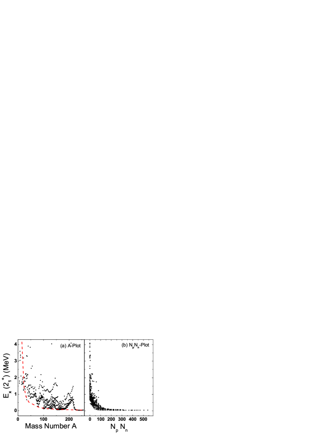
Figure 1: A typical example demonstrating the $N_{p}N_{n}$ scheme. The excitation energies of the first $2^{+}$ states in even-even nuclei are plotted (a) against the mass number $A$ and (b) against the product $N_{p}N_{n}$. The dashed curve in part (a) represents the bottom contour line which is drawn by the first term $\alpha A^{-\gamma}$ of Eq. (1). The excitation energies are quoted from Ref. 4.

The valence nucleon numbers $N_{p}$ and $N_{n}$ have been frequently adopted in parameterizing various nuclear properties phenomenologically over more than the past four decades. Hamamoto was the first to point out that the square roots of the ratios of the measured and the single particle $B(E2)$ values were proportional to the product $N_{p}N_{n}$ Hamamoto . It was subsequently shown that a very simple pattern emerged whenever the nuclear data concerning the lowest collective states was plotted against $N_{p}N_{n}$ Casten1 . This phenomenon has been called the $N_{p}N_{n}$ scheme in the literature Casten2 . For example, when the measured excitation energies $E_{x}(2_{1}^{+})$ of the first excited $2^{+}$ states in even-even nuclei were plotted against the mass number $A$ ($A$-plot), we got data points scattered irregularly over the $E_{x}$-$A$ plane as seen in Fig. 1(a). However, we suddenly had a very neat rearrangement of the data points by just plotting them against the product $N_{p}N_{n}$ ($N_{p}N_{n}$-plot) as shown in Fig. 1(b). A similar simplification was observed not only from $E_{x}(2_{1}^{+})$ but also from the ratio $E_{x}(4_{1}^{+})/E_{x}(2_{1}^{+})$ Casten3 ; Casten4 ; Casten5 , the transition probability $B(E2;2_{1}^{+}\rightarrow 0^{+})$ Casten6 , and the quadrupole deformation parameter $e_{2}$ Casten7 .

The chief attraction of the $N_{P}N_{n}$ scheme is twofold. One is the fact that the simplification in the graph occurs marvelously every time the $N_{p}N_{n}$ plot is drawn. The other attraction is the universality of the pattern, namely the exactly same sort of graphs appears even at different mass regions Casten1 . Since the performance of the $N_{p}N_{n}$ scheme has been so impressive, many expected that the residual valence proton-neutron (p-n) interaction must have been the dominant controlling factor in the development of collectivity in nuclei and that the product $N_{p}N_{n}$ may represent an empirical measure of the integrated valence p-n interaction strength Casten2 . Also, the importance of the p-n interaction in determining the structure of nuclei has long been pointed out by many authors deShalit ; Talmi ; Heyde ; Casten8 ; Zhang ; Federmann ; Dobaczewski .

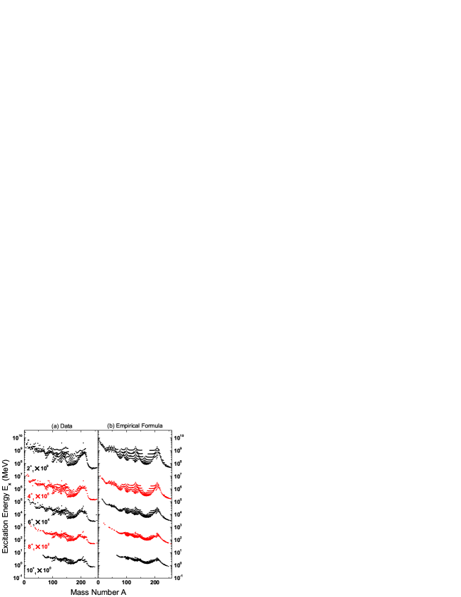
Figure 2: Excitation energies of the first excited natural parity even multipole states. Part (a) shows the measured excitation energies while part (b) shows those calculated by the empirical formula given by Eq. (1). The measured excitation energies are quoted from the compilation in Raman et al. for $2_{1}^{+}$ states Raman and extracted from the Table of Isotopes, 8th-edition by Firestone et al. for other multipole states Firestone .

In the meantime, we have recently proposed a simple empirical formula which describes the essential trends of the excitation energies $E_{x}(2_{1}^{+})$ in even-even nuclei throughout the periodic table Ha1 . This formula, which depends on the valence nucleon numbers, $N_{p}$ and $N_{n}$, and the mass number $A$, can be expressed as

$$E_{x}=\alpha A^{-\gamma}+\beta\left[\exp(-\lambda N_{p})+\exp(-\lambda N_{n})\right]$$ (1)

where the parameters $\alpha$, $\beta$, $\gamma$, and $\lambda$ are fitted from the data. We have also shown that the source, which governs the $2_{1}^{+}$ excitation energy dependence given by Eq. (1) on the valence nucleon numbers, is the effective particle number participating in the residual interaction from the Fermi level Ha2 . Furthermore, the same empirical formula can be applied quite successfully to the excitation energies of the lowest natural parity even multipole states such as $4_{1}^{+}$, $6_{1}^{+}$, $8_{1}^{+}$, and $10_{1}^{+}$ Kim . It can be confirmed by Fig. 2 where the measured excitation energies in part (a) are compared with those in part (b) which are calculated by Eq. (1). The values of the parameters adopted for Fig. 2(b) are listed in Table 1.

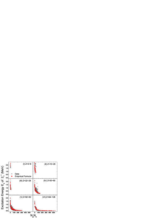
Figure 3: The $N_{p}N_{n}$-plot for the excitation energies of the first $2^{+}$ states using both the data (open triangles) and the empirical formula (solid circles). The plot is divided into six panels each of which contains plotted points that come from each one of the proton major shells.

In this study, we want to further elucidate about our examination of the $N_{p}N_{n}$ scheme based on the empirical formula, Eq. (1), for $E_{x}(2_{1}^{+})$. Our goal is to clarify why $E_{x}(2_{1}^{+})$ complies with the $N_{p}N_{n}$ scheme although the empirical formula, which reproduces the data quite well, does not depend explicitly on the product $N_{p}N_{n}$.

Table 1: Values adopted for the four parameters in Eq. (1) for the excitation energies of the following multipole states: $2_{1}^{+}$, $4_{1}^{+}$, $6_{1}^{+}$, $8_{1}^{+}$, and $10_{1}^{+}$.

Multipole	$\alpha$(MeV)	$\beta$(MeV)	$\gamma$	$\lambda$
$2_{1}^{+}$	34.9	1.00	1.19	0.36
$4_{1}^{+}$	94.9	1.49	1.15	0.30
$6_{1}^{+}$	441.4	1.51	1.31	0.25
$8_{1}^{+}$	1511.5	1.41	1.46	0.19
$10_{1}^{+}$	2489.0	1.50	1.49	0.17

Table 2: The maximum value of $N_{p}N_{n}$ and the minimum value of $E_{x}$ for each major shell in Fig. 3 are indicated here. The numbers in the parenthesis represent $E_{x}$ calculated by the empirical formula given by Eq. (1).

Major Shell	$Z$	Max. $N_{p}N_{n}$	Min. $E_{x}$ (MeV)
I	$2\sim 8$	$8$	$1.59\,(1.85)$
II	$10\sim 20$	$36$	$0.67\,(0.82)$
III	$22\sim 28$	$16$	$0.75\,(0.77)$
IV	$30\sim 50$	$140$	$0.13\,(0.18)$
V	$52\sim 82$	$308$	$0.07\,(0.08)$
VI	$84\sim 126$	$540$	$0.04\,(0.05)$

First, we check how well the empirical formula does meet the requirements of the $N_{p}N_{n}$ scheme. In Fig. 3, we display the $N_{p}N_{n}$-plot for the excitation energies of the first $2^{+}$ states using both the data (empty triangles) and the empirical formula (solid circles). We show them with six panels. Each panel contains plotted points from nuclei which make up the following six different proton major shells: (I) $2\leq Z\leq 8$, (II) $10\leq Z\leq 20$, (III) $22\leq Z\leq 28$, (IV) $30\leq Z\leq 50$, (V) $52\leq Z\leq 82$, and (VI) $84\leq Z\leq 126$. From this figure, we can see an intrinsic feature of the $N_{p}N_{n}$-plot, namely, the plotted points have their own typical location in the $E_{x}$-$N_{p}N_{n}$ plane according to which major shell they belong. For example, the plotted points of the first three major shells I, II, and III occupy the far left side part of the $E_{x}$-$N_{p}N_{n}$ plane in Fig. 3 since their value of the product $N_{p}N_{n}$ does not exceed several tens. On the contrary, the plotted points of the last major shell VI extend to the far right part of the $E_{x}$-$N_{p}N_{n}$ plane along the lowest portion in Fig. 3. This is true since their value of the excitation energy $E_{x}$ is very small and also their value of $N_{p}N_{n}$ reaches more than five hundreds. We present specific information such as the maximum value of $N_{p}N_{n}$ and the minimum value of $E_{x}$ in Table 2 for the plotted points which belong to each major shell in Fig. 3. There are two numbers for each major shell in the last column of Table 2 where one number is determined from the data and the other number in parenthesis is calculated by the empirical formula. We can find that those two numbers agree reasonably well. We also find in Fig. 3 that the results, calculated by the empirical formula (solid circles), meet the requirement of the $N_{p}N_{n}$ scheme very well and agree with the data (empty triangles) satisfactorily for each and every panel.

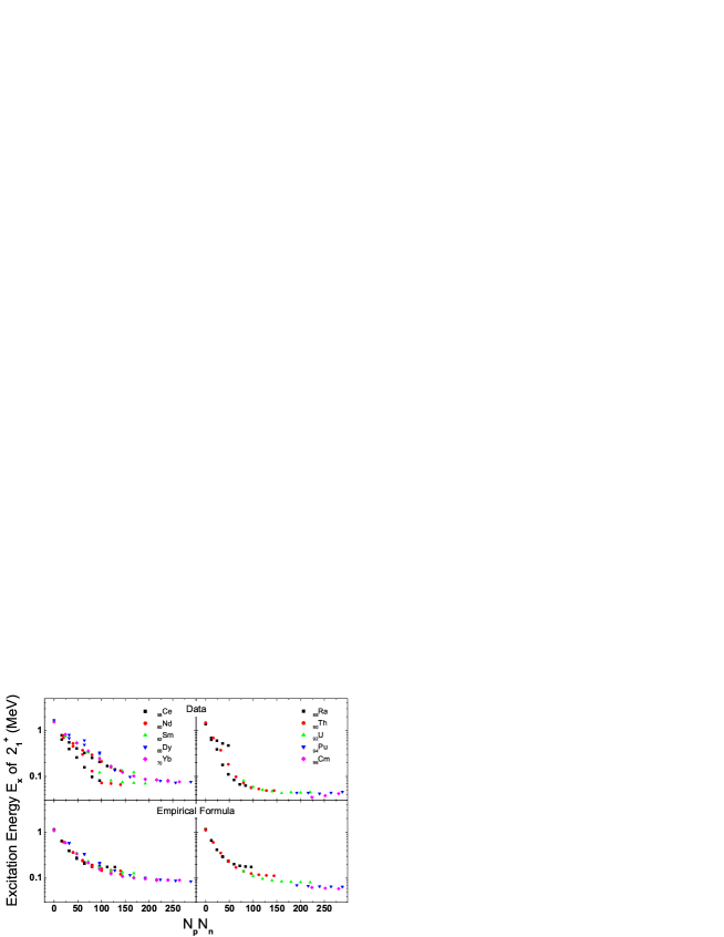
Figure 4: Extract from Fig. 3 for some typical nuclei which belong to the rare earth elements. Different symbols are used to denote excitation energies of individual nuclei.

In order to make more detailed comparison between the measured and calculated excitation energies, we expand the largest two major shells V and VI of Fig. 3 and redraw them in Fig. 4 for some typical nuclei which belong to the rare earth elements. The upper part of Fig. 4 shows the data and the lower part of the same figure exhibits the corresponding calculated excitation energies. We can confirm that the agreement between them is reasonable even though the calculated excitation energies somewhat overestimate the data and also the empirical formula can not separate enough to distinguish the excitation energies of the two isotopes with the same value of the product $N_{p}N_{n}$ for some nuclei.

According to the empirical formula given by Eq. (1), the excitation energy $E_{x}$ is determined by two components: one is the first term $\alpha A^{-\gamma}$ which depends only on the mass number $A$ and the other is the second term $\beta[\exp(-\lambda N_{p})+\exp(-\lambda N_{n})]$ which depends only on the valence nucleon numbers, $N_{p}$ and $N_{n}$. Let us first draw the $N_{p}N_{n}$-plot of $E_{x}(2_{1}^{+})$ by using only the first term $\alpha A^{-\gamma}$. The results are shown in Fig. 5(a) where we can find that the plotted points fill the lower left corner of the $E_{x}$-$N_{p}N_{n}$ plane leaving almost no empty spots. These results simply reflect the fact that a large number of nuclei with different mass numbers, values of $A$, can have the same value of $N_{p}N_{n}$. Now we draw the same $N_{p}N_{n}$-plot by using both of the two terms in Eq. (1). We display the plot of the calculated excitation energies in Fig. 5(b) which is just the same sort of graph of the measured excitation energies shown in Fig. 1(b) except that the type of scale for $E_{x}$ is changed from linear to log. By comparing Fig. 5 (a) and (b), we find that the second term of Eq. (1), which depends on the valence nucleon numbers, $N_{p}$ and $N_{n}$, pushes the plotted points up in the direction of higher excitation energies and arranges them to comply with the $N_{p}N_{n}$ scheme.

It is worthwhile to note the difference between the $A$-plot and the $N_{p}N_{n}$-plot. The graph drawn by using only the first term of Eq. (1) becomes a single curve in the $A$-plot as shown in Fig. 1(a) with the dashed curve. It becomes scattered plotted points in the $N_{p}N_{n}$-plot as can be seen from Fig. 5(a). Now, by adding the second term of Eq. (1) in the $A$-plot, the plotted points are dispersed as shown in the top graph of Fig. 2(b) which corresponds to the measured data points in Fig. 1(a); while by adding the same second term in $N_{p}N_{n}$-plot, we find a very neat rearrangement of the plotted points as shown in Fig. 5(b). Thus, the same second term plays the role of spreading plotted points in the $A$-plot while it plays the role of collecting them in the $N_{p}N_{n}$-plot.

Figure 5: The $N_{p}N_{n}$-plot of the calculated first excitation energy $E_{x}$ of $2^{+}$ states. The excitation energies $E_{x}$ are calculated by (a) using only the first term and (b) using both terms of Eq. (1).

However, this mechanism of the second term alone is not sufficient to explain why the empirical formula given by Eq. (1) which obviously does not depend on $N_{p}N_{n}$ at all, can show the characteristic feature of the $N_{p}N_{n}$ scheme. In order to shed light on this question, we calculate the excitation energy $E_{x}(2_{1}^{+})$ by the following three different conditions on the exponents, $N_{p}$ and $N_{n}$, of the second term in Eq. (1). First, let $N_{p}$ and $N_{n}$ have any even numbers as long as they satisfy $N_{p}+N_{n}\leq A$. The resulting excitation energy $E_{x}$ is plotted against $N_{p}N_{n}$ in Fig. 6(a). Next, let $N_{p}$ and $N_{n}$ have any numbers that are allowed for the valence nucleon numbers. For example, suppose the three numbers of a plotted point are $A=90$, $N_{p}=40$, and $N_{n}=50$ in the previous case. For the fourth major shell IV in Table 2, the valence proton number for the nucleus with the atomic number $Z=40$ is 10 and the valence neutron number for the nucleus with the neutron number $N=50$ is 0. Therefore, we assign $N_{p}=10$ and $N_{n}=0$ instead of 40 and 50, respectively. The excitation energy $E_{x}$, calculated under such a condition, is plotted against $N_{p}N_{n}$ in Fig. 6(b). Last, we take only those excitation energies which are actually measured among the excitation energies shown in Fig. 6(b). The results are shown in Fig. 6(c), which is, of course, exactly the same as shown in Fig. 5(b). From Fig. 6(d) where all the three previous plots (a), (b), and (c) are placed together, we can observe how the $N_{p}N_{n}$ scheme emerges from the empirical formula given by Eq. (1) even though this equation does not depend on the product $N_{p}N_{n}$ at all. On one hand, the two exponential terms which depend on $N_{p}$ and $N_{n}$ separately push the excitation energy $E_{x}$ upward as discussed with respect to Fig. 5. On the other hand, the restriction on the values of the valence nucleon numbers $N_{p}$ and $N_{n}$ of the actually existing nuclei determines the upper bound of the excitation energy $E_{x}$ as discussed regarding Fig. 6.

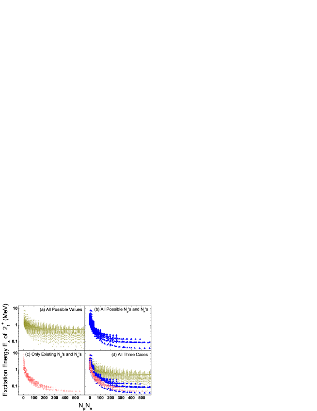
Figure 6: The $N_{p}N_{n}$-plot of the first excitation energy of the $2^{+}$ states calculated by the empirical formula given by Eq. (1) using the following three different conditions on the exponent $N_{p}$ and $N_{n}$: (a) $N_{p}$ and $N_{n}$ can have any even numbers as long as they satisfy $N_{p}+N_{n}\leq A$. (b) $N_{p}$ and $N_{n}$ can have any number that is allowed for the valence nucleon numbers. (c) $N_{p}$ and $N_{n}$ can have numbers which are allowed for the actually existing nuclei. (d) All of the previous three cases are shown together.

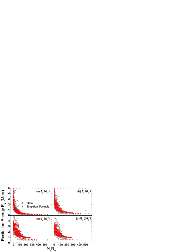
Figure 7: The $N_{p}N_{n}$-plot for the first excitation energies of the natural parity even multipole states (a) $4_{1}^{+}$, (b) $6_{1}^{+}$, (c) $8_{1}^{+}$, and (d) $10_{1}^{+}$ using both the measured data (open triangles) and the empirical formula (solid circles). These graphs are just the $N_{p}N_{n}$-plot versions of the $A$-plot shown in Fig. 2 with exactly the same set of data points.

Finally, we show the $N_{p}N_{n}$-plots of the first excitation energies for (a) $4_{1}^{+}$, (b) $6_{1}^{+}$, (c) $8_{1}^{+}$, and (d) $10_{1}^{+}$ states in Fig. 7. The measured excitation energies are represented by the empty triangles and the calculated ones from the empirical formula, Eq. (1), are denoted by solid circles. These graphs are just the $N_{p}N_{n}$-plot versions of the $A$-plot shown in Fig. 2 with exactly the same set of plotted points. We can learn from Fig. 7 that the same kind of $N_{p}N_{n}$ scheme observed in the excitation energy of $2_{1}^{+}$ states is also functioning in the excitation energies of other natural parity even multipole states. We can also find from Fig. 7 that the calculated results, using the empirical formula, agree with the measured data quite well. Moreover, it is interesting to find from Fig. 7 that the width in the central part of the $N_{p}N_{n}$-plot is enlarged as the multipole of the state is increased. The origin of this enlargement in the empirical formula can be traced to the parameter $\alpha$ of the first term in Eq. (1). The value of $\alpha$ is monotonously increased from $34.9\,{\rm MeV}$ for $E_{x}(2_{1}^{+})$ to $2489.0\,{\rm MeV}$ for $E_{x}(10_{1}^{+})$ as can be seen in Table 1.

In summary, we have examined how the recently proposed empirical formula, Eq. (1), for the excitation energy $E_{x}(2_{1}^{+})$ of the first $2_{1}^{+}$ state meets the requirement of the $N_{p}N_{n}$ scheme even though it does not depend on the product $N_{p}N_{n}$ at all. We have demonstrated explicitly that the structure of the empirical formula itself together with the restriction on the values of the valence nucleon numbers $N_{p}$ and $N_{n}$ of the actually existing nuclei make the characteristic feature of the $N_{p}N_{n}$ scheme appear. Furthermore, our result shows that the composition of the empirical formula, Eq. (1), is in fact ideal for revealing the $N_{p}N_{n}$ scheme. Therefore it is better to regard the $N_{p}N_{n}$ scheme as a strong signature suggesting that this empirical formula is indeed the right one. As a matter of fact, this study about the $N_{p}N_{n}$ scheme has incidentally exposed the significance of the empirical formula given by Eq. (1) as a universal expression for the lowest collective excitation energy. A more detailed account of the empirical formula for the first excitation energy of the natural parity even multipole states in even-even nuclei will be published elsewhere Kim . However, it has been well established that the $N_{p}N_{n}$ scheme holds not only for the lowest excitation energies $E_{x}(2_{1}^{+})$ but also for the transition strength $B(E2)$ Casten6 . Unfortunately, our empirical study intended to express only the excitation energies in terms of the valence nucleon numbers. The extension of our study to include the $B(E2)$ values in our parametrization is in progress.

- (1) I. Hamamoto, Nucl. Phys. 73, 225 (1965).
- (2) R. F. Casten, Nucl. Phys. A443, 1 (1985).
- (3) For a review of the scheme, see R. F. Casten and N. V. Zamfir, J. Phys. G22, 1521 (1996).
- (4) S. Raman, C. W. Nestor, Jr., and P. Tikkanen, At. Data Nucl. Data Tables 78, 1 (2001).
- (5) R. F. Casten, Phys. Rev. Lett. 54, 1991 (1985).
- (6) R. F. Casten, D. S. Brenner, and P. E. Haustein, Phys. Rev. Lett. 58, 658 (1987).
- (7) R. B. Cakirli and R. F. Casten, Phys. Rev. Lett. 96, 132501 (2006).
- (8) R. F. Casten and N. V. Zamfir, Phys. Rev. Lett. 70, 402 (1993).
- (9) Y. M. Zhao, R. F. Casten, and A. Arima, Phys. Rev. Lett. 85, 720 (2000).
- (10) A. de-Shalit and M. Goldhaber, Phys. Rev. 92, 1211 (1953).
- (11) I. Talmi, Rev. Mod. Phys. 34, 704 (1962).
- (12) K. Heyde, P. Vanisacker, R. F. Casten, and J. L. Wood, Phys. Lett. 155B, 303 (1985).
- (13) R. F. Casten, K. Heyde, and A. Wolf, Phys. Lett. 208B, 33 (1988).
- (14) J.-Y. Zhang, R. F. Casten, and D. S. Brenner, Phys. Lett. 227B, 1 (1989).
- (15) P. Federmann and S. Pittel, Phys. Lett. 69B, 385 (1977).
- (16) J. Dobaczewski, W. Nazarewicz, J. Skalski, and T. Werner, Phys. Rev. Lett. 60, 2254 (1988).
- (17) E. Ha and D. Cha, J. Korean Phys. Soc. 50, 1172 (2007).
- (18) E. Ha and D. Cha, Phys. Rev. C 75, 057304 (2007).
- (19) D. Kim, E. Ha, and D. Cha, arXiv:0705.4620[nucl-th].
- (20) R. B. Firestone, V. S. Shirley, C. M. Baglin, S. Y. Frank Chu, and J. Zipkin, Table of Isotopes (Wiley, New York, 1999).