Effects of accelerating growth on the evolution of weighted complex networks

Abstract

Many real systems possess accelerating statistics where the total number of edges grows faster than the network size. In this paper, we propose a simple weighted network model with accelerating growth. We derive analytical expressions for the evolutions and distributions for strength, degree, and weight, which are relevant to accelerating growth. We also find that accelerating growth determines the clustering coefficient of the networks. Interestingly, the distributions for strength, degree, and weight display a transition from scale-free to exponential form when the parameter with respect to accelerating growth increases from a small to large value. All the theoretical predictions are successfully contrasted with numerical simulations.

1 Introduction

Standard interesting objects in the network science are relatively simple binary (Boolean) networks where edges (links) are either present or absent, represented as binary states [1, 2, 3]. In other words, edges in Boolean networks have equal “weights”. However, the connections in many real networks are not homogeneous [4], which naturally calls for a typical measurement of the edge weight, such as the number of joint papers of two coauthors in scientific collaboration network [5, 6, 7, 8], the number of flights or seats between any two cities in airline networks [9, 10], the bandwidth of a link in the Internet [11], the reaction rate in metabolic network [12], and so on. These real systems with diversity of edges can be better described in terms of weighted networks.

Various weighted network models have been proposed to describe and explain the real-life systems [4]. Yook et al. took a first step in the direction of a model study for evolving weighted network (YJBT model) [13], where the topology and weight are driven by only the network connection based on preferential attachment (PA) rule [14]. The YJBT model overlooks the possible dynamical evolution and reinforcements of weights, which is a common property of real-life networks [4]. To better mimic the reality, Barrat, Barthélemy, and Vespignani presented a growing model (BBV) for weighted networks, where the evolutions of degree and weight are coupled [15, 16]. Enlightened by BBV’s remarkable work, a variety of models and mechanisms for weighted networks have been proposed, including weight-driven model [17], traffic-driven evolution models [18, 19], fitness models [20], local-world models [21, 22, 23], deterministic models [24, 25, 26], weight-dependent deactivation [27], spatial constraints [28, 29].

Recent empirical study demonstrated that many real natural and social networks exhibit the characteristic of “accelerating growth”, which means that the total number of edges increases more quickly than linearly with the node (vertex) number. Generally, networks with this property are called “accelerating networks”. For instance, in both the World Wide Web [30] and the Internet [11] the number of edges increases with time in a nonlinear fashion. In metabolic network [12], the total number of links exceeds the total number of nodes by about an order of magnitude. Other familiar examples of accelerating networks include scientific collaboration network [5, 6, 7, 8], language network [31], citation network [32], etc. Inspired by this phenomenon, the research on accelerating networks has attracted an amount of attention [33, 34, 35, 36, 37].

Actually, accelerating networks are far more common in the real world than has hitherto been appreciated [35]. Despite their widespread appearance, evolving weighted networks with accelerating growth have received less attention. This important factor of accelerating growth is neglected in most of the considered weighted network models [13, 15, 16, 17, 18, 19, 20, 21, 24, 25, 26, 27, 28, 29]. Then questions arise naturally: Can an accelerating growth model for weighted networks be established? How much effect does the accelerating growth have on the evolution of weighted networks?

In this paper, we present an accelerating weighted network model to understand how the accelerating growth phenomenon affects the dynamical evolution of weighted networks. We study both analytically and numerically the network characteristics, including the evolution and distributions of the degree, weight, and strength, as well as the clustering coefficient. We show that obtained properties depend on the accelerating parameter.

2 Definitions

We give a brief introduction to the definitions of tools for statistical characterization of weighted networks.

Mathematically, for a weighted network, its topological as well as weighted properties can be completely described by a generalized adjacency matrix $W$, whose element $w_{ij}$ specifies the weight of the edge between node $i$ and $j$. $w_{ij}=0$ represents that node $i$ and $j$ are disconnected. In the following, we focus on the cases of undirected graphs, which have symmetric nonnegative weights $w_{ij}=w_{ji}\geq 0$. Moreover, we assure that $w_{ii}=0$.

The standard topological characterization of binary networks is also applied for weighted networks, which is obtained by the analysis of the distribution $P(k)$ that represents the probability of a random selected node to have degree $k$. In a weighted network, a natural generalization of degree is the node strength defined as $s_{i}=\sum_{j\in\Gamma(i)}w_{ij}$, where the sum runs over the set $\Gamma(i)$ of neighbors of the node $i$. Statistical properties of weighted networks can be characterized by the distributions of strength $P(s)$ and weight $P(w)$, which denote the probability of a node to have strength $s$ and of an edge to have weight $w$.

3 The model for accelerating weighted networks

The model proposed here begins from an initial configuration of $N_{0}$ nodes connected by edges with assigned weight $w_{0}=1$. At each time step, the network evolves under the following two coupled mechanisms: topological growth and weights’ dynamics.

(i) Topological growth. A new node $n$ enters the network. If the new node is born at time $t$, we assume that the edge number of this new node is a power law function $t^{\theta}$ ($0\leq\theta\leq 1$) depending on time $t$, where $\theta$ is the acceleration parameter. (Since multiple edges are forbidden, the total number of edges is smaller than $t^{2}/2$, thus $\theta$ cannot be greater than 1. On the other hand, when $\theta<0$, the new node may carry no edge, which is not consistent with most real networks. Thus, one may reasonably assume $0\leq\theta\leq 1$.) These $t^{\theta}$ new edges have initial weight $w_{0}=1$ and are randomly attached to a previously existing node $i$ according to the preferential probability

$$\Pi_{n\rightarrow i}=\frac{s_{i}}{\sum_{j}s_{j}}\,,$$ (1)

where the sum runs over all existing nodes.

(ii) Weights’ dynamics. The creation of each of the $t^{\theta}$ edges will introduce variations of the existing weights across the network. For the sake of the simplicity, we only consider the local rearrangements of weights of those edges connecting $i$ and its neighbors $j\in\Gamma(i)$, according to the simple rule

$$w_{ij}\rightarrow w_{ij}+\delta\frac{w_{ij}}{s_{i}}\,.$$ (2)

Here we have assumed the addition of each new edge induces a total increment $\delta$ ($\delta$=const) of weights. The rule described by Eq. (2) yields a global increase of $w_{0}+\delta$ for the strength of node $i$, which will therefore become even more attractive to future nodes.

After updating the weights, the growing process is iterated by introducing another new node, i.e. returning to step (i) until the network reaches the desired size. Since the network size is incremented by one with each time step, we use the step value $t$ to represent the node created at this step. At time $t$, the network has $N=t+N_{0}$ nodes and $\int t^{\theta}dt=t^{1+\theta}/(1+\theta)$ edges in the continuum limit.

Note that many real-life networks exhibit such an evolving mechanism as described in our model. Mechanism (i) is a plausible one that appears in many real systems such as the Internet and scientific collaboration networks; it corresponds to the fact that new nodes try to connect a preexisting node with a probability proportional to the strength of the old node, as provided by Eq. (1). An important aspect of mechanism (i) is that the number of edges carried by the new node is not a constant, but controlled by a parameter $\theta$ $(0\leq\theta\leq 1)$, which we call accelerating exponent. This has been confirmed by a variety of empirical observations. For example, for arXiv citation graph, autonomous system graph of the Internet, and the email networks, their accelerating exponents have been found to be 0.56, 0.18, and 0.12, respectively [38]. On the other hand, mechanism (ii) describes the weight dynamics induced by a new edge onto the old ones, which can happen in scientific collaboration networks, airline networks, and so on. See Refs. [9, 15, 16] for detailed explanation.

The model is governed by two parameters $\delta$ and $\theta$, according to which there are some limiting cases of the model. When $\delta=0$ and $\theta=0$, it is reduced to the BA model [14]. For $\theta=0$, it coincides with a special case of the BBV model [15, 16]. Varying $\delta$ and $\theta$ allows one to study the crossover between the two limiting models, which have qualitatively different properties from the two limits. We will show that both of the parameters $\delta$ and $\theta$ have significant effects on the network evolution, here we focus on the latter that has never been studied before, while the former has been discussed in Ref. [16].

4 Evolution and distributions of strength, degree and weight

Our growing model can be studied analytically through the time evolution of the average value of $s_{i}(t)$ and $k_{i}(t)$ of the $i$th node at time $t$ by using the “mean-field” method. According to the evolution rules, the addition of each new edge results in the increase of total network strength by an amount equal to $2+2\delta$. Thus, after $t$ steps of evolution, the total strength of the network is obtained to be

$$\sum_{i}s_{i}(t) =\sum_{i=0}^{t}i^{\theta}(2+2\delta)$$ (3)

$$\approx\int_{0}^{t}i^{\theta}(2+2\delta)di$$

$$=\frac{2(1+\delta)}{\theta+1}t^{\theta+1}\,.$$

When a new node $n$ enters the network, an existing node $i$ can be affected in two ways: (1) The new node is connected to $i$ with probability given by Eq. (1), thus the degree and strength of $i$ are increased by 1 and $1+\delta$, respectively. (2) The new node is connected to one of $i$’s neighbors $j\in\Gamma(i)$, in this case the degree of $i$ remains unmodified, while $w_{ij}$ is increased according to Eq. (2), and thus $s_{i}$ is increased by $\delta w_{ij}/s_{j}$. We assume that variables $s_{i}$ and $k_{i}$ are continuous. Then, at each time step, the strength $s_{i}$ and degree $k_{i}$ of a node evolve as

$$\frac{ds_{i}}{dt} =t^{\theta}\frac{s_{i}}{\sum_{j}s_{j}}(1+\delta)+\sum_{j\in\Gamma(i)}t^{\theta}\frac{s_{j}}{\sum_{k}s_{k}}\delta\frac{w_{ij}}{s_{j}}$$ (4)

$$=\frac{2\delta+1}{2\delta+2}(1+\theta)\frac{s_{i}(t)}{t}\,,$$

and

$$\frac{dk_{i}}{dt}=t^{\theta}\frac{s_{i}(t)}{\sum_{j}s_{j}(t)}=\frac{1+\theta}{2+2\delta}\frac{s_{i}(t)}{t},$$ (5)

respectively.

With the initial conditions $k_{i}(t=i)=s_{i}(t=i)=i^{\theta}$, we can integrate above equations to obtain

$$s_{i}(t)=i^{\theta}\left(\frac{t}{i}\right)^{\beta}=i^{\theta}\left(\frac{t}{i}\right)^{\frac{(2\delta+1)(1+\theta)}{2\delta+2}},$$ (6)

and

$$k_{i}(t) =\frac{s_{i}(t)+2\delta t^{\theta}}{2\delta+1}$$ (7)

$$=\frac{i^{\theta}\left(\frac{t}{i}\right)^{\frac{(2\delta+1)(1+\theta)}{2\delta+2}}+2\delta t^{\theta}}{2\delta+1}.$$

For large $t$, it can be always guaranteed that $s_{i}(t)$ is larger than $2\delta t^{\theta}$ because one can easily see that $\frac{(2\delta+1)(1+\theta)}{2\delta+2}>\theta$ given $\theta\in[0,1]$ and $\delta>0$. Thus, $s_{i}(t)$ and $k_{i}(t)$ are proportional when $t$ is large. From the obtained expressions, we find that dynamical exponent $\beta=\frac{(2\delta+1)(1+\theta)}{2\delta+2}$ depends on not only $\delta$, but also $\theta$, which is significantly different from the BBV model and BA network. Figure 1 shows the behavior of the nodes’ degree and strength versus time for different $\theta$, which recovers the results predicted analytically.

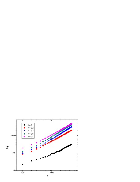
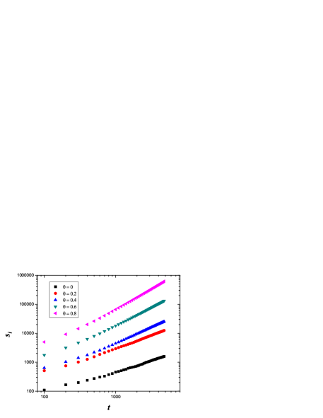
Figure 1: (Color online) Time-evolution for the degree and strength of nodes, added to the systems started at $t=1$ in the case of $\delta=2$.

We assume that the nodes are added to the systems at equal time intervals, then the probability that a node has strength $s_{i}(t)$ smaller than $s$, $P(s_{i}(t)<s)$, can be written as

$$P\left(s_{i}(t)<s\right) = P\left(i>s^{-\frac{2\delta+2}{2\delta+1-\theta}}t^{\frac{(2\delta+1)(1+\theta)}{2\delta+1-\theta}}\right)$$ (8)

$$= 1-P\left(i\leq s^{-\frac{2\delta+2}{2\delta+1-\theta}}t^{\frac{(2\delta+1)(1+\theta)}{2\delta+1-\theta}}\right)$$

$$= 1-\frac{1}{N_{0}+t}s^{-\frac{2\delta+2}{2\delta+1-\theta}}t^{\frac{(2\delta+1)(1+\theta)}{2\delta+1-\theta}}.$$

The probability distribution of strength $P(s)$ can be calculated through solving the partial differentiation of $P(s_{i}(t)<s)$ on $s$, and the final result of strength distribution at time $t$ exhibits the following behavior:

$$P(s)=\frac{2\delta+2}{2\delta+1-\theta}f(t)s^{-\frac{4\delta+3-\theta}{2\delta+1-\theta}},$$ (9)

where $f(t)=\frac{1}{t+N_{0}}\,t^{(2\delta+1)(1+\theta)/(2\delta+1-\theta)}$. Therefore, the strength follows a power law distribution with an exponent

$$\gamma_{s}=\frac{4\delta+3-\theta}{2\delta+1-\theta}\,.$$ (10)

Since there is an approximatively linear relationship between the degree and strength for the same node, the degree distribution $P(k)$ has also a scale-free form, $P(k)\sim k^{-\gamma_{k}}$ with the exponent $\gamma_{k}$ identical to $\gamma_{s}$.

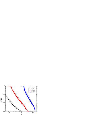
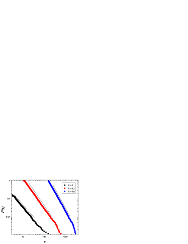
Figure 2: (Color online) The cumulative distributions of nodes’ degree and strength at various $\theta$ values for $\delta=5$. The network size is $N=5000$, and the straight lines are the theoretical results of $\gamma_{k,cum}=\gamma_{s,cum}=(4\delta+3-\theta)/(2\delta+1-\theta)-1$.

In order to confirm the validity of the obtained analytical predictions, we performed extensive numerical simulations of the networks. To reduce the effect of fluctuation on simulation results, the simulation results are average over ten network realizations. Figure 2 gives the accumulative distributions of nodes’ degree and strength. Numerical results are consistent with the theoretical ones.

Now we investigate the evolution of the weights $w_{ij}$ with time, which can also be computed analytically using mean field approximation employed for the research of $s_{i}(t)$ and $k_{i}(t)$. During the process of network growth, $w_{ij}$ can only increase by the addition of a new node connected to either node $i$ or $j$, and the evolution of $w_{ij}$ satisfies the following equation

$$\frac{dw_{ij}}{dt} =t^{\theta}\frac{s_{i}}{\sum_{k}s_{k}}\delta\frac{w_{ij}}{s_{i}}+t^{\theta}\frac{s_{j}}{\sum_{k}s_{k}}\delta\frac{w_{ij}}{s_{j}}$$ (11)

$$=\frac{\delta(1+\theta)}{1+\delta}\frac{w_{ij}}{t}.$$

The edge $(i,j)$ is built only when both node $i$ and $j$ have been created, therefore the birth time of edge $(i,j)$ is $t_{ij}=max(i,j)$. Considering the initial condition $w_{ij}=1$, one can integrate the Eq. (11) to obtain

$$w_{ij}(t)=\left(\frac{t}{t_{ij}}\right)^{\frac{\delta(1+\theta)}{\delta+1}},$$ (12)

which implies that the edge weight $w$ displays a power-law distribution, $P(w)\sim w^{-\gamma_{w}}$, with the exponent $\gamma_{w}=\frac{1+2\delta+\delta\theta}{(1+\theta)\delta}$. To check the validity of the analytical predictions for the evolution and distribution of the edge weight, we have performed numerical simulations of the present model, which are plotted in Fig. 3. The simulations are in agreement with the analytical calculations.

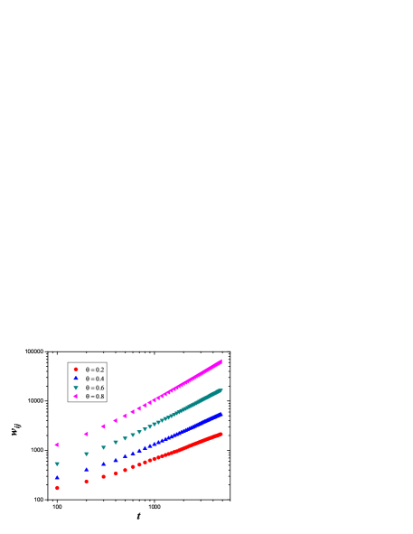
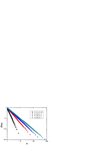
Figure 3: (Color online) (Upper panel) Log-log plot of time-evolution for the weight of edges, which are born at step $t=1$ in the case of $\delta=2$. (Lower panel) The cumulative distribution of edge weight for network size $N=5000$ at different $\theta$ and $\delta$. The dashed straight lines are the theoretical results of $\gamma_{w,cum}=(1+2\delta+\delta\theta)/[(1+\theta)\delta]-1$.

So far, we have shown that the considered accelerating weighted network has power-law distributions of strength, degree, and weight. All the obtained exponents $\gamma_{k}=\gamma_{s}=\frac{4\delta+3-\theta}{2\delta+1-\theta}$, and $\gamma_{w}=\frac{1+2\delta+\delta\theta}{(1+\theta)\delta}$ vary from 2 to $\infty$, depending on the network parameters $\delta$ and $\theta$. It should be noted that in the BBV model, where $\theta$ equals zero, exponents $\gamma_{k}=\gamma_{s}$ are between 2 and 3. Thus, accelerating growth has an important effect on the evolution of the network: when $\theta$ increases from 0 to 1, distributions of strength, degree, and weight exhibit a transition from scale-free (small exponent) to exponential (large exponent) forms. Moreover, by tuning the values of parameter $\theta$, the network may have different forms of degree (strength) distribution and weight distribution. For example, when $\delta\to 0$, the exponents $\gamma_{k}$ ($\gamma_{s}$) and $\gamma_{w}$ are reduced to $\gamma_{k}=\gamma_{s}=1+\frac{2}{1-\theta}$ and $\gamma_{w}=\infty$, respectively. In this case, the weight distribution is always exponential, while the degree (strength) distribution follows a power-law form with $\gamma_{k}$ ($\gamma_{s}$) increasing from 3 to $\infty$ when parameter $\theta$ increases from 0 to 1.

5 Clustering coefficient

As studied in the previous section, accelerating growth significantly affects the network properties, such as distributions of strength, degree, and weight. In this section, we will show that the parameter $\theta$ concerning accelerating growth also controls the clustering coefficient of the networks.

By definition, the clustering coefficient [39] of a given node is the ratio of the total number of edges that actually exist between all its $k$ nearest neighbors and the potential number of edges $k(k-1)/2$ between them. The clustering coefficient of the whole network is obtained through averaging over all its nodes.

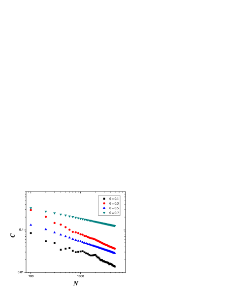
Figure 4: (Color online) Average clustering coefficient $C$ vs parameter $\theta$ and the network size $N$. All data are from the average of ten independent simulations for the same network.

We have performed numerical simulations of the networks to study the influence of the acceleration parameter $\theta$ on clustering coefficient, which is presented in Fig. 4. Numerical simulation results show that for arbitrary $\theta$, the average clustering coefficient $C(N)$ decreases as the size increases, i.e. $C(N)\sim N^{-\eta}$, as reported in Fig. 4. This power-law behavior is similar to that of Barabási-Albert (BA) model [1], and is in contrast to the observation of some real networks such as the Internet and metabolic networks whose clustering coefficient is independent of their size [40]. However, to the best of our knowledge, whether there is real networks exhibiting similar phenomenon of clustering coefficient as our model is still unknown, which deserves further study in future.

In fact, there are two known limits for the average clustering coefficient $C$ of the whole network: In the case of $\theta=0$, the network is a tree, and hence it has no triangle, therefore $C=0$; when $\theta=1$, the network corresponds to a complete graph (i.e. $N$-clique) with clustering coefficient $C=1$. Figure 4 also shows the dependence of $C$ on $\theta$. One can easily see that $C$ is an increasing function of $\theta$ as expected. The increase is not very sharp for small $\theta$, but we can expect an obvious increase of $C$ for $\theta$ of very large values.

6 Conclusion

In conclusion, we have proposed a growing model for weighted networks in which the number of edges added with each new node is an increasing function (power law function) of network size. We have demonstrated that the accelerating growth is an important factor that establishes the network structure. Using mean field network theory, we have computed analytical expressions for the evolution and distributions of strength, degree and weight. The obtained results show that these distributions are subject to a transition from a power-law to exponential shape, when the acceleration parameter is tuned from a small to large value. All mean field approximations have been confirmed by numerical simulations. Our model may provide valuable insight into the real-life networks.

Although accelerating growth exists in many real-life networks, it should be pointed out that the nonlinear growth fashion of the edges compared with nodes in real systems is more intricate and flexible. We use here the most generic case, i.e. the number of total edges is a power-law function of the total node number. In future, it would be worth studying in detail other manners of nonlinear growth in different real-life networks as well as their impacts on network properties and dynamics.

References

- [1] R. Albert and A.-L. Barabási, Rev. Mod. Phys. 74, 47 (2002).
- [2] S. N. Dorogvtsev and J.F.F. Mendes, Adv. Phys. 51, 1079 (2002).
- [3] M. E. J. Newman, SIAM Review 45, 167 (2003).
- [4] S. Boccaletti, V. Latora, Y. Moreno, M. Chavezf, and D.-U. Hwanga, Phy. Rep. 424, 175 (2006).
- [5] M. E. J. Newman, Proc. Natl. Acad. Sci. U.S.A. 98, 404 (2001).
- [6] M. E. J. Newman, Phys. Rev. E 64, 016132 (2001).
- [7] A.-L. Barabási, H. Jeong, Z. Néda. E. Ravasz, A. Schubert, and T. Vicsek, Physica A 311, 590 (2002).
- [8] M. Li, J. Wu, D. Wang, T. Zhou, Z. Di, Y. Fan, Physica A 375, 355 (2007).
- [9] A. Barrat, M. Barthélemy, R. Pastor-Satorras, and A. Vespignani, Proc. Natl. Acad. Sci. U.S.A. 101, 3747 (2004).
- [10] W. Li, and X. Cai, Phys. Rev. E 69, 046106 (2004).
- [11] M. Faloutsos, P. Faloutsos and C. Faloutsos, Comput. Commun. Rev. 29, 251 (1999).
- [12] H. Jeong, B. Tombor, R. Albert, Z. N. Oltvai and A.-L. Barabási, Nature 407, 651 (2000).
- [13] S. H. Yook, H. Jeong, A.-L. Barabási, Y. Tu, Phys. Rev. Lett. 86, 5835 (2001).
- [14] A.-L. Barabási and R. Albert, Science 286, 509 (1999).
- [15] A. Barrat, M. Barthélemy, and A. Vespignani, Phys. Rev. Lett. 92, 228701 (2004).
- [16] A. Barrat, M. Barthélemy, and A. Vespignani, Phys. Rev. E 70, 066149 (2004).
- [17] T. Antal and P. L. Krapivsky, Phys. Rev. E 71 026103 (2005).
- [18] W.-X. Wang, B.-H. Wang, B. Hu, G. Yan, and Q. Ou, Phys. Rev. Lett. 94, 188702 (2005).
- [19] Y.-B. Xie, W.-X. Wang, and B.-H. Wang, Phys. Rev. E 75, 026111 (2007).
- [20] G. Bianconi, Europhys. Lett. 71, 1029 (2005).
- [21] Z. Pan, X. Li, and X. Wang, Phys. Rev. E 73, 056109 (2006).
- [22] B. Wang, H. W. Tang, Z. Z. Zhang, and Z. L. Xiu, Int. J. Mod. Phys. B 19, 3951 (2005).
- [23] Z.Z. Zhang, L. L. Rong, B. Wang, S. G. Zhou, and J. H. Guan, Physica A 380, 639 (2007).
- [24] S. N. Dorogvtsev and J. F. F. Mendes, AIP Conf. Proc. 776, 29 (2005).
- [25] Z.Z. Zhang, S.G. Zhou, L.J. Fang, J.H. Guan, Y.C. Zhang, EPL 79, 38007 (2007)
- [26] Z.Z. Zhang, S. G. Zhou, L. C. Chen, J. H. Guan, L. J. Fang, and Y. C. Zhang, Eur. Phys. J. B 59, 99 (2007).
- [27] Z.-X. Wu, X.-J. Xu, and Y.-H. Wang, Phys. Rev. E 71, 066124 (2005).
- [28] A. Barrat, M. Barthélemy, and A. Vespignani, J. Stat. Mech: Theory Exp. P05003 (2005).
- [29] G. Mukherjee and S. S. Manna, Phys. Rev. E 74, 036111 (2006).
- [30] A. Broder, R. Kumar, F. Maghoul, P. Raghavan, S. Rajagopalan, R. Stata, A. Tomkins, and J. Wiener, Comput. Netw. 33, 309 (2000).
- [31] S. N. Dorogovtsev and J. F. F. Mendes, Proc. R. Soc. London, Ser. B 268, 2261 (2001)
- [32] S. Redner, Eur. Phys. J. B 4, 131 (1998).
- [33] S. N. Dorogovtsev and J. F. F. Mendes, Phys. Rev. E 63, 025101(R) (2001).
- [34] P. Sen, Phys. Rev. E 69, 046107 (2004).
- [35] J. S. Mattick and M. J. Gagen, Science 307, 856 (2005).
- [36] M. J. Gagen and J. S. Mattick, Phys. Rev. E 72, 016123 (2005).
- [37] X. Yu, Z. Li, D. Zhang, F. Liang, X. Wang, and X. Wu, J. Phys. A 39, 14343 (2006).
- [38] J. Leskovec, J. Kleinberg, C. Faloutsos, ACM Transactions on Knowledge Discovery from Data, 1, 1 (2007).
- [39] D. J. Watts and H. Strogatz, Nature (London) 393, 440 (1998).
- [40] E. Ravasz, A.-L. Barabási, Phys. Rev. E 67, 026112 (2003).