Diffuse Optical Light in Galaxy Clusters II:
Correlations with Cluster Properties

Abstract

We have measured the flux, profile, color, and substructure in the diffuse intracluster light (ICL) in a sample of ten galaxy clusters with a range of mass, morphology, redshift, and density. Deep, wide-field observations for this project were made in two bands at the one meter Swope and 2.5 meter du Pont telescope at Las Campanas Observatory. Careful attention in reduction and analysis was paid to the illumination correction, background subtraction, point spread function determination, and galaxy subtraction. ICL flux is detected in both bands in all ten clusters ranging from $7.6\times 10^{10}$ to $7.0\times 10^{11}$ $h_{70}^{-1}$L_⊙in $r$ and $1.4\times 10^{10}$ to $1.2\times 10^{11}$ $h_{70}^{-1}$L_⊙in the $B-$band. These fluxes account for 6 to 22% of the total cluster light within one quarter of the virial radius in $r$ and 4 to 21% in the $B-$band. Average ICL $B-r$ colors range from 1.5 to 2.8 mags when k and evolution corrected to the present epoch. In several clusters we also detect ICL in group environments near the cluster center and up to  1$h_{70}^{-1}$Mpc distant from the cluster center. Our sample, having been selected from the Abell sample, is incomplete in that it does not include high redshift clusters with low density, low flux, or low mass, and it does not include low redshift clusters with high flux, mass, or density. This bias makes it difficult to interpret correlations between ICL flux and cluster properties. Despite this selection bias, we do find that the presence of a cD galaxy corresponds to both centrally concentrated galaxy profiles and centrally concentrated ICL profiles. This is consistent with ICL either forming from galaxy interactions at the center, or forming at earlier times in groups and later combining in the center.

1 Introduction

A significant stellar component of galaxy clusters is found outside of the galaxies. The standard theory of cluster evolution is one of hierarchical collapse, as time proceeds, clusters grow in mass through the merging with other clusters and groups. These mergers as well as interactions within groups and within clusters strip stars out of their progenitor galaxies. The study of these intracluster stars can inform hierarchical formation models as well as tell us something about physical mechanisms involved in galaxy evolution within clusters.

Paper I of this series (Krick et al., 2006) discusses the methods of ICL detection and measurement as well as the results garnered from one cluster in our sample. We refer the reader to that paper and the references therein for a summary of the history and current status of the field. This paper presents the remaining nine clusters in the sample and seeks to answer when and how intracluster stars are formed by studying the total flux, profile shape, color, and substructure in the ICL as a function of cluster mass, redshift, morphology, and density in the sample of 10 clusters. The advantage to having an entire sample of clusters is to be able to follow evolution in the ICL and use that as an indicator of cluster evolution.

Strong evolution in the ICL fraction with mass of the cluster has been predicted in simulations by both Lin & Mohr (2004) and Murante et al. (2004). If ongoing stripping processes are dominant, ram pressure stripping (Abadi et al., 1999) or harassment (Moore et al., 1996), then high mass clusters should have a higher ICL fraction than low-mass clusters . If, however, most of the galaxy evolution happens early on in cluster collapse by galaxy-galaxy merging, then the ICL should not correlate directly with current cluster mass.

Because an increase in mass is tied to the age of the cluster under hierarchical formation, evolution has also been predicted in the ICL fraction as a function of redshift (Willman et al., 2004; Rudick et al., 2006). Again, if ICL formation is an ongoing process then high redshift clusters will have a lower ICL fraction than low redshift clusters. Conversely, if ICL formation happened early on in cluster formation there will be no correlation of ICL with redshift.

The stripping of stars (or even the gas to make stars) to create an intracluster stellar population requires an interaction between their original host galaxy and either another galaxy, the cluster potential, or possibly the hot gas in the cluster. Because all of these processes require an interaction, we expect cluster density to be a predictor of ICL fraction. Cluster density is linked to cluster morphology, which implies morphology should also be a predictor of ICL fraction. Specifically we measure morphology by the presence or absence of a cD galaxy. cD galaxies are the results of 2 - 5 times more mergers than the average cluster galaxy (Dubinski, 1998). The added number of interactions that went into forming the cD galaxy will also mean an increased disruption rate in galaxies therefore morphological relaxed (dynamically old) clusters should have a higher ICL flux than dynamically young clusters.

Observations of the color and fractional flux in the ICL over a sample of clusters with varying redshift and dynamical state will allow us to identify the timescales involved in ICL formation. If the ICL is the same color as the cluster galaxies, it is likely to be a remnant from ongoing interactions in the cluster. If the ICL is redder than the galaxies it is likely to have been stripped from galaxies at early times. Stripped stars will passively evolve toward red colors while the galaxies continue to form stars. If the ICL is bluer than the galaxies, then some recent star formation has made its way into the ICL, either from ellipticals with low metallicity or spirals with younger stellar populations, or from in situ formation.

While multiple mechanisms are likely to play a role in the complicated process of formation and evolution of clusters, important constraints can come from ICL measurement in clusters with a wide range of properties. In addition to directly constraining galaxy evolution mechanisms, the ICL flux and color is a testable prediction of cosmological models. As such it can indirectly be used to examine the accuracy of the physical inputs to these models.

This paper is structured in the following manner. In §2 we discuss the characteristics of the entire sample. Details of the observations and reduction are presented in §3 and §4 including flat-fielding, sky background subtraction methods, object detection, and object removal and masking. In §5 we lists the results for both cluster and ICL properties including a discussion of each individual cluster. Accuracy limits are discussed in §6. A discussion of the interesting correlations can be found in §7 followed by a summary of the conclusions in §8.

Throughout this paper we use $H_{0}=70$km/s/Mpc, $\Omega_{M}$ = 0.3, $\Omega_{\Lambda}$ = 0.7.

2 The Sample

The general properties of our sample of ten galaxy clusters have been outlined in paper I; for completeness we summarize them briefly here. Our choice of the 10 clusters both minimizes the observational hazards of the galactic and ecliptic plane, and maximizes the amount of information in the literature. All clusters were chosen to have published X–ray luminosities which guarantees the presence of a cluster and provides an estimate of the cluster’s mass. The ten chosen clusters are representative of a wide range in cluster characteristics, namely redshift ($0.05<z<0.3$), morphology (3 with no clear central dominant galaxy, and 7 with a central dominant galaxy as determined from this survey, §5.1.2, and not from Bautz Morgan morphological classifications), spatial projected density (richness class 0 - 3), and X–ray luminosity ($1.9\times 10^{44}$ ergs/s $<Lx<22\times 10^{44}$ ergs/s). We discuss results from the literature and this survey for each individual cluster in order of ascending redshift in §5.

3 Observations

The sample is divided into a “low” ($0.05<z<0.1$) and “high” ($0.15<z<0.3$) redshift range which we have observed with the 1 meter Swope and 2.5 meter du Pont telescope respectively. The du Pont observations were discussed in detail in paper I. The Swope observations follow a similar observational strategy and data reduction process which we outline below. Observational parameters are listed in Table 2.

We used the $2048\times 3150$ “Site#5” CCD with a $3e^{-}/$count gain and $7e^{-}$ readnoise on the Swope telescope. The pixel scale is 0.435″/pixel ($15\mu$ pixels), so that the full field of view per exposure is $14.8\arcmin\times 22.8\arcmin$. Data was taken in two filters, Gunn-$r$ ($\lambda_{0}=6550$ Å) and $B$ ($\lambda_{0}=4300$ Å). These filters were selected to provide some color constraint on the stellar populations in the ICL by spanning the 4000Å break at the relevant redshifts, while avoiding flat-fielding difficulties at longer wavelengths and prohibitive sky brightness at shorter wavelengths.

Observing runs occurred on October 20-26, 1998, September 2-11, 1999, and September 19-30, 2000. All observing runs took place within eight days of new moon. A majority of the data were taken under photometric conditions. Those images taken under non-photometric conditions were individually tied to the photometric data (see discussion in §4. Across all three runs, each cluster was observed for an average of 5 hours in each band. In addition to the cluster frames, night sky flats were obtained in nearby, off-cluster, “blank” regions of the sky with total exposure times roughly equal to one third of the integration times on cluster targets. Night sky flats were taken in all moon conditions. Typical $B-$ and $r-$band sky levels during the run were $22.7$ and $21.0$ mag arcsec^-2, respectively.

Cluster images were dithered by one third of the field of view between exposures. The large overlap from the dithering pattern gives us ample area for linking background values from the neighboring cluster images. Observing the cluster in multiple positions on the chip reduces large-scale flat-fielding fluctuations upon combination. Integration times were typically 900 seconds in $r$ and 1200 seconds in $B$.

4 Reduction

In order to create mosaiced images of the clusters with a uniform background level and accurate resolved–source fluxes, the images were bias and dark subtracted, flat–fielded, flux calibrated, background–subtracted, extinction corrected, and registered before combining. Methods for this are discussed in detail in paper I and summarized below.

The bias level is roughly 270 counts which changed by approximately 8% throughout the night. This, along with the large-scale ramping effect in the first 500 columns of every row was removed in the standard manner using IRAF tasks. The mean dark level is 1.6 counts/900s, and there is some vertical structure in the dark which amounts to 1.4 counts/900s over the whole image. To remove this large-scale structure from the data images, a combined dark frame from the whole run was median smoothed over $9\times 9$ pixels ($3.9\arcsec$), scaled by the exposure time, and subtracted from the program frames. Small scale variations were not present in the dark. Pixel–to–pixel sensitivity variations were corrected in all cluster and night-sky flat images using nightly, high S/N, median-combined dome flats with 70,000 – 90,000 total counts. After this step, a large-scale illumination pattern remains across the chip. This was removed using night-sky flats of “blank” regions of the sky, which, when combined using masking and rejection, produced an image with no evident residual flux from sources but has the large scale illumination pattern intact. The illumination pattern was stable among images taken during the same moon phase. Program images were corrected only with night sky flats taken in conditions of similar moon.

We find that the Site#3 CCD does have an approximately $7\%$ non-linearity over the full range of counts, which we fit with a second order polynomial and corrected for in all the data. The same functional fit was found for both the 1998 and 1999 data, and also applied to the 2000 data. The uncertainty in the linearity correction is incorporated in the total photometric uncertainty.

Photometric calibration was performed in the usual manner using Landolt standards at a range of airmasses. Extinction was monitored on stars in repeat cluster images throughout the night. Photometric nights were analyzed together; solutions were found in each filter for an extinction coefficient and common magnitude zero-point with a $r-$ and $B-$band RMS of 0.04 & 0.03 magnitudes in October 1998, 0.03 & 0.03 magnitudes in September 1999, and 0.05 & 0.05 magnitudes in September 2000. These uncertainties are a small contribution to our final error budget (§5.3). Those exposures taken in non-photometric conditions were individually tied to the photometric data using roughly 10 stars well distributed around each frame to find the effective extinction for that frame. Among those non-photometric images we find a standard deviation of 0.03 magnitudes within each frame. Two further problems with using non-photometric data for low surface brightness measurements are the scattering of light off of clouds causing a changing background illumination across the field and secondly the smoothing out of the PSF. We find no spatial gradient over the individual frame to the limit discussed in §5.3. The change in PSF is on small scales and will have no effect on the ICL measurement (see 4.2.1).

Due to the temporal variations in the background, it is necessary to link the off-cluster backgrounds from adjacent frames to create one single background of zero counts for the entire cluster mosaic before averaging together frames. To determine the background on each individual frame we measure average counts in approximately twenty $20\times 20$ pixel regions across the frame. Regions are chosen individually by hand to be a representative sample of all areas of the frame that are more distant than $0.8h_{70}^{-1}$Mpc from the center of the cluster. This is well beyond the radius at which ICL components have been identified in other clusters (Krick et al., 2006; Feldmeier et al., 2002; Gonzalez et al., 2005; Zibetti et al., 2005). The average of these background regions for each frame is subtracted from the data, bringing every frame to a zero background. The accuracy of the background subtraction is discussed in §5.3.

The remaining flux in the cluster images after background subtraction is corrected for atmospheric extinction by multiplying each individual image by $10^{\tau\chi/2.5}$, where $\chi$ is the airmass and $\tau$ is the fitted extinction in magnitudes from the photometric solution. This multiplicative correction is between 1.04 and 2.0 for an airmass range of 1.04 to 1.9.

The IRAF tasks geomap and geotran were used to find and apply x and y shifts and rotations between all images of a single cluster. The geotran solution is accurate on average to 0.03 pixels (RMS). Details of the final combined image after pre-processing, background subtraction, extinction correction, and registration are included in Table 2.

4.1 Object Detection

Object detection follows the same methods as Paper I. We use SExtractor to both find all objects in the combined frames, and to determine their shape parameters. The detection threshold in the $V$, $B$, and $r$ images was defined such that objects have a minimum of 6 contiguous pixels, each of which are greater than $1.5\sigma$ above the background sky level. We choose these parameters as a compromise between detecting faint objects in high signal-to-noise regions and rejecting noise fluctuations in low signal-to-noise regions. This corresponds to minimum surface brightnesses which range from of 25.2 to 25.8 mag arcsec^-2 in $B$, 25.9 to 26.9 mag arcsec^-2 in $V$, and 24.7 to 26.4 mag arcsec^-2 in $r$ (see Table 2). This range in surface brightness is due to varying cumulative exposure time in the combined frames. Shape parameters are determined in SExtractor using only those pixels above the detection threshold.

4.2 Object Removal & Masking

To measure the ICL we remove all detected objects from the frame by either subtraction of an analytical profile or masking. Details of this process are described below.

4.2.1 Stars

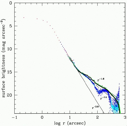
Figure 1: The PSF of the 40-inch Swope telescope at Las Campanas Observatory. The y-axis shows surface brightness scaled to correspond to the total flux of a zero magnitude star. The profile within 5″ was measured from unsaturated stars and can be affected by seeing. The outer profile was measured from two stars with super-saturated cores imaged in two different bands. The profile with the bump in it at 100″ is the $r-$band profile, that without the bump is the $B-$band PSF. The bump in the profile at 100″ is due to a reflection off the CCD which then bounces off of the filter, and back down onto the CCD. The outer surface brightness profile decreases as $r^{-2}$ in the $r-$band and $r^{-1.6}$ in the $B$, shown by the dashed lines. An $r^{-3.9}$ profile is plotted to show the range in slopes.

Scattered light in the telescope and atmosphere produce an extended point spread function (PSF) for all objects. To correct for this effect, we determine the extended PSF using the profiles of a collection of stars from super-saturated 4th mag stars to unsaturated 14th magnitude stars. The radial profiles of these stars were fit together to form one PSF such that the extremely saturated star was used to create the profile at large radii and the unsaturated stars were used for the inner portion of the profile. This allows us to create an accurate PSF to a radius of $7$′, shown in Figure 1.

The inner region of the PSF is well fit by a Moffat function. The outer region is well fit by $r^{-2.0}$ in the $r-$band and $r^{-1.6}$ in the $B-$band. In the $r-$band there is a small additional halo of light at roughly 50 - 100″(200-400pix) around stars imaged on the CCD. The newer, higher quality, anti-reflection coated interference $B-$band filter does not show this halo, which implies that the halo is caused by reflections in the filter. To test the effect of clouds on the shape of the PSF we create a second deep PSF from stars in cluster fields taken under non-photometric conditions. There is a slight shift of flux in the inner 10 arcseconds of the PSF profile, which will have no impact on our ICL measurement.

For each individual, non-saturated star, we subtract a scaled band–specific profile from the frame in addition to masking the inner $30$″ of the profile (the region which follows a Moffat profile). For each individual saturated star, to be as cautious as possible with the PSF wings, we have subtracted a stellar profile given the USNO magnitude of that star, and produced a large mask to cover the inner regions and any bleeding. The mask size is chosen to be twice the radius at which the star goes below 30mag arcsec^-2, and therefore goes well beyond the surface brightness limit at which we measure the ICL. We can afford to be liberal with our saturated star masking since most clusters have very few saturated stars which are not near the center of the cluster where we need the unmasked area to measure any possible ICL.

In the specific case of A3880 there are two saturated stars (9th and 10th $r-$band magnitude) within two arcminutes of the core region of the cluster. If we used the same method of conservatively masking (twice the radius of the 30 mag arcsec^-2 aperture), the entire central region of the image where we expect to find ICL would be lost. We therefore consider a less extreme method of removing the stellar profile by iteratively matching the saturated stars’ profiles with the known PSF shape. We measure the saturated star profiles on an image which has had every object except for those two saturated stars masked, as described in §4.2.2. We can then scale our measured PSF to the star’s profile, at radii where there is expected to be no contamination from the ICL, and the star’s flux is not saturated. Since the two stars are within an arcminute of each other, the scaled profiles of the stars are iteratively subtracted from the masked cluster image until the process converges on solutions for the scaling of each star. We still use a mask for the inner region ($\sim 75\arcsec$) where saturation and seeing effect the profile shape.

4.2.2 Galaxies

We want to remove all the flux in our images associated with galaxies. Although some galaxies might follow deVaucouleurs, Sersic, or exponential profiles, those galaxies which are near the centers of clusters can not be fit with these or other models either because of the overcrowding in the center or because their profiles really are different due to their location in a dense environment. A variety of strategies for modeling galaxies within the centers of clusters were explored in Paper 1 and were found to be inadequate for these purposes. Since we can not fit and subtract the galaxies to remove their light, we instead mask all galaxies in our cluster images.

By masking, we remove from our ICL measurements all pixels above a surface brightness limit which are centered on a galaxy as detected by SExtractor. For paper I, we chose to mask inside of 2 - 2.3 times the radius at which the galaxy light dropped below 26.4 mag arcsec^-2 in $r$, akin to 2-2.3 times a Holmberg radius (Holmberg, 1958). Holmberg radii are typically used to denote the outermost radii of the stellar populations in galaxies.

Galaxy profiles will also have the characteristic underlying shape of the PSF, including the extended halo. However for a 20th magnitude galaxy, the PSF is below 30 mag arcsec^-2by a radius of 10″.

Each of the clusters has a different native surface brightness detection threshold based on the illumination correction and background subtraction, and they are all at different redshifts. However we want to mask galaxies at all redshifts to the same physical surface brightness to allow for a meaningful comparison between clusters at different redshifts. To do this we make a correction for $(1+z)^{4}$ surface brightness dimming and a $k$ correction for each cluster when calculating mask sizes. The masks sizes change by an average of 10% and at most 22% from what they would have been given the native detection threshold. Both the native and corrected surface brightness detection thresholds are listed in Table 2. To test the effect of mask size on the ICL profile and total flux, we also create masks which are $30\%$ larger and $30\%$ smaller in area than the calculated mask size. The flux within the masked areas for these galaxies is on average 25% more than the flux identified by SExtractor as the corrected isophotal magnitude for each object.

5 Results

Here we discuss our methods for measuring both cluster and ICL properties as well as a discussion of each individual cluster in our sample.

5.1 Cluster Properties

Cluster redshift, mass, and velocity dispersion are taken from the literature, where available, as listed in table 1. Additional properties that can be identified in our data, particularly those which may correlate with ICL properties (cluster membership, flux, dynamical state, and global density), are discussed below and also summarized in Table 1.

5.1.1 Cluster Membership & Flux

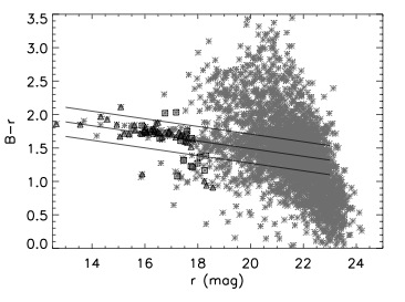
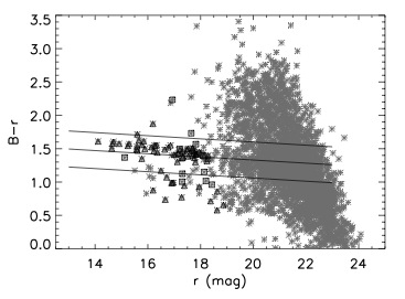
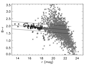
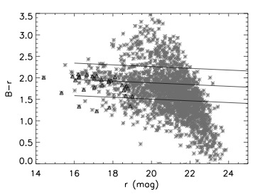
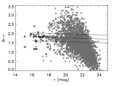
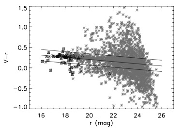
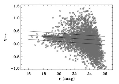
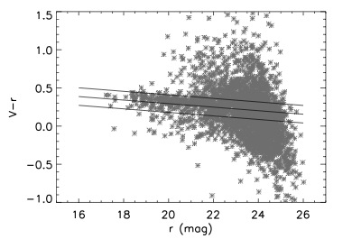
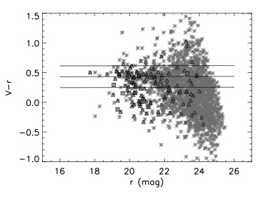
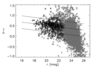
Figure 2: The color magnitude diagrams for all ten clusters in increasing redshift order from let to right, top to bottom; A4059, A3880, A2734, A2556, A4010, A3888, A3984, A014, AC114, AC118. All galaxies detected in our image are denoted with a gray star. Those galaxies which have membership information in the literature are over–plotted with open black triangles (members) or squares (non–members)(membership references are given in §A.1- A.10). Solid lines indicate a biweight fit to the red sequence with $1\sigma$ uncertainties.

Cluster membership and galaxy flux are both determined using a color magnitude diagram (CMD) of either $B-r$ vs. $r$ (clusters with $z<0.1$) or $V-r$ vs. $r$ (clusters with $z>0.1$). We create color magnitude diagrams for all clusters using corrected isophotal magnitudes as determined by SExtractor. Membership is then assigned based on a galaxy’s position in the diagram. If a given galaxy is within $1\sigma$ of the red cluster sequence (RCS) determined with a biweight fit, then it is considered a member (fits are shown in Figure 2). All others are considered to be non-member foreground or background galaxies. This method selects the red elliptical galaxies as members. The benefits of this method are that membership can easily be calculated with 2 band photometry. The drawbacks are that it both does not include some of the bluer true members and does include some of the redder non-members. An alternative method of determining cluster flux without spectroscopy by integrating under a background subtracted luminosity function is discussed in detail in §5.3 of paper I. Due to the large uncertainties involved in both methods ($\sim 30\%$), the choice of procedure will not greatly effect the conclusions.

To determine the total flux in galaxies, we sum the flux of all member galaxies within the same cluster radius. The image size of our low-redshift clusters restricts that radius to one quarter of the virial radius of the cluster where virial radii are taken from the literature or calculated from X–ray temperatures as described in §A.1-A.10. From tests with those clusters where we do have some spectroscopic membership information from the literature (see §A.3 & §A.6), we expect the uncertainty in flux from using the CMD for membership to be $\sim 30\%$.

Fits to the CMDs produce the mean color of the red ellipticals, the slope of the color versus magnitude relation (CMR) for each cluster, and the width of that distribution. Among our 10 clusters, the color of the red sequence is correlated with redshift whereas the slopes of the relations are roughly the same across redshift, consistent with López-Cruz et al. (2004). The widths of the CMRs vary from 0.1 to 0.4 magnitudes. This is expected if these clusters are made up of multiple clumps of galaxies all at similar, but not exactly the same, redshifts. True background and foreground groups and clusters can also add to the width of the RCS.

In order to compare fluxes from all clusters, we consider two correction factors. First, galaxies below the detection threshold will not be counted in the cluster flux as we have measured it, and will instead contribute to the ICL flux. Since each cluster has a different detection threshold based mainly on the quality of the illumination correction (see Table 2), we calculate individually for each cluster the flux contribution from galaxies below the detection threshold. Without luminosity functions for each cluster, we adopt the Goto et al. (2002) luminosity function based on 200 Sloan clusters ($\alpha_{r}^{\prime}=-0.85\pm 0.03$). The flux from dwarf galaxies below the detection threshold ( $M=-11$ in $r$) is less than or equal to 0.1% of the flux from sources above the detection threshold (our assumed value of total flux). This is an extremely small contribution due to the faint end slope, and our deep, uniform images with detection thresholds in all cases more than 7 magnitudes dimmer than $M_{*}$. Our surface brightness detection thresholds are low enough that we don’t expect to miss galaxies of normal surface brightness below our detection threshold at any redshift assuming that all galaxies at all redshifts have similar central surface brightnesses.

Second, we apply k and evolutionary corrections to account for the shifting of the bandpasses through which we are observing, and the evolution of the galaxy spectra due to the range in redshifts we observe. We use Poggianti (1997) for both of these corrections as calculated for simple stellar population of elliptical galaxies in $B$, $V$, and $r$.

5.1.2 Dynamical Age

Dynamical age is an important cluster characteristic for this work as dynamical age is tied to the number of past interactions among the galaxies. We discuss four methods for estimating cluster dynamical age based on optical and X–ray imaging. The first two methods are based on cluster morphology using Bautz Morgan type and an indication of the presence of a cD galaxy. We use morphology as a proxy for dynamical age since clusters with single large elliptical galaxies at their centers (cD) have presumably been through more mergers and interactions than clusters that have multiple clumps of galaxies where none have settled to the center of the potential. Those clusters with more mergers are dynamically older, therefore clusters with cD galaxies should be dynamically older. Specifically Bautz Morgan type is a measure of cluster morphology defined such that type I clusters have cD galaxies, type III clusters do not have cD galaxies, and type II clusters may show cD-like galaxies which are not centrally located. Bautz Morgan type is not reliable as Abell did not have membership information. To this we add our own binary indicator of cluster morphology; clusters which have single galaxy peaks in the centers of their ICL distributions (cD galaxies) versus clusters which have multiple galaxy peaks in the centers of their ICL distributions (no cD).

We have more information about the dynamical age of the cluster beyond just the presence or absence of a cD galaxy, namely the difference in brightness of the brightest cluster galaxy (BCG) relative to the next few brightest galaxies in the cluster (the luminosity gap statistic Milosavljević et al., 2006), which is our third estimate of dynamical age. Clusters with one bright galaxy that is much brighter than any of the other cluster galaxies imply an old dynamic age because it takes time to form that bright galaxy through multiple mergers. Conversely, multiple evenly bright galaxies imply a cluster that is dynamically young. For our sample we measure the magnitude differences between the first (M1) and second (M2) brightest galaxies that are considered members based on color. We run the additional test of comparing M2-M1 with M3-M1, where consistency between these values insures a lack of foreground or background contamination. Values of M3-M1 range from 0.24 to 1.1 magnitudes and are listed in Table 1. This is the most reliable measure of dynamic age available to us in this dataset. In a sample of 12 galaxy groups from N-body hydrodynamical simulations, D’Onghia et al. (2005) find a clear, strong correlation between the luminosity gap statistic and formation time of the group (spearman rank coefficient of 0.91) such that $\delta$mag increases by $0.69\pm 0.41(1\sigma)$ magnitudes for every one billion years of formation. We assume this simulation is also an accurate reflection of the evolution of clusters and therefore that M3-M1 is well correlated with formation time and therefore dynamical age of the clusters.

The fourth method for measuring dynamical state is based on the X–ray observations of the clusters. In a simulation of 9 cluster mergers with mass ratios ranging from 1:1 to 10:1 with a range of orbital properties, Poole et al. (2006) show that clusters are virialized at or shortly after they visually appear relaxed through the absence of structures (clumps, shocks, cavities) or centroid shifts (X–ray peak vs. center of the X–ray gas distribution). We then assume that spherically distributed hot gas as evidenced by the X–ray morphologies of the clusters free from those structures and centroid shifts implies relaxed clusters which are therefore dynamically older clusters that have already been through significant mergers. With enough photons, X–ray spectroscopy can trace the metallicity of different populations to determine progenitor groups or clusters. X–ray observations are summarized in §A.1 - §A.10.

5.1.3 Global Density

Current global cluster density is an important cluster characteristic for this work as density is correlated with the past interaction rate among galaxies. We would like a measure of the number of galaxies in each of the clusters within some well defined radius which encompasses the potentially dynamically active regions of the cluster. Abell chose to calculate global density as the number of galaxies with magnitudes between that of the third ranked member, M3, and M3+2 within 1.5 Mpc of the cluster, statistically correcting for foreground and background galaxy contamination with galaxy densities outside of 1.5Mpc (Abell et al., 1989). The cluster galaxy densities are then binned into richness classes with values of zero to three, where richness three clusters are higher density than richness zero clusters. Cluster richnesses are listed in Table 1.

In addition to richness class we use a measure of global density which has not been binned into coarse values and is not affected by sample completeness. To do this we count the number of member galaxies inside of 0.8 $h_{70}^{-1}$Mpc to the same absolute magnitude limit for all clusters. Membership is assigned to those galaxies within $1\sigma$ of the color magnitude relation (CMR). The density may be affected by the width of the CMR if the CMR has been artificially widened due to foreground and background contamination. We choose a magnitude limit of $M_{r}$ = -18.5 which is deep enough to get many tens of galaxies at all clusters, but is shallow enough that our photometry is still complete. At the most distant clusters (z=0.31), an $M_{r}$ = -18.5 galaxy is a $125\sigma$ detection. The numbers of galaxies in each cluster that meet these criteria range from 62 - 288, and are in good agreement with the broader Abell richness determination. These density estimates are listed in Table 1.

5.2 ICL properties

We detect an ICL component in all ten clusters of our sample. We describe below our methods for measuring the surface brightness profile, color, flux, and substructure in that component.

5.2.1 Surface brightness profile

In eight out of 10 clusters the ICL component is centralized enough to fit with a single set of elliptical isophotes. The exceptions are A0141 and AC118. We use the IRAF routine ellipse to fit isophotes to the diffuse light which gives us a surface brightness profile as a function of semi–major axis. The masked pixels are completely excluded from the fits. There are 3 free parameters in the isophote fitting: center, position angle (PA), and ellipticity. We fix the center and let the PA and ellipticity vary as a function of radius. Average ICL ellipticities range from 0.3 to 0.7 and vary smoothly if at all within each cluster. The PA is notably coincident with that of the cD galaxy where present (discussed in §A.1 - A.10).

We identify the surface brightness profile of the total cluster light (ie., including resolved galaxies) for comparison with the ICL within the same radial extent. To do this, we make a new “cluster” image by masking non-member galaxies as determined from the color magnitude relation (§5.1.1). A surface brightness profile of the cluster light is then measured from this image using the same elliptical isophotes as were used in the ICL profile measurement.

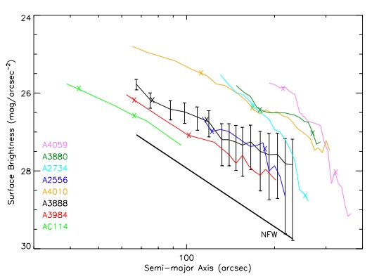
Figure 3: Surface brightness profiles for the eight clusters with a measurable profile. Profiles are listed on the plot in order of ascending redshift. To avoid crowding, error bars are only plotted on one of the profiles. Errors on the other profiles are similar at similar surface brightnesses. All surface brightnesses have been shifted to $z=0$ using surface brightness dimming, k, and evolutionary corrections. The x-axis remains in arcseconds and not in Mpc since the y-axis is in reference to arcseconds. Physical scales are noted on the individual plots (4 - 13). In addition marks have been placed on each profile at the distances corresponding to 200kpc and 300kpc. Also included as the solid black line near the bottom of the plot is a Hubble Reynolds surface brightness profile as a proxy for an NFW density profile with a scale length of 100kpc. The ICL does not have a single uniform amount of flux or profile shape. Profile shape does correlate with dynamical age where those clusters with steeper profiles are dynamically more relaxed (see §6.4).

Figure 3 shows the surface brightness profiles of all eight clusters for which we can measure an ICL profile. Individual ICL profiles in both $r-$ and $V-$ or $B-$bands are shown in Figures 4 - 13. Results based on all three versions of mask size (as discussed in §4.2.2) are shown via shading on those plots. Note that we are not able to directly measure the ICL at small radii ($<\sim 70kpc$) in any of the clusters because greater than 75% of those pixels are masked. The uncertainty in the ICL surface brightness is dominated by the accuracy with which the background level can be identified, while the error on the mean within each elliptical isophote is negligible, as discussed in §5.3. Error bars in Figures 3 and 4 - 13 show the $1\sigma$ uncertainty based on the error budget for each cluster (see representative error budget in Table 3).

The ICL surface brightness profiles have two interesting characteristics. First, in all cases they can be fit by both exponential and deVaucouleurs profiles. Both appear to perform equally well given the large error bars at low surface brightness. These profiles, in contrast to the galaxy profiles, are relatively smooth, only occasionally reflecting the clustering of galaxies. Second, the ICL is more concentrated than the galaxies, which is to say that the ICL falls off more rapidly with increased radius than the galaxy light. In all cases the ICL light is decreasing rapidly enough at large radii such that the additional flux beyond the radius at which we can reliable measure the surface brightness is at most 10% of the flux inside of that radius based on an extrapolation of the exponential fit.

There are 2 clusters (A0141, Figure 11 & AC118, Figure 13) for which there is no single centralized ICL profile. These clusters do not have a cD galaxy, and their giant ellipticals are distant enough from each other that the ICL is not a continuous centralized structure. We therefore have no surface brightness profile for those clusters although we are still able to measure an ICL flux, as discussed below.

We attempt to measure the profile of the cD galaxy where present in our sample. To do this we remove the mask of that galaxy and allow ellipse to fit isophotes all the way into the center. In 5 out of 7 clusters with a cD galaxy, the density of galaxies at the center is so great that just removing the mask for the cD galaxy is not enough to reveal the center of the cluster due to the other overlapping galaxies. Only for A4059 and A2734 are we able to connect the ICL profile to the cD profile at small radii. These are shown in Figures 4 & 6.

In both cases the entire profile of the cD plus ICL is well fit by a single DeVaucouleurs profile, although it can also be fit by 2 DeVaucouleurs profiles. The profiles can not be fit with single exponential functions. We do not see a break between the cD and ICL profiles as seen by Gonzalez et al. (2005). While those authors find that breaks in the extended BCG profile are common in their sample, $\sim 25\%$ of the BCG’s in that sample did not show a clear preference for a double deVaucouleurs model over the single deVaucouleurs model. In both clusters where we measure a cD profile, the color appears to start out with a blue color gradient, and then turn around and become increasingly redder at large radii as the ICL component becomes dominant (see Figures 4 & 6).

5.2.2 ICL Flux

The total amount of light in the ICL and the ratio of ICL flux to total cluster flux can help constrain the importance of galaxy disruption in the evolution of clusters. As some clusters have cD galaxies in the centers of their ICL distribution, we need a consistent, physically motivated method of measuring ICL flux in the centers of those clusters as compared to the clusters without a single centralized galaxy. The key difference here is that in cD clusters the ICL stars will blend smoothly into the galaxy occupying the center of the potential well, whereas with non-cD clusters the ICL stars in the center are unambiguous. Since our physical motivation is to understand galaxy interactions, we consider ICL to be all stars which were at some point stripped from their original host galaxies, regardless of where they are now.

In the case of clusters with cD galaxies, although we cannot separate the ICL from the galaxy flux in the center of the cluster, we can measure the ICL profile outside of the cD galaxy. Gonzalez et al. (2005) have shown for a sample of 24 clusters that a BCG with ICL halo can be well fit with two deVaucouleurs profiles. The two profiles imply two populations of stars which follow different orbits. We assume stars on the inner profile are cD galaxy stars and those stars on the outer profile are ICL stars. Gonzalez et al. (2005) find that the outer profile on average accounts for 80% of the combined flux and becomes dominant at 40-100kpc from the center which is at surface brightness levels of 24 - 25 mag arcsec^-2 in $r$. Since all of our profiles are well beyond this radius and well below this surface brightness level, we conclude that the ICL profile we identify is not contaminated by cD galaxy stars. Assuming that the stars on the outer profile have different orbits than the stars on the inner profile, we calculate ICL flux by summing all the light in the outer profile from a radius of zero to the radius at which the ICL becomes undetectable. Note that this method identifies ICL stars regardless of their current state as bound or unbound from the cD galaxy.

We therefore calculate ICL flux by first finding the mean surface brightness in each elliptical annuli where all masked pixels are not included. This mean flux is then summed over all pixels within that annulus including the ones which were masked. This represents a difference from paper I where we performed an integration on the fit to the ICL profile; here we sum the profile values themselves. We are justified in using the area under the galaxy masks for the ICL sum since the galaxies only account for less than 3% of the volume of the cluster regardless of projected area.

There are two non-cD clusters (A141 & A118) for which we could not recover a profile. We calculate ICL flux for those clusters by measuring a mean flux within three concentric, manually–placed, elliptical annuli (again not utilizing masked pixels) in the mean, and then summing that flux over all pixels in those annuli. All ICL fluxes are subject to the same k and evolutionary corrections as discussed in §5.1.1.

5.2.3 ICL Fraction

In addition to fluxes, we present the ratio of ICL flux to total cluster flux, where total cluster flux includes ICL plus galaxy flux. Galaxy flux is taken from the CMDs out to $0.25r_{virial}$, as discussed in §5.1.1. ICL fractions range from 6 to 22% in the $r-$band and 4 to 21% in the $B-$band where the smallest fraction comes from A2556 and the largest from A4059. All fluxes and fractions are listed in Table 1. As mentioned in §5.1.1, there is no perfect way of measuring cluster flux without a complete spectroscopic survey. Based on those clusters where we do have some spectroscopic information, we estimate the uncertainty in the cluster flux to be $\sim 30\%$ . This includes both the absence from the calculation of true member galaxies, and the false inclusion of non-member galaxies.

All cluster fluxes as measured from the RCS do not include blue member galaxies so those fluxes are potentially lower limits to the true cluster flux, implying that the ICL fractions are potentially biased high. This possible bias is made more complicated by the known fact that not all clusters have the same amount of blue member galaxies (Butcher & Oemler, 1984). Less evolved clusters (at higher redshifts) will have higher fractions of blue galaxies than more evolved clusters (at lower redshifts). Therefore ICL fractions in the higher redshift clusters will be systematically higher than in the lower redshift clusters since their fluxes will be systematically underestimated. We estimate the impact of this effect using blue fractions from Couch et al. (1998) who find maximal blue fractions of $60\%$ of all cluster galaxies at $z=0.3$ as compared to $\sim 20\%$ at the present epoch. If none of those blue galaxies were included in our flux measurement for AC114 and AC118 (the two highest z clusters), this implies a drop in ICL fraction of $\sim 40\%$ as compared to $\sim 10\%$ at the lowest redshifts. This effect will strengthen the relations discussed below.

Most simulations use a theoretically motivated definition of ICL which determine its fractional flux within $r_{200}$ or $r_{vir}$. It is not straightforward to compare our data to those simulated values since our images do not extend to the virial radius nor do they extend to infinitely low surface brightness which keeps us from measuring both galaxy and ICL flux at those large radii. The change in fractional flux from $0.25r_{vir}$ to $r_{vir}$ will be related to the relative slopes of the galaxies versus ICL. As the ICL is more centrally concentrated than the galaxies we expect the fractional flux to decrease from $0.25r_{vir}$ to $r_{vir}$ since the galaxies will contribute an ever larger fraction to the total cluster flux at large radii. We estimate what the fraction at $r_{vir}$ would be for 2 clusters in our sample, A4059 and A3984 (steep profile and shallow profile respectively), by extrapolating the exponential fits to both the ICL and galaxy profiles. Using the extrapolated flux values, the fractional flux decreases by 10% where ICL and galaxy profiles are steep and up to 90% where profiles are shallower.

5.2.4 Color

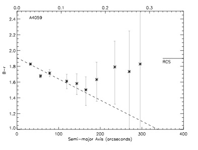
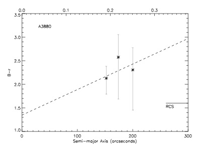
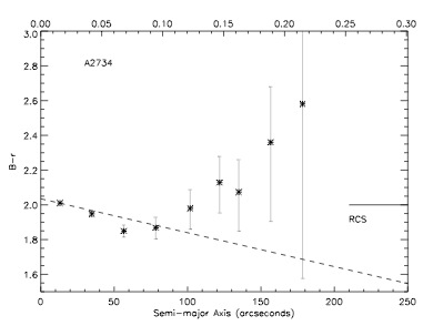
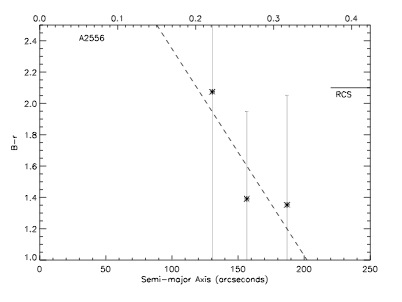
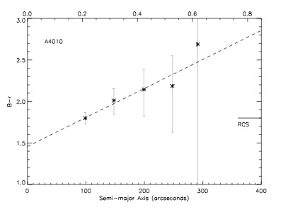
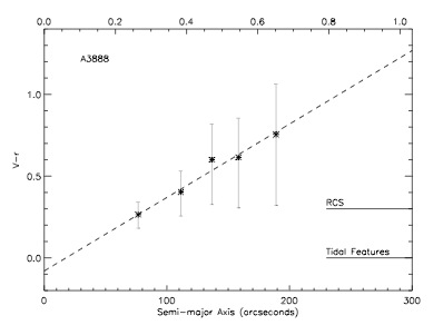
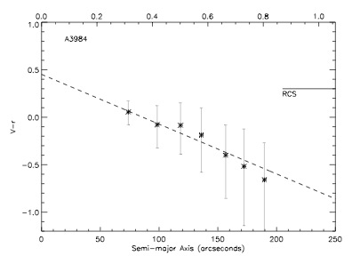
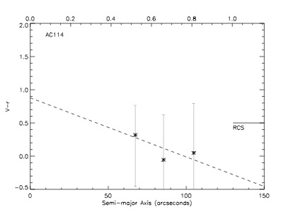
Figure 14: The color profile of the eight clusters where measurement was possible plotted as a function of semi-major axis in arcseconds on the bottom and Mpc on the top. The average color of the red cluster sequence is shown for comparison, as well as the best fit linear function to the data.

For those clusters with an ICL surface brightness profile we measure a color profile as a function of radius by binning together three to four points from the surface brightness profile. All colors are k corrected and evolution corrected assuming a simple stellar population (Poggianti, 1997). Color profiles range from flat to increasingly red or increasingly blue color gradients (see Figures 14). We fit simple linear functions to the color profiles with their corresponding errors. To determine if the color gradients are statistically significant we look at the $\pm 2\sigma$ values on the slope of the linear fit. If those values do not include zero slope, then we assume the color gradient is real. Color error bars are quite large, so in most cases $2\sigma$ does include a flat profile. The significant color gradients (A4010, A3888, A3984) are discussed in §A.1 - A.10.

For all clusters an average ICL color is used to compare with cluster properties. In the case where there is a color gradient, that average color is taken as an average of all points with error bars less than one magnitude.

5.2.5 ICL Substructure

Using the technique of unsharp masking (subtracting a smoothed version of the image from itself) we scan each cluster for low surface brightness (LSB) tidal features as evidence of ongoing galaxy interactions and thus possible ongoing contribution to the ICL . All 10 clusters do have multiple LSB features which are likely from tidal interactions between galaxies, although some are possibly LSB galaxies seen edge on. For example we see multiple interacting galaxies and warped galaxies, as well as one shell galaxy. For further discussion see §6.5 of paper I. From the literature we know that the two highest redshift clusters in the sample (AC114 and AC118, z=0.31) have a higher fraction of interacting galaxies than other clusters ($\sim 12\%$ of galaxies, Couch et al., 1998). In two of our clusters, A3984 and A141, there appears to be plume-like structure in the diffuse ICL, which is to say that the ICL stretches from the BCG towards another set of galaxies. Of this sample, only A3888 has a large, hundred kpc scale, arc type feature, see Figure 9 and Table 2 of paper I. There are $\sim 4$ examples of these large features in the literature (Gregg & West, 1998; Calcáneo-Roldán et al., 2000; Feldmeier et al., 2004; Mihos et al., 2005). These structures are not expected to last longer than a few cluster crossing times, so we don’t expect that they must exist in our sample. Furthermore, it is possible that there is significant ICL substructure below our surface brightness limits (Rudick et al., 2006).

5.2.6 Groups

In seven out of 10 clusters the diffuse ICL is determined by eye to be multi-peaked
(A4059,A2734,A3888,A3984,A141,AC114,AC118). In some cases those excesses surround the clumps of galaxies which appear to all be part of the same cluster, ie the clumps are within a few hundred kpc from the center but have obvious separations, and there is no central dominant galaxy (eg., A118). In other cases, the secondary diffuse components are at least a Mpc from the cluster center (eg., A3888). In these cases, the secondary diffuse light component is likely associated with groups of galaxies which are falling in toward the center of the cluster, and may be at various different stages of merging at the center. This is strong evidence for ICL creation in group environments, which is consistent with recent measurements of a small amount of ICL in isolated galaxy groups (Castro-Rodríguez et al., 2003; Durrell et al., 2004; Rocha & de Oliveira, 2005). This is also consistent with current simulations (Willman et al., 2004; Fujita, 2004; Gnedin, 2003b; Rudick et al., 2006; Sommer-Larsen, 2006, and references therein). From the theory, we expect ICL formation to be linked with the number density of galaxies. Since group environments can have high densities at their centers and have lower velocity dispersions, it is not surprising that groups have ICL flux associated with them. Sommer-Larsen (2006) find the intra-group light to have very similar properties to the ICL making up $12-45\%$ of the group light, having roughly deVaucouleurs profiles, and in general varying in flux from group to group where groups with older dynamic ages (fossil groups D’Onghia et al., 2005) have a larger amount of ICL. Groups in individual clusters are discussed in §A.1 - A.10.

5.3 Accuracy Limits

The accuracy of the ICL surface brightness is limited on small scales ($<10\arcsec$) by photon noise. On larger scales ($>10\arcsec$), structure in the background level (be it intrinsic or instrumental) will dominate the error budget. We determine the stability of the background level in each cluster image on large scales by first median smoothing the masked image by 20″. We then measure the mean flux in thousands of random 1″ regions more distant than 0.8 Mpc from the center of the cluster. The standard deviation of these regions represents the accuracy with which we can measure the background on $20\arcsec$ scales. We tested the accuracy of this measure for even larger-scale uncertainties on two clusters (A3880 from the 40” data and A3888 from the 100” data). We find that the uncertainty remains roughly constant on scales equal to, or larger than, $20\arcsec$. These accuracies are listed for each cluster in Table 2. Regions from all around the frame are used to check that this estimate of standard deviation is universal across the image and not affected by location in the frame. This empirical measurement of the large-scale fluctuations across the image is dominated by the instrumental flat-fielding accuracy, but includes contributions from the bias and dark subtraction, physical variations in the sky level, and the statistical uncertainties mentioned above.

We examine the effect of including data taken under non-photometric conditions on the large-scale background illumination. This noise is fully accounted for in the measurement described above. All $B-$ and $V-$ band data were taken on photometric nights. Five clusters include varying fractions of non-photometric $r-$ band data; $47\%$ of A3880, $12\%$ of A3888, $15\%$ of A3984, $48\%$ of A141, and $14\%$ of A114 are non-photometric. For A3880, the cluster with one of the largest fractions of non-photometric data, we compare the measured accuracy on the combined image which includes the non-photometric data with accuracy measured from a combined image which includes only photometric frames. The resulting large-scale accuracy is 0.3 mag arcsec^-2better on the frame which includes only photometric data. Although this does imply that the non-photometric frames are noisier, the added signal strength gained from having 4.5 more hours on source outweighs the extra noise.

This empirical measurement of the large–scale background fluctuations is likely to be a conservative estimate of the accuracy with which we can measure surface brightness on large scales because it is derived from the outer regions of the image where compared to the central regions on average a factor of $\sim 2$ fewer individual exposures have been combined for the 100” data and a factor of $~{}1.5$ for the 40” (which has a larger field of view and requires less dithering). A larger number of dithered exposures at a range of airmass, lunar phase, photometric conditions, time of year, time of night, and distance to the moon has the effect of smoothing out large-scale fluctuations in the illumination pattern. We therefore expect greater accuracy in the center of the image where the ICL is being measured.

We include a list all sources of uncertainty for one cluster in our sample (A3888) in Table 3 (reproduced here from Paper I). In addition to the dominant uncertainty due to the large-scale fluctuations on the background as discussed above, we quantify the contributions from the photometry, masking, and the accuracy with which we can measure the mean in the individual elliptical isophotes. Errors for the other clusters are similarly dominated by background fluctuations, which are listed in Table 2. The errors on the total ICL fluxes in all bands range from 17% to 70% with an average of 39%. The exception is A2556 which reaches a flux error of 100% in the $B-$band due to its extremely faint profile (see §A.4). Assuming a 30% error in the galaxy flux (see §5.1.1), the errors on the ICL fraction are on average 48%. The errors plotted on the surface brightness profiles are the $1\sigma$ errors.

6 Discussion

We measure a diffuse intracluster component in all ten clusters in our sample. Clues to the physical mechanisms driving galaxy evolution come from comparing ICL properties with cluster properties. We have searched for correlations between the entire set of properties. Pairs of properties not explicitly discussed below showed no correlations. Limited by a small sample and non-parametric data, we use a Spearman rank test to determine the strength of any possible correlations where 1.0 or -1.0 indicate a definite correlation or anti–correlation respectively, and 0 indicates no correlation. Note that this test does not take into account the errors in the parameters, and instead only depends on their rank among the sample. Where a correlation is indicated we show the fit as well as $\pm 2\sigma$ in both y-intercept and slope to graphically show the ranges of the fit, and give some estimate of the strength of the correlation.

There are selection biases in our data between cluster parameters due to our use of an Abell selected sample. The Abell cluster sample is incomplete at high redshifts; it does not include low-mass, low-luminosity, low-density, high-redshift clusters because of the difficulty in obtaining the required sensitivity with increasing redshift. Although our 5 low-redshift clusters are not affected by this selection effect, and should be a random sampling, small numbers prevent those clusters from being fully representative of the entire range of cluster properties.

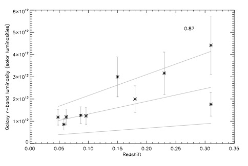
Figure 15: Redshift versus total galaxy flux within one quarter of a virial radius. The Spearman rank coefficient is printed in the upper right corner. The best fit linear function as well as the lines representing $\pm 2\sigma$ in both slope and y intercept are also plotted. The strong correlation between redshift and total galaxy flux shows the incompleteness of the Abell sample which does not include high-redshift, low-flux clusters

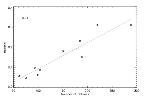
Figure 16: Projected number of galaxies versus redshift. Galaxies brighter than $M_{r}=-18.5$ within 800 $h_{70}^{-1}$kpc are included in this count, which is used as a proxy for density. The Spearman rank coefficient is printed in the upper left corner. There is a strong correlation between density and redshift. The best fit linear function is included. While we do expect clusters to become less dense over time, this strong correlation is not expected. Instead this is due to an incompleteness at high redshift. See §6 for a discussion of the effects of this selection effect.

Specifically we discuss the possibility that there is a real trend underlying the selection bias in the cases of lower luminosity (Figure 15) and lower density clusters (Figure 16) being preferentially found at lower redshift. Clusters in our sample with less total galaxy flux are preferentially found at low redshifts, however hierarchical formation predicts the opposite trend; clusters should be gaining mass over time and hence light over time. Note that on size scales much larger than the virial radius mass does not change with time and therefore those systems can be considered as closed boxes; but on the size scales of our data, a quarter of a virial radius, clusters are not closed boxes.

We might expect a slight trend, as was found, such that lower density clusters are found at lower redshifts. As a cluster ages, it converts a larger number of galaxies into a smaller number of galaxies via merging and therefore has a lower density at lower redshifts despite being more massive than high redshift clusters. The infall of galaxies works against this trend. The sum total of merger and infall rates will control this evolution of density with redshift. The observed density redshift relation for this sample is strong; over the range z=0.3 - 0.05 (elapsed time of 3Gyr assuming standard $\Lambda CDM$) the projected number density of galaxies has to change by a factor of 5.5, implying that every 5.5 galaxies in the cluster must have merged into 1 galaxy in the last 3 Gyr. This is well above a realistic merger rate for this timescale and this time period (Gnedin, 2003a). Instead it is likely that we are seeing the result of a selection effect.

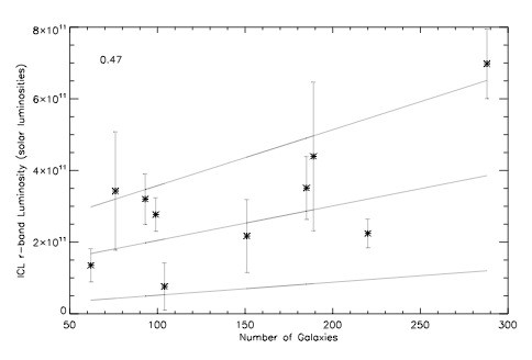
Figure 17: Projected number of galaxies versus ICL luminosity. ICL luminosity shows $1\sigma$ error bars and has been K and evolution corrected. Galaxies brighter than $M_{r}=-18.5$ within 800 $h_{70}^{-1}$kpc are included in this count, which is used as a proxy for density. The Spearman rank coefficient is printed in the upper left corner. The best fit linear function as well as the lines representing $\pm 2\sigma$ in both slope and y intercept are also plotted. There is a mild correlation between density and ICL luminosity such that higher density clusters have a larger amount of ICL flux.

An interesting correlation which may be indirectly due to the selection bias is that clusters with less total galaxy flux tend to have lower densities (Figure 17). While we expect a smaller number of average galaxies to emit a smaller amount of total light, it is possible that the low density clusters are actually made up of a few very bright galaxies. So although the trend might be real, it is also likely that the redshift selection effect of both density and cluster flux is causing these two parameters to be correlated.

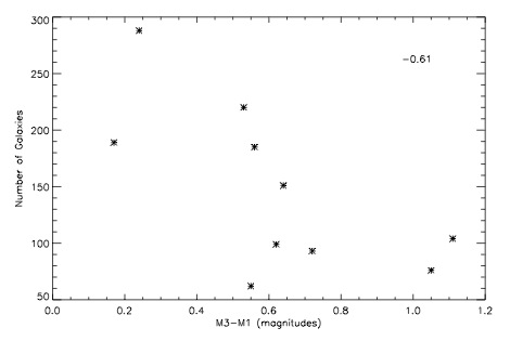
Figure 18: The difference in magnitude between the first and third ranked galaxy versus projected number of galaxies brighter than $M_{r}=-18.5$ within 800 $h_{70}^{-1}$kpc, which is used as a proxy for density. Clusters with cD galaxies will have larger M3-M1 values. This plot implies that over time galaxies merge in clusters to make a cD galaxy, and by the time the cD galaxy has formed, the global density is lower. As discussed in the §6, we assume this is not a selection bias.

A correlation which does not appear to be affected by sample selection is that lower density clusters in our sample are weakly correlated with the presence of a cD galaxy, see Figure 18. A possible explanation for this is that as a cluster ages it will have made a cD galaxy out of many smaller galaxies, so the density will actually be lower for dynamically older clusters. Loh & Strauss (2006) find the same correlation by looking at a sample of environments around 2000 SDSS luminous red galaxies.

In the remainder of this section we examine the interesting physics that can be gleaned from the combination of cluster properties and ICL properties given the above biases. The interpretation of ICL correlations with cluster properties is highly complicated due not only to small number statistics and the selection bias, but to the direction of the selection bias. Biases in mass, density, and total galaxy flux with redshift will destructively combine to cancel the trends which we expect to find in the ICL (as described in the introduction). An added level of complication is due to the fact that we expect the ICL flux to be evolving with time. We examine below each ICL property in turn, including how the selection bias will effect any conclusions drawn from the observed trends.

6.1 ICL flux

We see a range in ICL flux likely caused by the differing interaction rates and therefore differing production of tidal tails, streams, plumes, etc. in different clusters. Clusters include a large amount of tidal features at low surface brightness as evidenced by their discovery at low redshift where they are not as affected by surface brightness dimming (Mihos et al., 2005). It is therefore not surprising that we see a variation of flux levels in our own sample.

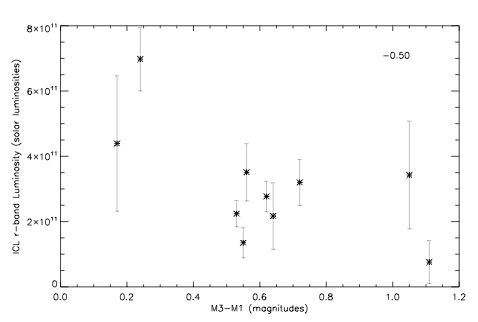
Figure 19: The difference in magnitude between the first and third ranked galaxy versus ICL luminosity. ICL luminosity shows $1\sigma$ error bars and has been K and evolution corrected. Clusters which have cD galaxies have larger M3 - M1 values and are dynamically older clusters. There is a mild correlation between dynamic age and ICL luminosity indicating that the ICL evolves at roughly the same rate as the cluster.

ICL flux is apparently correlated with three cluster parameters; M3-M1, density, and total galaxy flux (Figures 19, 17, & 20). There is no direct, significant correlation between ICL flux and redshift. As discussed above, the selection effects of density and mass with redshift will tend to cancel any expected trends in either density, mass, or redshift. We therefore are unable to draw conclusions from these correlations. Zibetti et al. (2005), who have a sample of 680 SDSS clusters, are able to split their sample on both richness and magnitude of the BCG (as a proxy for mass). They find that both richer clusters and brighter BCG clusters have brighter ICL than poor or faint clusters.

6.1.1 ICL Flux vs. M3-M1

Figure 19 shows the moderate correlation between ICL flux and M3-M1 such that clusters with cD galaxies have less ICL than clusters without cD galaxies (Spearman coefficient of -0.50). Although we choose M3-M1 to be cautious about interlopers, M2-M1 shows the same trend with a slightly more significant spearman coefficient of -0.61. Our simple binary indicator of the presence of a cD galaxy gives the same result. Clusters with cD galaxies (7) have an average flux of $2.3\pm 0.96\times 10^{11}(1\sigma)$ whereas clusters without cD galaxies (3) have an average flux of $5.0\pm 0.18\times 10^{11}(1\sigma)$.

Although density is correlated with M3-M1, and density is affected by incompleteness, this trend of ICL flux with M3-M1 is not necessarily caused by that selection effect. Furthermore, the correlation of M3-M1 with redshift is much weaker (if there at all) than trends of either density or cluster flux with redshift. If the observed relation is due to the selection effect then we are prevented from drawing conclusions from this relation. Otherwise, if this relation between ICL flux and the presence of a cD galaxy is not caused by a selection effect, then we conclude that the lower levels of measured ICL are a result of the ICL stars being indistinguishable form the cD galaxy and therefore the ICL is evolving in a similar way to a cD galaxy.

By which physical mechanism can the ICL stars end up in the center of the cluster and therefore overlap with cD stars? cD galaxies indicate multiple major mergers of galaxies which have lost enough energy or angular momentum to now reside in the center of the cluster potential well. ICL stars on their own will not be able to migrate to the center over any physically reasonable timescales unless they were stripped at the center, or are formed in groups and get pulled into the center along with their original groups(Merritt, 1984).

Assuming the ICL is observationally inseparable from the cD galaxy, we investigate how much ICL light the measured relation implies is hidden amongst the stars of the cD galaxy. If 20% of the total cD + ICL light is added to the value of the ICL flux in the outer profile, then the observed trend of ICL flux with M3-M1 is weakened (Spearman coefficient drops from 0.5 to 0.4). If 30% of the total cD + ICL light is hidden in the inner profile then the relation disappears (Spearman coefficient of 0.22). The measured relation between ICL $r-$band flux and dynamical age of the clusters may then imply that 25-40% of the ICL is coincident with the cD galaxy in dynamically relaxed clusters.

6.2 ICL fraction

We focus now on the fraction of total cluster light which is in the diffuse ICL. If ICL and galaxy flux do scale together (not just due to the selection effect), then the ICL fraction is the physically meaningful parameter in comparison to cluster properties.

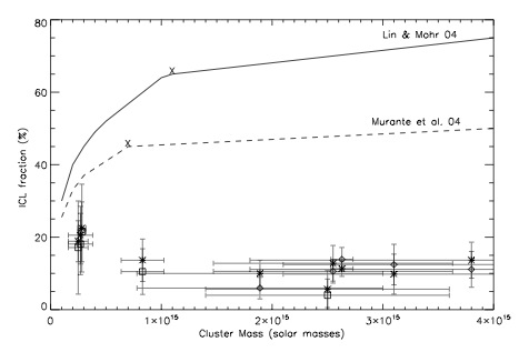
Figure 21: Cluster mass versus the ICL fraction measured at one quarter of the virial radius. Stars denote the $r-$band while squares show $B-$ and diamonds show $V-$band. Errors on ICL fraction are $1\sigma$ as discussed in §5.3. Mass estimates and errors are taken from the literature as discussed in §A.1 - §A.10. The predictions of Lin & Mohr (2004) and Murante et al. (2004) at the virial radius are shown for comparison. These represent extrapolations beyond roughly $1\times 10^{15}$ M_⊙ in both cases (as marked by the crosses). The roughly constant ICL fraction with mass can be explained using hierarchical formation by the in-fall of groups with a similar ICL fraction as the main cluster, or by increased interaction rates with the infall of the groups, or both.

ICL fraction is apparently correlated with both mass and redshift (Figure 21 & 22) and not with density or total galaxy flux. The selection effect will again work against the predicted trend of ICL fraction to increase with increasing mass (Murante et al., 2004; Lin & Mohr, 2004) and increasing density. Therefore the lack of trends of ICL fraction with mass and density could be attributable to the selection bias.

6.2.1 ICL fraction vs. Mass

We find no trend in ICL fraction with mass. Our data for ICL fraction as a function of mass is inconsistent with the theoretical predictions of Murante et al. (2004), Murante et al. (2007) (based on a cosmological hydrodynamical simulation including radiative cooling, star formation, and supernova feedback), and Lin & Mohr (2004)(based on a model of cluster mass and the luminosity of the BCG). However Murante et al. (2007) show a large scatter of ICL fractions within each mass bin. They also discuss the dependence of a simulations mass resolution on the ICL fraction. These theoretical predictions are over-plotted on Figure 21. Note that the simulations generally report the fractional light in the ICL out to much larger radii ($r_{virial}$ or $r_{200}$) than its surface brightness can be measured observationally. To compare the theoretical predictions at $r_{virial}$ to our measurement at $0.25r_{virial}$, the predicted values should be raised by some significant amount which depends on the ICL and galaxy light profiles at large radii. This makes the predictions and the data even more inconsistent than it first appears. As an example of the differences, a cluster with the measured ICL fraction of A3888 would require a factor of greater than 100 lower mass than the literature values to fall along the predicted trend. Although these clusters are not dynamically relaxed, such large errors in mass are not expected. As an upper limit on the ICL flux, if we assumed the entire cD galaxy was made of intracluster stars, that flux plus the measured ICL flux would still not be enough to raise the ICL fractions to the levels predicted by these authors.

There are no evident correlations between velocity dispersion and ICL characteristics, although velocity dispersion is a mass estimator. Large uncertainties are presumably responsible for the lack of correlation.

6.2.2 ICL fraction vs. Redshift

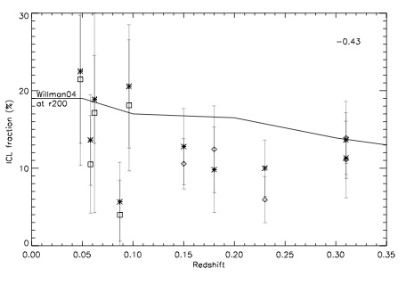
Figure 22: Cluster redshift versus ICL fraction measured at one quarter of the virial radius. As in Figure 21, starred symbols denote the $r-$band, squares show $B-$band, and diamonds show $V-$band fractions. The prediction of Willman et al. (2004) for the ICL fraction as measured at $r_{200}$ is shown for comparison. This prediction would increase if measured at smaller radii, such as was used in our measurement. There is mild evidence for a correlation between redshift and ICL fraction such that ICL fraction grows with decreasing redshift. This trend is consistent with ongoing ICL formation.

Figure 22 is a plot of redshift versus ICL fraction for both the $r-$ and $B-$or $V-$bands. We find a marginal anti–correlation between ICL fraction and redshift with a very shallow slope, if at all, in the direction that low redshift clusters have higher ICL fractions (Spearman rank coefficient of -0.43). This relation is strengthened when assuming fractions of blue galaxies are higher in the higher redshift clusters(spearman rank of -0.6) (see §5.2.3). A trend of ICL fraction with redshift tells us about the timescales of the mechanisms involved in stripping stars from galaxies. This relation is possibly affected by the same redshift selection effects as discussed above.

Over the redshift range of our clusters, $0.31>z>0.05$, a chi–squared fit to our data gives a range of fractional flux of 11 to 14%. Willman et al. (2004) find the ICL fraction grows from 14 to 19%. over that same redshift range. Willman et al. (2004) measure the ICL fraction at $r_{200}$ which means these values would need to be increased in order to directly compare with our values. While their normalization of the relation is not consistent with our data, the slopes are roughly consistent, with the caveat of the selection effect. The discrepancy is likely, at least in part, caused by different definitions of ICL. Simulations tag those particles which become unbound from galaxies whereas in practice we do not have that information and instead use surface brightness cutoffs and ICL profile shapes. Rudick et al. (2006) do use a surface brightness cutoff in their simulations to tag ICL stars which is very similar to our measurement. They find on average from their 3 simulated clusters a change of ICL fraction of approximately 2% over this redshift range. We are not able to observationally measure such a small change in fraction. Rudick et al. (2006) predict that in order to grow the ICL fraction by 10%, on average, we would need to track clusters as they evolve from a redshift of 2 to the present. However, both Willman et al. (2004) and Rudick et al. (2006) find that the ICL fraction makes small changes over short timescales (as major mergers or collisions occur).

6.3 ICL color

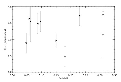
Figure 23: Cluster redshift versus ICL color in $B-r$ which has been k corrected and had simple passive evolution applied to it. If a color gradient is detected in a given cluster then the mean color plotted here is that measured near the center of the profile, weighted slightly toward the center. There is no trend in redshift with ICL color which leads to the conclusion that the ICL is simply passively reddening.

The average color of the ICL, is roughly the same as the color of the red ellipticals in each of the clusters. In §8.1 of paper I we discuss the implications of this on ICL formation redshift and metallicity. Zibetti et al. (2005) have summed $g-$, $r-$, and $i-$ band imaging of 680 clusters in a redshift range of 0.2 - 0.3. Similar to our results, they find that the summed ICL component has roughly the same $g-r$ color at all radii as the summed cluster population including the galaxies. Since we have applied an evolutionary correction to the ICL colors, if there is only passive color evolution, the ICL will show no trend with redshift. Indeed we find no correlation between $B-r$ color and the redshift of the cluster, as shown in Figure 23 ($B-r=2.3\pm 0.2(1\sigma)$). ICL color may have the ability to broadly constrain the epoch at which these stars were stripped. In principle, as mentioned in the introduction, we could learn at which epoch the ICL had been stripped from the galaxies based on its color relative to the galaxies assuming passively evolving ICL and ongoing star formation in galaxies. While this simple theory should be true, the color difference between passively evolving stars and low star forming galaxies may not be large enough to detect since clusters are not made up of galaxies which were all formed at a single epoch and we don’t know the star formation rates of galaxies once they enter a cluster.

ICL color may have the ability to determine the types of galaxies from which the stars are being stripped. Unfortunately the difference in color between stars stripped from ellipticals, and for example stars stripped from low surface brightness dwarfs is not large enough to confirm in our data given the large amount of scatter in the color of the ICL (see paper I for a more complete discussion).

There is no correlation in our sample between the presence or direction of ICL color gradients and any cluster properties. This is very curious since we see both blue-ward and red-ward color gradients. A larger sample with more accurate colors and without a selection bias might be able to determine the origin of the color gradients.

6.4 Profile Shape

Figure 3 shows all eight surface brightness profiles for clusters that have central ICL components. To facilitate comparison, we have shifted all surface brightnesses to a redshift of zero, including a correction for surface brightness dimming, a k–correction, and an evolution correction. We see a range in ICL profile shape from cluster to cluster. This is consistent with the range of scale-lengths found in other surveys (Gonzalez et al., 2005, find a range of scale lengths from 18 - 480 kpc, fairly evenly distributed between 30 and 250 kpc) .

The profiles are equally well fit with the empirically motivated deVaucouleurs profiles and simple exponential profiles which are shown in the individual profile plots in Figures 4 - 13. The profiles can also be fit with a Hubble–Reynolds profile which is a good substitute for the more complicated surface brightness profile of an NFW density profile (Łokas & Mamon, 2001). An example of this profile shape is shown in Figure 3 with a 100 kpc scale length defined as the radius inside of which the profile contains 25% of the luminosity. This profile shape is what you would predict given a simple spherical collapse model. The physically motivated Hubble–Reynolds profile gives acceptable fits to the ICL profiles with the exception of A4059, A2734, & A2556 which have steeper profiles. We explore causes of the differing profile shapes for these three clusters.

A steeper profile is correlated with M3-M1, density, total cluster flux, and redshift. These three clusters have an average M3-M1 value of $0.93\pm 0.27$ as compared to the average of $0.49\pm 0.20$ for the remaining 7 clusters. These three clusters are also three of the four lowest redshift clusters, have an average of 93 galaxies which is 45% smaller than the value for the remaining sample, and have an average cluster flux of $12.3\times 10^{11}$L_⊙which is 47% smaller than the value for the remaining sample.

We have the same difficulties here in distinguishing between the selection effects and the true physical correlations. The key difference is that the three clusters with the steepest profiles are the most relaxed clusters (which is not a redshift selection effect). We use “most relaxed” to describe the three clusters with the most symmetric X–ray isophotes that have single, central, smooth ICL profiles. This is consistent with our finding that M3-M1 is a key indicator of ICL flux in §6.1.1 and that ICL can form either in groups at early times or at later times through galaxy interactions in the dense part of the cluster. If galaxy groups in which the ICL formed are able to get to the cluster center then their ICL will also be found in the cluster center, and can be hiding in the cD galaxy. If the galaxy groups in which the ICL formed have not coalesced in the center then the ICL will be less centrally distributed and therefore have a shallower profile. This is consistent with the recent numerical work by Murante et al. (2007) who find that the majority of the ICL is formed by the merging processes which create the BCG’s in clusters. This process leads o the ICL having a steeper profile shape than the galaxies and having greater than half of the ICL be located inside of $250$$h_{70}^{-1}$kpc, approaching radii where we do not measure the ICL due to the presence of the BCG. Their simulations also confirm that different clusters with different dynamical histories will have differing amounts and locations of ICL.

7 Conclusion

We have identified an intracluster light component in all 10 clusters which has fluxes ranging from $0.76\times 10^{11}$ to $7.0\times 10^{11}$ $h_{70}^{-1}$L_⊙in $r$ and $0.14\times 10^{11}$ to $1.2\times 10^{11}$ $h_{70}^{-1}$L_⊙in the $B-$band, ICL fractions of 6 to 22% of the total cluster light within one quarter of the virial radius in $r$ and 4 to 21% in the $B-$band, and $B-r$ colors ranging from 1.49 to 2.75 magnitudes. This work shows that there is detectable ICL in clusters and groups out to redshifts of at least 0.3, and in two bands including the shorter wavelength $B-$ or $V-$band.

The interpretation of our results is complicated by small number statistics, redshift selection effects of Abell clusters, and the fact that the ICL is evolving with time. Of the cluster properties (M3-M1, density, redshift, and cluster flux), only M3-M1 and redshift are not correlated. As a result of these selection effects ICL flux is apparently correlated with density and total galaxy flux but not with redshift or mass and ICL fraction is apparently correlated with redshift but not with M3-M1, density, total galaxy flux, or mass. However, we do draw conclusions from the ICL color, average values of the ICL fractions, the relation between ICL flux and M3-M1, and the ICL profile shape.

We find a passively evolving ICL color which is similar to the color of the RCS at the redshift of each cluster. The relations between ICL fraction with redshift and ICL fraction with mass show the disagreement of our data with simulations since our fractional fluxes are lower than those predictions. These discrepancies do not seem to be caused by the details of our measurement.

Furthermore we find evidence that clusters with symmetric X–ray profiles and cD galaxies have both less ICL flux and significantly steeper profiles. The lower amount of flux can be explained if ICL stars have become indistinguishable from cD stars. As the cluster formed a cD galaxy any groups which participated in the merging brought their ICL stars with them, as well as created more ICL through interactions. If a cD does not form, then the ICL already in groups or actively forming is also prevented from becoming very centralized as it has no way of loosing energy or angular momentum on its own. While the galaxies or groups are subject to tidal forces and dynamical friction, the ICL, once stripped, will not be able to loose energy and/or angular momentum to these forces, and instead will stay on the orbit on which it formed.

Observed density may not be a good predictor of ICL properties since it does not directly indicate the density at the time in which the ICL was formed. We do indeed expect density at any one epoch to be linked to ICL production at that epoch through the interaction rates.

The picture that is emerging from this work is that ICL is ubiquitous, not only in cD clusters, but in all clusters, and in group environments. The amount of light in the ICL is dependent upon cluster morphology. ICL forms from ongoing processes including galaxy–galaxy interactions and tidal interactions with the cluster potential (Moore et al., 1996; Gnedin, 2003b) as well as in groups (Rudick et al., 2006). With time, as multiple interactions and dissipation of angular momentum and energy lead groups already containing ICL to the center of the cluster, the ICL moves with the galaxies to the center and becomes indistinguishable from the cD’s stellar population. Any ICL forming from galaxy interactions stays on the orbit where it was formed.

A large, complete sample of clusters, including a proportionate amount with high redshift and low density, will be able to break the degeneracies present in this work. Shifting to a lower redshift range will not be as beneficial because a shorter range than presented here will not be large enough to see the predicted evolution in the ICL fraction.

In addition to large numbers of clusters it would be beneficial to go to extremely low surface brightness levels ($<\sim 30$ mag arcsec^-2) to reduce significantly the error bars on the color measurement and thereby learn about the progenitor galaxies of the ICL and the timescales for stripping. It will not be easy to achieve these surface brightness limits for a large sample which includes high-redshift low-density clusters since those clusters will have very dim ICL due to both an expected lower amount as correlated with density, and due to surface brightness dimming.

Table 1: Cluster characteristics

Cluster	$z$	$M_{3}-M_{1}$	Richness	ngals	$\sigma_{v}$	$r_{virial}$	Mass	Cluster Flux		ICL Flux		Ratio		ICL
name		mag	Class		km/s	Mpc	$10^{14}$ M⊙	B $10^{11}$ L⊙	r $10^{11}$ L⊙	B $10^{11}$ L⊙	r $10^{11}$ L⊙	B%	r%	color
A4059†	0.048r	$1.05\pm.05$	1	76	845${}^{\rm+280}_{\rm-140}$t	2.6i	2.82 ${}^{\rm+0.37}_{\rm-0.34}$i	$4.2\pm 1.3$	$12\pm 3.5$	$1.2\pm.24$	$3.4\pm 1.7$	$21\pm 8$	$22\pm 12$	1.89
A3880†	0.058r	$0.55\pm.05$	0	62	827${}^{\rm+120}_{\rm-79}$m	2.5e	8.3 ${}^{\rm+2.8}_{\rm-2.1}$f	$3.8\pm 1.1$	$8.6\pm 2.6$	$0.44\pm 0.23$	$1.4\pm 0.46$	$10\pm 6$	$14\pm 6$	2.63
A2734†	0.062r	$0.62\pm.05$	1	99	628${}^{\rm+61}_{\rm-57}$m	2.4i	2.49 ${}^{\rm+0.89}_{\rm-0.63}$i	$3.4\pm 1.0$	$12\pm 3.6$	$0.7\pm 0.47$	$2.8\pm 0.47$	$17\pm 13$	$19\pm 6$	2.54
A2556†	0.087r	$1.11\pm.05$	1	104	1247${}^{\rm+249}_{\rm-249}$t	2.6e	$25\pm 1$g	$3.3\pm 0.99$	$13\pm 3.8$	$0.14\pm 0.14$	$0.76\pm 0.66$	$4\pm 4$	$6\pm 5$	2.48
A4010†	0.096r	$0.72\pm.05$	1	93	625${}^{\rm+127}_{\rm-95}$m	3.1e	3.8 ${}^{\rm+1.6}_{\rm-1.2}$f	$3.5\pm 1.0$	$12\pm 3.7$	$0.77\pm 0.28$	$3.2\pm 0.70$	$18\pm 8$	$21\pm 8$	2.54
A3888	0.151r	$0.17\pm.04$	2	189	1102${}^{\rm+137}_{\rm-107}$n	3.7i	25.5 ${}^{\rm+10.5}_{\rm-7.4}$i	$7.2\pm 2.2$	$30\pm 9.0$	$0.86\pm.25$	$4.4\pm 2.1$	$11\pm 3$	$13\pm 5$	1.97
A3984†	0.181r	$0.64\pm.04$	2	151	$\cdots$	3.5e	$31\pm 10$c	$4.4\pm 1.3$	$20\pm 6.0$	$0.62\pm 0.21$	$2.2\pm 1.0$	$12\pm 6$	$10\pm 6$	1.49
A0141†	0.23r	$0.56\pm.04$	3	185	$\cdots$	3.7e	18.9 ${}^{\rm+11.1}_{\rm-8.7}$d	$5.4\pm 1.6$	$32\pm 9.5$	$0.34\pm 0.11$	$3.5\pm 0.88$	$6\pm 3$	$10\pm 4$	2.72
AC114	0.31a	$0.45\pm.04$	2	220	1388${}^{\rm+128}_{\rm-71}$n	3.5b	26.3${}^{\rm+8.2}_{\rm-7.1}$n	$2.3\pm 0.70$	$18\pm 5.3$	$0.38\pm 0.08$	$2.2\pm 0.4$	$14\pm 3$	$11\pm 2$	2.15
AC118	0.308r	$0.24\pm.04$	3	288	1947${}^{\rm+292}_{\rm-201}$h	3.4b	$38\pm 37$n	$5.4\pm 1.6$	$44\pm 1.3$	$0.67\pm 0.17$	$7.0\pm 0.97$	$11\pm 5$	$14\pm 5$	2.75

Notes: Sources for the virial radii and mass are discussed in §A.1-A.10 and generally come from X–ray data. ${\dagger}$: We have obtained additional photometric and spectroscopic data for these cluster to be published in a forthcoming paper) a: Abell et al. (1989). b: Allen (1998). c: Cypriano et al. (2004). d: Dahle et al. (2002). e: Ebeling et al. (1996). f: Girardi et al. (1998b). g:Reimers et al. (1996). h: Couch & Sharples (1987). i: Reiprich & Böhringer (2002). m: Girardi et al. (1998a). n: Girardi & Mezzetti (2001). r: Struble & Rood (1999). t: Wu et al. (1999).

Table 2: Observational Parameters

Cluster	redshift	exposure time	average seeing	field of view	native det. tresh.	corrected det. thresh	back. accuracy
		r, B/V hrs	r,B/V arcsecs	$h_{70}^{-1}$Mpc	r,B/Vmag arcsec-2	r,B/Vmag arcsec-2	r,B/Vmag arcsec-2
A4059	0.048	3.8,4.3	1.1,1.7	$1.2\times 1.4$	24.9,25.8	26.25,26.04	27.7,29.9
A3880	0.058	9.5,4.3	1.5,1.5	$1.7\times 2.2$	25.1,25.2	26.22,26.04	28.0,29.2
A2734	0.062	4.6,4.1	1.3,1.7	$1.7\times 1.9$	24.8,25.2	26.21,26.05	28.7,29.3
A2556	0.087	3.8,3.7	1.3,1.4	$2.0\times 2.4$	24.7,25.4	26.13,26.11	27.7,29.4
A4010	0.096	5.5,6.9	1.7,1.3	$2.3\times 2.5$	25.0,25.7	26.10,26.09	28.4,29.9
A3888	0.151	6.3,4.0	1.1,0.9	$2.3\times 2.2$	26.4,26.0	25.94,25.67	28.8,29.5
A3984	0.181	6.8,4.3	1.0,1.0	$2.3\times 2.5$	26.4,25.9	25.89,25.65	28.9,29.0
A0141	0.23	6.8,4.0	0.9,1.0	$2.8\times 2.7$	26.3,26.0	25.75,25.63	29.2,29.8
AC118	0.31	6.0,3.0	1.4,1.0	$2.7\times 2.9$	26.3,26.9	25.62,25.70	29.7,29.9
AC114	0.31	5.5,4.3	1.1,1.8	$2.4\times 2.5$	26.4,26.1	25.63,25.70	29.8,29.8

Note. — The first five clusters in the table were imaged with the 1m Swope telescope in the $r-$ and $B-$bands. The five clusters under the middle line were imaged with the 2.5m DuPont telescope in the $r-$ and $V-$bands. Native detection threshold refers to the measured detection threshold of the cluster at its appropriate redshift. Corrected surface brightness detection threshold refers to the actual detection threshold to which we mask at the redshift of each cluster. This detection threshold has been surface brightness dimming and k-corrected to a redshift of zero, as discussed in §4.2.2.

Table 3: Error Budget

Source			contribution to ICL uncertainty (%)
	$1\sigma$ uncertainty		$\mu$(0″- 100″)		$\mu$(100″- 200″)		total ICL flux
	($V$)	($r$)	($V$)	($r$)	($V$)	($r$)	($V$)	($r$)
background levela	29.5 mag arcsec-2	28.8 mag arcsec-2	14	18	39	45	24	31
photometry	0.02 mag	0.03 mag	2	3	2	3	2	3
maskingb	variation in mask area $\pm 30$		5	5	14	19	9	12
std. dev. in meanc	32.7 mag arcsec-2	32.7 mag arcsec-2	3	2	2	1	3	1
(total)			15	19	41	50	26	33
cluster fluxd	16%	16%	$\cdots$	$\cdots$	$\cdots$	$\cdots$	$\cdots$	$\cdots$

Note. — a: Large scale fluctuations in background level are measured empirically and include instrumental calibration uncertainties as well as and true variations in background level (see §5.3). b: Object masks were scaled by $\pm 30\%$ in area to test the impact on ICL measurement (see §4.2.2). c: The statistical uncertainty in the mean surface brightness of the ICL in each isophote. d: Errors on the total cluster flux are based on errors in the fit to the luminosity function (see §5.1.1).

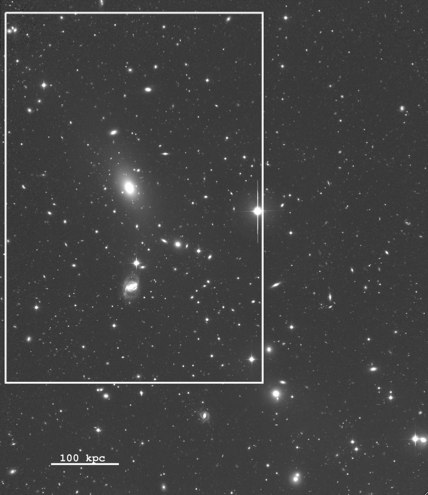
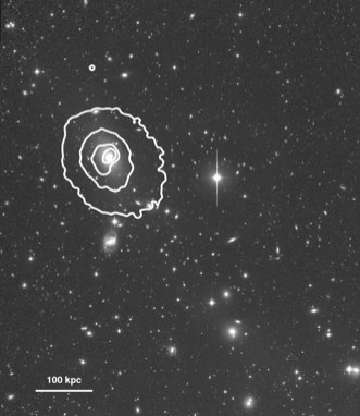
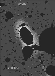
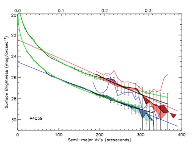
Figure 4: A4059. The plots moving left to right and top to bottom are as follows. The first is our final combined $r-$band image zoomed in on the central cluster region. The second plot shows X–ray isophotes where available. Some clusters were observed during the ROSAT all sky survey, and so have X–ray luminosities, but have not had targeted observations to allow isophote fitting. Isophote levels are derived from quick-look images taken from HEASARC. X-ray luminosities of these clusters are listed in Table 1 of paper I and are discussed in the appendix. The third plot shows our background subtracted, fully masked $r-$band image of the central region of the cluster, smoothed to aid in visual identification of the surface brightness levels. Masks are shown in their intermediate levels which are listed in column 7 of Table 2. The six gray-scale levels show surface brightness levels of up to 28.5, 27.7,27.2,26.7 mag arcsec^-2. The fourth plot shows the surface brightness profiles of the ICL (surrounded by shading;$r-$band on top, $V-$ or $B-$band on the bottom) and cluster galaxies as a function of semi-major axis. The bottom axis is in arcseconds and the top axis corresponds to physical scale in Mpc. Error bars represent the $1\sigma$ background identification errors as discussed in §5.3. DeVaucouleurs fits to the entire cD plus ICL profile are over-plotted.

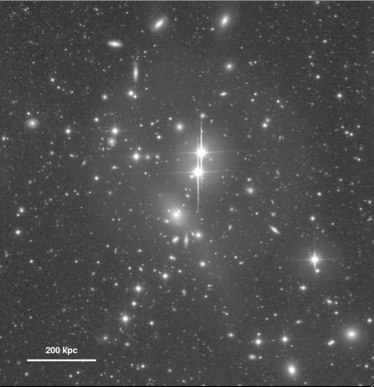
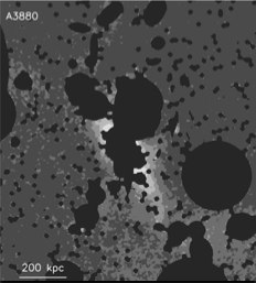
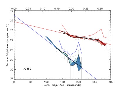
Figure 5: A3880, same as Figure 4

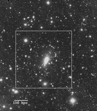
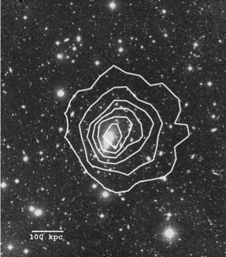
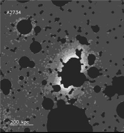
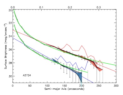
Figure 6: A2734, same as Figure 4

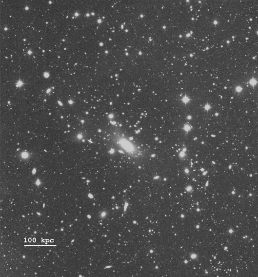
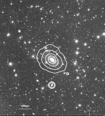
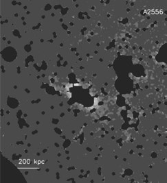
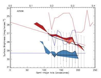
Figure 7: A2556, same as Figure 4

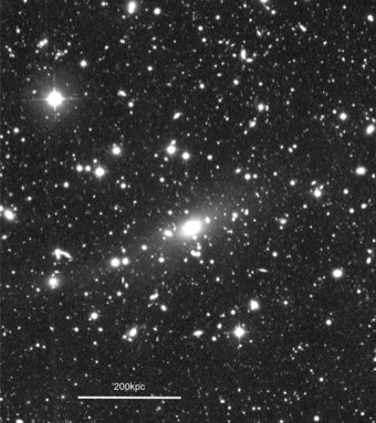
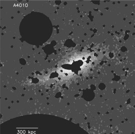
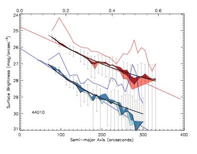
Figure 8: A4010, same as Figure 4

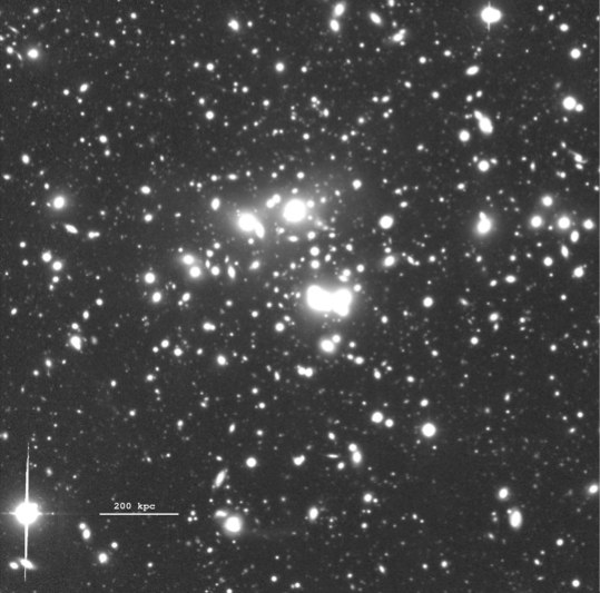
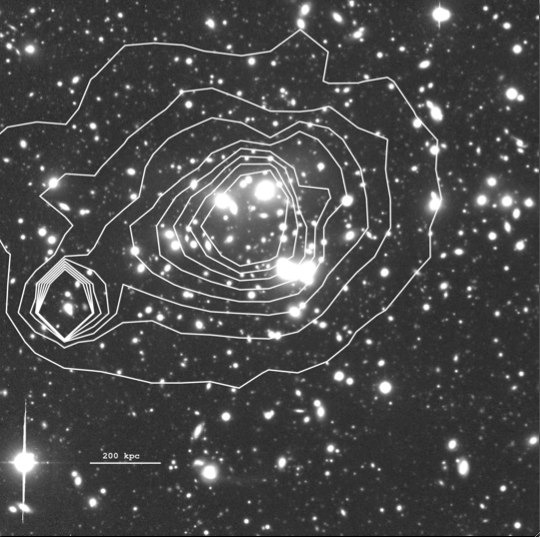
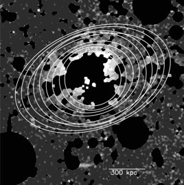
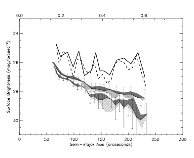
Figure 9: A3888, same as Figure 4, except here we show the elliptical isophotes of the ICL over-plotted on the surface brightness image.

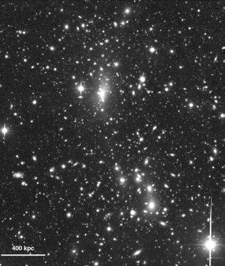
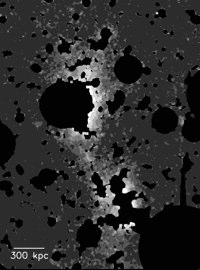
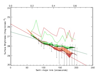
Figure 10: A3984, same as Figure 4

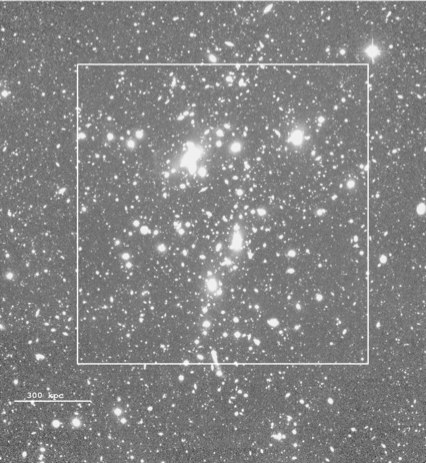
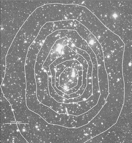
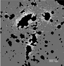
Figure 11: A141, same as Figure 4, except we are not able to measure a surface brightness profile or consequently a color profile.

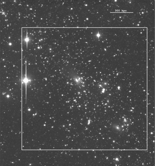
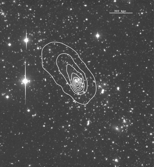
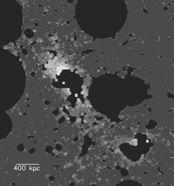
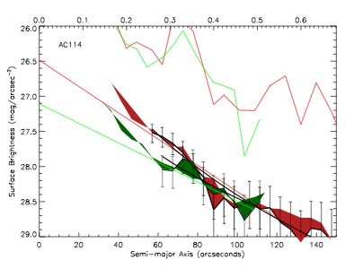
Figure 12: A114, same as Figure 4

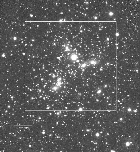
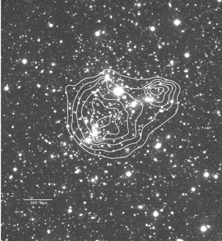
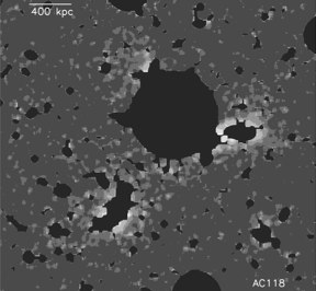
Figure 13: A118, same as Figure 4, except we are not able to measure a surface brightness profile or consequently a color profile.

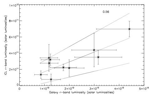
Figure 20: The flux in galaxies versus the flux in ICL in units of solar luminosities. Errors on ICL luminosity are $1\sigma$. Errors on galaxy luminosity are 30% as estimated in §5.1.1. Over-plotted is the best fit linear function as well as two lines which represent $2\sigma$ errors in both y-intercept and slope. The Spearman rank coefficient is printed in the upper right. Here galaxy luminosity is assumed to be a proxy for mass, so we find a significant correlation between mass and ICL flux such that more massive clusters have a larger amount of ICL flux.

Appendix A The Clusters

In order of increasing redshift we discuss interesting characteristics of the clusters and their ICL components. Relevant papers are listed in Table 1. Relevant figures are 4 - 13.

A.1 A4059

A4059 is a richness class 1, Bautz Morgan type I cluster at a redshift of 0.048. There is a clear cD galaxy which is however offset from the Abell center, likely due to the presence of at least two other bright elliptical galaxies. The cD galaxy is $0.91\pm.05$ magnitudes brighter than the second ranked cluster galaxy. The cD galaxy is at the center of the Chandra and ASCA mass distributions. Those telescopes detect no hot gas around the other bright ellipticals. This cluster shows interesting features in it’s X–ray morphology. There appear to be large bubbles, or cavities in the hot gas, which is likely evidence of past radio galaxy interactions with the ICM (Choi et al., 2004). As additional evidence of past activity in this cluster, the cD galaxy contains a large dust lane (Choi et al., 2004). $M_{500}$ (the mass within the radius where the mean mass density is equal to 500 times the critical density) is calculated by Reiprich & Böhringer (2002) for A4059 to be $2.82\pm_{0.34}^{0.37}\times 10^{14}h_{70}^{-1}$ M_⊙.

The color magnitude diagram shows a very tight red sequence. Membership information is taken from Collins et al. (1995), Colless et al. (2001), and Smith et al. (2004). Using the CMD as an indication of membership, we estimate the flux in cluster galaxies to be $1.2\pm.35\times 10^{12}$L_⊙in $r$ and $4.2\pm 1.3\times 10^{11}$L_⊙in $B$ inside of 0.65$h_{70}^{-1}$Mpc, which is one quarter of the virial radius of this cluster. In this particular cluster, since the Abell center is not at the true cluster center, and it is the nearest cluster in our sample, our image does not uniformly cover the entire one quarter of the virial radius. This estimate is therefore below the true flux in galaxies because we are missing area on the cluster.

Figure 4 shows the relevant plots for this cluster. There is a strong ICL component ranging from 26 - 29 mag arcsec^-2 in $r$ centered on the cD galaxy. The total flux in the ICL is $3.4\pm 1.7\times 10^{11}$L_⊙in $r$ and $1.2\pm.24\times 10^{11}$L_⊙in $B$, which makes for ICL fractions of $22\pm 12\%$ in $r$ and $21\pm 8\%$ in $B$. The ICL has a flat color profile with $B-r\simeq 1.7\pm.08$, which is marginally bluer (0.2 magnitudes) than the RCS. One of the two other bright ellipticals at 0.7$h_{70}^{-1}$Mpc from the center has a diffuse component, the other bright elliptical is too close to a saturated star to detect a diffuse component.

A.2 A3880

A3880 is a richness class 0, Bautz Morgan type II cluster at a redshift of 0.058. There is a clear cD galaxy in the center of this cluster, which is $0.52\pm.05$ magnitudes brighter than the second ranked galaxy. This cluster is detected in the ROSAT All Sky Survey, however that survey is not deep enough to show us the shape of the mass distribution. Girardi et al. (1998b) find a mass for this cluster based on its velocity dispersion of $8.3_{-2.1}^{+2.8}\times 10^{14}h_{70}^{-1}\hbox{M${}_{\odot}$}$.

The color magnitude diagram shows a clear red sequence. There is possibly another red sequence at lower redshift adding to the width of the red sequence. Membership information is provided by Collins et al. (1995), Colless et al. (2001), and Smith et al. (2004). Using the CMD as an indication of membership, we estimate the flux in cluster galaxies to be $8.6\pm 2.6\times 10^{11}$L_⊙in $r$ and $3.8\pm 1.1\times 10^{11}$L_⊙in $B$ inside of 0.62$h_{70}^{-1}$Mpc, which is one quarter of the virial radius of this cluster.

Figure 5 shows the relevant plots for this cluster. Unfortunately this cluster has larger illumination problems than the other clusters which can be seen in the greyscale masked image. Nonetheless, there is clearly an $r-$band ICL component, although the $B-$band ICL is extremely faint. The total flux in the ICL is $1.4\pm 2.3\times 10^{11}$L_⊙in $r$ and $4.4\pm 1.5\times 10^{10}$L_⊙in $B$, which makes for ICL fractions of $14\pm 6\%$ in $r$ and $10\pm 6\%$ in $B$. The ICL has a flat color profile with $B-r\simeq 2.4\pm 1.1$, which is 0.8 magnitudes redder than the RCS.

A.3 A2734

A2734 is a richness class 1, Bautz Morgan type III cluster at a redshift of 0.062. The BCG by $0.51\pm.05$ magnitudes is in the center of this cluster, however there are 2 other large elliptical galaxies 0.55$h_{70}^{-1}$Mpc and 0.85$h_{70}^{-1}$Mpc distant from the BCG. The X–ray gas does confirm the BCG as being at the center of the mass distribution. Those 2 other elliptical galaxies are not seen in the 44ks ASCA GIS observation of this cluster, however they are confirmed members based on spectroscopy (Collins et al., 1995; Colless et al., 2001; Smith et al., 2004). $M_{500}$ is calculated by Reiprich & Böhringer (2002) for A2734 to be $2.49\pm_{0.63}^{0.89}\times 10^{14}h_{70}^{-1}$ M_⊙.

The color magnitude diagram shows a clear red sequence, which includes the 3 bright elliptical galaxies. 2df spectroscopy gives us roughly 80 galaxies in our field of view which we can use to estimate the effectiveness of the biweight fit to the RCS in finding true cluster members. Of those galaxies with confirmed membership, 94% are determined members with this method, however 86% of the confirmed non-members are also considered members. This is likely due to how galaxies were selected for spectroscopy in the 2df catalog. Using the CMD as an indication of membership, we estimate the flux in cluster galaxies to be $1.2\pm.36\times 10^{12}$L_⊙in $r$ and $3.4\pm 1.0\times 10^{11}$L_⊙in $B$ inside of 0.60$h_{70}^{-1}$Mpc, which is one quarter of the virial radius of this cluster.

Figure 6 shows the relevant plots for this cluster. There is a strong ICL component ranging from 26 - 29 mag arcsec^-2 in $r$ centered on the BCG. The total flux in the ICL is $2.8\pm.47\times 10^{11}$L_⊙in $r$ and $7.0\pm 4.7\times 10^{10}$L_⊙in $B$, which makes for ICL fractions of $19\pm 6\%$ in $r$ and $17\pm 13\%$ in $B$. The ICL has a flat to red-ward color profile with $B-r\simeq 2.3\pm.03$, which is marginally redder than the RCS (0.3 magnitudes). The cluster has a second diffuse light component around one of the giant elliptical galaxies, .55 $h_{70}^{-1}$Mpc from the center of the cD galaxy. The third bright elliptical has a saturated star just 40″away, so we do not have a diffuse light map of that galaxy.

A.4 A2556

A2556 is a richness class 1, Bautz Morgan type II-III cluster at a redshift of 0.087. Despite the Bautz Morgan classification, this cluster has a clear cD galaxy in the center of the X–ray distribution which is $0.93\pm.05$ magnitudes brighter than any other galaxy in the cluster. The Chandra derived X–ray distribution is slightly elongated toward the NE where a second cluster, A2554, resides, 1.4$h_{70}^{-1}$Mpc from the center of A2556. The cD galaxy of A2554 is just on the edge of our images so we have no information about its low surface brightness component. A2556 and A2554 are a part of the Aquarius supercluster(Batuski et al., 1999), so they clearly reside in an overdense region of the universe. Given an X–ray luminosity from Ebeling et al. (1996) and a velocity dispersion from Reimers et al. (1996), we calculate the virial mass of A2556 to be $2.5\pm 1.1\times 10^{15}h_{70}^{-1}\hbox{M${}_{\odot}$}$.

The red sequence for this cluster is a bit wider than in other clusters. The one sigma width to a biweight fit is 0.38 magnitudes in B-r which is approximately 30% larger than in the rest of the low-z sample. This extra width is not caused by only a few galaxies, instead the entire red sequence appears to be inflated. This is probably caused by the nearby A2554 which is at z=0.11 (Struble & Rood, 1999). This is close enough in redshift space that we cannot separate out the 2 red sequences in our CMD. We have roughly 30 redshifts for A2556 from Smith et al. (2004), Caretta et al. (2004), and Batuski et al. (1999) which are also unable to differentiate between the clusters. Using the CMD as an indication of membership, we estimate the flux in cluster galaxies to be $1.3\pm.38\times 10^{12}$L_⊙in $r$ and $3.3\pm 1.0\times 10^{11}$L_⊙in $B$ inside of 0.65$h_{70}^{-1}$Mpc, which is one quarter of the virial radius of this cluster.

Figure 7 shows the relevant plots for this cluster. There is an $r-$band ICL component ranging from 27 - 29 mag arcsec^-2 in $r$ centered on the cD galaxy. The $B-$band ICL is extremely faint, barely above or detection threshold. Although we were able to fit a profile to the $B-$band diffuse light, all points on the medium sized mask are below 29 mag arcsec^-2. The total flux in the ICL is $7.6\pm 6.6\times 10^{10}$L_⊙in $r$ and $1.4\pm 1.4\times 10^{10}$L_⊙in $B$, which makes for ICL fractions of $6\pm 5\%$ in $r$ and $4\pm 4\%$ in $B$. Although Figure 7 shows a color profile, we do not assume anything about the profile shape due to the low SB level of the $B-$band. We take the $B-r$ color from the innermost point to be $2.1\pm 0.4$, which is fully consistent with the color of the RCS.

A.5 A4010

A4010 is a richness class 1, Bautz Morgan type I-II cluster at a redshift of 0.096. This cluster has a cD galaxy in the center of the galaxy distribution, which is $0.7\pm.05$ magnitudes brighter than the second ranked galaxy. There is only ROSAT All Sky Survey data for this cluster and no other sufficiently deep X–ray observations to show us the shape of the mass distribution. There are weak lensing maps which put the center of mass of the cluster at the same position as the cD galaxy, and elongated along the same position angle as the cD galaxy (Cypriano et al., 2004). Muriel et al. (2002) find a velocity dispersion of $743\pm 140$ for this cluster which is $15\%$ larger than found by Girardi et al. (1998b), where those authors find a virial mass of $3.8\pm_{1.2}^{1.6}\times 10^{14}h_{70}^{-1}$ M_⊙.

The color magnitude diagram for A4010 is typical among the sample with a clear red sequence. A few redshifts exist in the literature which help define the red sequence (Collins et al., 1995; Katgert et al., 1998). Using the CMD as an indication of membership, we estimate the flux in cluster galaxies to be $1.2\pm.4\times 10^{12}$L_⊙in $r$ and $3.5\pm 1.0\times 10^{11}$L_⊙in $B$ inside of 0.75$h_{70}^{-1}$Mpc, which is one quarter of the virial radius of this cluster.

Figure 8 shows the relevant plots for this cluster. There is an elongated ICL component ranging from 25.5 - 28 mag arcsec^-2 in $r$ centered on the cD galaxy. The total flux in the ICL is $3.2\pm 0.7\times 10^{11}$L_⊙in $r$ and $7.7\pm 2.8\times 10^{10}$L_⊙in $B$, which makes for ICL fractions of $21\pm 8\%$ in $r$ and $18\pm 8\%$ in $B$. The ICL has a significant red-ward trend in its color profile with an average color of $B-r\simeq 2.1\pm 0.1$, which is marginally redder (0.2 magnitudes) than the RCS.

A.6 A3888

A3888 is discussed in great detail in paper I. In review, A3888 is a richness class 2, Bautz Morgan type I-II cluster at a redshift of 0.151. This cluster has no cD galaxy; instead the core is comprised of 3 distinct sub-clumps of multiple galaxies each. At least 2 galaxies in each of the subclumps are confirmed members based on velocities (Teague et al., 1990; Pimbblet et al., 2002). The brightest cluster galaxy is only $0.12\pm.04$ magnitudes brighter than the second ranked galaxy. XMM contours show an elongated distribution centered roughly in the middle of the three clumps of galaxies. Reiprich & Böhringer (2002) estimate mass from the X–ray luminosity to be $M_{200}$ = 25.5$\pm^{10.5}_{7.4}\times 10^{14}h_{70}^{-1}$ M_⊙, where $r_{200}$ = 2.8$h^{-1}_{70}$Mpc. This is consistent with the mass estimate from the published velocity dispersion of $1102\pm^{137}_{107}$ (Girardi & Mezzetti, 2001).

There is a clear red sequence of galaxies in the CMD of A3888. Using the CMD as an indication of membership, we estimate the flux in cluster galaxies to be $3.0\pm 0.9\times 10^{12}$L_⊙in $r$ and $7.2\pm 2.2\times 10^{11}$L_⊙in $B$ inside of 0.92$h_{70}^{-1}$Mpc. We also determine galaxy flux using the Driver et al. (1998) luminosity distribution, which is based on the statistical background subtraction of non-cluster galaxies, to be $4.3\pm 0.7\times 10^{12}$L_⊙in the $r-$band and $3.4\pm 0.6\times 10^{12}$L_⊙in $V$ . The difference in these two estimates is likely due to uncertainties in our membership identification (of order $30\%$) and difference in detection thresholds of the two surveys.

Figure 9 shows the relevant plots for this cluster. There is a centralized ICL component ranging from 26 - 29 mag arcsec^-2 in $r$ despite the fact that there is no cD galaxy. The total flux in the ICL is $4.4\pm 2.1\times 10^{11}$L_⊙in $r$ and $8.6\pm 2.5\times 10^{10}$L_⊙in $B$, which makes for ICL fractions of $13\pm 5\%$ in $r$ and $11\pm 3\%$ in $B$. The ICL has a red color profile with an average color of $V-r\simeq 0.5\pm 0.1$, which is marginally redder (0.2 magnitudes) than the RCS. There is also a diffuse light component surrounding a group of galaxies that is 1.4 $h_{70}^{-1}$Mpc from the cluster center which totals $1.7\pm 0.5\times 10^{10}$L_⊙in V and $2.6\pm 1.2\times 10^{10}$L_⊙in r and has a color consistent with the main ICL component.

A.7 A3984

A3984 is an interesting richness class 2, Bautz Morgan type II-III cluster at a redshift of 0.181. There appear to be 2 centers of the galaxy distribution. One around the BCG, and one around a semi-circle of $\sim 5$ bright ellipticals which are 1$h_{70}^{-1}$Mpc north of the BCG. The BCG and at least one of the other bright ellipticals are at the same redshift (Collins et al., 1995). To determine if these 2 centers are part of the same redshift structure, we split the image in half perpendicular to the line bisecting the 2 regions, and plot the cumulative distributions of $V-r$ galaxy colors. A KS test reveals that these 2 regions have an 89% probability of being drawn from the same distribution. Without X–ray observations we do not know where the mass in this cluster resides. There is a weak lensing map of just the northern region of the cluster which does show a centralized mass distribution, but does not include the southern clump (Cypriano et al., 2004). The BCG is $0.57\pm.04$ magnitudes brighter than the second ranked galaxy. We use a velocity dispersion from the lensing measurement to determine a mass of $31\pm 10\times 10^{14}h_{70}^{-1}\hbox{M${}_{\odot}$}$.

There is a clear red sequence of galaxies in the CMD of A3984. Using the CMD as an indication of membership, we estimate the flux in cluster galaxies to be $2.0\pm 0.6\times 10^{12}$L_⊙in $r$ and $4.4\pm 1.3\times 10^{11}$L_⊙in $B$ inside of 0.87$h_{70}^{-1}$Mpc, which is one quarter of the virial radius of this cluster.

Figure 10 shows the relevant plots for this cluster. There are 2 clear groupings of diffuse light. We can only fit a profile to the ICL which is centered on the BCG. We stop fitting that profile before it extends into the other ICL group ($\sim 600kpc$) in an attempt to keep the fluxes separate. The total flux in the ICL is $2.2\pm 1.0\times 10^{11}$L_⊙in $r$ and $6.2\pm 2.1\times 10^{10}$L_⊙in $B$, which makes for ICL fractions of $10\pm 6\%$ in $r$ and $12\pm 6\%$ in $B$. The ICL becomes distinctly bluer with radius and is bluer at all radii than the RCS with an average color of $V-r\simeq-0.2\pm 0.4$ (0.5 magnitudes bluer than the RCS).

A.8 A0141

A0141 is a richness class 3, Bautz Morgan type III cluster at a redshift of 0.23. True to its morphological type, this cluster has no cD galaxy, instead it has 4 bright elliptical galaxies, each at the center of a clump of galaxies, the brightest one of which is $0.42\pm.04$ magnitudes brighter than the second brightest. The center of the cluster, as defined by ASCA observations and a weak lensing map (Dahle et al., 2002), is near the northernmost clumps of galaxies. The distribution is clearly elongated north-south, it is therefore possible that the other bright ellipticals are in-falling groups along a filament. $M_{200}$ from the lensing map is $18.9\pm^{1.1}_{0.9}\times 10^{14}$ $h_{70}^{-1}$M_⊙.

There is a clear red sequence of galaxies in the CMD of A0141. Using the CMD as an indication of membership, we estimate the flux in cluster galaxies to be $3.2\pm 1.0\times 10^{12}$L_⊙in $r$ and $5.4\pm 1.6\times 10^{11}$L_⊙in $B$ inside of 0.94 $h_{70}^{-1}$Mpc, which is one quarter of the virial radius of this cluster.

Figure 11 shows the relevant plots for this cluster. There are 3 clear groupings of diffuse light which do not have a common center, although 1 of these ICL peaks does include 2 clumps of galaxies. We are unable to fit a single centralized profile to this ICL as the three clumps are too far separated. The total flux in the ICL as measured in manually placed elliptical annuli is $3.5\pm.9\times 10^{11}$L_⊙in $r$ and $3.4\pm 1.1\times 10^{10}$L_⊙in $B$, which makes for ICL fractions of $10\pm 4\%$ in $r$ and $6\pm 3\%$ in $B$. We estimate the color of the ICL to be $V-r\simeq 1.0\pm 0.8$, which is significantly redder (0.6 magnitudes) than the RCS. We have no color profile information.

A.9 AC114

AC114 (AS1077) is a richness class 2, Bautz Morgan type II-III cluster at a redshift of 0.31. The brightest galaxy is only $0.28\pm.04$ magnitudes brighter than the second ranked galaxy. The galaxy distribution is elongated southeast to northwest (Couch et al., 2001) as is the Chandra derived X–ray distribution. The X–ray gas shows a very irregular morphology, with a soft X–ray tail stretching toward a mass clump in the southeast which is also detected in a lensing map (De Filippis et al., 2004; Campusano et al., 2001). The X–ray gas is roughly centered on a bright elliptical galaxy, however the tail is an indication of a recent interaction. There is a clump of galaxies, 1.6$h_{70}^{-1}$Mpc northwest of the BCG, which looks like a group or cluster with its own cD-like galaxy which is not targeted in either the X–ray or lensing (strong) observations. Only one of these galaxies has redshifts in the literature, and it is a member of AC114. Without redshifts, we cannot know definitively if these galaxies are a part of the same structure, however their location along the probable filament might be evidence that they are part of the same velocity structure. As this cluster is not in dynamical equilibrium, mass estimates from the X–ray gas come from B-model fits to the surface brightness distribution. De Filippis et al. (2004) find a mass within 1$h_{70}^{-1}$Mpc of $4.5\pm 1.1\times 10^{14}$$h_{70}^{-1}$M_⊙. A composite strong and weak lensing analysis agree with the X–ray analysis within 500$h_{70}^{-1}$kpc, but they do not extend out to larger radii (Campusano et al., 2001). Within the virial radius, (Girardi & Mezzetti, 2001) find a mass of $26.3^{+8.2}_{-7.1}\times 10^{14}$$h_{70}^{-1}$M_⊙.

This cluster, in relation to lower-z clusters, is a prototypical example of the Butcher-Oemler effect. There is a higher fraction of blue, late-type galaxies at this redshift, than in our lower-z clusters, rising to 60% outside of the core region (Couch et al., 1998). This is not only evidenced in the morphologies, but in the CMD, which nicely shows these blue member galaxies. We adopt the Andreon et al. (2005) luminosity function for this cluster based on an extended likelihood distribution for background galaxies. Integrating the luminosity distribution from very dim dwarf galaxies ($M_{R}=-11.6$) to infinity gives a total luminosity for AC114 of $1.5\pm 0.2\times 10^{12}$L_⊙in $r$ and $1.9\pm 1.2\times 10^{11}$L_⊙in $B$ inside of 0.9$h_{70}^{-1}$Mpc, which is one quarter of the virial radius of this cluster. For the purpose of comparison with other clusters, we adopt the cluster flux from the CMD, which gives $1.8\pm 0.5\times 10^{12}$L_⊙in $r$ and $2.3\pm 0.7\times 10^{11}$L_⊙in $B$ inside of one quarter of the virial radius of this cluster. The differences in these estimates are likely due to uncertainties in membership identification and differing detection thresholds of the two surveys.

Figure 12 shows the relevant plots for this cluster. There is a centralized ICL component ranging from 27.5 - 29 mag arcsec^-2 in $r$, in addition to a diffuse component around the group of galaxies to the northwest of the BCG. The total flux in the ICL is $2.2\pm 0.4\times 10^{11}$L_⊙in $r$ and $3.8\pm 7.9\times 10^{10}$L_⊙in $B$, which includes the flux from the group as measured in elliptical annuli. The ICL fraction is $11\pm 2\%$ in $r$ and $14\pm 3\%$ in $B$. The ICL has a flat color profile with $V-r\simeq 0.1\pm 0.1$, which is marginally bluer (0.4 magnitudes) than the RCS.

A.10 AC118 (A2744)

AC118 (A2744) is a richness class 3, Bautz Morgan type III cluster at a redshift of 0.31. This cluster has 2 main clumps of galaxies separated by 1$h_{70}^{-1}$Mpc, with a third bright elliptical in a small group which is 1.2$h_{70}^{-1}$Mpc distant from the center of the other clumps. The BCG is $0.23\pm.04$ magnitudes brighter than the second ranked galaxy. The Chandra X–ray data suggests that there are probably 3 clusters here, at least 2 of which are interacting. The gas distribution, along with abundance ratios, suggests that the third, smaller group might be the core of one of the interacting clusters which has moved beyond the scene of the interaction where the hot gas is detected. From velocity measurements Girardi & Mezzetti (2001) also find 2 populations of galaxies with distinctly different velocity dispersions. The presence of a large radio halo and radio relic are yet more evidence for dynamical activity in this cluster (Govoni et al., 2001). Mass estimates for this cluster range from $\sim 3\times 10^{13}\hbox{M${}_{\odot}$}$ from X–ray data to $\sim 3\times 10^{15}\hbox{M${}_{\odot}$}$ from the velocity dispersion data. This cluster clearly violates assumptions of sphericity and hydrostatic equilibrium, which is leading to the large variations. The two velocity dispersion peaks have a total mass of $38\pm 37\times 10^{14}$ $h_{70}^{-1}$M_⊙; we adopt this mass throughout the paper.

AC118, at the same redshift as AC114, also shows a significant fraction of blue galaxies, which leads to a wider red cluster sequence($1\sigma=0.3$ magnitudes), than at lower redshifts. We adopt the Busarello et al. (2002) $R$ and $V-$band luminosity distributions based on photometric redshifts and background counts from a nearby, large area survey. Integrating the luminosity distribution from very dim dwarf galaxies ($M_{R}=-11.6$) to infinity gives a total luminosity for AC118 of $4.5\pm.2\times 10^{11}\hbox{L${}_{\odot}$}$ in $V$ and $4.2\pm.4\times 10^{12}\hbox{L${}_{\odot}$}$ in the $r-$band inside of $0.25r_{virial}$. For the purpose of comparison with other clusters, we adopt the cluster flux from the CMD, which gives $5.4\pm 1.6\times 10^{11}$L_⊙in $B$ and $4.4\pm 0.1\times 10^{12}$L_⊙in $r$ inside of 0.94$h_{70}^{-1}$Mpc, which is one quarter of the virial radius of this cluster.

Figure 13 shows the relevant plots for this cluster. There are at least two, if not three groupings of diffuse light which do not have a common center. The possible third is mostly obscured behind the mask of a saturated star. We are unable to fit a centralized profile to this ICL. The total flux in the ICL as measured in manually placed elliptical annuli is $7.0\pm 1.0\times 10^{11}$L_⊙in $r$ and $6.7\pm 1.7\times 10^{10}$L_⊙in $B$, which makes for ICL fractions of $14\pm 5\%$ in $r$ and $11\pm 5\%$ in $B$. We estimate the color of the ICL to be $V-r\simeq 1.0\pm 0.8$, which is significantly redder (0.6 magnitudes) than the RCS. We have no color profile information.

References

- Abadi et al. (1999) Abadi, M. G., Moore, B., & Bower, R. G. 1999, MNRAS, 308, 947
- Abell et al. (1989) Abell, G. O., Corwin, H. G., & Olowin, R. P. 1989, ApJS, 70, 1
- Allen (1998) Allen, S. W. 1998, MNRAS, 296, 392
- Andreon et al. (2005) Andreon, S., Punzi, G., & Grado, A. 2005, MNRAS, 360, 727
- Batuski et al. (1999) Batuski, D. J., Miller, C. J., Slinglend, K. A., Balkowski, C., Maurogordato, S., Cayatte, V., Felenbok, P., & Olowin, R. 1999, ApJ, 520, 491
- Busarello et al. (2002) Busarello, G., Merluzzi, P., La Barbera, F., Massarotti, M., & Capaccioli, M. 2002, A&A, 389, 787
- Butcher & Oemler (1984) Butcher, H. & Oemler, A. 1984, ApJ, 285, 426
- Calcáneo-Roldán et al. (2000) Calcáneo-Roldán, C., Moore, B., Bland-Hawthorn, J., Malin, D., & Sadler, E. M. 2000, MNRAS, 314, 324
- Campusano et al. (2001) Campusano, L. E., Pelló, R., Kneib, J.-P., Le Borgne, J.-F., Fort, B., Ellis, R., Mellier, Y., & Smail, I. 2001, A&A, 378, 394
- Caretta et al. (2004) Caretta, C. A., Maia, M. A. G., & Willmer, C. N. A. 2004, AJ, 128, 2642
- Castro-Rodríguez et al. (2003) Castro-Rodríguez, N., Aguerri, J. A. L., Arnaboldi, M., Gerhard, O., Freeman, K. C., Napolitano, N. R., & Capaccioli, M. 2003, A&A, 405, 803
- Choi et al. (2004) Choi, Y.-Y., Reynolds, C. S., Heinz, S., Rosenberg, J. L., Perlman, E. S., & Yang, J. 2004, ApJ, 606, 185
- Colless et al. (2001) Colless, M., Dalton, G., Maddox, S., Sutherland, W., Norberg, P., Cole, S., Bland-Hawthorn, J., Bridges, T., Cannon, R., Collins, C., Couch, W., Cross, N., Deeley, K., De Propris, R., Driver, S. P., Efstathiou, G., Ellis, R. S., Frenk, C. S., Glazebrook, K., Jackson, C., Lahav, O., Lewis, I., Lumsden, S., Madgwick, D., Peacock, J. A., Peterson, B. A., Price, I., Seaborne, M., & Taylor, K. 2001, MNRAS, 328, 1039
- Collins et al. (1995) Collins, C. A., Guzzo, L., Nichol, R. C., & Lumsden, S. L. 1995, MNRAS, 274, 1071
- Couch et al. (2001) Couch, W. J., Balogh, M. L., Bower, R. G., Smail, I., Glazebrook, K., & Taylor, M. 2001, ApJ, 549, 820
- Couch et al. (1998) Couch, W. J., Barger, A. J., Smail, I., Ellis, R. S., & Sharples, R. M. 1998, ApJ, 497, 188
- Couch & Sharples (1987) Couch, W. J. & Sharples, R. M. 1987, MNRAS, 229, 423
- Cypriano et al. (2004) Cypriano, E. S., Sodré, L. J., Kneib, J.-P., & Campusano, L. E. 2004, ApJ, 613, 95
- Dahle et al. (2002) Dahle, H., Kaiser, N., Irgens, R. J., Lilje, P. B., & Maddox, S. J. 2002, ApJS, 139, 313
- De Filippis et al. (2004) De Filippis, E., Bautz, M. W., Sereno, M., & Garmire, G. P. 2004, ApJ, 611, 164
- D’Onghia et al. (2005) D’Onghia, E., Sommer-Larsen, J., Romeo, A. D., Burkert, A., Pedersen, K., Portinari, L., & Rasmussen, J. 2005, ApJ, 630, L109
- Driver et al. (1998) Driver, S. P., Couch, W. J., & Phillipps, S. 1998, MNRAS, 301, 369
- Dubinski (1998) Dubinski, J. 1998, ApJ, 502, 141
- Durrell et al. (2004) Durrell, P. R., Decesar, M. E., Ciardullo, R., Hurley-Keller, D., & Feldmeier, J. J. 2004, in IAU Symposium, ed. P.-A. Duc, J. Braine, & E. Brinks, 90
- Ebeling et al. (1996) Ebeling, H., Voges, W., Bohringer, H., Edge, A. C., Huchra, J. P., & Briel, U. G. 1996, MNRAS, 281, 799
- Feldmeier et al. (2004) Feldmeier, J. J., Mihos, J. C., Morrison, H. L., Harding, P., Kaib, N., & Dubinski, J. 2004, ApJ, 609, 617
- Feldmeier et al. (2002) Feldmeier, J. J., Mihos, J. C., Morrison, H. L., Rodney, S. A., & Harding, P. 2002, ApJ, 575, 779
- Fujita (2004) Fujita, Y. 2004, PASJ, 56, 29
- Girardi et al. (1998a) Girardi, M., Borgani, S., Giuricin, G., Mardirossian, F., & Mezzetti, M. 1998a, ApJ, 506, 45
- Girardi et al. (1998b) Girardi, M., Giuricin, G., Mardirossian, F., Mezzetti, M., & Boschin, W. 1998b, ApJ, 505, 74
- Girardi & Mezzetti (2001) Girardi, M. & Mezzetti, M. 2001, ApJ, 548, 79
- Gnedin (2003a) Gnedin, O. Y. 2003a, ApJ, 589, 752
- Gnedin (2003b) —. 2003b, ApJ, 582, 141
- Gonzalez et al. (2005) Gonzalez, A. H., Zabludoff, A. I., & Zaritsky, D. 2005, ApJ, 618, 195
- Goto et al. (2002) Goto, T., Okamura, S., McKay, T. A., Bahcall, N. A., Annis, J., Bernard, M., Brinkmann, J., Gómez, P. L., Hansen, S., Kim, R. S. J., Sekiguchi, M., & Sheth, R. K. 2002, PASJ, 54, 515
- Govoni et al. (2001) Govoni, F., Enßlin, T. A., Feretti, L., & Giovannini, G. 2001, A&A, 369, 441
- Gregg & West (1998) Gregg, M. D. & West, M. J. 1998, Nature, 396, 549
- Holmberg (1958) Holmberg, E. 1958, Meddelanden fran Lunds Astronomiska Observatorium Serie II, 136, 1
- Katgert et al. (1998) Katgert, P., Mazure, A., den Hartog, R., Adami, C., Biviano, A., & Perea, J. 1998, A&AS, 129, 399
- Krick et al. (2006) Krick, J. E., Bernstein, R. A., & Pimbblet, K. A. 2006, AJ, 131, 168
- Lin & Mohr (2004) Lin, Y. & Mohr, J. J. 2004, ApJ, 617, 879
- Loh & Strauss (2006) Loh, Y.-S. & Strauss, M. A. 2006, MNRAS, 366, 373
- Łokas & Mamon (2001) Łokas, E. L. & Mamon, G. A. 2001, MNRAS, 321, 155
- López-Cruz et al. (2004) López-Cruz, O., Barkhouse, W. A., & Yee, H. K. C. 2004, ApJ, 614, 679
- Merritt (1984) Merritt, D. 1984, ApJ, 276, 26
- Mihos et al. (2005) Mihos, J. C., Harding, P., Feldmeier, J., & Morrison, H. 2005, ApJ, 631, L41
- Milosavljević et al. (2006) Milosavljević, M., Miller, C. J., Furlanetto, S. R., & Cooray, A. 2006, ApJ, 637, L9
- Moore et al. (1996) Moore, B., Katz, N., Lake, G., Dressler, A., & Oemler, A. 1996, Nature, 379, 613
- Murante et al. (2004) Murante, G., Arnaboldi, M., Gerhard, O., Borgani, S., Cheng, L. M., Diaferio, A., Dolag, K., Moscardini, L., Tormen, G., Tornatore, L., & Tozzi, P. 2004, ApJ, 607, L83
- Murante et al. (2007) Murante, G., Giovalli, M., Gerhard, O., Arnaboldi, M., Borgani, S., & Dolag, K. 2007, ArXiv Astrophysics e-prints
- Muriel et al. (2002) Muriel, H., Quintana, H., Infante, L., Lambas, D. G., & Way, M. J. 2002, AJ, 124, 1934
- Pimbblet et al. (2002) Pimbblet, K. A., Smail, I., Kodama, T., Couch, W. J., Edge, A. C., Zabludoff, A. I., & O’Hely, E. 2002, MNRAS, 331, 333
- Poggianti (1997) Poggianti, B. M. 1997, A&AS, 122, 399
- Poole et al. (2006) Poole, G. B., Fardal, M. A., Babul, A., McCarthy, I. G., Quinn, T., & Wadsley, J. 2006, MNRAS, 373, 881
- Reimers et al. (1996) Reimers, D., Koehler, T., & Wisotzki, L. 1996, A&AS, 115, 235
- Reiprich & Böhringer (2002) Reiprich, T. H. & Böhringer, H. 2002, ApJ, 567, 716
- Rocha & de Oliveira (2005) Rocha, C. D. & de Oliveira, C. M. 2005, MNRAS, 364, 1069
- Rudick et al. (2006) Rudick, C. S., Mihos, J. C., & McBride, C. 2006, ApJ, 648, 936
- Smith et al. (2004) Smith, R. E., Dahle, H., Maddox, S. J., & Lilje, P. B. 2004, ApJ, 617, 811
- Sommer-Larsen (2006) Sommer-Larsen, J. 2006, MNRAS, 369, 958
- Struble & Rood (1999) Struble, M. F. & Rood, H. J. 1999, ApJS, 125, 35
- Teague et al. (1990) Teague, P. F., Carter, D., & Gray, P. M. 1990, ApJS, 72, 715
- Willman et al. (2004) Willman, B., Governato, F., Wadsley, J., & Quinn, T. 2004, MNRAS, 355, 159
- Wu et al. (1999) Wu, X., Xue, Y., & Fang, L. 1999, ApJ, 524, 22
- Zibetti et al. (2005) Zibetti, S., White, S. D. M., Schneider, D. P., & Brinkmann, J. 2005, MNRAS, 358, 949