Dynamics of single polymers under extreme confinement

Abstract

We study the dynamics of a single chain polymer confined to a two dimensional cell. We introduce a kinetically constrained lattice gas model that preserves the connectivity of the chain, and we use this kinetically constrained model to study the dynamics of the polymer at varying densities through Monte Carlo simulations. Even at densities close to the fully-packed configuration, we find that the monomers comprising the chain manage to diffuse around the box with a root mean square displacement of the order of the box dimensions over time scales for which the overall geometry of the polymer is, nevertheless, largely preserved. To capture this shape persistence, we define the local tangent field and study the two-time tangent-tangent correlation function, which exhibits a glass-like behavior. In both closed and open chains, we observe reptational motion and reshaping through local fingering events which entail global monomer displacement.

I Introduction

In this paper we consider the situation of a single chain polymer confined within a space smaller than its radius of gyration. Such a situation is encountered within the nucleus of a cell where one or more chromosomes with a radius of gyration on the order of 10 ${\rm\mu m}$ are confined by the nuclear membrane to a space of order 1 ${\rm\mu m}$. Even in the case of organisms where the genome is composed of many chromosomes, the situation is distinct from that of a polymer melt as each chromosome is effectively confined to a separate sub-volume of the nucleus Cremer:01 . Since many biological processes such as gene suppression and activation require a rearrangement of the DNA polymer, understanding the dynamics of confined polymers may yield insight to the dynamics of these cellular activities. Strongly confined polymers may also be encountered in the “lab on a chip” applications promised by microfluidic technology Whitesides:06 . In these applications the reaction vessels are $\sim 10{\rm\mu m}$ microdroplets.

While the equilibrium properties of confined polymers may be understood based on scaling arguments deGennes:79 , the dynamics of confined polymers are less well understood, and there has been growing interest in the problem. For instance, the transport of polymers in confined geometries has been studied in a variety of contexts, including translocation through pores Muthukumar:01 ; Bezrukov:96 , diffusion through networks Nykypanchuk:02 and tubes Kalb-Chakraborty , and the packing of DNA within viral capsids Spakowitz:05 . For these highly confined polymers the density profile strongly resembles that of a polymer melt. We might naively expect that since a given section of the polymer interacts primarily with segments that are greatly separated along the chain, each segment may be treated as a sub-chain embedded within a melt. However, this picture is troublesome for dynamical quantities as reptation theory says that the dynamics is governed by the time it takes for a given chain to vacate the tube defined by its immediate neighbors. With a system consisting of a single polymer, this would imply that the tube occupies the entire box. Therefore, we would be forced to conclude that the chain is completely immobile. We show here that reptation-like motion is, in fact, the dominant mode of deformation of confined polymers. In contrast to the situation in melts, however, reptational diffusion is not necessarily initiated by the chain ends, and therefore, cannot be always thought of as diffusion along a fixed tube.

Polymers confined to thin films have been experimentally shown to have glassy characteristics Keddie:94 ; Forrest:01 . While this phenomenon has attracted considerable theoretical attention, it is not well understood deGennes:00 ; Ngai:98 ; Jiang:99 . It is also not known whether glassy behavior occurs in other confined geometries. Here we point out a connection between lattice polymer models and Kinetically Constrained Models (KCM) with the chain connectivity as the analog of the kinetic constraint. Since many KCMs display glassy behavior at high density it is plausible that polymers do as well.

In this paper we numerically explore the dynamics of confined polymers using a kinetically constrained lattice gas model. We find that monomer diffusion exhibits power law behavior up to densities very close to the close-packing limit. However, the overall shape of the chain, as quantified by a tangent-tangent correlation function, shows a broad plateau at high densities. This apparent paradox is due to the reptation-like nature of the chain movement. Because the monomer diffusion is primarily in the direction of the chain backbone, only relatively small rearrangements of the backbone are required for the monomers to move distances comparable to the system size.

The outline of the paper is as follows. In Section II we define our model and employ Monte Carlo simulations to show that this model reproduces known results for the dynamic and static properties of unconfined polymers in two dimensions. In Section III we show that the individual monomers diffuse with a power law in time behavior up to the close-packing density. In Section IV we define the tangent-tangent correlation function and use it to show that the overall shape of the chain is essentially frozen within the time scale required by a monomer to diffuse across distances much larger than the inter-particle seperation. In Section V we use a tangent-displacement correlation function to show that the discrepancy between the monomer diffusion and reshaping time scales is due to reptation-like diffusion of the polymer along the chain backbone. Finally, in Section VI we summarize our conclusions.

II A kinetically constrained Lattice gas model

Inspired by the bond fluctuation model Kremer:88 of polymer dynamics and kinetically constrained models (KCM) ritort:03 such as the Kob-Andersen model Kob:93 ; Toninelli:04 , we propose a KCM for the dynamics of a self-avoiding polymer. The fact that the monomers constitute a polymer requires the connectivity to be preserved. Namely, connected (unconnected) monomers must remain connected (unconnected) during the polymer motion. We begin by introducing the model in two dimensions with monomers living on the sites of a square lattice for simplicity. Let us define the polymer connectivity in the following way. Consider a square box of linear size $2r$ whose center lies on a given monomer. Any other monomer that lies inside or on the boundary of this box is defined as a box-neighbor of the monomer at the center. Clearly, if monomer A is a box-neighbor of monomer B, then monomer B is also a box-neighbor of monomer A. We define two monomers as being connected by a bond if and only if they are box-neighbors. A monomer with no box neighbors is an isolated polymer of length one. A monomer with only one box-neighbor is the end-point of a polymer. A monomer with two box neighbors is a point in the middle of a polymer and a monomer with more than two box neighbors corresponds to a branching point along a polymer. Depending on the initial monomer positions, multiple open or closed chains can be modeled. Also by using a d-dimensional hyper-cube instead of a square, the model can be immediately generalized to higher dimensions.

The dynamics is defined as follows. A monomer can hop to a nearest neighbor unoccupied site if it has exactly the same box-neighbors before and after the move, as in Fig. 1. If no monomer enters the box associated with the moving monomer and no monomer falls out of it during the move, the box will contain the exact same monomers before and after the move. In other words, all the $2(2r+1)$ sites ($2(2r+1)^{(d-1)}$ in $d$ dimensions) that enter or exit the box as it is moved to the new position, must be unoccupied, as shown in Fig. 2. In our model as in many kinetically constrained lattice gas models ritort:03 , we take the energy to be independent of the configuration, resulting in constant hopping rates. We assume that the allowed moves take place at unit rate. So if $n(x,y)$ is defined to assume the value $1$ for occupied sites and $0$ for empty sites, and $\bar{n}(x,y)\equiv 1-n(x,y)$, the rate of hopping to the right out of site $(x,y)$ is given by

$$w_{\rightarrow}(x,y)=n(x,y)\bar{n}(x+1,y)\prod_{j=-r}^{j=+r}\bar{n}(x+r+1,y+j)\bar{n}(x-r,y+j),$$ (1)

and by similar expressions for the other directions. The dynamics forbids monomers that are unconnected from getting too close to each other and therefore ensures self-avoidance. Notice that all the moves are reversible because, as seen in Fig. 2, any particle that was allowed to hop to a nearest neighbor empty site is allowed to hop back to its original position.

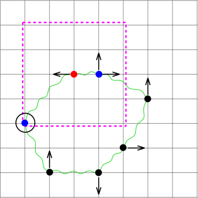
Figure 1: An example of a configuration that satisfies the initial conditions discussed in the text to have a single closed polymer. This is illustrated explicitly for the particle in red: the box of size $2r$ ($r=2$) is indicated by the dashed purple square, and the two other particles inside the box are colored in blue. The same condition holds for all the particles in the system. All the (nearest-neighbor) particle moves allowed by the kinetic constraint are shown for each particle with arrows along the corresponding lattice edge. One particle in this configuration is temporarily frozen (circled blue particle), and its move is subordinated to the move of one of the two particles in its box of size $2r$. Notice that the initial sequence of particles, represented by the wiggly green line, is clearly preserved by the allowed moves.

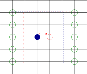
Figure 2: For a model with an $r=2$ box, a monomer can hop in a given direction if the destination site, as well as the ten sites which the old and new box differ by, are empty.

We choose the smallest value of $r$ for which the model behaves like a polymer while allowing for shorter simulation times. The $r=1$ case is too restrictive to model different modes of motion. For example a polymer lying along a straight line is forbidden in the $r=1$ model to undergo one-dimensional translation. We choose $r=2$ as it is found to adequately describe the free polymer dynamics, as shown by our numerical simulations.

Monte Carlo (MC) simulations are used to study the model. A particularly time-efficient algorithm is achieved by storing two representations of the system at each MC step. One consists of the position vector of all the monomers, and the other is the configuration matrix of the lattice, with unoccupied sites having value zero and occupied sites value one. This allows us to chose a monomer at random from the position vector (rather than a site at random from the whole lattice) and quickly determine if the monomer is allowed to move in a randomly chosen direction by checking the values of at most eleven elements (the nearest neighbor site plus the sites by which the old and new box differ) in the configuration matrix. Note that it is possible to define an alternative model by using a circle of radius $r=2$ instead of a square box of side $2r=4$, which would require the same amount of computational effort because the same number of sites, namely ten sites, would enter or leave the circle drawn around the moving monomer.

The $r=2$ model with a square box proved to give consistent results with the ones available in the literature. Namely, the time-averaged radius of gyration squared of the polymer computed for our model in an infinite box scales as $R^{2}\propto N^{1.451\pm 0.084}$, which is consistent with Flory’s theoretical result of $R^{2}\propto N^{\frac{3}{2}}$ Flory:49 . The dynamics of the polymer in unconfined environments is also compatible with the Rouse model to a good approximation. As shown in Fig. 3, the mean square displacement of the center of mass is diffusive with a diffusion constant that scales as $N^{-0.96}$ compared to the $N^{-1}$ theoretical value. Throughout the paper, time and length are measured in units of Monte-Carlo steps and lattice spacings respectively. Only four values of $N=128,256,512,1024$ were used for these consistency checks but the fits were very close to the theoretical predictions. The individual monomer mean square displacement is diffusive at very short times followed by an intermediate-time subdiffusive behavior and a cross-over to a final diffusive behavior at long times as each monomer begins to move with the center of mass. The subdiffusive MSD can be fit with an exponent of $0.5968\pm 0.0008$ over the two-decade interval of $10^{1}<t<10^{3}$ which is consistent with the theoretical value of $\frac{3}{5}$ and the bond fluctuation results Kremer:88 . Because of the cross-over to diffusive behavior at long times the curve fits well to a higher exponent of $0.6516\pm 0.0008$ over the longer interval of $10^{1}<t<10^{6}$.

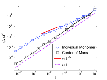
Figure 3: Center of mass and individual monomer mean square displacement of a free polymer. The results are shown for $N=256$.

In the present paper we focus on open and closed polymers without any branching. The close-packing density of such polymers clearly has an upper limit. For a single open chain for example, each monomer except for the two end-points has exactly two box-neighbors. The maximally packed configuration is achieved once the distance along the chain between the consecutive monomers alternates between one and two lattice spacings, and the distance between parallel segments of the folded polymer equals $3$ lattice spacings, as depicted in Fig. 4. If we have $N$ monomers on an $L\times L$ lattice with $(L+1)^{2}$ sites, the fully-packed configuration attains a thermodynamic-limit density $\rho=\frac{N}{(L+1)^{2}}\to\frac{2}{9}$ ($\frac{2}{3^{d}}$ in $d$ dimensions). Note that except for fluctuations at the U-turns, the polymer is completely frozen at close-packing.

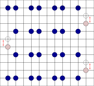
Figure 4: A fully packed configuration of the model described in the text. Notice that only the shaded monomers are allowed to move at any given time.

III Mean square monomer displacement

The question of whether or not placing a self-avoiding polymer in a highly confining environment can freeze its motion can be addressed by measuring the statistical average of the mean square displacement as a function of time

$$c(t)=\langle\frac{1}{N}\sum_{i=1}^{i=N}\left[\vphantom{\sum}\vec{x_{i}}(t+t_{w})-\vec{x_{i}}(t)\right]^{2}\rangle,$$ (2)

where $\vec{x_{i}}$ is the position of the $i$-th monomer and $t_{w}$ is the waiting time between the preparation of the sample and the measurement. Throughout the paper, we denote the ensemble average by $\langle\ldots\rangle$. We prepare random samples with different densities by placing the polymer in a large box and gradually reducing the size of the box. This is achieved by forbidding the monomers to move to the edges of the box, which corresponds to an infinite repulsive potential at the boundary, and removing one vertical and one horizontal edge line once they have become completely empty. After each shrinking process, the system is confined to a smaller square box. Shrinking and measurements are done in series. Specifically, we start from a very low density of $\rho=0.00010$ and after each shrinking step we let the system run for $1000$ Monte-Carlo steps before trying to shrink further. For measurements involving a long waiting time ($t_{w}=10^{7}$ steps), i.e., for densities $\rho\simeq 0.0010,0.050,0.10,0.15$ and $\rho>0.195$, subsequent shrinking steps are preformed starting from the post-measurement configurations. With this method we are able to reach densities of approximately $\rho=0.21$, compared to the limiting theoretical value of $\rho=2/9\simeq 0.222$. At high densities, as shown in Fig. 5, the overall geometry of the polymer resembles that of a compact polymer described by a Hamiltonian path, i.e., a path which visits all sites exactly once, exploring a lattice with lattice spacing three times larger than in the original one. At these high densities our model resembles a semi-flexible polymer because the chain is able to attain a higher packing density in the direction parallel to the backbone (average monomer spacing equal to $\frac{3}{2}$ lattice spacings) than in the direction perpendicular to the backbone (average monomer spacing equal to $3$ lattice spacings) (see Fig. 4).

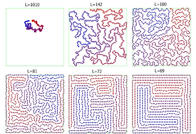
Figure 5: Snapshots of a polymer with $N=1024$ monomers. As the box shrinks, the polymer gets more and more confined. At densities close to full-packing, a geometry resembling that of a compact (Hamiltonian walk) polymer is formed.

Measurements are done with two values of waiting time, $t_{w}=10^{7}$ and $t_{w}=1.1\times 10^{8}$ Monte-Carlo steps over a period of $t=10^{8}$ steps. (For the highest density we used $t=2\times 10^{8}$ instead.) The mean square displacement shows time translation invariance up to the highest densities achieved. We study the behavior of $c(t)$ for $N=128,256,512,1024$ at the densities listed above. The root mean square displacement $\sqrt{c(t)}$ is a measure of how much the monomers have moved. As shown in Fig. 6, $c(t)$ increases with power law behavior and finally saturates with a limiting root mean square displacement of the order of the box size. For very large box sizes (lowest density) as well as very small box sizes (very high densities), the saturation plateau is not always reached within the measurement time. However, the maximum value of $\sqrt{c(t)}$ is still of the same order of the box dimensions. Although the dynamics slows down at high confinement, each monomer manages to move an average distance comparable to the box size over our measurement time $t$. Visually observing the polymer motion, however, clearly shows a more complex scenario where at high densities the overall geometry of the polymer is largely preserved (see Fig. 5). Indeed, we will see that the tangent-tangent correlation function, although time-translation invariant at low and intermediate densities, exhibits signs of aging at higher densities. In the following sections we discuss in detail the shape persistence as well as the mechanisms by which the polymer shape changes as the box size is reduced.

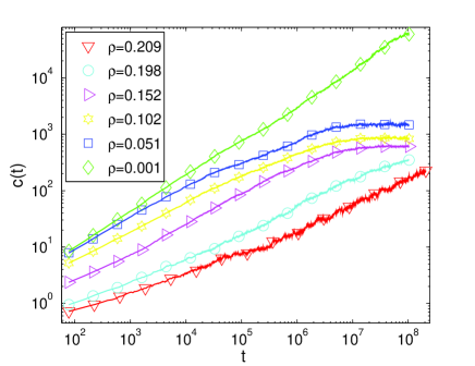
Figure 6: Mean square displacement for $N=256$ and different box sizes (i.e., different densities) as a function of time. The $\rho=0.001$ curve can be fit with a $0.63$ exponent which is close to the intermediate-time regime of the Rouse model. The results for other values of N are qualitatively very similar.

IV Tangent field Correlation

The large values reached by $\sqrt{c(t)}$ within our simulation times even for very high densities indicate that confinement does not freeze the motion of the monomers. The overall shape or geometry of the polymer, however, exhibits global persistence at high densities as observed via direct visualization of the dynamics. In order to systematically study shape persistence and reshaping, we introduce the concept of a tangent field, a vector field defined on the entire lattice which captures the overall shape of the polymer. We define the instantaneous tangent field as

$$\vec{s}_{\textrm{inst}}(\vec{x},t)=\left\{\begin{array}[]{ll}\vec{x}_{i+1}(t)-\vec{x}_{i-1}(t)&\textrm{if $\vec{x}=\vec{x}_{i}(t)$}\\ \vec{0}&\textrm{otherwise},\end{array}\right.$$ (3)

$\vec{x}_{i}(t)$ being the position of monomer $i$ at time $t$. The tangent field is defined in a symmetric way so that labeling the monomers in reverse order only changes the direction of the field. In an open chain, the definition needs to be modified at the end points. Note that the tangent field is indexed by a position in space and not by a monomer number; this allows us to compare the shapes at different times, independently of the monomer motion. Since local vibrations of the polymer do not change the overall geometry, we seek a quantity that is insensitive to these vibrations. Coarse-graining the field by time averaging over a carefully chosen interval removes the local vibrations and results in a smeared field $\vec{s}_{\vec{x}}(t)$ which captures the overall geometry, as shown in Fig. 7. We have chosen the time interval to be $75$ Monte Carlo steps (or $75\times N$ single monomer attempts) which is sufficient to allow for several vibrations. Since the success rate of the Monte Carlo attempts at high density is found to be around $1/10$, this interval corresponds to roughly $7$ moves per monomer.

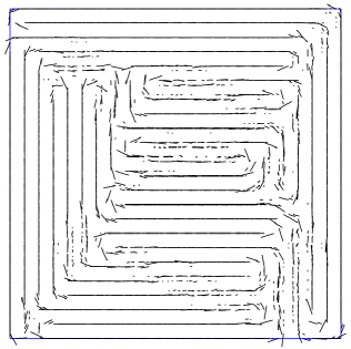
Figure 7: An example of the coarse-grained tangent field $\vec{s}_{\vec{x}}(t)$

In terms of the coarse-grained tangent field defined above, we define the tangent-tangent correlation function

$$c_{s}(t,t_{w})=\langle\frac{1}{N}\sum_{\textrm{all}\,\vec{x}}\left[\vphantom{\sum}\vec{s}_{\vec{x}}(t+t_{w})\cdot\vec{s}_{\vec{x}}(t_{w})\right]\rangle$$ (4)

as a measure of the overlap of the tangent field at times $t+t_{w}$ and $t_{w}$.

As shown in Fig. 8, $c_{s}(t,t_{w})$ decays as a power low in $t$ for very low densities. As the density increases, a second time scale emerges and at the highest densities we clearly see an initial decay followed by a broad plateau and a secondary decay. (Notice the use of a logarithmic scale on both axes.) The time-averaging of the tangent field hides the fast mode responsible for the initial decay and causes the correlation to have a smaller initial value at lower densities. The correlation function (4) does not depend on the value of $N$ at low densities, as seen in Fig. 9, while at higher densities we observe broader plateaux and longer decorrelation times as the number of monomers $N$ is increased.

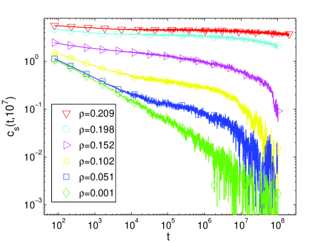
Figure 8: Tangent-tangent correlation function for $256$ monomers and different box sizes. The $\rho=0.001$ curve fits well to a power law of exponent $0.42$. Note that the correlation functions are not normalized.

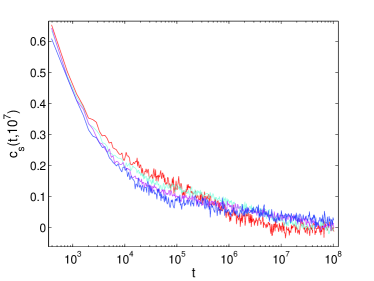
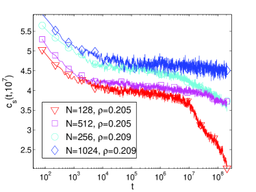
Figure 9: The tangent-tangent correlation function for four different polymer sizes. Top: At low density $\rho=0.05$, the curves are independent of $N$. Bottom: At the highest achieved density $\rho\simeq 0.20-0.21$, the width of the emergent plateau increases with $N$

To check for time-translation invariance, we ran the simulations two more times after increasing the waiting time $t_{w}$ by an order of magnitude each time. The mean square displacement exhibits time-translation invariance at all densities. For the tangent-tangent correlation function, however, time-translation invariance is respected at low densities but violated at the highest densities where a broad plateau emerges. It appears that at high densities the average distance between monomers slowly evolves with time, so that the initial value of the tangent-tangent correlation function $c_{s}(0,t_{w})$ depends on $t_{w}$. If we normalize the correlation function using its value at the beginning of the measurement and plot $c_{s}(t,t_{w})/c_{s}(0,t_{w})$ as a function of time, the violation of time-translation invariance suggests the existence of aging effects, a comprehensive study of which is beyond the scope of the present paper. For $t_{w}=1.01\times 10^{9}$, the system has almost equilibrated but there is still a systematic shift toward longer times compared with the $t_{w}=1.1\times 10^{8}$ correlation function. Fig. 10 summarizes the above observations. Moreover, Fig. 9 suggests longer equilibration times for larger systems and in the thermodynamic limit ($N\rightarrow\infty$) the aging effects are expected to survive for arbitrarily large $t_{w}$.

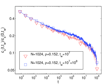
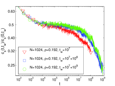
Figure 10: The normalized tangent-tangent correlation function $c_{s}(t,t_{w})/c_{s}(0,t_{w})$ vs. time for different waiting times shown in log-log plots. Top: Up to intermediate densities, before the appearance of a clear plateau, time translation invariance is not broken. Bottom: At higher densities, where a broad plateau has emerged, we observe that the second decay occurs at a longer time scale. With increasing the waiting times the correlation function approaches equilibrium but there is still a systematic shift between $t_{w}\approx 10^{9}$ and $t_{w}\approx 10^{8}$ curves indicating slower decay for the older system.

V Tangent-Displacement correlation

As seen in the previous sections, confinement slows down the motion of individual monomers in a polymer chain, but it does not fundamentally change the characteristics of their mean square displacement. It does, however, have a profound effect on reshaping. Without any reshaping, the only possible motion can happen via reptation, i.e., when the monomers move back and forth along a fixed path. With the exception of the unlikely event of the two end-points finding each other, reptation without reshaping is not possible in open chains. Indeed, by studying closed loops in detail we do find that longitudinal diffusion is the main mechanism for motion at high densities. The existence of large root mean square displacements in strongly confined open chains and in the absence of major reshaping can be explained by noting that local reshaping events with only a minor contribution to the tangent-tangent decorrelation allow for global monomer motion through a reptation-like process. Fig. 11 shows one instance of such behavior in a particularly mobile realization. The mechanisms shown in Fig. 11, namely end-point initiated reptation and ”fingering” events, are observed in other realizations as well. A finger is formed when the chain makes a 180-degree bend resulting in two adjacent segments of the polymer running antiparallel to each other. A fingering event occurs when a finger retracts making room for the extension of another finger. Even in the case of closed loops where pure reptation is possible, reptation is usually accompanied by local fingering events as shown in Fig. 12. To explicitly quantify the contribution of reptation to highly confined motion, we define tangent-displacement and normal-displacement correlation functions as follows:

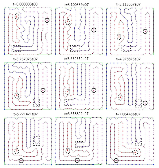
Figure 11: Snapshots of a particularly mobile realization of a $256$-monomer chain at density $\rho=0.209$. Fingering events are observed as well of end-point reptation accompanied by local rearrangements. An end-point initiated reptation is highlighted with a dashed ellipse at the moving end-point. The dashed rectangle shows the tip of a finger which participates in a fingering event during which the tagged monomer shown with a solid circle, for example, moves through reptation.

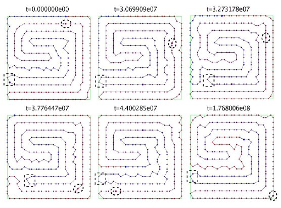
Figure 12: Snapshots of a realization with $256$ monomers arranged in a single closed polymer chain, at density $\rho=0.209$. Pure reptation and fingering events are visibly responsible for monomer motion. The dashed rectangle highlights the tip of a finger taking part in a fingering event. The dashed ellipse shows the reptational motion of a tagged monomer.

$$c_{t}(t) = \langle\frac{1}{N}\sum_{i=1}^{N}\left\{\vphantom{\sum}\frac{\vec{s}_{\vec{x}_{i}}(t_{w})}{|\vec{s}_{\vec{x}_{i}}(t_{w})|}\cdot\left[\vphantom{\sum}\vec{x}_{i}(t_{w}+t)-\vec{x}_{i}(t_{w})\right]\right\}^{2}\rangle$$ (5)

$$c_{n}(t) = \langle\frac{1}{N}\sum_{i=1}^{N}\left\{\vphantom{\sum}\frac{\vec{n}_{\vec{x}_{i}}(t_{w})}{|\vec{n}_{\vec{x}_{i}}(t_{w})|}\cdot\left[\vphantom{\sum}\vec{x}_{i}(t_{w}+t)-\vec{x}_{i}(t_{w})\right]\right\}^{2}\rangle,$$ (6)

where $\vec{n}$ is the normal field defined as $\vec{n}_{\vec{x}}(t)=\hat{z}\times\vec{s}_{\vec{x}}(t)$ and the polymer – and therefore $\vec{s}_{\vec{x}}(t)$ – belongs to the $xy$ plane. By comparison with Eq. (2), one can show that

$$c(t)=c_{t}(t)+c_{n}(t).$$ (7)

Therefore, the correlation functions (6) and (5) are the contributions to the mean square displacement due to the transverse and longitudinal motion relative to the initial polymer orientation. At very high densities and up to time scales smaller than the beginning of the secondary decay in the tangent-tangent correlation function Eq. (4), $c_{t}$ is a good measure of the reptational contribution to the confined motion. This is due to the fact that over such time scales the polymer shape is largely preserved. Additionally, over the same time scales the mean square displacement is smaller than the average chain length between major bends, which as seen in Fig. 11 is a large fraction of the box size. If the polymer undergoes major reshaping or the monomers move through the bends of the folded polymer, reptation would no longer be equivalent to the motion along the original orientation.

Let us define $f$ as a measure of the anisotropy of the motion with respect to the longitudinal and transverse directions,

$$f(t)=\frac{c_{t}(t)-c_{n}(t)}{c(t)}.$$ (8)

We have $c_{t}(t)/c(t)=(1+f(t))/2$ and $c_{n}(t)/c(t)=(1-f(t))/2$, where $f$ ranges from $-1$ to $+1$. A large value of $f$ clearly indicates a motion primarily due to reptation. As shown in semi-logarithmic scale in Fig. 13, $f$ reaches a maximum value of $0.8$ at short time scales, demonstrating that reptation-like motion is the primary contributor to monomer displacement. We also observe that the maximum of $f$ increases as the number of monomers $N$ is increased, consistent with the fact that the width of the plateau becomes monotonically larger and larger with $N$.

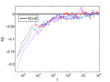
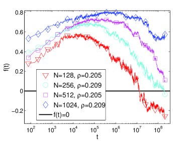
Figure 13: Top: At the lowest density studied $\rho\simeq 0.001$, the function $f$ is independent of the number of monomers and approaches zero monotonically (i.e., the motion is isotropic at intermediate and large time scales). Bottom: At the highest densities achieved $\rho\simeq 0.20-0.21$, the function $f$ reaches very large positive values before decreasing again towards zero. For short polymers $f(t)$ goes down to negative values at large times. Here we ignore the causes of this observation because as explained in the text, $f(t)$ is a good measure of the anisotropy of the motion only up to certain time scales.

VI Conclusions

As the size of the confining box around a polymer is reduced, the monomer density makes it increasingly difficult for the polymer to move. However, the effect on the polymer movement is not isotropic. The transverse fluctuations are strongly suppressed due to the proximity of monomers that may be greatly separated along the chain backbone. This is in contrast to motion parallel to the chain backbone where, due to the connectivity constraint, the monomer density is very similar for the confined and unconfined chains. While longitudinal motion is sub-dominant in the free chain, it is the primary mode of monomer diffusion when the density becomes high enough to suppress the transverse fluctuations.

The emergence of motion parallel to the chain backbone as the dominant mode of diffusion is similar to what occurs in a polymer solution when the density is increased to form a melt. However, the longitudinal diffusion observed here differs from the classic reptation picture in that the motion is not necessarily initiated at the chain ends but it can also be triggered by fingering events. The prevalence of fingering reptation over end-initiated reptation is due to three factors. First, the two-dimensional nature of our system imposes topological constraints that severely limit the mobility of the chain ends. Second, a single confined chain has only two end-points, while the number of fingers it can have grows with the system size. Third, the compact configuration due to the confinement forces the creation of more fingering structures relative to the extended polymer structures found in melts.

The peculiarities of the dynamics of a single chain in extreme confinement (high density limit) leads to an interesting effect: monomers can diffuse through large distances comparable to the box size within time scales for which the overall shape of the polymer is, nevertheless, largely preserved. While monomer displacement exhibits a smooth power law behavior in time at all densities, the tangent-tangent correlation function develops a secondary decay at high densities. This decay takes place at longer time scales for older systems, suggestive of aging phenomena. We thus find glass-like behavior in the overall geometry concurrently with non-glassy monomer motion. Despite significant persistence of geometry, monomer displacement can reach large values relative to its saturation value over the same time scales because local rearrangements cause monomers to flow even in parts of the system where no reshaping is taking place.

The two dimensional lattice model presented here is a largely simplified one. However, we believe that this model yields considerable insight into the generic properties of confined polymers. Namely, reptational or longitudinal motion is identified as the primary mechanism for motion at high densities and extreme confinement is found to primarily suppress changes in the overall geometry of the polymer rather than the monomer motion.

Appendix: Closed chains

Closed chains can be studied using the same correlation functions. The only subtlety with closed chains is the existence of a non-trivial background in finite systems. The background has to do with the topology of closed loops and must be subtracted from the tangent-tangent correlation function. Suppose that the monomers in the chain are initially indexed clockwise or anti-clockwise. The dynamics cannot change the chirality of the loop in two dimensions. Therefore, all the outer segments of the polymer running parallel to the walls of the box have correlated tangent fields. Using an ensemble with random chirality does not remove the problem because each realization, whether clockwise or anti-clockwise, would contribute a positive value to the correlation function.

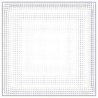
Figure 14: The background tangent field for $N=256$ monomers in a box of size $L=49$. The relative scale between the field vectors reflects the actual values of the tangent-tangent field (an overall scale factor has been introduced to enhance visibility). Notice that the average field at the boundary does not vanish.

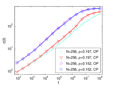
Figure 15: The mean square displacements of closed polymers (CP) and open polymers (OP) are identical at low and intermediate densities. At high densities closed polymers seem to reach the saturation value faster.

One can correct for this effect as follows. For an ensemble with a given chirality, let us call the equilibrium tangent-field background $\vec{s}_{\textrm{ave}}(\vec{x})$. We can then modify the tangent-tangent correlation function by subtracting this background field.

$$c_{s,\textrm{loop}}(t,t_{w})=\langle\frac{1}{N}\sum_{\textrm{all}\,\vec{x}}\left[\vphantom{\sum}\vec{s}_{\vec{x}}(t+t_{w})-\vec{s}_{\textrm{ave}}(\vec{x})\right]\cdot\left[\vphantom{\sum}\vec{s}_{\vec{x}}(t_{w})-\vec{s}_{\textrm{ave}}(\vec{x})\right]\rangle.$$ (9)

The equilibrium background can be obtained at low densities via Monte Carlo simulations, using realizations with the same chirality and averaging over time and ensemble. This approach becomes less and less reliable as the density increases and glassy behavior arises, because each realization is essentially stuck in a small region of configuration space over the measurement time scales. Fig. 14 shows the background tangent field at an intermediate density $\rho=0.1$. The modified tangent-tangent correlation function (9) and the mean square displacement were measured for a closed loop of $N=256$ monomers and no qualitative difference was observed in comparison to open chains. Also $f(t)$ behaves similarly in the two cases, reaching high values at high densities for closed chains as well as open chains. As shown in Fig. 15, the mean square displacement for closed chains at high densities reaches its saturation value faster than for open chains, whereas at low and intermediate densities they are identical.

References

- (1) T. Cremer and C. Cremer, Nature Rev. Gen. 2, 292-301 (2001).
- (2) G.M. Whitesides, Nature 442, 368-373 (2006).
- (3) P.G. de Gennes, Scaling concepts in polymer physics, Cornell University Press (1979).
- (4) M. Muthukumar, Phys. Rev. Lett. 86, 3188 - 3191 (2001).
- (5) S.M. Bezrukov, I. Vodyanoy, R.A. Brutan, and J.J. Kasianowicz, Macromolecules 29, 8517 (1996).
- (6) D. Nykypanchuk, H.H. Strey, D.A. Hoagland, Science 297, 987 - 990 (2002).
- (7) J. Kalb, B. Chakraborty, cond-mat/0702152.
- (8) A. J. Spakowitz and Z.-G. Wang, Biophys. J., 88, 3912 (2005).
- (9) J.A. Forrest and K. Dalnoki-Veress, Adv. Colloid and Interface Sci. 94, 167 (2001).
- (10) J.L. Keddie, R.A.L. Jones, and R.A. Cory, Europhys. Lett. 27, 59 (1994).
- (11) P.G. de Gennes, Eur. Phys. J. E 2, 201 (2000).
- (12) K.L. Ngai, A.K. Rizos, and D.J. Plazek, J. Non-cryst. Sol. 235, 435 (1998).
- (13) Q. Jiang, H.X. Shi, and J.C. Li, Thin Solid Films 354, 283 (1999).
- (14) K. Kremer and I. Carmesin, Macromolecules 21, 2819 (1988).
- (15) F. Ritort and P. Sollich, Advances in Physics 52, 219 (2003).
- (16) W. Kob and H.C. Andersen, Phys. Rev. E 48, 4364 (1993).
- (17) C. Toninelli, G. Biroli and D. Fisher, Phys. Rev. Lett. 92, 185504 (2004).
- (18) P.J. Flory, J. Chem. Phys. 17, 303 (1949).
- (19) T. Odijk Macromolecules 16, 1340-1344 (1983)