A Renormalization group approach for highly anisotropic 2D Fermion systems: application to coupled Hubbard chains

Abstract

I apply a two-step density-matrix renormalization group method to the anisotropic two-dimensional Hubbard model. As a prelude to this study, I compare the numerical results to the exact one for the tight-binding model. I find a ground-state energy which agrees with the exact value up to four digits for systems as large as $24\times 25$. I then apply the method to the interacting case. I find that for strong Hubbard interaction, the ground-state is dominated by magnetic correlations. These correlations are robust even in the presence of strong frustration. Interchain pair tunneling is negligible in the singlet and triplet channels and it is not enhanced by frustration. For weak Hubbard couplings, interchain non-local singlet pair tunneling is enhanced and magnetic correlations are strongly reduced. This suggests a possible superconductive ground state.

I Introduction

Quasi-one dimensional organic reviewOC and inorganic reviewIOC materials have been the object of an important theoretical interest for the last three decades. The essential features of their phase diagram may be captured by the anisotropic Hubbard model (AHM),

$$H=-t_{\parallel}\sum_{i,l,\sigma}(c_{i,l,\sigma}^{\dagger}c_{i+1,l,\sigma}+h.c.)+U\sum_{i,l}n_{i,l,\uparrow}n_{i,l,\downarrow}$$

$$+V\sum_{i,l,\sigma}n_{i,l,\sigma}n_{i+1,l,\sigma}-\mu\sum_{i,l,\sigma}n_{i,l,\sigma}$$

$$-t_{\perp}\sum_{i,l,\sigma}(c_{i,l,\sigma}^{\dagger}c_{i,l+1,\sigma}+h.c.).$$ (1)

or a more general Hubbard-like model including longer range Coulomb interactions. The indices $i$ and $l$ label the sites and the chains respectively. For these highly anisotropic materials, $t_{\perp}\ll t_{\parallel}$. Over the years, the AHM has remained a formidable challenge to condensed-matter theorists. Some important insights on this model or its low energy version, the g-ology model, have been obtained through the work of Bourbonnais and Caron bourbonnais ; giamarchi and others. They used a perturbative renormalization group approach to analyze the crossover from 1D to 2D at low temperatures. More recently, Biermann et al. bierman applied the chain dynamical mean-field approach to study the crossover from Luttinger liquid to Fermi liquid in this model. Despite this important progress, crucial information such as the ground-state phase diagram, or most notably, whether the AHM displays superconductivity, are still unknown. So far it has remained beyond the reach of numerical methods such as the exact diagonalization (ED) or the quantum Monte Carlo (QMC) methods. ED cannot exceed lattices of about $4\times 5$. It is likely to remain so for many years unless there is a breakthrough in quantum computations. The QMC method is plagued by the minus sign problem and will not be helpful at low temperatures. The small value of $t_{\perp}$ implies that, in order to see the 2D behavior, it will be necessary to reach lower temperatures than those usually studied for the isotropic 2D Hubbard model. Hence, even in the absence of the minus sign problem, in order to work in this low temperature regime, the QMC algorithm requires special stabilization schemes which lead to prohibitive cpu time. white-qmc

II Two-step DMRG

I have shown in Ref. moukouri-TSDMRG, that this class of anisotropic models may be studied using a two-step density-matrix renormalization group (TSDMRG) method. The TSDMRG method is a perturbative approach in which the standard 1D DMRG is applied twice. In the first step, the usual 1D DMRG method white is applied to find a set of low lying eigenvalues $\epsilon_{n}$ and eigenfunctions $|\phi_{n}\rangle$ of a single chain. In the second step, the 2D Hamiltonian is then projected onto the basis constructed from the tensor product of the $|\phi_{n}\rangle$’s. This projection yields an effective one-dimensional Hamiltonian for the 2D lattice,

$$\tilde{H}\approx\sum_{[n]}E_{\parallel[n]}|\Phi_{\parallel[n]}\rangle\langle\Phi_{\parallel[n]}|-t_{\perp}\sum_{i,l,\sigma}(\tilde{c}_{i,l,\sigma}^{\dagger}\tilde{c}_{i,l+1,\sigma}+h.c.)$$ (2)

where $E_{\parallel[n]}$ is the sum of eigenvalues of the different chains, $E_{\parallel[n]}=\sum_{l}{\epsilon_{n_{l}}}$; $|\Phi_{\parallel[n]}\rangle$ are the corresponding eigenstates, $|\Phi_{\parallel[n]}\rangle=|\phi_{n_{1}}\rangle|\phi_{n_{2}}\rangle...|\phi_{n_{L}}\rangle$; $\tilde{c}_{i,l,\sigma}^{\dagger}$, $\tilde{c}_{i,l,\sigma}$, and $\tilde{n}_{i,l,\sigma}$ are the renormalized matrix elements in the single chain basis. They are given by

$$(\tilde{c}_{i,l,\sigma}^{\dagger})^{n_{l},m_{l}}=(-1)^{n_{i}}\langle\phi_{n_{l}}|{c}_{i,l,\sigma}^{\dagger}|\phi_{m_{l}}\rangle,$$ (3)

$$(\tilde{c}_{i,l,\sigma})^{n_{l},m_{l}}=(-1)^{n_{i}}\langle\phi_{n_{l}}|{c}_{i,l,\sigma}|\phi_{m_{l}}\rangle,$$ (4)

$$(\tilde{n}_{i,l,\sigma})^{n_{l},m_{l}}=\langle\phi_{n_{l}}|{n}_{i,l,\sigma}|\phi_{m_{l}}\rangle,$$ (5)

where $n_{i}$ represents the total number of fermions from sites $1$ to $i-1$. For each chain, operators for all the sites are stored in a single matrix

$$\tilde{c}_{l,\sigma}^{\dagger}=(\tilde{c}_{1,l,\sigma}^{\dagger},...,\tilde{c}_{L,l,\sigma}^{\dagger}),$$ (6)

$$\tilde{c}_{l,\sigma}=(\tilde{c}_{1,l,\sigma},...,\tilde{c}_{L,l,\sigma}),$$ (7)

$$\tilde{n}_{l,\sigma}=(\tilde{n}_{1,l,\sigma},...,\tilde{n}_{L,l,\sigma}).$$ (8)

Since the in-chain degrees of freedom have been integrated out, the interchain couplings are between the block matrix operators in Eq.( 6, 7) which depend only on the chain index $l$. In this matrix notation, the effective Hamiltonian is one-dimensional and it is also studied by the DMRG method. The only difference compared to a normal 1D situation is that the local operators are now $ms_{2}\times ms_{2}$ matrices, where $ms_{2}$ is the number of states kept during the second step.

The two-step method has previously been applied to anisotropic two-dimensional Heisenberg models.moukouri-TSDMRG In Ref. moukouri-TSDMRG2, , it was applied to the $t-J$ model but due to the absence of an exact result in certain limits, it was tested against ED results on small ladders only. A systematic analysis of its performance on a fermionic model on 2D lattices of various size has not been done. In this paper, as a prelude to the study of the AHM, I will apply the TSDMRG to the anisotropic tight-binding model on a 2D lattice, i.e., model (1) with $U=V=0$. I perform a comparison with the exact result of the tight-binding model. I was able to obtain agreement for the ground-state energies on the order of $10^{-4}$ for lattices of up to $24\times 25$. I then discuss how these calculations may be extended to the interacting case, before presenting the $U\neq 0$ results.

III Warm up: the tight-binding model

The tight-binding Hamiltonian is diagonal in the momentum space, the single particle energies are,

$$\epsilon_{k}=-2t_{\parallel}cosk_{x}-2t_{\perp}cosk_{y}-\mu,$$ (9)

with $k=(k_{x},k_{y})$, $k_{x}=n_{x}\pi/(L_{x}+1)$ and $k_{y}=n_{y}\pi/(L_{y}+1)$ for open boundary conditions (OBC); $L_{x}$, $L_{y}$ are respectively the linear dimensions of the lattice in the parallel and transverse directions. The ground-state energy of an $N$ electron system is obtained by filling the lowest states up to the Fermi level, $E_{[0]}(N)=\sum_{k<k_{F}}\epsilon_{k}$. However in real space, this problem is not trivial and it constitutes, for any real space method such as the TSDMRG, a test having the same level of difficulty as the case with $U\neq 0$. This is because the term involving $U$ is diagonal in real space and the challenge of diagonalizing the AHM arises from the hopping term.

I will study the tight-binding model at quarter filling, $N/L_{x}L_{y}=1/2$, the nominal density of the organic conductors known as the Bechgaard salts. Systems of up to $L_{x}\times L_{y}=L\times(L+1)=24\times 25$ will be studied. During the first step, I keep enough states ($ms_{1}$ is a few hundred) so that the truncation error $\rho_{1}$ is less than $10^{-6}$. I target the lowest state in each charge-spin sectors $N_{x}\pm 2,~{}N_{x}\pm 1,~{}N_{x}$ and $S_{z}\pm 1,~{}S_{z}\pm 2$, $N_{x}$ is the number of electrons within the chain. It is fixed such that $N_{x}/L_{x}=1/2$. There is a total of $22$ charge-spin states targeted at each iteration.

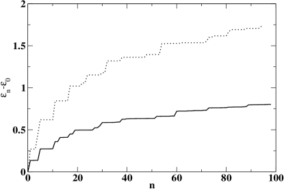
Figure 1: Low-lying states of the 1D tight-binding model (full line) and of the 1D Heisenberg spin chain (dotted line) for $L=16$ and $ms_{2}=96$.

For the tight-binding model, the chains remain disconnected if $t_{\perp}<\epsilon_{0}(N_{x}+1)-\epsilon_{0}(N_{x})$ or $t_{\perp}<\epsilon_{0}(N_{x})-\epsilon_{0}(N_{x}-1)$, where $N_{x}$ is the number of electons on single chain. In order to observe transverse motion, it is necessary that at least $t_{\perp}\gtrsim\epsilon_{0}(N_{x}+1)-\epsilon_{0}(N_{x})$ and $t_{\perp}\gtrsim\epsilon_{0}(N_{x})-\epsilon_{0}(N_{x}-1)$. These two conditions are satisfied only if $\mu$ is appropietly chosen. The values listed in Table (1) corresponds to $\mu=(\epsilon_{0}(N_{x}+1)-\epsilon_{0}(N_{x}-1))/2$. This treshold varies with $L$. I give in Table (1) the values of $t_{\perp}$ chosen for different lattice sizes. In principle, for the TSDMRG to be accurate, it is necessary that $\Delta\epsilon=\epsilon_{n_{c}}-\epsilon_{0}$, where $\epsilon_{n_{c}}$ is the cut-off, be such that $\Delta\epsilon/t_{\perp}\gg 1$. But in practice, I find that I can achieve accuracy up to the fourth digit even if $\Delta\epsilon/t_{\perp}\approx 5$ using the finite system method. Five sweeps were necessary to reach convergence. Note that this conclusion is somewhat different from my earlier estimate of $\Delta\epsilon/t_{\perp}\approx 10$ for spin systems. moukouri-TSDMRG2 This is because in Ref. moukouri-TSDMRG2, , I used the infinite system method during the second step.

The ultimate success of the TSDMRG depends on the density of the low-lying states in the 1D model. For fixed $ms_{2}$ and $L$, it is, for instance, easier to reach larger $\Delta\epsilon/J_{\perp}$ in the anisotropic spin one-half Heisenberg model, studied in Ref. moukouri-TSDMRG, , than $\Delta\epsilon/t_{\perp}$ for the tight-binding model as shown in Fig.1. For $L=16$, $ms_{2}=96$, and $J_{\perp}=t_{\perp}=0.15$, I find that $\Delta\epsilon/J_{\perp}\approx 10$, while $\Delta\epsilon/t_{\perp}\approx 5$. Hence, the TSDMRG method will be more accurate for a spin model than for the tight-binding model. Using the infinite system method during the second step on the anisotropic Heisenberg model with $J_{\perp}=0.1$, I can now reach an agreement of about $10^{-6}$ with the stochastic QMC method.

	$8\times 9$	$16\times 17$	$24\times 25$
$t_{\perp}$	0.28	0.15	0.1
$\mu$	-1.2660	-1.3411	-1.3657
$\Delta\epsilon/t_{\perp}$	6.42	5.40	5.78

Table 1: Transverse hopping and chemical potential used in the simulations for different lattice sizes

Two possible sources of error can contribute to reduce the accuracy in the TSDMRG with respect to the conventional DMRG. They are the truncation of the superblock from $4\times ms_{1}$ states to only $ms_{2}$ states and the use of three blocks instead of four during the second step. In Table (2) I analyze the impact of the reduction of the number of states to $ms_{2}$ for three-leg ladders. The choice of three-leg ladders is motivated by the fact that at this point, the TSDMRG is equivalent to the exact diagonalization of three reduced superblocks. It can be seen that as far as $t_{\perp}\gtrsim\epsilon_{0}(N_{x}+1)-\epsilon_{0}(N_{x})$ and $t_{\perp}\gtrsim\epsilon_{0}(N_{x})-\epsilon_{0}(N_{x}-1)$, the TSDMRG at this point is as accurate as the 1D DMRG. Note that the accuracy remains nearly the same irrespective of $L$ as far as the ratio $\Delta\epsilon/t_{\perp}$ remains nearly constant. Since $\Delta\epsilon$ decreases when $L$ increases, $t_{\perp}$ must be decreased in order to keep the same level of accuracy for fixed $ms_{2}$. In principle, following this prescription, much larger systems may be studied. $\Delta\epsilon/t_{\perp}$ does not have to be very large, in this case it is about $5$, to obtain very good agreement with the exact result.

$ms_{2}$	$8\times 3$	$16\times 3$	$24\times 3$
$64$	-0.241524	-0.211929	0.204040
Exact	-0.241524	-0.211931	0.204049

Table 2: Ground-state energies of three-leg ladders.

The second source of error is related to the fact that the effective single site during the second step is now a chain having $ms_{2}$ states, I am thus forced to use three blocks instead of four to reduce the computational burden. In Table (3), it can be seen that this results in a reduction in accuracy of about two orders of magnitude with respect to those of three leg-ladders. These results are nevertheless very good given the relatively modest computer power involved. All calculations were done on a workstation.

$ms_{2}$	$8\times 9$	$16\times 17$	$24\times 25$
$64$	-0.24761	-0.21401	0.20504
$100$	-0.24819	-0.21414	0.20509
$120$	-0.24832	-0.21419
Exact	-0.24857	-0.21432	0.20519

Table 3: Ground-state energies for different lattice sizes; a single state was targeted in the second step.

The DMRG is less accurate when three blocks are used instead of four. This can be understood by applying the following view on the formation of the reduced density matrix. The construction of the reduced density matrix may be regarded as a linear mapping $u_{\Psi}:~{}{\bf F^{*}}\rightarrow{\bf E}$, where ${\bf E}$ is the system, ${\bf F}$ is the environment and, ${\bf F^{*}}$ is the dual space of ${\bf F}$. Using the decomposition of the superblock wave function $\Psi_{[0]}=\sum_{i}\phi_{i}^{L}\otimes\phi_{i}^{R}$, with $\phi_{i}^{L}\in{\bf E}$ and $\Phi_{i}^{R}\in{\bf F}$, for any $\phi^{*}\in F^{*}$,

$$u_{\Psi}(\phi^{*})=\sum_{i=1}\langle\phi^{*}|\phi_{i}^{R}\rangle\phi_{i}^{L}.$$ (10)

Let $|k\rangle,~{}k=1,...dim{\bf E}$ and $|l\rangle,~{}l=1,...dim{\bf F}$ be the basis of ${\bf E}$ and ${\bf F}$ respectively. Then, $|l\rangle$ has a dual basis $\langle l^{*}|$ such that $\langle l^{*}|l\rangle=\delta_{l,l^{*}}$. The matrix elements of $u_{\Psi}$ in this basis are just the coordinates of the superblock wave function $\Phi_{[0]_{k,l}}$. The rank $r$ of this mapping, which is also the rank of the reduced density matrix is always smaller or equal to the smallest dimension of ${\bf E}$ or ${\bf F}$, $r<Min(dim{\bf E},dim{\bf F})$. Hence, if $ms_{2}$ states are kept in the two external blocks, the number of non-zero eigenvalues of $\rho$ cannot be larger than $ms_{2}$. Consequently, some states which have non-zero eigenvalues in the normal four block configuration will be missing. A possible cure to this problem is to target additional low-lying states above $\Psi_{[0]}(N)$. The weight of these states in $\rho$ must be small so that their role is simply to add the missing states not to be described accurately themselves. A larger weight on these additional states would lead to the reduction of the accuracy for a fixed $ms_{2}$. In table (4), I show the improved energies when, besides the ground state, I target the lowest states of the spin sectors $S_{z}=-1$ and $S_{z}=+1$ with $N$ electrons. The weights were respectively $0.995$, $0.0025$, and $0.0025$ for the three states. This lowers $E_{[0]}(N)$ in all cases, but the gain does not appear to be spectacular. But I do not know whether this is due to my choice of perturbation of $\rho$ or whether even the algorithm with four blocks would not yield better $E_{[0]}(N)$. If the lowest sectors with $N+1$ and $N-1$ electrons which have $S_{z}=\pm 0.5$ are projected instead, I find that the results are similar to those with $S_{z}=\pm 1$ sectors, there are possibly many ways to add the missing states. A more systematic approach to this problem has recently been suggested. white2 It is based on using a local perturbation to build a correction to the density matrix from the site at the edge of the system. Here, such a perturbation would be $\Delta\rho=\alpha c_{l}^{\dagger}\rho c_{l}$, where $\alpha$ is a constant, $\alpha\approx 10^{-3}-10^{-2}$, and $c_{l}^{\dagger},~{}c_{l}$ are the creation and annihilation operators of the chain at the edge of the system. This type of perturbation resulted in an accuracy gain of more than an order of magnitude in the case of a spin chain. white2 The three block method was found to be on par with the four block method. It will be interesting to see in a future study how this type of local perturbation performs within the TSDMRG.

$ms_{2}$	$8\times 9$	$16\times 17$
$64$	-0.24803	-0.21401
$100$	-0.24828	-0.21417
Exact	-0.24857	-0.21432

Table 4: Ground-state energies for different lattice sizes; three states were targeted in the second step: the ground state itself and the lowest states of $S_{z}=0$ and $S_{z}=1$ sectors.

To conclude this section, as a first step to the investigation of interacting electron models, I have shown that the TSDMRG can successfuly be applied to the tight-binding model. The agreement with the exact result is very good and can be improved since the computational power involved in this study was modest. The extension to the AHM with $U\neq 0$ is straightforward. There is no additional change in the algorithm since the term involving $U$ is local and thus treated during the 1D part of the TSDMRG. The role of $U$ is to reduce $\Delta\epsilon$ as shown in Fig.2. For fixed $L$ and $ms_{2}$, $\Delta\epsilon$ decreases linearly with increasing $U$. For $L=16$ and $ms_{2}=128$, I anticipate that for $U\lesssim 3$ the interacting system results will be on the same level or better than those of the non-interacting case with $ms_{2}=100$ for the same value of $L$.

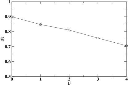
Figure 2: Width $\Delta\epsilon$ for the low-lying states of the 1D Hubbard chain as function of $U$ for $L=16$ and $ms_{2}=128$.

IV Ground-state properties of coupled Hubbard chains

I now proceed to the study of $U\neq 0$. One of the main motivations for such a study is the possibility to gain insight into the mechanism of superconductivity in quasi 1D systems. The mechanism of superconductivity in the quasi 1D organic materials Bechgaard and Fabre salts, is still an open issue. dupuis Since these materials are 1D above a crossover temperature $T_{x}\approx t_{\perp}/\pi$, it is broadly accepted that the starting point for the the understanding of their low $T$ behavior should be pure 1D physics. The occurence of the low $T$ ordered phases is driven by the interchain hopping $t_{\perp}$. Two main hypotheses have been suggested concerning superconductivity. The first hypothesis (see a recent review in Ref. dupuis, ) relies on a more conventional physics: $t_{\perp}$ drives the system to a 2D electron gas which is an anisotropic Fermi liquid which becomes superconductive through a conventional BCS mechanism. However, it has been argued emery that given the smallness of $t_{\perp}$, the resulting electron-phonon coupling would not be enough to account for the observed $T_{c}$. The second hypothesis, which has gained strength over the years given the absence of a clear phonon signature, is that the pairing mechanism originates from an exchange of spin fluctuation. emery

Interest in this issue was recently revived by the NMR Knight shift experimental finding that the symmetry of the Cooper pairs is triplet lee in $(TMTSF)_{2}(PF)_{6}$. No shift was found in the magnetic susceptibility at the transition for measurement made under a magnetic field of about 1.4 Tesla. A triplet pairing scenario was subsequently supported by the persistence of superconductivity under fields far exceeding the Pauli breaking-pair limit lee2 . However there is no simple explanation of this scenario. Triplet pairing would be unfavorable in a BCS like scenario for which a singlet s-wave is most likely. Triplet pairing is also less likely in the spin fluctuation mechanism for which a singlet d-wave is predicted by anlytical RGdupuis or by perturbative approaches kuroki . It has be argued that these difficulties in both mechanisms can be circumvented. In the BCS case, the association of AFM fluctuations with an open Fermi surface to the electron-phonon mechanism may lead to a triplet pairing kohmoto . In the spin fluctuation case, the addition of interchain Coulomb interactions may favor a triplet f-wave in lieu of the singlet d-wave dupuis ; kuroki . The more exotic Fulde-Ferrel-Larkin-Ovchinnikov phase can also been invoked to account for the large paramagnetic limit. However, the Knight shift result which was thought to bring a conclusion to this long standing issue has only revived the old controversy. The conclusion of this experiment itself has been recently challenged. In Ref. jerome, , it was pointed out that the observation of triplet superconductivity claimed in Ref. lee, could be a spurious effect due to the lack of thermalization of the samples. A recent Knight shift experimenent performed at lower fields reveals a decrease in the spin susceptibility. This is consistent with singlet pairing.shinagawa

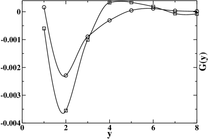
Figure 3: Transverse Green’s function $G(y)$ for $t_{d}=0$ (circles), $t_{d}=0.1$ (squares).

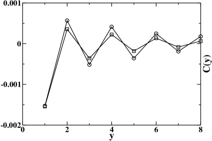
Figure 4: Transverse spin-spin correlation $C(y)$ for $t_{d}=0$ (circles), $t_{d}=0.1$ (squares).

The 1D interacting electron gas is now fairly well understood. bourbonnais There is no phase with long range order. There are essentially four regions in the phase diagram, characterized by the dominant correlations i.e., SDW, charge density wave (CDW), singlet superconductivity (SS) and triplet superconductivity (TS). The essential question is whether the interchain hopping will simply freeze the dominant 1D fluctuation into long-range order (LRO) or create new 2D physics. The estimated values of $U$ and $V$ for the Bechgaard salts suggest that they are in the SDW region in their 1D regime. This suggests that superconductivity in these materials is a 2D phenomenon. Interchain pair tunneling was suggested soon after the discovery of superconductivity in an organic compound.jerome-shulz Emery argued instead that a mechanism similar to the Kohn-Luttinger mechanism might be responsible for superconductivity in the organic materials. When $t_{\perp}$ is turned on, pairing can arise from exchange of short-range SDW fluctuations. The reason is that the oscillating SDW susceptibility at $Q=(2k_{F},k_{\perp})$ would have an attractive region if $k_{\perp}\neq 0$. In particular if $k_{\perp}=\pi$ as I found, then the interaction would be attractive between particles in neighboring chains. In this study, I will restrain myself to the study of interchain pair tunneling. I was unable to compute correlation functions of pairs in which each electron belongs to a different chain. The reason is that in the DMRG method, for the correlation functions to be accurate, at least two different blocks should be involved. This means that for pair correlation for which each electron of the pair is on a different chain, at least four blocks are needed. However, the introduction of four blocks in the second step of the TSDMRG leads to a prohibitive CPU time.

With the hope of frustrating an SDW ordering which is usually expected, I will add an extra terms to model (1) . These are the diagonal interchain hopping,

$$H_{d}=-t_{d}\sum_{i,l,\sigma}(c_{i,l,\sigma}^{\dagger}c_{i+1,l+1,\sigma}+$$

$$h.c)+(c_{i+1,l,\sigma}^{\dagger}c_{i,l-1,\sigma}+h.c),$$ (11)

and the next-nearrest neighbor interchain hopping,

$$H^{\prime}_{\perp}=-t^{\prime}_{\perp}\sum_{i,l,\sigma}(c_{i,l,\sigma}^{\dagger}c_{i,l+2,\sigma}+h.c).$$

I will also add the interchain Coulomb interaction,

$$H_{V}=V_{\perp}\sum_{i,l,\sigma}n_{i,l,\sigma}.n_{i,l+1,\sigma}$$ (12)

I set $t_{\perp}=0.2$, $ms_{1}=256$, $ms_{2}=128$, and $(L\times(L+1)=16\times 17$. A second set of calculations with $t_{\perp}=0.15$, same values of $ms_{1}$ and $ms_{2}$, and $(L\times(L+1)=24\times 25$ lead to the same conclusions. Therefore, they will not be shown here. In order to analyze the physics induced by the transverse couplings, I compute the following interchain correlations: the transverse single-particle Green’s function, shown in Fig.3,

$$G(y)=\langle c_{L/2,L/2+y}c_{L/2,L/2+1}^{\dagger}\rangle,$$ (13)

the transverse spin-spin correlation function, shown in Fig.4,

$$C(y)=\frac{1}{3}\langle{\bf S}_{L/2,L/2+y}{\bf S}_{L/2,L/2+1}\rangle,$$ (14)

the transverse local pairs singlet superconductive correlation, shown in Fig.5,

$$SS(y)=\langle\Sigma_{L/2,L/2+y}\Sigma_{L/2,L/2+1}^{\dagger}\rangle,$$ (15)

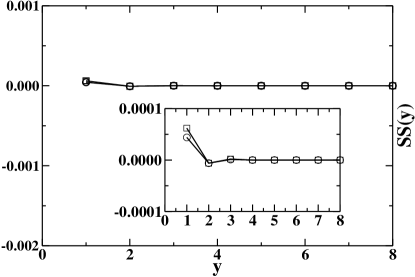
Figure 5: Transverse local singlet correlation $SS(y)$ for $t_{d}=0$ (circles), $t_{d}=0.1$ (squares).

where

$$\Sigma_{i,l}=c_{i,l\uparrow}c_{i,l\downarrow},$$ (16)

the transverse triplet superconductive correlation, shown in Fig.6,

$$ST(y)=2\langle\Theta_{L/2,L/2+y}\Theta_{L/2,L/2+1}^{\dagger}\rangle,$$ (17)

where

$$\Theta_{i,l}=\frac{1}{\sqrt{2}}(c_{i,l\uparrow}c_{i+1,l\downarrow}+c_{i,l\downarrow}c_{i+1,l\uparrow}),$$ (18)

and the transverse non-local singlet pair superconductive correlation function, shown in Fig.7,

$$SD(y)=2\langle\Delta_{L/2,L/2+y}\Delta_{L/2,L/2+1}^{\dagger}\rangle,$$ (19)

where

$$\Delta_{i,l}=\frac{1}{\sqrt{2}}(c_{i,l\uparrow}c_{i+1,l\downarrow}-c_{i,l\downarrow}c_{i+1,l\uparrow}).$$ (20)

IV.1 Strong-coupling regime

Let us first consider, the regime $U\gtrsim 4$, I choose for instance $U=4$, $V=0.85$, $\mu=0$, and $t_{d}=t^{\prime}_{\perp}=V_{\perp}=0$; besides single-particle hopping, $t_{\perp}$ also generates two-particle hopping both in the particle-hole and particle-particle channels. These two-particle correlation functions are roughly given by the average values $t_{\perp}^{2}\langle c_{i,l\sigma}^{\dagger}c_{i,l-\sigma}c_{i,l+j-\sigma}^{\dagger}c_{i,l+j\sigma}\rangle$ and $t_{\perp}^{2}\langle c_{i,l\sigma}^{\dagger}c_{i,l-\sigma}^{\dagger}c_{i,l+j\sigma}c_{i,l+j-\sigma}\rangle$ for an on-site pair created at $(i,l)$ and then destroyed at $(i,l+j)$. It is expected that the dominant two-particle correlation are SDW with $k_{\perp}=\pi$. This is seen in Fig.(4-7). The transverse pairing correlations are all found to be small with respect to $C(y)$. Among the pairing correlations, $SS(y)$ decays faster then $ST(y)$ and $SD(y)$. These results are consistent with the view that the role of $t_{\perp}$ is to freeze the dominant 1D correlations into LRO.

When $t_{d}\neq 0$, it is expected that for a strong enough $t_{d}$, the magnetic order will vanish because of the frustration induced by $t_{d}$. A simple argument is that $t_{d}$ induces an AFM exchange between next-nearest neigbhors on chains $l$ and $l+1$ which compete with the AFM exchange between nearest neigbhors. The hope is that there could be a region of the phase diagram where superconductivity could ultimately win either by pair tunneling between the chains or by the Emery’s mechanism. However, in Fig.(4-7) it can be seen that, while $t_{d}$ slightly reduces $C(y)$, the dominant correlations are still SDW even for a strong $t_{d}/t_{\perp}=0.5$. $SS(y),~{}ST(y)$ and $SD(y)$ are barely affected by $t_{d}$. The fact that $t_{d}$ does not strongly affect the SDW order can be understood in the light of recent study of coupled $t-J$ chains moukouri-TSDMRG2 . It was shown that the frustration strongly suppresses magnetic LRO only close to half-filling. For large dopings, two neighboring spins in a chain do not always points to opposite direction as the consequence, $t_{d}$ does not necessarily frustrate the magnetic order. This is illustrated in a simple sketch in Fig.(8). $t_{d}$ could even enhance it as seen in the study of $t-J$ chains. In Fig.3, it can be seen that $t_{d}$ enhances $G(y)$. This enhancement, together with the decrease of $C(y)$, suggests a possible widening of an eventual Fermi liquid region at finite T above the ordered phase. When $t_{\perp}\neq 0$, I also found (not shown) that magnetic correlation are not effectively suppressed even when $t^{\prime}_{\perp}=t_{\perp}/2$. For this value, it would be expected that the ratio of the effective exchange term generated by $t^{\prime}_{\perp}$ to that generated by $t_{\perp}$ is about one quarter. In the frustrated $J_{1}-J_{2}$ spin chain, a spin gap opens around this ratio. This simple picture does not seem to work here.

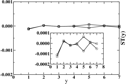
Figure 6: Transverse triplet superconductive correlation $ST(y)$ for $t_{d}=0$ (circles), $t_{d}=0.1$ (squares).

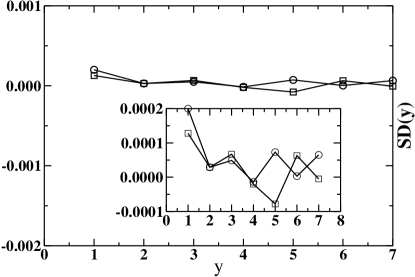
Figure 7: Transverse singlet non-local superconductive correlation $SD(y)$ for $t_{d}=0$ (circles), $t_{d}=0.1$ (squares).

Figure 8: sketch of the spin texture (arrows) in two consecutive chains in an SDW. The bold horizontal lines represent the chains. The full diagonal lines show bonds for which $t_{d}$ tends to increase the SDW order. The diagonal dotted lines show bonds for which $t_{d}$ frustrates the magnetic order.

IV.2 Weak-coupling regime

I now turn in to the regime where $U\lesssim 4$. I set $U=2$, $V=0$, $\mu=-0.9271$, $t_{\perp}=0.2$, $t_{d}=0$, and $V_{\perp}=0.4$, where $V_{\perp}$ is the interchain Coulomb interaction between nearest neighbors. It can be seen in Fig.9 that $C(y)$ is now strongly reduced with respect to its strong coupling values. It is already within our numerical error for the next-nearest neighbor in the transverse direction. This is an indication that the ground state is probably not an SDW. It is to be noted that this occurs even in the absence of $t_{d}$ or $t^{\prime}_{\perp}$. This seems to be at variance with the RG analysis which requires $t^{\prime}_{\perp}$ to destroy the magnetic order. A possible explanation of this is that at half-filling the perfect nesting occurs at the wave vector $Q=(\pi,\pi)$ for the spectrum of equation (9). Away from half-filling the nesting is no longer perfect this leads to the reduction of magnetic correlations. The first correction to the nesting is an effective frustration term which is roughly $t_{\perp}^{2}cos2k_{\perp}$. This expression is identical to a term that could be generated by an explicit frustration $t^{\prime}_{\perp}=t_{\perp}^{2}$. The discrepancy between the TSDMRG and the RG results could be that this nesting deviation is underevaluated in the RG analysis. This mechanism cannot be invoked in the strong coupling regime where band effects are small.

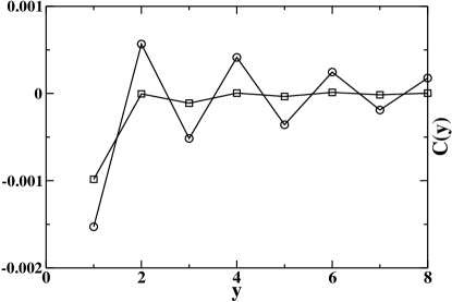
Figure 9: Transverse spin-spin correlation $C(y)$ for $U=4$ (circles), $U=2$ and $V_{\perp}=0.4$ (squares).

The suppression of magnetism is concommitant to a strong enhancement of the singlet pairing correlations as seen in Fig. 11. Triplet correlations, shown in Fig. 10, remain very small. However, while it is clear from the behavior of $C(y)$ that the ground state is non magnetic. This result strongly suggests that the ground state is a superconductor in this regime. A finite size analysis is, however, necessary to conclude whether this persists to the thermodynamic limit. I cannot rule out the possibility of a Fermi liquid ground state, which is implied by strong single particle correlations.

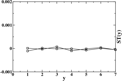
Figure 10: Transverse triplet superconductive correlation $ST(y)$ for $U=4$ (circles), $U=2$ and $V_{\perp}=0.4$ (squares).

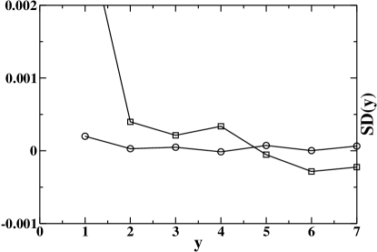
Figure 11: Transverse singlet non-local superconductive correlation $SD(y)$ for $U=4$ (circles), $U=2$ and $V_{\perp}=0.4$ (squares).

V Conclusion

In this paper, I have presented a TSDMRG study of the competition between magnetism and superconductivity in an anisotropic Hubbard model. I have analyzed the effect of the interchain hopping in the strong and weak $U$ regimes. In the strong-coupling regime, the results are consistent with earlier predictions that the role of $t_{\perp}$ is to freeze the dominant 1D SDW correlations into a 2D ordered state. But at variance with analytical predictions, this is only true in the strong $U$ regime. In this regime, I find that even the introduction of frustration does not disrupt the SDW order which remain robust up to large values of the frustration. In the weak coupling regime singlet pair correlations are dominant. The ground state seems to be a superconductor. This behavior is somewhat in agreement with experiments in the Bechgaard or Fabre salts. The phase diagram is dominated by magnetism at low pressure (strong U) and by superconductivity at high pressure (weak U). Because of experimental relevance, I restricted myself to the competion between magnetism and superconductivity. I did not analyze CDW correlations. These are likely to be important given that I applied open boundary conditions which are known to generate Friedel oscillations wsa that very decay slowly from the boundaries. They may also genuinely generated by $V_{\perp}$, leading to a CDW ground state instead of a superconductor.

- (1) C. Bourbonnais and D. Jérome in ”Advance in Synthetic Metals” Eds. P. Bernier, S. Lefrant and G. Bidan (Elsevier, New York), 206 (1999).
- (2) J.W. Allen, Sol. St. Comm. 123, 469 (2002).
- (3) C. Bourbonnais and L.G. Caron, Int. J. Mod. Phys. B 5, 1033 (1991).
- (4) T. Giamarchi in ”Quantum Physics in One Dimension”, Clarendon Press Eds, P. 254-269 (2004).
- (5) S. Biermann, A. Georges, A. Lichtenstein, and T. Giamarchi, Phys. Rev. Lett. 87, 276405 (2001).
- (6) S.R. White, D.J. Scalapino, R.L. Sugar, E.Y. Loh, J.E. Gubernatis, and R.T. Scalettar, Phys. Rev. B 40, 506 (1989).
- (7) S. Moukouri, Phys. Rev. B 70, 014403 (2004).
- (8) S. Moukouri, J. Stat. Mech. P02002 (2006)
- (9) S.R. White, Phys. Rev. Lett. 69, 2863 (1992). Phys. Rev. B 48, 10 345 (1993).
- (10) S.R. White, Phys. Rev. B 72, 180403 (2005).
- (11) V.J. Emery, Synthetic Metals, 13, 21 (1986).
- (12) I.J. Lee et al., Phys. Rev. Lett. 88, 017004 (2002).
- (13) N. Dupuis, C. Bourbonnais and J.C. Nickel, cond-mat/0510544.
- (14) D. Jerome and H.J. Schulz, Adv. Phys. 31, 299 (1982).
- (15) D. Jerome, Chem. Rev. 104, 5565 (2004). D. Jerome and C.R. Pasquier, in Superconductors, edited by A.V. Narlikar (Springer Verlag, Berlin, 2005).
- (16) Y. Shinagawa, et al., cond-mat/0701566 (2007).
- (17) Y. Tanaka and K. Kuroki, Phys. Rev. B 70, 060502 (2004).
- (18) Mahito Kohmoto and Masatoshi Sato, cond-mat/0001331 (2000).
- (19) I.J. Lee, M.J. Naughton, P.M. Chaikin, Physica B 294-295, 413 (2001).
- (20) S. R. White, Ian Affleck, and D. J. Scalapino, Phys. Rev. B 65, 165122 (2002).