Chromospheric Cloud-Model Inversion Techniques

Abstract

Spectral inversion techniques based on the cloud model are extremely useful for the study of properties and dynamics of various chromospheric cloud-like structures. Several inversion techniques are reviewed based on simple (constant source function) and more elaborated cloud models, as well as on grids of synthetic line profiles produced for a wide range of physical parameters by different NLTE codes. Several examples are shown of how such techniques can be used in different chromospheric lines, for the study of structures of the quiet chromosphere, such as mottles/spicules, as well as for active region structures such as fibrils, arch filament systems (AFS), filaments and flares.

National Observatory of Athens, Institute for Space Applications and Remote Sensing, Greece

1 Introduction

Observed intensity line profiles are a function of several parameters describing the three-dimensional solar atmosphere, such as chemical abundance, density, temperature, velocity, magnetic field, microturbulence etc (which one would like to determine), as well as of wavelength, space (solar coordinates) and time. However, due to the large number of parameters that an observed profile depends on, as well as data noise, model atmospheres have to be assumed in order to restrict the number of these unknown parameters. The term “inversion techniques” refers to the procedures used for inferring these model parameters from observed profiles. We refer the reader to Mein (2000) for an extended overview of inversion techniques. In this paper, we will review only a class of such inversion techniques known in the solar community as “cloud models”.

Cloud models refer to models describing the transfer of radiation through structures located higher up from the solar photosphere, which represents the solar surface, resembling clouds on earth’s sky (see Fig. 1). Such cloud-like structures, when observed from above, would seem to mostly absorb the radiation coming from below, an absorption which mostly depends on the optical thickness of the cloud, that is the “transparency” of the cloud to the incident radiation and also on the physical parameters that describe it. The possibility of observed emission from such structures cannot, of course, be excluded when the radiation produced by the cloud-like structure is higher than the absorbed one. The aforementioned processes are described by the radiative transfer equation

$$I(\Delta\lambda)=I_{\rm 0}(\Delta\lambda)~{}{\rm e}^{-\tau(\Delta\lambda)}+\int_{0}^{\tau(\Delta\lambda)}S_{t}~{}{\rm e}^{-t(\Delta\lambda)}~{}{\rm d}t\,,$$ (1)

where $I(\Delta\lambda)$ is the observed intensity, $I_{\rm 0}(\Delta\lambda)$ is the reference profile emitted by the background (the incident radiation to the cloud from below), $\tau(\Delta\lambda)$ is the optical thickness and $S$ the source function which is a function of optical depth along the cloud. The first term of the right hand part of the equation represents the absorption of the incident radiation by the cloud, while the second term represents emission by the cloud itself.

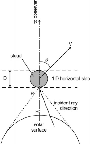
Figure 1.: Geometry of the cloud model. $D$ is the geometrical thickness of the cloud at height $H$ above the solar surface and $V$ its velocity. From Heinzel et al. (1999).

The simple cloud model method introduced by Beckers (1964) arose from the need to solve fast the radiation transfer equation and deduce the physical parameters that describe the observed structure. Beckers assumed that a) the structure is fully separated from the underlying chromosphere, b) the source function, radial velocity, Doppler width and the absorption coefficient are constant along the line-of-sight (hereafter LOS) and c) the background intensity is the same below the structure and the surrounding atmosphere; hence it can be extrapolated from a neighboring to the structure under study region. Under the above assumptions the radiative transfer equation is simplified to

$$I(\Delta\lambda)=I_{0}(\Delta\lambda)~{}{\rm e}^{-\tau(\Delta\lambda)}+S(1-{\rm e}^{-\tau(\Delta\lambda)})$$ (2)

and can be rewritten as

$$C(\Delta\lambda)=\displaystyle\frac{I(\Delta\lambda)-I_{0}(\Delta\lambda)}{I_{0}(\Delta\lambda)}\\ =\displaystyle\left(\frac{S}{I_{0}(\Delta\lambda)}-1\right)(1-{\rm e}^{-\tau(\Delta\lambda)})\,,$$

where $C(\Delta\lambda)$ defines the contrast profile. A Gaussian wavelength dependence is usually assumed for the optical depth as follows

$$\tau(\Delta\lambda)=\tau_{0}~{}{\rm e}^{-\displaystyle\left({\frac{\Delta\lambda-\Delta\lambda_{I}}{\Delta\lambda_{\rm D}}}\right)^{2}}\,,$$ (3)

where $\tau_{0}$ is the line center optical thickness, $\Delta\lambda_{I}=\lambda_{0}v/c$ is the Doppler shift with $\lambda_{0}$ being the line center wavelength, $c$ the speed of light and $\Delta\lambda_{\rm D}$ is the Doppler width. The latter depends on temperature $T$ and microturbulent velocity $\xi_{\rm t}$ through the relationship

$$\Delta\lambda_{\rm D}=\frac{\lambda_{0}}{c}\sqrt{\xi^{2}_{\rm t}+\frac{2kT}{m}}\,,$$ (4)

where $m$ is the atom rest mass. Other wavelength dependent profiles than the Gaussian one can also be assumed for the optical depth, e.g., a Voigt profile (Tsiropoula et al. 1999).

The four adjustable parameters of the model are the source function $S$, the Doppler width $\Delta\lambda_{\rm D}$, the optical thickness $\tau_{0}$ and the LOS velocity $v$. All these parameters are assumed to be constant through the structure. There are some crucial assumptions concerning Beckers’ cloud model (hereafter BCM):

• the uniform background radiation assumption, which is not always true especially for cloud-like structures that do not reside above quiet Sun regions. Moreover, the background radiation plays an important role in the correct quantitative determination of the physical parameters.

• the neglect of incident radiation, the effects of which are of course not directly considered in BCM, but does play an important role in non-Local Thermodynamic Equilibrium (hereafter NLTE) modeling, since it determines the radiation field within the structure, that is the excitation and ionization conditions and hence the source function.

• the constant source function assumption which is not realistic especially in the optically thick case or not valid in the presence of large velocity gradients.

However, the cloud model works quite well for a large number of optically thin structures and can provide useful, reasonable estimates for the physical parameters that describe them. We refer the reader to Alissandrakis et al. (1990) for a detailed discussion on the validity conditions of BCM for different types of contrast profiles.

2 Cloud Model Variants

Since the introduction of the BCM method several improvements have been suggested in the literature. When looking at the radiative transfer equation (Eq. 1), it is obvious that all efforts concentrate on a better description of the source function $S$ which in BCM is considered to be constant. In the following subsections some of these suggested improvements are described.

2.1 Variable source function

Mein et al. (1996a) considered a source function that is a function of optical depth and is approximated by a second-order polynomial

$$S_{\rm t}=S_{0}+S_{\rm 1}\frac{\tau_{0}}{\tau_{\rm 0,max}}+S_{2}\left(\frac{\tau_{0}}{\tau_{\rm 0,max}}\right)^{2}$$ (5)

with the optical depth at the center of the line $\tau_{0}$ taking values between 0 and the total optical thickness at line center $\tau_{\rm 0,max}$, while $S_{0}$, $S_{1}$ and $S_{2}$ are functions of $\tau_{\rm 0,max}$. This formulation was further improved by Heinzel et al. (1999), who included also the effect of cloud motion by assuming that $S_{0}$, $S_{1}$ and $S_{2}$ are now not only functions of $\tau_{\rm 0,max}$, but also depend on the velocity $v$ of the structure.

Tsiropoula et al. (1999) assumed the parabolic formula

$$S_{t}=S_{0}\left(1+\alpha\left(t-\frac{\tau_{\rm 0}}{2}\right)^{2}\right)$$ (6)

as an initial condition for the variation of the source function with optical depth, where $S_{0}$ is the source function at the middle of the structure, $\tau_{0}$ the optical depth at line center, and $\alpha$ a constant expressing the variation of the source function. However, their final results on the dependence of the source on optical depth were in good agreement with the results of Mein et al. (1996a).

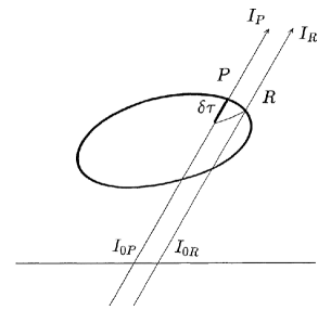
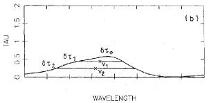
Figure 2.: Left: Geometry of the cloud model in the case of first-order differential cloud model. From Heinzel et al. (1992). Right: The “3-optical depths” procedure for solving the differential cloud model case which is described in Sect. 3.5 (from Mein & Mein (1988)).

2.2 Differential cloud models

First and second order differential cloud models (hereafter DCM1 and DCM2) were introduced by Mein & Mein (1988) to account for fast mass flows observed on the disc, where BCM is not valid due to fluctuations of the background and strong velocity gradients along the LOS. DCM1 assumes that the source function $S$, temperature $T$ and velocity $v$ are constant within a small volume contained between two close lines of sight $P$ and $R$ (see Fig. 2, left panel). If we assume that the variation of the background profile is negligible ($I_{\rm 0P}\simeq I_{\rm 0R}$) for such close points then the differential cloud contrast profile can be written as

$$C(P,R,\lambda)=\frac{I_{P}(\lambda)-I_{\rm R}(\lambda)}{I_{R}(\lambda)}=\left(\frac{S}{I_{\rm R}(\lambda)}-1\right)(1-{\rm e}^{-\delta\tau(\lambda)})$$ (7)

with

$$\delta\tau(\lambda)=\delta\tau_{0}~{}{\rm e}^{-\displaystyle\left(\frac{\lambda-\lambda_{0}-v\lambda_{\rm 0}/c}{\Delta\lambda_{\rm D}}\right)^{2}}\,,$$ (8)

where $\Delta\lambda_{\rm D}$ is the Doppler width. The zero velocity reference wavelength $\lambda_{0}$ is obtained by averaging over the whole field of view. DCM1 is a method for suppressing the use of the background radiation. If velocity shears are present between neighboring LOS then DCM2 can be used instead which requires the use of three neighboring LOS. We refer the reader to Mein & Mein (1988) for the precise formulation of DCM2 and to Table 1 of the same paper which summarizes the validity conditions, constrains and results of the two models in comparison to the classical BCM.

2.3 Multi-cloud models

The multi-cloud model (Gu et al. 1992, 1996) – hereafter MCM – was introduced for the study of asymmetric, non-Gaussian profiles, such as line profiles of post-flare loops, prominences and surges and was based on the BCM and DCMs models. These asymmetric line profiles are assumed to be the result of overlapping of several symmetric Gaussian profiles along the LOS, formed in small radiative elements (clouds) which have a) different or identical physical properties and b) a source function and velocity independent of depth. The profile asymmetry mostly results from the relative Doppler shifts of the different clouds. The total intensity $I_{\lambda}$ emitted by $m$ clouds is then given by the relation

$$I_{\lambda}=I_{0,\lambda}\,{\rm e}^{-\tau_{\lambda}}+\sum_{j=1}^{m}S_{j}(1-{\rm e}^{-\tau_{\lambda,j}})\exp\left(-\sum_{i=0}^{j-1}\tau_{\lambda,i}\right)\,,$$ (9)

where $\tau_{\lambda,0}=0$, $I_{0,\lambda}$ is the background intensity, $\tau_{\lambda}=\sum_{j=1}^{m}\tau_{\lambda,j}$ is the total optical depth of the $m$ clouds and

$$\tau_{\lambda,j}=\tau_{0,j}~{}{\rm e}^{-\displaystyle\left(\frac{\lambda-\lambda_{0}-\Delta\lambda_{0,j}}{\Delta\lambda_{{\rm D},j}}\right)^{2}}$$ (10)

$\Delta\lambda_{0,j}=\lambda_{0}v_{j}/c$, $S_{j}$, $\tau_{0,j}$, $v_{j}$, $\Delta\lambda_{{\rm D},j}$ are respectively the optical depth, Doppler shift, source function, line-center thickness, velocity and Doppler width of the $j^{\rm th}$ cloud.

A somewhat similar in philosophy, two-cloud model method was used by Heinzel & Schmieder (1994) in their study of black and white mottles. It was assumed that the LOS intersects two mottles treated as two different clouds $c1$ and $c2$ with optical depths $\tau_{1}$ and $\tau_{2}$ respectively. Hence the emerging intensity from the lower mottle $I_{1}$ is assumed to be the background incident intensity for the second upper mottle. Then, the equations describing the radiation transfer through the two mottles are

$$I_{2}(\Delta\lambda) = I_{\rm 1}~{}{\rm e}^{-\tau_{2}(\Delta\lambda)}+I_{c2}(\Delta\lambda)$$

$$I_{1}(\Delta\lambda) = I_{\rm 0}~{}{\rm e}^{-\tau_{1}(\Delta\lambda)}+I_{c1}(\Delta\lambda)\,,$$ (11)

where $I_{0}$ is the background chromospheric intensity and $I_{c1}$, $I_{c2}$ the intensity emitted by the two clouds respectively. The novelty of the method is that for the emitted by the clouds intensity, a grid of 140 NLTE models was used which was computed for prominence-like structures by Gouttebroze et al. (1993). So this method is a combination of MCM with NLTE source function calculations which will be further discussed in Section 2.6.

2.4 The Doppler signal method

The Doppler signal method (Georgakilas et al. 1990; Tsiropoula 2000) can be used when filtergrams at two wavelengths $-\Delta\lambda$ and $+\Delta\lambda$ (blue and red side of the line) are available and a fast determination of mass motions is needed. Then the Doppler signal $DS$ can be defined from the BCM equations as

$$DS=\frac{\Delta I}{\sum I-2I_{0}}=\frac{{\rm e}^{-\tau^{+}}-{\rm e}^{-\tau^{-}}}{2-{\rm e}^{-\tau^{+}}-{\rm e}^{-\tau^{-}}}\,,$$ (12)

where $\Delta I=I(-\Delta\lambda)-I(+\Delta\lambda)$, $\sum I=I(-\Delta\lambda)+I(+\Delta\lambda)$ and $\tau^{\pm}=\tau(\pm\Delta\lambda)$. The Doppler signal $DS$ has the same sign as velocity and can be used for a qualitative description of the velocity field. The left hand side of the above equation can be determined by the observations while the right hand clearly does not depend on the source function. Quantitative values for the velocity can be obtained when $\tau_{0}<1$; then the Doppler signal equation reduces to

$$DS=\frac{\tau^{-}-\tau^{+}}{\tau^{-}+\tau^{+}}$$ (13)

and the velocity $v$ – once $DS$ is calculated from the observations and a value of the Doppler width $\Delta\lambda_{\rm D}$ is obtained from the literature or assumed – is given by the equation

$$v=\displaystyle\frac{\Delta\lambda_{\rm D}^{2}}{4\Delta\lambda}\frac{c}{\lambda}\ln\left(\frac{1+DS}{1-DS}\right)\,.$$ (14)

2.5 Avoiding the background profile

Liu & Ding (2001) in order to avoid the use of the background profile needed in BCM assumed that it is symmetric, that is $I_{0}(\Delta\lambda)=I_{0}(-\Delta\lambda)$. Then it can easily be shown that we can obtain the relationship

$$\Delta I(\Delta\lambda)=I(\Delta\lambda)-I(-\Delta\lambda)=[I(\Delta\lambda)-S][1-{\rm e}^{\tau(\Delta\lambda)-\tau(-\Delta\lambda)}]\,,$$ (15)

which does not require the use of the background for the derivation of the physical parameters.

2.6 NLTE methods

As Eq. 1 shows, in the general case, the source function $S$ within a cloud-like structure is not constant, but usually depends on optical depth. In order to calculate this dependence, the NLTE radiative transfer problem within the structure has to be solved, taking into account all excitation and ionization conditions within the structure. Several efforts have been undertaken in the past for such NLTE calculations, usually for the case of filaments or prominences. Such NLTE calculations started from the one-dimensional regime, where the cloud-like structure is approximated by an infinite one-dimensional slab (see Fig. 1) or a cylinder. We refer the reader to the works of Heasley et al. (1974), Heasley & Mihalas (1976), Heasley & Milkey (1976), Mozozhenko (1978), Fontenla & Rovira (1985), Heinzel et al. (1987), Gouttebroze et al. (1993), Heinzel (1995), Gouttebroze (2004) for an overview of such one-dimensional NLTE models. The philosophy of two-dimensional NLTE models is similar to the one-dimensional models, but now the cloud-like structure is replaced by a two-dimensional slab or cylinder which is infinite in the third dimension, allowing both vertical, as well as horizontal radiation transport (see Fig. 3). Furthermore, the incident radiation is treated as anisotropic and comes now not only from below, but also from the sides of the structure. We refer the reader to the works of Mihalas et al. (1978), Vial (1982), Paletou et al. (1993), Auer & Paletou (1994), Heinzel & Anzer (2001), Gouttebroze (2005) for an overview of such two-dimensional NLTE models.

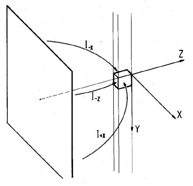
Figure 3.: Geometry of a two-dimensional cloud model slab. The incident radiation comes not only from below, but also from the sides of the structure. From Vial (1982).

A general recipe for such NLTE models, which is modified according to the specific needs, i.e. the line profile used and the structure observed, has as follows:

• The cloud-like structure is assumed to be a 1-D or 2-D slab or cylinder at a height $H$ above the photosphere. This slab/cylinder can be considered to be either isothermal (e.g., Heinzel 1995) or isothermal and isobaric (e.g., Paletou et al. 1993).

• The incident radiation comes in the case of 1-D models only from below and in the case of 2-D models also from the sides and determines the radiation field within the structure, that is all excitation and ionization conditions.

• A multi-level atom plus continuum is assumed. The larger the number of atomic levels used, the more computationally demanding the method is. Complete or partial redistribution effects (CRD or PRD) are also assumed depending on the formation properties of the line. Methods with CRD are computationally much faster so sometimes CRD is used but with simulated PRD effects taken into account (e.g., Heinzel 1995).

• Some physical parameters are assigned to the slab/cylinder, like temperature $T$, bulk velocity $v$, geometrical thickness $Z$, electronic density $N_{\rm e}$ or pressure $p$. Calculations with electronic density are usually faster than calculations with pressure.

• The radiative transfer statistical equilibrium equations are numerically solved and the population levels are found and hence the source function as a function of optical depth for a set of selected physical parameters.

Once the source function $S$ is obtained as a function of optical depth, Eq. 1 can be solved in order to calculate the emerging observed profile from the structure which is going to be compared to the observed one.

3 Solving the Cloud Model Equations

In the following subsections some of the methods used to solve the cloud model equations are reviewed. We remind the reader that whenever the background profile is needed, either the average profile of a quiet Sun region is taken or the average profile of a region close to the structure under study.

3.1 Solving the constant-$S$ case with the “5-point” method

Mein et al. (1996a) introduced the “5-point method” for solving the BCM equation with constant $S$. According to this method five intensities of the observed and the background profile at wavelengths $\lambda_{1}$, $\lambda_{2}$ (blue wing of the observed profile), $\lambda_{3}$, $\lambda_{4}$ (red wing of the the observed profile) and the line-center wavelength $\lambda_{0}$ are used for solving Eqs. 1 and 3. It is an iterative method that works as follows:

• The line-center wavelength $\lambda_{0}$ profile and background intensities are used for calculating $S$, where $\tau_{0}$, $\Delta\lambda_{\rm D}$ and $v$ are determined in a previous iteration. At the first step of the iteration some values can be assumed and $S$ can be taken as equal to zero.

• Profile and background intensities at wavelengths $\lambda_{\rm 1}$ and $\lambda_{3}$ are used for calculating a new $\tau_{\rm 0}$.

• Afterwards a new $\Delta\lambda_{\rm D}$ is calculated using the other two remaining wavelengths $\lambda_{2}$ and $\lambda_{4}$.

• Finally a new velocity is calculated from wavelengths $\lambda_{1}$, $\lambda_{2}$, $\lambda_{3}$, and $\lambda_{4}$ and then a reconstructed profile obtained using the derived parameters which is compared to the observed one. If any of the departures between the reconstructed and the observed profile is higher than an assumed small threshold value (i.e. 10^-4) then the aforementioned procedure is repeated until convergence is achieved. If no convergence is gained after a certain number of iterations then it is assumed that no solution exists.

We refer the reader to Mein et al. (1996a) for a detailed description of the analytical equations described above.

3.2 Solving the constant-$S$ case with an iterative least-square fit

This method which was used by Alissandrakis et al. (1990) and further described in Tsiropoula et al. (1999) and Tziotziou et al. (2003) fits the observed contrast profile with a curve that results from an iterative least-square procedure for non-linear functions which is repeated until the departures between computed and observed profiles are minimized. The coefficients of the fitted curve are functions of the free parameters of the cloud model. At the beginning of the iteration procedure initial values have to be assumed for the free parameters and especially for the source function $S$ which is usually estimated from some empirical approximate expressions that relate it to the line-center contrast. This method is very accurate and usually converges within a few iterations. The more observed wavelengths used within the profile, the better the determination of the ohysical parameters is. However, as Tziotziou et al. (2003) have reported, the velocity calculation can overshoot producing very high values, if the wings of the profile are not sufficiently covered by observed wavelengths. The suggested way to overcome the problem is to artificially add two extra contrast points near the continuum of the observed profile where the contrast should be in theory equal to zero.

This iterative method can also be successfully used not only in the case of a constant source function $S$, but also for cases with a prescribed expression for the source function, such as the parabolic expression of Eq. 6 used by Tsiropoula et al. (1999).

3.3 Solving the constant-$S$ case with a constrained nonlinear least-square fitting technique

The constrained nonlinear least-square fitting technique, used by Chae et al. (2006) for the inversion of a filament with BCM, was introduced by Chae et al. (1998). According to the method a) expectation values $p_{i}^{e}$ of the $i$th free parameters, b) their uncertainties $\varepsilon_{i}$, as well as c) the data to fit are provided ($M$ wavelengths along the profile) and then a set of $N$ free parameters ${\bf p}=(p_{0},p_{1},...p_{N-1})$ are sought, i.e. ${\bf p}=(S,\tau_{0},\lambda_{0},\Delta\lambda_{\rm D})$, that minimize the function

$$H({\bf p})=\sum_{j=0}^{M-1}\left(\frac{C^{\rm obs}_{j}-C^{\rm mod}_{j}({\bf p})}{\sigma_{j}}\right)^{2}+\sum_{i=0}^{N-1}\left(\frac{p_{i}-p^{e}_{i}}{\varepsilon_{i}}\right)^{2}\,,$$ (16)

where $C^{\rm obs}_{j}$ and $C^{\rm mod}_{j}$ are respectively the observed and calculated with the expectation values contrasts and $\sigma_{j}$ the noise in the data. The first term of the sum $H$ represents the data $\chi^{2}$, while the second term the expectation $\chi^{2}$ which regularizes the solution by constraining the probable range of free parameters. For very small values of $\varepsilon_{i}$ the solution will not be much constrained by the data and will be close to the chosen set of expectation values $p_{i}^{e}$, while for large values of $\varepsilon_{i}$ it will be mostly constrained by the data and not by the expectation values. We refer the reader to Chae et al. (2006) for a detailed discussion of the effects of constrained fitting.

3.4 Solving the variable-$S$ case

Apart from the iterative least-square procedure described above which can be used when the source function varies in a prescribed way, Mein et al. (1996a) have introduced also the “4-point method” for solving the case of a source function that is described by the second order polynomial of Eq. 5. According to the method an intensity $I^{\prime}(\Delta\lambda)$ can be defined as follows

$$I^{\prime}(\Delta\lambda) = I(\Delta\lambda)-\frac{1-[\tau(\Delta\lambda)+1]~{}{\rm e}^{-\tau(\Delta\lambda)}}{\tau(\Delta\lambda)}~{}S_{1}+$$ (17)

$$\frac{2-[\tau^{2}(\Delta\lambda)+2\tau(\Delta\lambda)+2]~{}{\rm e}^{-\tau(\Delta\lambda)}}{\tau^{2}(\Delta\lambda)}~{}S_{2}$$

and then the radiative transfer equation reduces to

$$I^{\prime}(\Delta\lambda)=S_{0}+(I_{0}-S_{\rm 0})~{}{\rm e}^{-\tau(\Delta\lambda)}\,.$$ (18)

This equation can be solved now using the iteration procedure described in Sect. 3.1, with the modification that $I(\Delta\lambda)$ is now replaced by $I^{\prime}(\Delta\lambda)$ and that the source function calculation in the first step is replaced by the assumed theoretical relation for $S$ given by Eq. 5.

3.5 Solving the DCM cases

A method for solving the differential cloud model cases is the “3-optical depths” procedure introduced by Mein & Mein (1988). According to this procedure:

• the zero velocity reference is obtained from the average profile over the whole field of view;

• a value $S$ is assumed between zero and the line-center intensity (in principle it could even work also for emitting clouds) and a function $\delta\tau(\lambda)$ is derived from Eq. 7. The latter is characterized by the maximum value $\delta\tau_{0}$ and $\delta\tau_{1}$, and the values $\delta\tau_{2}$ (see right panel of Fig. 2) which correspond to the half widths $\Delta\lambda_{1}$ and $\Delta\lambda_{2}$ respectively and are given by the following relations

  $$\delta\tau_{1} = \delta\tau_{\rm 0}~{}{\rm e}^{-(\Delta\lambda_{1}/\Delta\lambda_{\rm D})^{2}}$$

  $$\delta\tau_{2} = \delta\tau_{\rm 0}~{}{\rm e}^{-(\Delta\lambda_{2}/\Delta\lambda_{\rm D})^{2}}\,;$$ (19)

• the code fits $S$ and $\Delta\lambda_{\rm D}$ by the conditions of Eq. 19 coupled with Eq. 7 and the solutions are assumed to be acceptable when the radial velocities $v_{1}$ and $v_{2}$, which correspond to widths $\Delta\lambda_{1}$ and $\Delta\lambda_{2}$ respectively and are defined as the displacement of the middle of these chords compared with the zero reference position, are not that different. When convergence is achieved the $\delta\tau(\lambda)$ curve is well represented by a Gaussian and the Doppler width $\Delta\lambda_{\rm D}$ is independent of the chord $\Delta\lambda$.

3.6 Solving the MCM case

We refer the reader to the papers by Li & Ding (1992) and Li et al. (1993, 1994) for a detailed description of the methods and mathematical manipulations used for fitting observed profiles with the multi-cloud method, which unfortunately are not easy to concisely describe within a few lines.

3.7 Using NLTE Methods

The most straightforward method for deriving the parameters of an observed structure with NLTE calculations would be the calculation of a grid of models for a wide range of the physical parameters used to describe the structure. However, the calculation of such a grid is computationally demanding, especially in the case when a) a large number of atomic levels is assumed and/or b) partial redistribution effects (PRD) are taken into account and/or c) a two-dimensional geometry is considered. For such cases, either a very small grid of models is constructed and thus only approximate values for the observed structure are derived or “test and try” methods are used where the user makes a “good guess” for the physical parameter values, proceeds to the respective NLTE calculations, compares the derived profile(s) with the observed one(s) and applies the necessary adjustments to the model parameters according to the derived results.

However, nowadays the construction of a large grid of models, although time-demanding, becomes more of a common practice with the extended capabilities of modern computers. We refer the reader to Molowny-Horas et al. (2001) and Tziotziou et al. (2001) for two such examples, both considering a one-dimensional isothermal slab for a cloud-like structure, which is the same filament observed and studied in the H$\alpha$ in Ca II 8542 Å  lines respectively. The general methodology used in the case of grids of models is the following:

• a grid of synthetic line profiles for a wide range of model parameters is computed using NLTE calculations for the source function, as described in Sect. 2.6;

• these synthetic profiles are convolved with the characteristics of the instrument used for the observations in order to simulate its effects on the observed profiles;

• each observed profile is compared with the whole library of convolved synthetic profiles and the best fit is derived, that is the synthetic profile with the smallest departure, and hence the physical parameters that describe it;

• an interpolation (linear or parabolic) between neighboring points in the parameter space can also be used, for a more accurate quantitative determination of the physical parameters that best describe the observed profile.

Grid models based on NLTE calculations have many advantages since preferred geometries, temperature structures, etc can be used, no iterations are required, errors can be easily defined from the parameter space and inversions are nowadays becoming faster with modern computers.

4 Validity of the Cloud Models

The validity of the cloud model used for an inversion obviously strongly depends on a) the method used, b) the assumptions that were made for the model atmosphere describing the structure and c) the specific characteristics of the structure under study. Most of the reviewed papers in Sect. 5, concerning applications of different cloud models, have extended discussions on the validity of the cloud model method and the results obtained, as well as the limitations of the method for the specific structure. However, below, some studies found in literature about the validity of cloud models are presented.

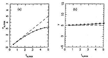
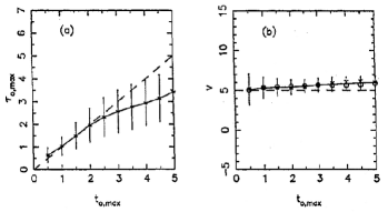
Figure 4.: Two left panels: The calculated optical depth $\tau_{\rm 0,max}$ and velocity $v$ with BCM (constant source function) versus the assumed optical thickness. The dashed curve is the model, the solid curve the inversion. Two right panels: Same plots but with added Gaussian noise. From Mein et al. (1996a).

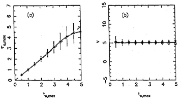
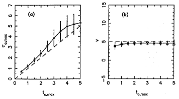
Figure 5.: Two left panels: The calculated optical depth $\tau_{\rm 0,max}$ and velocity $v$ using a cloud model with variable source function (see Eq. 5) depending only on line-center optical thickness versus the assumed optical thickness. Gaussian noise has also been taken into account. Two right panels: Same plots but for an over-estimated chromospheric background profile. From Mein et al. (1996a).

Mein et al. (1996a) presented a rather detailed study about the validity of BCM (constant source function), as well as of cloud models with a variable source function as described in Eq. 5 (depending only on line-center optical thickness) by inverting theoretical profiles produced with a NLTE code and comparing the resulting model parameters from the inversion with the assumed ones. Figure 4 (two left panels) shows the results of the inversion versus the assumed model optical thickness for the BCM inversion (constant source function). The calculated optical thickness is smaller, with the difference increasing with the thickness of the cloud, while the difference in velocity is no more than 20% and only for high values of the thickness. The figure shows that for optically thin structures there is practically no difference in the obtained results. When noise is included (Fig. 4, two right panels) the error increases for increasing thickness but the mean values stay almost the same. Again for optically thin structures the difference in the results is very small.

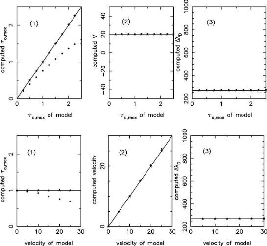
Figure 6.: Comparison of the results obtained with method (a) represented by dots and with method (b) represented by asterisks (see text for details of the methods) with the assumed model values (solid curve). From Heinzel et al. (1999).

Figure 5 (two left panels) shows the results of the inversion versus the assumed model optical thickness for a cloud model with variable source function according to Eq. 5 depending only on line-center optical thickness with an added Gaussian noise; without noise the results are perfectly reproduced. We see that the differences are now almost negligible for a large range of the assumed optical thickness and the parameters are better determined. However, when taking a slightly brighter background (Fig. 5, two right panels) we see that the calculated values of the optical thickness are larger than the assumed ones, while the estimation of velocity is still rather good. This shows the importance of a correct background profile choice in cloud model calculations.

Heinzel et al. (1999) has repeated the same exercise (inversion of NLTE synthetic profiles) for a cloud model with a variable source function according to Eq. 5 depending a) only on line-center optical thickness (method a) and b) on line-center optical thickness and velocity (method b). Some of their results are shown in Fig. 6. We see that although with method (a) there are some differences in the calculation of optical thickness, similarly to Mein et al. (1996a), method (b) gives exact solutions. Heinzel et al. (1999) have also applied the two methods in observed profiles of a dark arch filament. Figure 7 shows the comparison of the results obtained with the two methods.

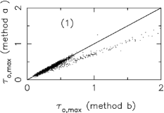
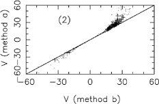
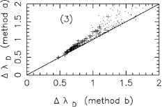
Figure 7.: Comparison of the results obtained with the two methods (a) and (b) (see text for details) from the inversion of observed profiles of a dark arch filament. Scatter plots are shown for (1) optical thickness, (2) velocity (in km s^-1), and (3) Doppler width (in Å). From Heinzel et al. (1999).

We refer also the reader selectively to a) Molowny-Horas et al. (2001) (Fig. 12 of their paper) for a comparison of inversion results for a filament with a NLTE method and a cloud model with a parabolic $S$, b) Schmieder et al. (2003) (Fig. 16 of their paper) for a comparison of inversion results for a filament with a NLTE method and a constant source function cloud model, c) Tsiropoula et al. (1999) (Fig. 5 of their paper) for a comparison of inversion results for mottles for cloud models with a constant and parabolic $S$, and d) Alissandrakis et al. (1990) (Fig. 8 to 11 of their paper) for a comparison of inversion results for an arch filament system with Beckers’ cloud model, the Doppler signal method and the differential cloud model.

5 Examples of Cloud Model Inversions

Cloud models have been so far successfully applied for the derivation of the parameters of several cloud-like solar structures of the quiet Sun, such as mottles/spicules, as well of active region structures, such as arch filament systems (AFS), filaments, fibrils, flaring regions, surges etc. Below, some examples of such cloud model inversions are presented.

5.1 Application to filaments

Filaments are commonly observed features that appear on the solar disc as dark long structures, lying along longitudinal magnetic field inversion lines. When observed on the limb they are bright and are called prominences. Filaments were some of the first solar structures to be studied with cloud models (see for example Maltby 1976, and references therein). Since then several authors used different cloud models to infer the dynamics and physical parameters of filaments. Mein, Mein & Wiik (1994), for example, studied the dynamical fine structure (threads) of a quiescent filament assuming a number of identical – except for the velocity – threads seen over the chromosphere and using a variant of BCM, while Schmieder et al. (1991) performed a similar study for threads by using the DCM. Morimoto & Kurokawa (2003) developed an interesting method applying BCM to determine the three-dimensional velocity fields of disappearing filaments.

Molowny-Horas et al. (2001) and Tziotziou et al. (2001) studied the same filament observed in H$\alpha$ and Ca II 8542 Å  respectively with the Multichannel Subtractive Double Pass (MSDP) spectrograph (Mein 1991, 2002) mounted on the German solar telescope VTT in Tenerife. The filament was studied by using two very large grids of models in H$\alpha$ and Ca II 8542 Å  respectively which were constructed with the NLTE one-dimensional code MALI (Heinzel 1995), as described in Sect. 2.6 Two-dimensional distributions of the physical parameters were obtained (see Fig. 8) which are not that similar due to the different physical formation properties and formation heights of the two lines. Schmieder et al. (2003) performed a similar NLTE grid inversion of a filament combined with a classical BCM inversion in a multi-wavelength study of filament channels. More recently, Chae et al. (2006) used H$\alpha$ images obtained with a tunable filter and a BCM inversion to obtain detailed two-dimensional distributions of the physical parameters describing a quiescent filament.

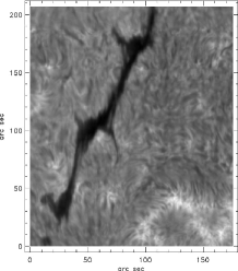
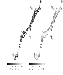
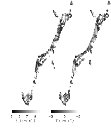
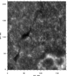
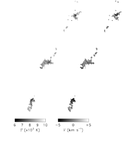
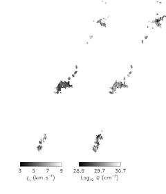
Figure 8.: Top row: A filament observed in H$\alpha$ and the two-dimensional parameter distributions derived with a H$\alpha$ NLTE inversion using a grid of models. From Molowny-Horas et al. (2001). Bottom row: Same filament observed in Ca II 8542 Å  and the two-dimensional parameter distributions derived with a Ca II 8542 Å  NLTE grid model inversion. From Tziotziou et al. (2001).

5.2 Application to arch filaments (AFS)

Arch filaments systems (AFSs) are low-lying dark loop-like structures formed during the emergence of solar magnetic flux in active regions. Georgakilas et al. (1990) have used the Doppler signal method described in Sect. 2.4 to study mass motions in AFSs observed in H$\alpha$, while Alissandrakis et al. (1990) and Tsiropoula et al. (1992) used the standard BCM to obtain the physical parameters describing arch filament regions observed in the same line (see Fig. 9). An example of the use of the differential cloud model described in Sect. 2.2 for the study of the dynamics of AFSs can be found in Mein et al. (1996b) who applied the method to H$\alpha$ observations from a two-telescope coordinated campaign. Finally Mein et al. (2000) present a study of AFSs in Ca II 8542 Å  using a fitting done with NLTE synthetic profile calculations – as described in Sect. 2.6 – with the one-dimensional MALI code (Heinzel 1995).

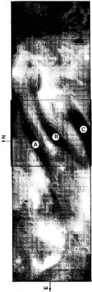
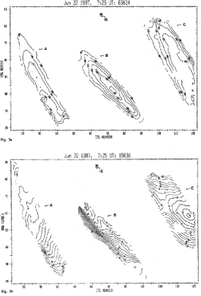
Figure 9.: Contours maps of source function (top right panel) and the velocity (bottom right panel) derived with the cloud model for the AFS shown in H$\alpha$ in the left panel of the figure. From Alissandrakis et al. (1990).

5.3 Application to fibrils

Fibrils are small dark structures, belonging to the family of “chromospheric fine structures”, found in active regions surrounding plages or sunspots (penumbral fibrils). One of the first studies of fibrils was conducted by Bray (1974) who compared observed profiles of fibrils with profiles calculated with BCM. Alissandrakis et al. (1990) used the standard BCM to obtain two-dimensional maps of several physical parameters distributions describing fibrils using H$\alpha$ observations obtained at Pic du Midi Observatory. Georgakilas et al. (2003) used filtergrams obtained at nine wavelengths along the H$\alpha$ to study the Evershed flow in sunspots and reconstruct the three-dimensional velocity vector using the Doppler signal method (see Fig. 10), while Tsiropoula (2000) used also the Doppler signal method to determine LOS velocities of dark penumbral fibrils.

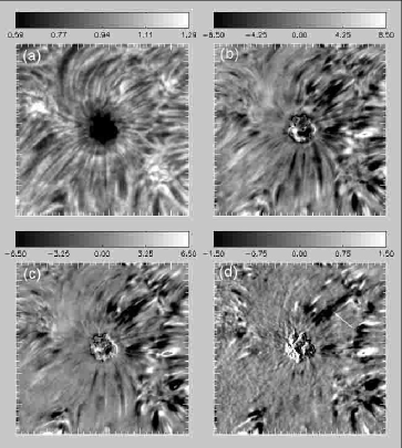
Figure 10.: Image of a sunspot observed in H$\alpha$ (a) and Doppler velocity maps computed with the Doppler signal method from filtergrams in H$\alpha$$\pm$0.35Å (b), in H$\alpha$$\pm$0.5Å (c) and in H$\alpha$$\pm$0.75Å (d). The intensity gray scale bar corresponds to normalized intensities while the Doppler velocity gray scale bars to velocities in km s^-1. From Georgakilas et al. (2003).

5.4 Application to mottles

Mottles are small-scale structures (appearing both bright and dark) belonging also to the family of “chromospheric fine structures” and occurring at quiet Sun regions at the boundaries of supergranular cells. Mottles are believed to be the counterparts of limb spicules. They form groups called chains (when they are almost parallel to each other) or rosettes (when they are more or less circularly aligned, pointing radially outwards from a central core) depending on their location at the chromospheric network.

First cloud studies of mottles started with a controversy about the ability of BCM to explain their contrast profiles. Bray (1973) and Loughhead (1973) who studied bright and dark mottles found that their contrast profiles are in good agreement with BCM. However, Loughhead (1973) used also BCM to deduce that it could not explain the contrast of individual bright and dark mottles observed in H$\alpha$ near the limb, while Cram (1975) claimed that the parameters inferred from an application of BCM to contrast profiles of chromospheric fine structures are unreliable.

Since then cloud models have been established as a reliable method for the study of physical parameters of mottles. Tsiropoula et al. (1999) studied several bright and dark mottles to derive physical parameters assuming a constant as well as a varying source function according to Eq. 6. Tsiropoula & Schmieder (1997) applied Beckers’ cloud model to determine physical parameters in H$\alpha$ dark mottles of a rosette region, while Tsiropoula et al. (1993, 1994) studied the time evolution and fine structure of a rosette with BCM and first showed an alternating behaviour with time for velocity along mottles (see Fig. 11, left panel). A similar behaviour has also been found by Tziotziou et al. (2003) using BCM for a chain of mottles (see Fig. 11, right panel), while the dynamics of an enhanced network region were also explored in high resolution H$\alpha$ images by Al et al. (2004).

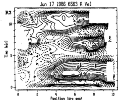
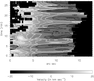
Figure 11.: Left panel: Cloud velocity as a function of position and time along the axis of a dark mottle belonging to a rosette. From Tsiropoula et al. (1994). Right panel: Cloud velocity as a function of position and time along the axis of a dark mottle belonging to a chain of mottles. White contours denote downward velocities, black upward velocities, while the thick gray curve is the zero velocity contour. From Tziotziou et al. (2003).

5.5 Application to post-flare loops

Post-flare loops are loops generally observed between two-ribbon flares. We refer the reader to Bray & Loughhead (1983) for one of the first post-flare loop studies, who constructed theoretical curves based on the cloud model to fit observed contrast profiles of active region loops. Later Schmieder et al. (1988) and Heinzel et al. (1992) used a differential cloud model to study the structure and dynamics of post-flare loops. Heinzel et al. (1992) also constructed several isobaric and isothermal NLTE models of post-flare loops. Their results were compared by Gu et al. (1997) with two-dimensional maps of H$\alpha$ post-flare loop cloud parameters obtained using a two-cloud model. Multi-cloud models like the ones described in Sect. 2.3 were used by Liang et al. (2004) to study H$\alpha$ post-flare loops at the limb (see Fig. 12), by Gu & Ding (2002) for the study of H$\alpha$ and Ca II 8542 Å  post-flare loops and by Dun et al. (2000) for the study of H$\beta$ post-flare loops. Liu & Ding (2001) obtained parameters of H$\alpha$ post-flare loops using the modified cloud model method presented in Sect. 2.5 that eliminates the use of the background profile while Gu et al. (1992) presented an extensive study using BCM, the differential cloud model and a two-cloud model to study the time evolution of post-flare loops in two-ribbon flares. Finally, we refer the reader to Berlicki et al. (2005) who studied H$\alpha$ ribbons during the gradual phase of a flare by comparing observed H$\alpha$ profiles with a grid of synthetic H$\alpha$ profiles calculated with the NLTE code MALI (Heinzel 1995) which was modified to account for flare conditions.

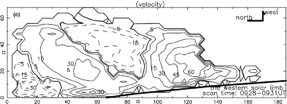
Figure 12.: The distributions of Doppler velocity (in km s^-1) derived with a multi-cloud method for H$\alpha$ limb post-flare loops. Coordinates are in units of arcsec, dashed curves show red-shifted mass motions, while solid curves indicate blue-shifted ones. From Liang et al. (2004).

5.6 Application to surges

Surges are large jet-like structures observed in opposite polarity flux emergence areas in active regions believed to be supported by magnetic reconnection. Gu et al. (1994) studied a surge on the limb observed in H$\alpha$, using a two-cloud model inversion as described in Sect. 2.3 (see Fig 13). The inversion result was detailed two-dimensional maps of the blue-shifted and red-shifted LOS velocity distributions.

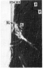
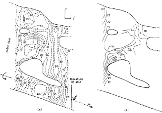
Figure 13.: An H$\alpha$ filtergram of a surge (left panle) and the two-dimensional isocontours of Doppler velocity derived with a two-cloud model. Dashed curves refer to blue-shifted velocities (middle panel), solid curves red-shifted ones (right panel), while the unit of velocity is in km s^-1. From Gu et al. (1994).

6 Conclusions

Several inversion techniques for chromospheric structures based on the cloud model have been reviewed. Cloud models are fast, quite reliable tools for inferring the physical parameters describing cloud-like chromospheric structures located above the solar photosphere and being illuminated by a background radiation. Cloud model techniques usually provide unique solutions and the results do not differ – in principle – qualitatively, especially for velocity, when using different cloud model techniques. However there can be quantitative differences arising from a) the selection of the background intensity, b) the physical conditions and especially the behaviour of the source function within the structure under study, and c) the particular model assumptions. Cloud models are mainly used for absorbing structures, however most of the techniques do work also for line-center contrasts that are slightly higher than zero, indicating an important emission by the structure itself.

Several different variants for cloud modeling have been proposed in literature so far that mainly deal with different assumptions or calculations for the source functions and span from the simple BCM that assumes a constant source function to more complicated NLTE calculations of the radiation transfer and hence the source function within the structure. Accordingly, several different techniques – most of them iterative – have been proposed for solving cloud model equations. The latest and more accurate inversion techniques involve the construction of large grids of synthetic profiles, for different geometries and physical conditions, which are used for comparison with observed profiles.

Cloud models can be applied with success to several, different in geometry and physical conditions, solar structures both of the quiet Sun, as well as of active regions. The resulting parameter inversions has shed light to several problems involving the physics and dynamics of chromospheric structures.

The future of cloud modeling looks even more brighter. New high resolution data from telescopes combined with an always increasing computer power and the continuous development of new, state of the art, NLTE one-dimensional and two-dimensional cloud model codes will provide further detailed insights to the physics and dynamics that govern chromospheric structures.

Acknowledgments.

KT thanks G. Tsiropoula for constructive comments on the manuscript and acknowledges support by the organizers of the meeting and by Marie Curie European Reintegration Grant MERG-CT-2004-021626.

References

- Al et al. (2004) Al N., Bendlin C., Hirzberger J., Kneer F., Trujillo Bueno J., 2004, A&A 418, 1131
- Alissandrakis et al. (1990) Alissandrakis C. E., Tsiropoula G., Mein P., 1990, A&A 230, 200
- Auer & Paletou (1994) Auer L. H., Paletou F., 1994, A&A 284, 675
- Beckers (1964) Beckers J. M., 1964, A study of the fine structures in the solar chromosphere, Ph.D. Thesis, Utrecht
- Berlicki et al. (2005) Berlicki A., Heinzel P., Schmieder B., Mein P., Mein N., 2005, A&A 430, 679
- Bray (1973) Bray R. J., 1973, Solar Phys. 29, 317
- Bray (1974) Bray R. J., 1974, Solar Phys. 38, 377
- Bray & Loughhead (1983) Bray R. J., Loughhead R. E., 1983, Solar Phys. 85, 131
- Chae et al. (1998) Chae, J., Yun, H.S., Poland, A.I., 1998, ApJS 114, 151
- Chae et al. (2006) Chae, J., Park, Y.-D., Park, H.-M., 2006, Solar Phys. 234, 115
- Cram (1975) Cram L. E., 1975, Solar Phys. 42, 53
- Dun et al. (2000) Dun J.P., Gu X.M., Zhong S.H., 2000, Ap&SS 274, 473
- Fontenla & Rovira (1985) Fontenla J. M., Rovira M., 1985, Solar Phys. 96, 53
- Georgakilas et al. (1990) Georgakilas A. A., Alissandrakis C. E., Zachariadis Th. G., 1990, Solar Phys. 129, 277
- Georgakilas et al. (2003) Georgakilas A. A., Christopoulou E. B., Skodras A., Koutchmy S., 2003, A&A 403, 1123
- Gouttebroze (2004) Gouttebroze P., 2004, A&A 413, 733
- Gouttebroze (2005) Gouttebroze P., 2005, A&A 434, 1165
- Gouttebroze et al. (1993) Gouttebroze P., Heinzel P., Vial J.-C., 1993, A&AS 99, 513
- Grossmann-Doerth & von Uexküll (1971) Grossmann-Doerth U., Uexküll M., 1971, Solar Phys. 20, 31
- Gu & Ding (2002) Gu X. M., Ding M. D., 2002, Chin. J. Astron. Astrophys. 2, 92
- Gu et al. (1992) Gu X. M., Lin J., Luan T., Schmieder B., 1992, A&A 259, 649
- Gu et al. (1994) Gu X. M., Lin J., Li K. J., Xuan J. Y., Luan T., Li Z. K., 1994, A&A 282, 240
- Gu et al. (1996) Gu X. M., Lin J., Li K. J., Dun J. P., 1996, Ap&SS 240, 263
- Gu et al. (1997) Gu X. M., Ding Y. J., Luo Z., Schmieder B., 1997, A&A 324, 289
- Heasley & Mihalas (1976) Heasley J. N., Mihalas D., 1976, ApJ 205, 273
- Heasley & Milkey (1976) Heasley J. N., Milkey R. W., 1976, ApJ 210, 827
- Heasley et al. (1974) Heasley J. N., Mihalas D., Poland A., 1974, ApJ 192, 181
- Heinzel (1995) Heinzel P., 1995, A&A 299, 563
- Heinzel & Anzer (2001) Heinzel P., Anzer U., 2001, A&A 375, 1082
- Heinzel & Schmieder (1994) Heinzel P., Schmieder B., 1994, A&A 282, 939
- Heinzel et al. (1987) Heinzel P., Gouttebroze P., Vial J.-C., 1987, A&A 183, 351
- Heinzel et al. (1999) Heinzel P., Mein N., Mein P., 1999, A&A 346, 322
- Heinzel et al. (1992) Heinzel P., Schmieder B., Mein P., 1992, Solar Phys. 139, 81
- Liang et al. (2004) Liang H., Zhan L., Xiang F., Zhao H., 2004, New Astron. 10, 121
- Li & Ding (1992) Li K. J., Ding Y. J., 1992, Acta Astron. Sin. 33, 171
- Li et al. (1993) Li K. J., Ding Y. J., Gu X. M., Li Q. S., Zhong S. H., Li Q. Y., 1993, A&A 269, 496
- Li et al. (1994) Li K. J., Ding Y. J., Bai J. M., Zhong S. H., Xuan J. Y., Li Q. Y., 1994, Solar Phys. 150, 87
- Liu & Ding (2001) Liu Y., Ding M. D., 2001, Solar Phys. 200, 127
- Loughhead (1973) Loughhead R. E., 1973, Solar Phys. 29, 327
- Maltby (1976) Maltby P., 1976, Solar Phys. 46, 149
- Mein (1991) Mein P., 1991, A&A 248, 669
- Mein (2000) Mein P., 2000, in J.-P. Zahn, M. Stavinschi (eds.), NATO ASIC Proc. 558: Advances in Solar Research at Eclipses from Ground and from Space, 221
- Mein (2002) Mein P., 2002, A&A 381, 271
- Mein & Mein (1988) Mein P., Mein N., 1988, A&A 203, 162
- Mein, Mein & Wiik (1994) Mein N., Mein P., Wiik, J. E., 1994, Solar Phys. 151, 75
- Mein et al. (1996a) Mein N., Mein P., Heinzel, P., Vial, J.-C., Malherbe, J. M., Staiger, J., 1996a, A&A 309, 275
- Mein et al. (1996b) Mein P., Démoulin P., Mein N., Engvold O., Molowny-Horas R., Heinzel, P., Gontikakis, C., 1996b, A&A 305, 343
- Mein et al. (2000) Mein P., Briand C., Heinzel, P., Mein, N., 2000, A&A 355, 1146
- Mihalas et al. (1978) Mihalas D., Auer L. H., Mihalas B. R., 1978, ApJ 220, 1001