Distortion of Gravitational-Wave Packets Due to their Self-Gravity

Abstract

When a source emits a gravity-wave (GW) pulse over a short period of time, the leading edge of the GW signal is redshifted more than the inner boundary of the pulse. The GW pulse is distorted by the gravitational effect of the self-energy residing in between these shells. We illustrate this distortion for GW pulses from the final plunge of BH binaries, leading to the evolution of the GW profile as a function of the radial distance from the source. The distortion depends on the total GW energy released $\epsilon$ and the duration of the emission $\tau$, scaled by the total binary mass $M$. The effect should be relevant in finite box simulations where the waveforms are extracted within a radius of $\lesssim 10^{2}M$. For characteristic emission parameters at the final plunge between binary BHs of arbitrary spins, this effect could distort the simulated GW templates for LIGO and LISA by a fraction of $10^{-3}$. Accounting for the wave distortion would significantly decrease the waveform extraction errors in numerical simulations.

I Introduction

The observation of gravitational waves (GWs) is expected to open a new window on the universe within the following decade. First generation GW detectors (InLIGO , VIRGO , TAMA , GEO ) are already operating at or close to their design sensitivity levels and the development of the next advanced-sensitivity GW detectors (Advanced LIGO , Advanced Virgo , LCGT ) and the space-detector LISA are well underway. It is now increasingly important to fully understand the precise characteristics of the GW waveforms that we expect to observe.

The most luminous GW sources are expected to be associated with mergers of BH binaries. The physical understanding of these sources has greatly improved by recent breakthroughs in numerical relativity Pretorius (2005); Campanelli et al. (2006a); Baker et al. (2006a). It is now finally possible to simulate the merger of a BH binary, from the initial circular inspiral, through the plunge to a common surrounding horizon, to the final ringdown, as the remnant settles down to a quiescent stationary Kerr-BH. It is widely believed now that existing simulations are sufficiently precise to allow targeted searches for these waveforms in real data Baker et al. (2006b). In fact, it has been recently shown that the errors are not even limited by the numerical precision of the simulation ($\sim 10^{-5}$), but the GW extraction method itself entails a much larger uncertainty ($\sim 10^{-3}$) Pazos et al. (2007). In this paper, we demonstrate that the self-gravity during the propagation of gravitational radiation in the zone of wave extraction of numerical simuations leads to the distortion of the waves, corresponding to similar magnitude modifications in typical cases.

I.1 Description of the effect

Let us imagine a compact spherically-symmetric configuration of matter (representing the remnant) and a rapidly expanding sphere of massless particles (representing the radiation) carrying away some of the initial mass of the system (Fig. 1). First, let us assume Newtonian gravity and spherical symmetry. In this case, the various shells are pulled back only by the gravity of the mass interior as if it was concentrated to a point mass at the center of the sphere, and the effect of the outer enclosing shells exactly cancels out. Thus, the particles on the outermost shell are always attracted by the total mass, including the mass of the radiation, but the innermost shells experience only the gravity of the remnant. Therefore, the gravity of the radiation implies that the innermost shells of radiation will be continuously catching up to the outer boundary during their journey from the source to the observer.

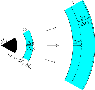
Figure 1: A sketch of the effect under consideration. The coalescence of two BHs in a binary of total initial mass $M_{0}$ results in the emission of a burst of gravitational radiation which carries away a non-negligible $\epsilon$ fraction of $M_{0}$. The remnant BH mass is $M_{f}$. The proper temporal width of the wave-packet for a hypothetical observer fixed at a radial distance $r$ is $\Delta\tau$. As the packet propagates outwards, it (1) expands due to gravitational redshift of the initial mass $M_{0}$ (solid lines), (2) contracts due to the mean self-gravity of the radiation (dotted line, $\Delta\tau^{\prime}$), and also (3) distorts its profile due to the self-gravity of the radiation (not shown). As a result the inner shells begin to catch up, and the proper time separation in excess of gravitational redshift from the front of the burst decreases with distance. Consequently, the net luminosity of the radiation burst changes with distance.

Do we expect an analogous effect to exist also for gravitational waves in full general relativity? First, let us consider conventional (i.e. non-gravitational) radiation. In analogy to the Newtonian gravitational pull, relativistic test particles are slowed down by gravity: the null-geodesics in a gravitational field experience the so-called Shapiro delay Shapiro (1964), decreasing the radial coordinate velocity with increasing gravity. Furthermore, according to Birkhoff’s theorem, the spacetime outside a spherically symmetric distribution of energy is equivalent to the spacetime of a point-mass placed at the center of the sphere, the Schwarzschild metric, and the spacetime inside a cavity is the free-space Minkowski spacetime. More generally, the spherically symmetric expansion of collisionless radiation is a known simple exact solution of the Einstein equations, the Vaidya metric Vaidya (1951); Vaidya and Shah (1960). This solution has exactly the same characteristics as the Newtonian example, whereby various shells react only to the mass interior to them, i.e. they move on world lines neglecting the exterior shells and the effect of the interior shells is the same as if they were concentrated to a point mass at the center.

Next, let us turn to the case of gravitational radiation. The effect of the self-energy of gravitational radiation can be accounted for in the first nonlinear-order approximation of the Einstein field equations by attaching terms of order $h^{2}$ to the stress-energy, $T_{ij}$, considering these terms as sources in addition to the regular radiation fields Brill and Hartle (1964); Isaacson (1968a, b); Misner et al. (1973); Thorne and Kovacs (1975); Thorne (1980); Efroimsky (1994). Here $h_{ij}$ is the wave amplitude which is the correction to the background metric. If the wavelength of the GW wave-packet is much smaller than the size of the wave envelope, the evolution of the wave-packet is determined by the WKB cycle-averaged effective stress-energy tensor Isaacson (1968a, b), independent of the specific wave-characteristics of the radiation. In this regime, we may treat the GW packet as an ensemble of relativistic particles for which our previous arguments apply. In conclusion, we anticipate that

1. the wave-envelope will continuously expand due to the redshift of the initial mass of the binary,

2. it will contract due to the self-gravity of the radiation, and

3. in analogy to electrodynamics, we expect that the distortion of the wave envelope would lead to a continuous adiabatic modification in the GW frequency.

The purpose of this paper, is to quantify these expectations for typical BH merger waveforms using simple models and to demonstrate that this effect should be accounted for in relation to numerical simulations and observed merger waveforms.

I.2 Related literature

To our knowledge the effect of self-gravitational distortion of GWs had not been explicitly recognized previously. We elaborate on the relation of the self-distortion effect to numerical general relativity, analytical investigations like the multipolar post-Minkowskian (MPM) and post-Newtonian (PN) theory, and the studies of the scattering of gravitational radiation in curved spacetimes.

The self-gravitational distortion of GWs is a relatively small effect on short scales currently accessible to numerical simulations. Current state-of-the-art simulations of binary BH mergers are restricted to the central strong-gravity domain near the black holes, and extract gravity waves from the boundary of this domain. The standard method of extracting and extrapolating the waveforms to larger distances, is based on the Regge–Wheeler–Zerilli-Moncrief perturbation formalism Regge and Wheeler (1957); Zerilli (1970); Moncrief (1974). This is a linear-order representation of the Einstein field equations and so it neglects self-energy effects of order $h^{2}$. Cumulative nonlinear effects like the self-distortion effect should lead to systematical deformations of the linear waveform extracted at different radii, which can in principle be discovered by a rigorous convergence test. In fact, nearly all papers on simulated merger GWs study the convergence behaviour in some detail. However, due to computational limitations, the extraction radius is currently restricted to $r\mathrel{\hbox to0.0pt{\lower 4.0pt\hbox{\hskip 1.0pt$\sim$}\hss}\raise 1.0pt\hbox{$<$}}50M$, and the extraction has been preformed on only a few, typically 3–4 different radii with the extrapolation done empirically based on these radii Pretorius (2005); Campanelli et al. (2006a); Baker et al. (2006a, b); Brügmann et al. (2006); Baker et al. (2004); Campanelli et al. (2006b, c); Tichy and Marronetti (2007); Pretorius and Khurana (2007); Berti et al. (2007); Buonanno et al. (2007); Baker et al. (2006c). Recently, Pazos et al. Pazos et al. (2007) reported a systematic effect of order $10^{-3}$ (for extraction radii $r\leq 80M$), which is much larger than the numerical precision of the simulation $\sim 10^{-5}$. This is roughly the same order of magnitude systematic effect that we expect for the GW distortion for the given radii (see below). Note however, that Berti et al. Berti et al. (2007) showed that the convergence behavior is also largely sensitive to simulation assumptions. On small scales probed by these simulations, other near-field nonlinearities might also be of equal importance.

A precise treatment of the waveforms at large radii is possible by analytical methods, such as the MPM-expansion introduced by Thorne Thorne (1980) (see also Thorne and Kovacs (1975)) and developed further by Blanchet & Damour Blanchet and Damour (1984, 1986, 1992). In Ref. Thorne (1980), Thorne introduced the concept of “local-wave zone,” which is outside the dynamical zone of wave generation, but where nonlinear effects are still important. In this region the propagation of gravity waves is expressed in terms of an expansion in powers of $h_{ij}$ as an infinite sum of multipole contributions with rapidly decreasing amplitude, which needs to be matched to the dynamical gravitational field generated by the source. The GWs in the local wave zone are given formally by the MPM expansion, whose terms correspond to different powers of the gravitational coupling constant $G$. In the PN approach, the dynamical wave generation is calculated analytically in an infinite series in the inverse speed of light $c^{-2}$. Matching the PN and MPM expansions in the local wave zone is a successful method for the calculation for steady source GWs produced by relatively slow motions, like the inspiral phase of BH mergers where the distance between the BHs is large enough to allow an adiabatic quasicircular orbit at $r>6M$. To date, the PN waveforms for circular binary inspirals are available to 3.5PN order for general mass ratios Blanchet (2006) (which is the highest order that is expected to have a measurable contribution for circular inspirals by a LISA-type detector Arun (2006)) and 5.5PN order for extreme mass ratios and no BH spins Tanaka et al. (1996). To our best knownledge, the self-gravitational distortion effect has not been identified in these works. However, in this paper we show that the radius for a fixed luminosity shift or a fixed frequency shift is linearly sensitive to the energy density of the radiation. The luminosity at the inspiral phase of binaries is less than $1\%$ of the luminosity at the final plunge Buonanno et al. (2007). Therefore, even if it is negligible for inspirals, the self-gravitational modulation of GWs could be significant for the final plunge.

We expect the self-gravitational distortion of GWs to be consistent with the PN/MPM expansion, and to have corresponding PN tail counterparts Blanchet (1998a). The tails of GWs are caused by the scattering of linear waves on the spacetime curvature generated by the total mass-energy of the source Wiseman and Will (1991), which is related to the Shapiro time-delay Shapiro (1964) of the radiation crawling out of the background gravity of the source. At $2.5$PN order beyond the Newtonian quadrupole formula, GW tails scatter off the monopole field of the remnant Poisson (1993); Wiseman (1993); Blanchet and Schäfer (1993). Furthermore, above 3PN order, the tails of the tails are produced by curvature scattering of the tails of the waves themselves, associated with the cubic nonlinear interaction between two mass monopole moments and the mass quadrupole of the source Blanchet (1998b). In this paper we show that the modification caused by the spherical self-gravitational distortion of GWs is to lowest order proportional to the original waveform (i.e. without this effect) times the energy density of the waveform. Since the energy density is proportional to the square of the amplitude, this possibly implies to lowest order a monopole-quadrupole² type interaction counterpart.

The self-gravitational distortion effect is also related to the “memory effects” (or “hereditary effects”) of gravitational radiation, since it is a cumulative effect that depends on the full past history of the radiation, as opposed to regular PN terms which only depend on the instantaneous retarded fields. Other known hereditary GW effects are the tails of GWs Blanchet and Damour (1992); Blanchet (1998c), the Christodoulou effect Christodoulou (1991); Thorne (1992), and the GW recoil kick Gleiser and Domínguez (2003).

Finally, nonlinear effects were also examined for the interaction of plane GWs on a free space (i.e. Minkowski) background Bonnor (1969); Aichelburg and Sexl (1971); Hayashi and Samura (1994); Mendonça and Cardoso (2002); Servin et al. (2003); Mendonça et al. (2003). The nonlinear terms in the scattering problem are found to exactly cancel up to fourth order, leaving no self-phase-modulation effect for GWs in vacuum to this order. However, the geometry of this case is very different from the one discussed in this paper where a curved background is initially present. It is also unclear whether there are self-phase modulation effects at higher nonlinear orders. Fortunately, our approach does not face such convergence issues, since we adopt the exact (i.e. non-perturbative) solution of the Einstein equations in the spherical WKB approximation of an expanding radiation shell.

The present paper aims to quantify the self-gravitational distortion effect for recently compiled merger waveforms. In § II, we list the main properties of the waveforms relevant for our study. In § III we present our analysis in spherical symmetry, and derive the results for the self-gravitational distortion of signal duration and the luminosity profile. In § IV we summarize the main conclusions, and then discuss their implications. Finally, we discuss the validity of the spherical approximation and consider the possible effect of the anisotropy in the Appendix. We use units with ${\rm G}={\rm c}=1$ and a metric signature of $(-1,1,1,1)$.

II Merger waveforms

To illustrate our effect, we adopt a simplified treatment for the merger GW waveforms. Table 1 lists the total radiated mass $\Delta m_{\rm tot}$ relative to the initial total mass $M_{0}$ for various encounters between compact objects found in the literature. While all of these encounters would have a nonnegligible GW self-gravitational effect, the inspiral–merger–ringdown events are expected to have the most prominent event rates for interferometric GW detectors. Inspiral detection rate estimates are between $0.3-3\,\mathrm{yr}^{-1}$ and several per day for NS/BH mergers for inLIGO and adLIGO, respectively Nakar et al. (2006); $3$ and $100\,\mathrm{yr}^{-1}$ for stellar BH/BH inspirals in globular clusters O’Leary et al. (2006) and in galactic nuclei Portegies Zwart and McMillan (2000) with adLIGO, respectively; $1$–$100\,\mathrm{yr}^{-1}$ and $30\,\mathrm{yr}^{-1}$ for supermassive (SMBH) and intermediate mass BH (IMBH) Wyithe and Loeb (2004); Portegies Zwart et al. (2006); Micic et al. (2007) and SMBH/SMBH inspirals Wyithe and Loeb (2003); Sesana et al. (2005) with LISA, respectively. The dynamic time of the encounter is proportional to the total mass; consequently we do not consider extreme mass ratio inspiral–mergers (EMRI), as the GW luminosity of these sources is much smaller. Although high velocity stellar BH encounters can be very bright in GWs, these events are expected to be rare, less than $1\,\mathrm{yr}^{-1}$ for adLIGO or LISA Kocsis et al. (2006). In this analysis, we focus on equal mass inspiral–merger–ringdown waveforms.

Table 1: Total radiated mass relative to the initial total mass, $\epsilon$, for bright GW encounters. For a detailed comparison of BH inspiral computations see Ref. Baker et al. (2007).

Objects	Encounter	Spins	orien-	Refs.	$\epsilon$
		$\left(\frac{S_{1}}{m_{1}^{2}},\frac{S_{2}}{m_{2}^{2}}\right)$	tation		$[\%]$
NS–BH	head-on	(0.0,0.0)		Löffler et al. (2006)	0.01
BH–BH	head-on	(0.0,0.0)		Campanelli et al. (2006d)	0.05
BH–BH	head-on	(0.1,0.1)		Campanelli et al. (2006d)	0.06
NS–BH	orbiting	(tidal,0)		Lee and Kluźniak (1999a, b)	0.1
BH–BH	head-on	(0.2,0.2)		Campanelli et al. (2006d)	0.12
BH–BH	head-on	(0.0,0.0)		Sperhake et al. (2005)	0.13
BH–BH	whirl	(0.0,0.0)		Pretorius and Khurana (2007)	0.5–3
BH–BH	grazing	(0.9,0.7)	$-\perp-$	Alcubierre et al. (2001)	0.9
BH–BH	grazing	(0.9,0.7)	$+\perp+$	Alcubierre et al. (2001)	1.0
BH–BH	grazing	(0.0,0.0)		Alcubierre et al. (2001)	1.2
BH–BH	inspiral	(0.2,0.2)	$+\parallel+$	Baker et al. (2004)	1.8
BH–BH	inspiral	(0.1,0.1)	$-\parallel-$	Baker et al. (2004)	2.0
BH–BH	inspiral	(0.2,0.2)	$-\parallel-$	Baker et al. (2004)	2.0
BH–BH	inspiral	(0.8,0.8)	$-\parallel-$	Campanelli et al. (2006c)	2.2
BH–BH	inspiral	(0.1,0.1)	$+\parallel+$	Baker et al. (2004)	2.4
BH–BH	inspiral	(0.0,0.0)		Baker et al. (2004)	2.5
BH–BH	inspiral	(0.0,0.0)		Baker et al. (2006a); Campanelli et al. (2006b)	3.2
BH–BH	inspiral	(0.0,0.0)		Campanelli et al. (2006c); Brügmann et al. (2006)	3.5
BH–BH	inspiral	(0.0,0.0)		Baker et al. (2006c); Berti et al. (2007)	3.7
BH–BH	inspiral	(0.1,0.1)	$+\parallel+$	Buonanno et al. (2007)	5.2
BH–BH	inspiral	(0.8,0.8)	general	Tichy and Marronetti (2007)	5–6
BH–BH	inspiral	(0.8,0.8)	$+\parallel+$	Campanelli et al. (2006c)	6.7
BH–BH	r.whirl	(0.0,0.0)		Pretorius and Khurana (2007)	15
BH–BH	r.head-on	(0.0,0.0)		D’Eath and Payne (1992)	16
BH–BH	r.head-on	(1.0,0.0)	$\perp$	Cardoso and Lemos (2003)	17$\frac{\eta}{1/4}$
BH–BH	whirl	(0.0,0.0)		Pretorius and Khurana (2007)	24
BH–BH	r.whirl	(0.0,0.0)		Pretorius and Khurana (2007)	100

Generally, the waveforms can be expanded in multipoles Thorne (1980)

$$h_{\mu\nu}=\sum_{n}\frac{(1+z){\cal A}^{n}_{\mu\nu}}{d_{L}}e^{i\phi_{n}}$$ (1)

where $\phi$ is the high frequency GW phase which is related to the instantaneous frequency through $f=\mathrm{d}\phi/\mathrm{d}t$; ${\cal A}_{\mu\nu}$ is a slowly varying envelope describing how the instantaneous amplitude changes over the waveform, the index $n$ labels the various polarizations and multipoles, and $d_{L}$ is the luminosity distance, and $z$ is the redshift. For binary inspiral merger waveforms, the ($l=2,m=2$) multipole (i.e. quadrupole) dominates the waveform Buonanno et al. (2007); Baker et al. (2006c); Berti et al. (2007). For the sake of simplicity, we restrict our attention to a single monochromatic wave.

During a single GW cycle, corresponding to a time interval $f^{-1}$, the envelope $A_{\mu\nu}$ can be regarded as constant. In the WKB approximation, the energy carried by the radiation can be calculated as a cycle-averaged quantity. The effective stress-energy tensor of the radiation is Isaacson (1968b); Misner et al. (1973)

$$T^{\mu\nu}=\frac{1}{64\pi}\frac{A^{2}}{d_{L}^{2}}k^{\mu}k^{\nu},$$ (2)

where $A^{2}={\cal A}^{\mu\nu}{\cal A}_{\mu\nu}$ is the squared effective amplitude and $k_{\mu}=\phi_{,\mu}$ is the wave number.

Each infinitesimal volume of the wave can be attributed the mass-energy that it carries according to Eq. (2). In the spherically symmetric approximation, the total luminosity (or more precisely the graviton number) is Isaacson (1968b)

$$L=\frac{\mathrm{d}E}{\mathrm{d}r\mathrm{d}t}=4\pi r^{2}T^{tr}=\frac{A^{2}}{16}k^{t}k^{r}$$ (3)

With this equation it is possible to obtain the waveform $[A(t),f(t)]$ within radius $r$ from the luminosity function $L(t)$.

Based on the waveforms derived by numerical simulations (such as Fig. 25 in Ref. Buonanno et al. (2007)), we adopt the following simple fit to the effective luminosity

$$L(t)=L_{0}\times\left\{\begin{array}[]{cc}[(t_{1}-t)/t_{1}]^{-1.5}&\text{if~{}}-t_{0}<t<0\\ 1&\text{if~{}}0<t<t_{1}\\ \exp[-(t-t_{1})/t_{2}]&\text{if~{}}t>t_{1}\\ \end{array}\right.$$ (4)

where the intervals $t<0$, $0<t<t_{1}$ and $t_{1}>t$ correspond to the late inspiral/final orbits, the peak luminosity at the plunge, and the ringdown phases, respectively, $-t_{0}$ sets the initial time of the calculated profile, $t_{1}$ represents the characteristic timescale of the most intensive part of the radiation, $t_{2}$ sets the ringdown decay rate, and $L_{0}$ is the normalization luminosity. Numerical simulations show Buonanno et al. (2007) that the characteristic frequency of the radiation rapidly increases after the inspiral and saturates at $\omega=2\pi f\sim M_{0}^{-1}/2$ at $t\sim 0$, where $M_{0}$ is the initial mass of the source. The characteristic number of wave cycles during the brightest phase is $N=\Delta t/f^{-1}\sim 3$ over a time $\Delta t=12\pi M_{0}$. Note that we assume that the WKB method is applicable to the waveform, implying that $L(t)$ does not change greatly over a single cycle. This condition is just marginally satisfied for these waveforms.

For a simple analysis, we assume that the total luminosity crossing a sphere at infinity $L_{\infty}(t)$ is given by Eq. (4) with the following parameters: $(t_{0},t_{1},t_{2})=(100,10,5)M_{0}$, and use $\Delta t=12\pi M_{0}$ in reference to average quantities below. Under the WKB approximation the luminosity (4) evolves independently of the carrier frequency $f\sim 1/(4\pi M_{0})$. The $L_{0}$ normalization is set using the total radiated mass of the system as a fraction of $M_{0}$ by $\epsilon=\Delta m_{\mathrm{tot}}/M_{0}$ for the inspiral-mergers (3) listed in Table 1. For pedagogical comparison purposes we distinguish the inspiral events only based on the normalization $L_{0}$, and do not consider the variations in the shape of the waveform (e.g. $\Delta t$).

III Quantitative estimates in spherical symmetry

To give a first quantitative estimate of the magnitude of the wave-packet distortion due to self-energy, we start by computing the propagation of unpolarized radiation packets in the spherically symmetric Vaidya spacetime. The possible effect of anisotropies is discussed in the Appendix.

The Vaidya metric Vaidya (1951) in radiation coordinates $(u,r,\theta,\phi)$ is

$$\mathrm{d}s^{2}=-\left(1-\frac{2m(u)}{r}\right)\mathrm{d}u^{2}-2\mathrm{d}r\mathrm{d}u+r^{2}\mathrm{d}\Omega,$$ (5)

where $d\Omega=d\theta^{2}+\sin^{2}\theta d\phi^{2}$. This metric is an exact (i.e. nonperturbative) solution of Einstein’s equations in spherical symmetry in the eikonal approximation to a radial flow of unpolarized radiation. Here $u$ is the retarded time parameter which is constant along the world lines of radially outgoing radiation, and $m(u)$ describes the mass function interior to $u$. Outside the radiation (i.e. where $m(u)$ is constant in the space-time), the Vaidya metric (5) is the Schwarzschild solution in Eddington-Finkelstein coordinates Misner et al. (1973). For our approximate waveforms decribed in § II, $m(u)$ is $M_{0}$ constant outside, it is quickly changing within a short range $0\leq u\leq\Delta u_{\mathrm{tot}}$ across, and it is $M_{f}=M_{0}-\Delta m_{\mathrm{tot}}$ inside the radiation shell. Here, $\Delta m_{\mathrm{tot}}$ and $\Delta u_{\mathrm{tot}}$ are set by the simulated waveforms § II.

For the metric given by Eq. (5) it is straightforward to derive the convergence of null-geodesics describing the world lines of radiation shells using Raychaudhuri’s equation or the equation of geodesic deviation Wald (1984). In either way, we find that radially outgoing shells of radiation simply follow the world lines $u(r)=\rm constant$, implying that the $\Delta u$ coordinate difference between the shells does not change during the propagation. The physical contraction of radiation shells can be examined using the proper time measure between shells and the observed luminosity profile.

III.1 Proper time duration

First, we estimate the proper-time duration of the GW signal along the world-line of a hypothetical observer crossing the radiation shell. For simplicity, we restrict to observers at a fixed spacial coordinate $(r,\theta,\phi)$. Then we have $\mathrm{d}r\equiv\mathrm{d}\theta\equiv\mathrm{d}\Omega\equiv 0$ and Eq. (5) gives

$$\mathrm{d}\tau^{2}=-\mathrm{d}s^{2}=\left(1-\frac{2m(u)}{r}\right)\mathrm{d}u^{2}$$ (6)

leading to $\mathrm{d}\tau=\sqrt{1-2m(u)/r}\mathrm{d}u$. Therefore, $\mathrm{d}u$ can be interpreted as the infinitesimal proper time difference between two radiation shells at fixed radius approaching infinity. Thus, we adopt the notation $\mathrm{d}u\equiv\mathrm{d}\tau_{\infty}$, and similarly $\Delta u\equiv\Delta\tau_{\infty}$ for integrated quantities. Finally, let us define $m_{i}=m(u_{i})$ for $i\in\{1,2\}$ and $\Delta m=|m_{2}-m_{1}|$. We set $(m_{1},m_{2},\Delta m_{\mathrm{tot}})=(M_{0},M_{f},\epsilon M_{0})$ when referring to the total GW signal duration.

Integrating between two arbitrary shells of radiation $u_{2}$ and $u_{1}$ gives

$$\Delta\tau=\int^{\tau_{2}}_{\tau_{1}}\mathrm{d}\tau=\int^{u_{2}}_{u_{1}}\left(1-\frac{2m(u)}{r}\right)^{1/2}\mathrm{d}u.$$ (7)

After expanding $m(u)$ in a Taylor-series, the integrand becomes

$$\left(1-\frac{2m_{1}}{r}-\frac{2u\langle m^{\prime}\rangle}{r}-\frac{u^{2}\langle m^{\prime\prime}\rangle}{r}+\dots\right)^{1/2}.$$ (8)

Substituting in Eq. (7), and using $\langle m^{\prime}\rangle=-\Delta m/\Delta\tau_{\infty}$ and $\langle m^{\prime\prime}\rangle=0$ to first order, we get

$$\Delta\tau(m_{1},m_{2},r)=\frac{r\Delta\tau_{\infty}}{3|m_{2}-m_{1}|}\left.\left(1-\frac{2m}{r}\right)^{3/2}\right|^{m_{2}}_{m_{1}}.$$ (9)

Setting $m_{1}=M_{0}$ and expanding in terms of $\Delta m$, we get

$$\frac{\Delta\tau}{\Delta\tau_{\infty}}=\sqrt{1-\frac{2M_{0}}{r}}\left(1+\frac{1}{2}\frac{\Delta m}{r-2M_{0}}+{\cal O}(\Delta m^{2})\right).$$ (10)

The leading order term can be indentified as the gravitational redshift for constant mass $M_{0}$, the second term describes the correction due to the radiation mass. If we expand also in terms of powers of $1/r$, the relative change in the proper time duration of the signal becomes

$$\frac{\Delta\tau-\Delta\tau_{\infty}}{\Delta\tau_{\infty}}=-\left(M_{0}-\frac{\Delta m}{2}\right)\frac{1}{r}+{\cal O}(r^{-2},\Delta m^{2}).$$ (11)

Equations (9–11) describe the self-gravitational distortion between radiation shells in terms of proper time along world lines of $r=\rm const$. One can notice that to leading order this is simply the gravitational redshift for the average enclosed mass between the shells. However, since $\Delta m$ changes along the wave packet non-trivally for a fixed radius as a function of time, the modification of the profile is generally not self-similar, leading to the distortion of the luminosity profile as a function of radius.

To make this point clearer, we correct for the average distortion of the signal and calculate the residual distortion of the signal. Let us define

$$\Delta\tau^{\prime}=(1+z)\Delta\tau-\Delta\tau_{\infty}$$ (12)

where $(1+z)$ is a time-independent constant representing the “average gravitational redshift” at a given $r$, given by

$$1+z=\frac{1}{\sqrt{1-\frac{2\langle m\rangle}{r}}},$$ (13)

$\langle m\rangle\equiv(m_{1}+m_{2})/2$ is the average mass, and to leading order

$$z\approx\frac{\langle m\rangle}{r}=\frac{M_{0}}{r}-\frac{\Delta m}{2r}.$$ (14)

Now let us take an arbitrary radiation shell enclosing mass $\Delta m$ relative to the shell enclosing mass $M_{0}-0.5\Delta m_{\mathrm{tot}}$, i.e. we set $m_{1}=M_{0}-0.5\Delta m_{\mathrm{tot}}$ and $m_{2}=m_{1}-\Delta m$ in eq. (9). After correcting for the average gravitational redshift using Eqs. (12) and (13), the residual relative distortion to leading order is

$$\frac{\Delta\tau^{\prime}}{\Delta\tau_{\infty}}=-\frac{\Delta m}{2r}+{\cal O}(r^{-2},\Delta m^{2}).$$ (15)

Figure 2: The residual self-gravitational distortion of shells after correcting for the bulk gravitational redshift. The thick curves show the change in the proper time duration of the signal at radial distance $r$ from the source between shells enclosing $7\%$ (top) or $3\%$ (bottom) of the total mass, dotted lines correspond to the leading order term given by Eq. (15). The vertical lines highlight the typical radii used in numerical simulations for GW extraction.

Figure 2 shows the residual distortion using the exact formula (Eq. (12), thick lines) and the leading order contribution (given by Eq. (15), dotted lines). At the typical radius used by numerical simulations for waveform extraction, $r=50\mathrm{M}_{\odot}$, the primary bulk waveform distortion changes the signal duration by $M_{0}/r\sim 2\%$, and the secondary relative waveform distorsion between the front and the back of the signal is $\epsilon M_{0}/(2r)\sim 7\times 10^{-4}$ for a typical BH inspiral–merger with high spins $\epsilon=7\%$ (see § II). The figure also shows that the higher order effects beyond $1/r$ lead to an uncertainty of order $10^{-3}$–$10^{-4}$ for $r=(30$–$50)M_{0}$.

III.2 Luminosity Profile

Since Eqs. (9) and (11) are applicable to two arbitrary shells of radiation, we can use them to compute the evolution of an arbitrary initial radiation profile, whereas the luminosity is simply $L=\Delta m/\Delta\tau$, the total mass-energy crossing a sphere at radius $r$ within proper time $\Delta\tau$.

The profile at infinity is given by $m(u)$ in radiation coordinates, or $\Delta\tau_{\infty}(m)$, the proper time a shell enclosing mass $m$ arrives at $r=R$ where $R\rightarrow\infty$, relative to the outermost shell of radiation . Here $\Delta\tau_{\infty}(m)$ can be any monotonically decreasing function, for which the luminosity at $R$ in Eq. (3) is

$$L_{\infty}(\tau)=-\left[\frac{\mathrm{d}\Delta\tau_{\infty}(m)}{\mathrm{d}m}\right]^{-1},$$ (16)

where the minus sign originates from our definition of $m$: the shell labeled by the largest value of $m$ arrives the earliest. The luminosity profile can also be obtained as the function of time, $L_{\infty}(\tau)$, using the relationship $\Delta\tau(m)$. Conversely, for given $L_{\infty}(\tau)$, we can compute $\Delta\tau_{\infty}(m)$ using Eq. (16). The luminosity at some other distance $r$ can be obtained similarly if given $\Delta\tau(m,r)$, the arrival time of mass $m$ relative to the outermost shell at distance $r$. This function is given by Eq. (9), substituting the waveform $\Delta\tau_{\infty}(m)$ for $\Delta\tau_{\infty}$, and $(m_{1},m_{2})=(M_{0},m)$. The luminosity profile at $r$ is then

$$L_{r}(m)= -\left[\frac{\partial\Delta\tau(m,r)}{\partial m}\right]^{-1}=\left(1-\frac{2m}{r}\right)^{-1/2}L_{\infty}(m)$$ (17)

Therefore, the modification of the profile in Bondi radiative coordinates $(m,r)$ the profile is distorted self-similarly. However, in terms of the observer proper time variable, $\Delta\tau(m)=\int_{0}^{m}L_{r}(m)^{-1}\mathrm{d}m$, $L_{r}(\tau)$, the modification to the profile will not be self-similar:

$$L_{r}(\tau)=\left(1-\frac{2\int_{0}^{\tau}L_{r}(\tau^{\prime})\mathrm{d}\tau^{\prime}}{r}\right)^{-1/2}L_{\infty}\left(\int_{0}^{\tau}L_{r}(\tau^{\prime})\mathrm{d}\tau^{\prime}\right)$$ (18)

Equation (18) relates the luminosity profile as a function of proper time at radius $r$, $L_{r}(\tau)$, to the profile at infinity, $L_{\infty}(\tau)$. Comparing Eqs. (17) and (18) shows the advantage of Bondi type radiative coordiantes as opposed to proper time.

Figure 3: Our fits to the GW luminosity profile for binary BH inspiral merger simulations as a function of observer proper time $\tau$ and the evolution of the profile at various distances, $r$. The profile parameters are given in § II and $\epsilon=7\%$. Top: The absolute profile (in units of ${\rm c}^{5}/{\rm G}$) is shown for two extremes, a nearby distance ($r=12.5M_{0}$) and far-away distance ($r=10^{3}M_{0}$). Bottom: The difference between the GW luminosity profiles at infinity (i.e. $r=10^{3}M_{0}$) and three cases of smaller $r$, in units of peak luminosity at infinity. The peaks of the profiles are set to $\tau=0$. The main effect responsible for the differences seen in this figure is the bulk gravitational redshift.

Figure 3 plots $L_{r}(\tau)$ for our fit to the luminosity profile at infinity of merging binary BHs $L_{\infty}(\tau)$ with $\epsilon=7\%$ (see § II). The top panel shows the absolute profile while the bottom panel shows the difference between the profile at some radius $r$ and the profile at infinity, such that the peak of the profiles are at $\tau=0$. The bottom panel is useful to visualize the characteristic evolution of the profile.

Figure 4: The residual self-gravitational distortion to the luminosity profiles after accounting for the avarage gravitational redshift, $z=M_{0}/r$ (top) or $(M_{0}-0.5\Delta m_{\mathrm{tot}})/r$ (bottom), respectively. Other parameters are the same as in Fig. 3.

In § III.1, we have identified the two main effects responsible for the convergence rate of the waveform to be the gravitational redshift corresponding to the average mass and the self-gravitational effect. Indeed, the differences visible in Figure 3 are primarily due to the former. However, correcting for only the average gravitational redshift at each radius $r$ leaves a nonnegligible systematic error with respect to the true signal. To see this, we substitute $\Delta\tau_{\infty}/(1+z)$ given by Eq. (13) into Eqs. (16) and (17), and refer to the corresponding luminosity as the average gravitational redshifted luminosity profile, $L_{r}^{z}(\tau)$. After subtracting from the true profile for each $\tau$, the residual luminosity distortion is

$$L^{\prime}_{r}(\tau)=L_{r}(\tau)-L_{r}^{z}(\tau),$$ (19)

where we set the reference time again to $\tau=0$ for the peak of the luminosity profiles.

Figure 4 shows the residual self-gravitational distortion $L^{\prime}_{r}(\tau)$ for various radii in units of the peak luminosity at infinity, $L_{\infty,\max}$. Naturally, the definition of the “average gravitational redshift,” $z$, used for defining $L^{\prime}_{r}(\tau)$ makes a difference in the result. The top panel uses only the initial binary mass $\langle m\rangle=M_{0}/r$ in Eq. (14) totally neglecting the gravity of the radiation shell, while the bottom panel has $\langle m\rangle=(M_{0}-0.5\Delta m_{\mathrm{tot}})/r$, i.e. the redshift is chosen to account also for the average gravity of the radiation shell. In the later case we find a much quicker convergence for the waveform peak at increasing radii, but the former choice is more suitable for the early parts of the waveform corresponding to the late inspiral waveform. A comparison of Fig. 3 and 4 shows that the self-gravitational distortion is roughly an order of magnitude smaller than the effect of the average gravitational redshift.

III.3 Self-Gravitational Coordinate Effects

In the previous sections we have derived the time duration and the luminosity profile of the radiation shell as it propagates radially outward from the source. We have assumed that the GW profile at each fixed arial radius $r$ is parameterized by the proper time $\tau$ of a hypothetical observer fixed at that radius, in particular the luminosity $L_{r}(\tau)$ was the total mass-energy crossing a sphere at radius $r$ within infinitesimal proper time $\mathrm{d}\tau$. Therefore, the adopted time-coordinate $\tau$ corresponds to a synchronous gauge at each radius. Since physical observables depend precisely on proper measures, these coordinates allow a simple interpretation of the convergence characteristics of the GW profile at large radii.

Other choices of coordinates would have introduced additional artificial distortion effects making the convergence characteristics of the waveforms much different. Consider for instance the “natural” coordinate system $(t,r,\theta,\phi)$ in the spherically symmetric case that is chosen to be Schwarzschild both before and after the GW burst has arrived with masses $M_{0}$ and $M_{f}=M_{0}-\Delta m_{\mathrm{tot}}$, respectively, and which changes smoothly in between these regions. An example of such a coordinate system can be derived from the Vaidya metric Eq. (5) with the implicit transformation $t\equiv u+r+2m(u)\ln[r-2m(u)]$ where $m(u)$ describes the mass function interior to $u$ (which is constant along the outgoing radiation world lines). Indeed, everywhere in the spacetime where $\mathrm{d}m/\mathrm{d}u=0$, these coordinates yield a Schwarzschild metric, and the Vaidya metric in radiation coordinates (5) is then simply the Schwarzschild solution in Eddington-Finkelstein coordinates Misner et al. (1973) in these regions. This map covers all relevant parts of the spacetime including the GW zone. The world-lines of radiation shells can be shown to follow

$$\frac{\mathrm{d}r}{\mathrm{d}t}=1-\frac{2m_{u}}{r},$$ (20)

where the second term is called the Shapiro-time delay Shapiro (1964) for a particle crawling out of the gravitational potential of mass $m_{u}$ interior to it. After integration, we find that to first order the temporal separation of two radiation shells enclosing mass $\Delta m$ at radius $r$ evolves to leading order as $\Delta t(r)=\Delta t(R_{0})-2\Delta m\ln(r/R_{0})$, where $R_{0}$ is an arbitrary initial radius. In these coordinates, the signal duration contracts uniformly in exponential distance intervals. Even though the metric is asymptotically Minkowski (where $t$ approaches $\tau$ for $r\gg M_{0}$), the resulting profile evolution is fundamentally different from $\Delta\tau(r)$ given by Eq. (11)!

The appearance of the logarithmic radial dependence of the waveform was first realized by Fock Fock (1959). This effect is specific to the harmonic coordinates and can be avoided if changing to Bondi type radiative coordinates Isaacson and Winicour (1968); Madore (1970). Blanchet & Schäfer Blanchet and Schäfer (1993) have shown that a similar logarithmic dependence of the GW tail leads to a tail-induced amplitude and phase shift (typically of order $10^{-7}$) for stationary sources. In contrast, the logarithmic radial dependence of the wave contraction for merger waveforms can be significant for GW merger simulations. Between $r=(20$–$40)M_{0}$, the waveform contracts in $\Delta t$ by a fraction of $5\times 10^{-3}$, which is just of the order of the current wave extraction precision Pazos et al. (2007); Baker et al. (2006c); Buonanno et al. (2007). This apparent logarithmic contraction effects can be avoided if one changes to the proper time variable as we have done in the previous sections. The remaining $\Delta\tau(r)$ evolution is however a physical effect.

Both the logarithmic $\Delta t(r)$ contraction and the physical $\Delta\tau(r)$ evolution (in particular the contribution denoted by $\Delta\tau^{\prime}(r)$ above) are consequences of higher order radiation effects in the Einstein equations beyond the scope of first order methods such as the Regge–Wheeler–Zerilli-Moncrief perturbation method used for extrapolating the numerical waveforms to infinity. Therefore these effects cause the extrapolated waveforms to be different when extracting GWs from numerical simulations at various radii by standard methods using no self-gravitational interaction. For a related recent analysis see Ref. Lehner and Moreschi (2007).

IV Discussion

IV.1 Summary

We considered the self-gravitational effect of gravitational radiation on the propagation of GWs from a compact source. We adopted simple approximations for the geometry of the radiation, by considering spherical symmetry on scales comparable to the radial width of the radiation packet. This approximation appears adequate for the quadrupolar $(l=2,m=2)$ radiation pattern around binary BH sources in numerical simulations Buonanno et al. (2007); Baker et al. (2006c); Berti et al. (2007). Nevertheless, we use the Appendix to examine the maximal effects of anisotropy in the opposite (exaggerated) extreme, when the outgoing radiation is concentrated into a compact region. We find that irrespective of the level of anisotropy, the gravitational radiation is distorted under the influence of its own gravity as it propagates. Contrary to the standard gravitational redshift, which is a uniform shift of the waveform, the self-gravitational effect depends on the intensity and is predominant only for the most intensive bursts of radiation causing a non-uniform distortion of the waveform. The self-gravitational distortion depends on distance to leading order as $\Delta m/r$, and is therefore relevant on scales $r_{\rm sg}/M_{0}\mathrel{\hbox to0.0pt{\lower 4.0pt\hbox{\hskip 1.0pt$\sim$}\hss}\raise 1.0pt\hbox{$<$}}\epsilon/\delta$ where $\epsilon$ is the radiation efficiency and $\delta$ is the desired calculation accuracy. For BH binary mergers simulations $\epsilon\sim 7\%$ and $\delta\sim 10^{-5}$ implying that $r_{\rm sg}\mathrel{\hbox to0.0pt{\lower 4.0pt\hbox{\hskip 1.0pt$\sim$}\hss}\raise 1.0pt\hbox{$<$}}7\times 10^{3}M_{0}$. If the GWs are extracted within this region, the self-gravitational distortion should be taken into account.

IV.2 Testing the Effect with Numerical Simulations

Numerical simulations based on the full set of Einstein equations for binary BH inspirals have not yet reported evidence for the waveform distortion effect considered here although they have shown that the waveforms do not converge within a fractional accuracy of $\delta\sim 10^{-3}$ Baker et al. (2006c); Buonanno et al. (2007); Pazos et al. (2007). This is because the simulations are restricted to a limited volume, typically of radii $\sim(80$–$850)M$, while the extracted waveforms are typically compared between $r\sim 20$–$50M$. For a radiation mass $\Delta m/M_{0}\sim 7\%$, the primary effect is a shift of the waveform due to a logarithmic Shapiro time delay of the remnant, a uniform gravitational redshift, and the self-gravitational effect. We have shown that the logarithmic Shapiro delay does not show up if using proper measures to describe the waveform, and the uniform gravitational redshift is accounted for in the linear wave propagation models. However, the residual self-gravitational effect in the GW luminosity has a characteristic profile that has to be subtracted when extrapolating the extracted waveform. The peak of the effective luminosity distortion reaches $2\times 10^{-3}$ and $5\times 10^{-4}$ at $r=30$ and $50M_{0}$, respectively.

Present-day numerical relativity simulations should already be capable of directly measuring the relevance of our effect by artificially amplifying the gravitational radiation found at the extraction radius $r\sim 20M$, and starting the simulation with these amplified initial conditions. For example, for a total GW energy $\Delta m/M_{0}=30\%$, the effective luminosity distortion between $r=20M$ between $20$–$50M$ is several percent, which is well within simulation and extraction errors. For consistency, the simulation should confirm that the total energy content of the radiation does not change. We also expect the initial ringdown frequency (corresponding to the most energetic shell) to be smaller than the final ringdown frequency.

In order to avoid errors caused by the self-gravitational distortion effect up to the desired numerical precision $\delta\sim 10^{-5}$, the waveform extraction radius should be chosen to be $r_{\rm sg}\mathrel{\hbox to0.0pt{\lower 4.0pt\hbox{\hskip 1.0pt$\sim$}\hss}\raise 1.0pt\hbox{$>$}}7\times 10^{3}M_{0}$. Alternatively, if the waveforms are extracted at smaller radii, the waveforms should be converted to Bondi type radiative coordinates and then extrapolated with the scaling $1/r$.

IV.3 Observational Implications

The self-gravitational waveform distortion is important for future observations of BH binary mergers.

1. The waveform distortion is expected to be resolvable for the LISA instrument with respect to simulated waveforms for total BH masses of $(10^{4}$–$10^{9})\mathrm{M}_{\odot}$. The total signal to noise ratio of merger waveforms is $10^{4}$ for LISA observing $z_{c}\sim 1$ Baker et al. (2006b). The distortion effect modifies the waveform amplitude and frequency by $\sim(10^{-3}$–$10^{-4})$ for numerical waveforms extracted between $r=(30$–$80)M_{0}$.

2. The distortion involves a systematic modification of the waveform which needs to be accounted for in order to interpret observed merger waveforms and improve the estimation uncertainty of physical parameters beyond the uncertainty of the preceding inspiral signal. The signal to noise ratio of the final BH merger waveform is an order of magnitude larger than for the inspiral, implying that the merger waveform has a potential to greatly reduce parameter estimation errors. Note that the relative accuracy using only the inspiral signal with LISA is expected to be $10^{-3}$–$10^{-5}$ Lang and Hughes (2006, 2007) for estimating the component masses, which is smaller than the distortion effect.

3. This effect is different from the uncertainties caused by gravitational lensing Holz and Hughes (2005), in that it is only an issue concerning the convergence properties of numerical simulations. Lensing causes an error of several percent on the inferred luminosity distance (due to the unresolved matter along the line of sight), and lensing errors increase with the source distance. In contrast, the self-gravitational effect is of order 0.1-0.01 percent for numerical simulations if the waveforms are extracted at $30M$–$80M$ and dies off quickly as $1/r$. The wave distortion effect is of order $10^{-20}$ relative to the waveform amplitude for typical astrophysical scales. Therefore, the wave-contraction effect does not provide any additional physical parameters for observations.

Appendix A Anisotropy

Our analysis considered only perfectly spherically-symmetric configurations. The approach was motivated by the quasi-spherical radiation patterns found around binary BH sources in numerical simulations Buonanno et al. (2007); Baker et al. (2006c); Berti et al. (2007). In this Appendix, we would like to examine the sensitivity of our basic results to deviations from sphericity. To gauge whether there is any such sensitivity, we analyse the most extreme case in which the outgoing radiation is concentrated into a highly compact region.

But first let us define more precisely what we assumed so far. The derivation presented in § III requires that the radiation field is “initially locally spherically symmetric”, so that it is initially described by the Schwarzschild metric locally within some narrow solid angle $\Delta\theta\mathrel{\hbox to0.0pt{\lower 4.0pt\hbox{\hskip 1.0pt$\sim$}\hss}\raise 1.0pt\hbox{$<$}}\Delta r/r$ before the GW arrives, where $\Delta r\sim c\Delta t$ is the radial width of the wave-packet along its propagation direction. But since the radiation propagating through this solid angle is in no causal contact with the radiation field expanding towards other directions, it cannot distinguish the actual spacetime from a spherically symmetric one. Note that the outermost shells of radiation expanding along different directions are always causally disconnected by definition, and the interior shells of radiation can only be affected by the outer shells within $\Delta\theta$. Since we examine the distortion effect on large distances compared to the width of the burst $r\gg\Delta r$, spherical symmetry must only be required within a very narrow angle. This simple set of considerations implies that if high-order multipoles have a vanishing contribution at large distances, the results derived in § III are applicable very generally for short bursts of radiation, $\Delta r\ll r$. Indeed, numerical simulations confirmed that the dominant contribution to the wave amplitude is given by the ($l=2,m=2$) multipole and higher order terms are suppressed by more than a factor of magnitude (see references in § II). In the remainder of this Appendix we demonstrate the validity of this simple conclusion through explicit calculations.

We consider three variations on a toy model to estimate the effect of anisotropy. We start with the simplest model and refine this model by adding more details and complexity in the successive models. In each case, we discuss general implications for the model under consideration. In all models we consider the extreme opposite regime to spherical symmetry, namely that the radiation is maximally clumped into two outgoing BHs $L$ (leading) and $T$ (trailing) of masses $m_{L}$ and $m_{T}$, representing the leading and trailing edges of the radiation, respectively. We assume that $L$ and $T$ are moving in the same direction on light-like world lines, so that $T$ lies in the causal past of $L$, but $L$ is outside the causal past of $T$ throughout their propagation. We assume that there is also a remnant Schwarzschild BH $R$ with mass $m_{R}$. The instantaneous radial position coordinate of $R$, $T$, and $L$ at time $t$ are $0$, $r_{T}(t)$, and $r_{L}(t)$. We are interested in obtaining the world lines of BHs $T$ and $L$ to see how the coordinate separation $\Delta r(t)=r_{L}(t)-r_{T}(t)$ decreases with time as compared to the spherically symmetric result. In our first model we neglect the remnant $R$ (setting $m_{R}=0$), assume that $L$ moves with constant velocity $v_{L}$ in free space, and calculate the trajectory of $T$ in the spacetime created by $L$. Subsequently, we will generalize $L$ to move on a more general world line with a slowly changing velocity $v_{L}(t)$. Finally, we can turn on the remnant $R$ in addition to $L$, and include the retardation effect when calculating the relative motion of $T$.

We note that the spacetime of BHs moving at the speed of light have been calculated previously in Ref. Hayashi and Samura (1994), which found that BHs moving in the same direction do not interact. However, Ref. Hayashi and Samura (1994) assumed that the BHs move in free space and consequently adopted $v=1$ for their velocity. In contrast, the BHs $T$ and $L$ travel on null-geodesics in the perturbed spacetime which is initially the Schwarzschild spacetime. This difference gives rise to a non-trivial interaction between the BHs $T$ and $L$.

We compare our results to the spherical case, using the $(t,r)$ coordinate system defined by Scwarzschild coordinates before and after the radiation shells as described in § III.3.

A.1 No remnant $m_{R}=0$, constant $v_{L}$ velocity

We start by assuming that $L$ is a BH with constant velocity $v_{L}<1$ in free space, and wish to calculate the world line of $T$ in this background. Here, we assume that no remnant is present, and that $L$ and $T$ move along the same spatial direction, which we denote by $x$. Thus it is sufficient to restrict our attention to the two dimensions $(t,x)$ of the spacetime.

Let us start by deriving the metric. In the coordinate system $(t^{\prime},x^{\prime})$ comoving with $L$, the metric is the Schwarzschild metric $\mathrm{d}s^{2}=-(1-\phi^{\prime})\mathrm{d}t^{\prime 2}+(1-\phi^{\prime})^{-1}\mathrm{d}x^{\prime 2}$, where $\phi^{\prime}=2m^{\prime}_{L}/|x^{\prime}|$. Here $x^{\prime}\equiv 0$ corresponds to the BH $L$ for all $t^{\prime}$, and $m^{\prime}_{L}=m_{L}/\gamma$ is the rest mass of $L$, where $m_{L}$ is the energy carried by $L$ in the original $(t,x)$ coordinates and $\gamma=1/\sqrt{1-v_{L}^{2}}$ is the Lorentz factor. To derive the metric in the $(t,x)$ coordinate system, we apply the diffeomorphism $(t,x)=\gamma(t^{\prime}+v_{L}x^{\prime},v_{L}t^{\prime}+x^{\prime})$, i.e. a global Lorentz transformation,

$$\mathrm{d}s^{2} = -\frac{(1-\phi^{\prime})^{2}-v_{L}^{2}}{(1-v_{L}^{2})(1-\phi^{\prime})}\mathrm{d}t^{2}+\frac{1-v_{L}^{2}(1-\phi^{\prime})^{2}}{(1-v_{L}^{2})(1-\phi^{\prime})}\mathrm{d}x^{2}$$ (21)

$$-\frac{2v_{L}\phi^{\prime}(2-\phi^{\prime})}{(1-v_{L}^{2})(1-\phi^{\prime})}\mathrm{d}t\mathrm{d}x$$

which can be rearranged as

$$\mathrm{d}s^{2} = \frac{[v_{L}+(1-\phi^{\prime})]\mathrm{d}t-[1+v_{L}(1-\phi^{\prime})]\mathrm{d}x}{\sqrt{(1-v_{L}^{2})(1-\phi^{\prime})}}$$ (22)

$$\times\frac{[v_{L}-(1-\phi^{\prime})]\mathrm{d}t-[1-v_{L}(1-\phi^{\prime})]\mathrm{d}x}{\sqrt{(1-v_{L}^{2})(1-\phi^{\prime})}}.$$

Here $\phi^{\prime}$ is to be expressed as the function of the new coordinates $(t,x)$, i.e. $\phi^{\prime}=\gamma^{-2}\phi$ where $\phi=2m_{L}/|\Delta x|$, $\Delta x=x_{L}-x$, and $x_{L}=v_{L}t$ is the instantaneous position of the singularity.

The $x_{T}(t)$ null-geodesics describing the world line of $T$ can be obtained by setting $\mathrm{d}s^{2}=0$. Equation (22) shows that there are two solutions

$$[v_{L}+(1-\gamma^{-2}\phi)]\mathrm{d}t-[1+v_{L}(1-\gamma^{-2}\phi)]\mathrm{d}x_{T} =0,$$ (23)

$$[v_{L}-(1-\gamma^{-2}\phi)]\mathrm{d}t-[1-v_{L}(1-\gamma^{-2}\phi)]\mathrm{d}x_{T} =0.$$ (24)

These differential equations can also be obtained more simply by finding the null-geodesics in the comoving coordinates $(t^{\prime},x^{\prime})$ first, and changing to the $(t,x)$ coordinates only in the resulting equation. The null geodesics in the comoving coordinates are simply $\mathrm{d}x^{\prime}_{T}/\mathrm{d}t^{\prime}=\pm|1-\phi^{\prime}|$ (see Eq. 20), and the Lorentz boost coordinate transformation of this differential equation leads instantly to (23-24). Therefore, the two solutions (23-24) describe the null geodesics approaching or receding the moving BH, respectively.

We would like to find the solution for the $T$ test particle approaching the source $L$ from behind, namely Eq. (23) for an initial condition $x_{T}<x_{L}$. This first-order differential equation can be solved analytically by a linear substitution. The coordinate velocity $v_{T}=\mathrm{d}x_{T}(t)/\mathrm{d}t$ monotonously decreases from $1$ to $v_{L}$ as the event horizon at $x_{L{\rm hor}}(t)=v_{L}t-2\gamma^{-2}m_{L}$ is approached. In particular if $v_{L}=1$, i.e. the source $L$ has the speed of light in the free-space background, then the trailing test particle $T$ will not be delayed at all, $v_{T}(t)=1$ for all $t$. However, if $v_{L}\ll 1$ then $T$ is considerably affected by the Shapiro delay near the horizon of $L$.

In concluding the description of this model, let us summarize how the clumpy case compares to the spherically symmetric case of expanding radiation shells. First recall that in the spherically symmetric case, $L$ has no effect on $T$ throughout the dynamics regardless of $v_{L}$ or $\Delta r$. In the clumpy case, the gravity of $L$ delays the motion of $T$. The magnitude of this delay is significant only if both of two conditions are violated: (a) $v_{L}\approx 1$ and (b) $\Delta x=x_{L}-x_{T}\gg 2\gamma^{-2}m_{L}$. What are the “typical numbers” for these quantities? Eq. (20) implies that $v_{L}=1-2M_{0}/x$ (which is also true in the clumpy case, see § A.3), implying that $\gamma^{-2}\sim 4M_{0}/r$, and for binary mergers $\Delta x\sim 12\pi M_{0}$, $m_{L}<M_{0}-M_{f}\mathrel{\hbox to0.0pt{\lower 4.0pt\hbox{\hskip 1.0pt$\sim$}\hss}\raise 1.0pt\hbox{$<$}}0.06M_{0}$, we find that the two cases are equivalent to (a) $x\gg 2M_{0}$ and (b) $x\gg 0.2\Delta m\mathrel{\hbox to0.0pt{\lower 4.0pt\hbox{\hskip 1.0pt$\sim$}\hss}\raise 1.0pt\hbox{$>$}}0.01M_{0}$. Quite clearly, these conditions will not be violated for distances outside the dynamical regime of strong gravity e.g. $x\mathrel{\hbox to0.0pt{\lower 4.0pt\hbox{\hskip 1.0pt$\sim$}\hss}\raise 1.0pt\hbox{$>$}}R_{0}=30M_{0}$. Thus, we expect only very minor modifications relative to the spherically symmetric case, even in the most clumpy case. For a quantitative estimate we need to integrate these modifications over the relevant distances which we describe next.

A.2 No remnant, slowly changing $v_{L}(t)$

Next we consider a slowly changing source velocity $v_{L}(t)$ for the BH $L$, continue to neglect a remnant $R$, and calculate the motion of $T$ in this spacetime. Since $L$ is assumed to move on a light-like world-line, it is not effected by $R$ and only responds to the background created prior to the production of the bursts. Thus we assume $L$ moves on the null-geodesic of the background as described by (20) with $v_{L}=1-2m_{T}/x_{L}$.

If $v_{L}$ is slowly changing, we can consider $v_{L}$ to be constant during short time intervals with infinitesimal jumps on their boundaries. We can then find the corresponding world line segments of $T$ by solving the differential equation (22) and matching the boundary conditions of the successive segments by requiring continuity. In the limit that the length of the constant time intervals approaches zero, the world line $x_{T}(t)$ at every instant is given by Eq. (22) with $v_{L}$ now denoting the instantaneous velocity, and $\phi^{\prime}$ referring to the instantaneous value of the potential: $\phi^{\prime}=\gamma^{-2}\phi$, where $\phi=2m_{L}/|\Delta x|$ with $\Delta x=x_{L}-x$ and $x_{L}=\int v_{L}(t)\mathrm{d}t$. Thus,

$$\frac{\mathrm{d}x_{T}}{\mathrm{d}t}=\frac{v_{L}+1-\gamma^{-2}\phi}{1+v_{L}(1-\gamma^{-2}\phi)}=1-\frac{2m_{L}(1-v_{L})^{2}}{\Delta x-2m_{L}v_{L}(1-v_{L})}.$$ (25)

Substituting $v_{L}=1-2m_{T}/x_{L}$, the distance between the clumps of radiation satisfies

$$\frac{\mathrm{d}\Delta x}{\mathrm{d}t}=\frac{2m_{T}}{x_{L}}\left(-1+\frac{4m_{L}m_{T}}{x_{L}\Delta x-4m_{L}m_{T}\left(1-2m_{T}x_{L}^{-1}\right)}\right).$$ (26)

Note that $x_{L}(t)$ can be used to express the width of the packet $\Delta x$ as a function of $x_{L}$. To simplify the result, we use $q_{L}=m_{L}/m_{T}$, set the units to the Schwarzschild radius $2m_{T}=1$, and express (26) in terms of the logarithmic distance variable, $y=\ln(x_{L}-1)$. Then

$$\frac{\mathrm{d}\Delta x}{\mathrm{d}y}=-1+\frac{q_{L}}{x_{L}\Delta x-q_{L}\left(1-x_{L}^{-1}\right)}$$ (27)

which to first order in $1/x_{L}$ becomes

$$\frac{\mathrm{d}\Delta x}{\mathrm{d}y}=-1+\frac{q_{L}}{x_{L}\Delta x}.$$ (28)

Equation (28) shows that to leading order, the wave-packet packet contracts linearly in terms of the logarithmic distance variable $x$. In the spherically-symmetric case, the inner shell $T$ is not influenced by $L$ and so $\mathrm{d}x_{T}/\mathrm{d}t=1$ instead of Eq. (25), leading to $\mathrm{d}\Delta x/\mathrm{d}y=-1$. Therefore the distortion of wave-packets in the maximally clumpy case is the same as in the spherically symmetric case to leading order. The difference arises in the next order given by the second term in (28) describing how the gravity of $L$ Shapiro-delays the motion of $T$. This is typically of order ($4\times 6\%)/(12\pi)\times x_{L}^{-1}\sim 10^{-4}$ for $x_{L}\sim 30M_{0}$ and gets exponentially smaller for exponentially larger distances.

A.3 Remnant included, changing $v_{L}$

The previous model assumed no remnant (i.e. $m_{R}=0$), and postulated that $T$ propagated in the spacetime of $L$ by assuming that the spacetime at $T$ was the spacetime of $L$ at the same instant. Here we consider a nonzero $m_{R}$ and account for the retardation of the effect of $L$ as percieved by $T$. We assume a slowly changing velocity and that the gravitational perturbations are sufficiently small to allow simple superposition to leading order. We follow a simplified approach with the following essential assumptions:

1. The initial condition is a spherically symmetric Schwarzschild spacetime centered at $x=0$.

2. $L$ moves on a null-geodesic $x_{L}(t)$ of the initial background metric of $R$ and $T$, i.e. in a Schwarzschild metric centered at $x=0$ for all $t$ and for a mass $m_{R}+m_{T}$. The world-line of $L$ follows (20) accordingly.

3. $T$ moves on a null-geodesic $x_{T}(t)$ of the background metric of $R$ and $L$, which we assume to be a simple superposition $g_{ij}=\eta_{ij}+\delta g^{R}_{ij}+\delta g^{L,\mathrm{ret}}_{ij}$. Here $\delta g^{N}_{ij}=g^{N}_{ij}-\eta_{ij}$ for a given metric, $g^{N}_{ij}$, where $\eta_{ij}$ is the Minkowski metric, $g^{R}_{ij}$ is the metric of the remnant i.e. the Schwarzschild metric centered at $x=0$ for all $t$ with mass $m_{R}$. The metric $g^{L}_{ij}$ is the stationary boosted Schwarzschild metric (21–22) with mass $m_{L}$, velocity $v_{L}$, centered at $x_{L}$. The label ^ret stands for retardation, which we describe next separately.

4. We account for retardation by setting $\Delta t_{\mathrm{ret}}=t-t_{\mathrm{ret}}$ to be the light-travel time from $L$ to $T$. For this we compute the inward propagating null-geodesics from $L$ to $T$ [i.e. between positions $(t_{\mathrm{ret}},r_{L}(t_{\mathrm{ret}}))$ and $(t,r_{T}(t))$], based on the initial background metric of $R$ and $T$ (i.e. neglecting the gravity of $L$).

To find the retardation time, we note that the inward propagating null geodesics satisfies $\mathrm{d}x/\mathrm{d}t=-[1-2(m_{R}+m_{T})/x]$. Since this is exactly the time-reversed world line of $L$, we get $x_{T}(t)=x_{L}(t-2\Delta t_{\mathrm{ret}})$. Integrating $\mathrm{d}t/\mathrm{d}x$ for the world line of $L$ between $x_{L}(t-2\Delta t_{\mathrm{ret}})$ and $x_{L}(t)$,

$$2\Delta t_{\mathrm{ret}}=\int_{x_{T}(t)}^{x_{L}(t)}\frac{x_{L}}{x_{L}-2m_{R}-2m_{T}}\mathrm{d}x_{L},$$ (29)

from which

$$\Delta t_{\mathrm{ret}}=\frac{x_{L}-x_{T}}{2}+(m_{R}+m_{T})\ln\frac{x_{L}-2m_{R}-2m_{T}}{x_{T}-2m_{R}-2m_{T}}.$$ (30)

The distance where $T$ percieves $L$ is $x_{L}^{\mathrm{ret}}(t)=x_{L}(t-\Delta t_{\mathrm{ret}})$ and the separation is $\Delta x_{\mathrm{ret}}\equiv x_{L}^{\mathrm{ret}}-x_{T}$. Substituting $x_{T}$ as $x_{T}=x_{L}-\Delta x$ and $x_{T}=x_{L}^{\mathrm{ret}}-\Delta x_{\mathrm{ret}}$ into (30), we can find $\Delta x_{\mathrm{ret}}$ for given $\Delta x$ and $x_{L}$. To first nonvanishing order in $1/x_{L}$,

$$\Delta x_{\mathrm{ret}}=\frac{\Delta x}{2}-\frac{(m_{R}+m_{T})\Delta x^{2}}{4x_{L}^{2}}.$$ (31)

The leading order term corresponds to the propagation at the speed of light in free space, $v_{L}=v_{T}=1$. Note that the correction is proportional to $x_{L}^{-2}$, which is extremely small for the physical cases beyond the strong field zone. Finally, we define the retarded position and velocity $x_{L}^{\mathrm{ret}}=x_{L}-\Delta x_{\mathrm{ret}}$, and $v_{L}^{\mathrm{ret}}=1-2(m_{R}+m_{T})/x_{L}^{\mathrm{ret}}$, which can be written in terms of $x_{L}$ and $\Delta x$ using Eq. (31).

The metric contribution $\delta g^{L,\mathrm{ret}}_{ij}$ of $L$ at $T$ at time $t$, is the boosted Schwarzschild metric (21,22) with instantaneous velocity $v_{L}^{\mathrm{ret}}$, a singularity at $x_{L}^{\mathrm{ret}}$, and distance $\Delta x_{\mathrm{ret}}$.

Now we can redo the derivation presented in § A.2 to find the motion of $T$, using the modified spacetime $g_{ij}$ given above. Again we find two solutions for $\mathrm{d}s^{2}=0$ representing the ingoing and outgoing radiation. Expanding the outgoing solution in a series in $x_{L}^{-1}$, we find

$$\left.\frac{\mathrm{d}x_{T}}{\mathrm{d}t}\right|_{\rm clumpy}=1-\frac{2q_{R}}{x_{L}}-\left[q_{R}\Delta x+\frac{2q_{L}(1+q_{R}^{2})}{\Delta x}\right]\frac{1}{x_{L}^{2}},$$ (32)

where $q_{i}=m_{i}/(m_{R}+m_{T})$ for $i\in\{R,T,L\}$ and distance units are chosen to be the Schwarzschild radius $2(m_{R}+m_{T})\equiv 1$. In order to get the instantaneous shell width $\Delta x$ as a function of logarithmic distance $y$, we can redo the manipulations of (26–28) for the result (32). To first order in $1/x_{L}$,

$$\left.\frac{\mathrm{d}\Delta x}{\mathrm{d}y}\right|_{\rm clumpy}=-q_{T}+\left[q_{R}\Delta x+\frac{2q_{L}(1+q_{R}^{2})}{\Delta x}\right]\frac{1}{x_{L}}.$$ (33)

In the limit of no remnant $q_{R}=0$, we almost recover the solution derived previously in Eq. (28). There is a factor 2 difference, which is the direct consequence of the retardation of the percieved distance $\Delta x$, which had been neglected in Eq. (28).

Equation (33) should be contrasted to the expansion of two spherically symmetric shells $m_{T}$ and $m_{L}$ in the presence of a remnant $m_{R}$. We may expand the corresponding spherical solution of § III.3 in a series in $1/x_{L}$ to first order:

$$\left.\frac{\mathrm{d}\Delta x}{\mathrm{d}y}\right|_{\rm spherical}=-q_{T}+\frac{q_{R}\Delta x}{x_{L}}.$$ (34)

The first two terms in Eqs. (33) and (34) are identical. The correction describing the “Shapiro delay” of contraction in the clumpy case due to the gravity of $L$ is $2q_{L}(1+q_{R}^{2})/(x_{L}\Delta x)$. Substituting typical physical values $q_{R}=97\%$, $q_{T}=3\%$, $q_{R}=3\%$, and $\Delta x_{0}\sim 6\pi\sim{x_{L}}_{0}$ in units of Schwarzschild radii, we see that the correction is of order $10^{-4}$ initially, and becomes exponentially smaller at exponentially larger distances. In summary, even in the most extreme case of clumpiness, the radiation packet propagates to very high precision according to the spherically symmetric description.

References

- Pretorius (2005) F. Pretorius, Phys. Rev. Lett. 95, 121101 (2005), eprint arXiv:gr-qc/0507014.
- Campanelli et al. (2006a) M. Campanelli, C. O. Lousto, P. Marronetti, and Y. Zlochower, Phys. Rev. Lett. 96, 111101 (2006a), eprint arXiv:gr-qc/0511048.
- Baker et al. (2006a) J. G. Baker, J. Centrella, D.-I. Choi, M. Koppitz, and J. van Meter, Phys. Rev. Lett. 96, 111102 (2006a), eprint arXiv:gr-qc/0511103.
- Baker et al. (2006b) J. G. Baker, S. T. McWilliams, J. R. van Meter, J. Centrella, D.-I. Choi, B. J. Kelly, and M. Koppitz, ArXiv General Relativity and Quantum Cosmology e-prints (2006b), eprint gr-qc/0612117.
- Pazos et al. (2007) E. Pazos, E. N. Dorband, A. Nagar, C. Palenzuela, E. Schnetter, and M. Tiglio, Classical and Quantum Gravity 24, 341 (2007), eprint arXiv:gr-qc/0612149.
- Shapiro (1964) I. I. Shapiro, Phys. Rev. Lett. 13, 789 (1964).
- Vaidya (1951) P. C. Vaidya, Physical Review 83, 10 (1951).
- Vaidya and Shah (1960) P. C. Vaidya and K. B. Shah, Progress of Theoretical Physics 24, 111 (1960).
- Brill and Hartle (1964) D. R. Brill and J. B. Hartle, Physical Review 135, 271 (1964).
- Isaacson (1968a) R. A. Isaacson, Physical Review 166, 1263 (1968a).
- Isaacson (1968b) R. A. Isaacson, Physical Review 166, 1272 (1968b).
- Misner et al. (1973) C. W. Misner, K. S. Thorne, and J. A. Wheeler, Gravitation (San Francisco: W.H. Freeman and Co., 1973, 1973).
- Thorne and Kovacs (1975) K. S. Thorne and S. J. Kovacs, ApJ 200, 245 (1975).
- Thorne (1980) K. S. Thorne, Reviews of Modern Physics 52, 299 (1980).
- Efroimsky (1994) M. Efroimsky, Phys. Rev. D 49, 6512 (1994).
- Regge and Wheeler (1957) T. Regge and J. A. Wheeler, Physical Review 108, 1063 (1957).
- Zerilli (1970) F. J. Zerilli, Phys. Rev. D 2, 2141 (1970).
- Moncrief (1974) V. Moncrief, Annals of Physics 88, 323 (1974).
- Brügmann et al. (2006) B. Brügmann, J. A. González, M. Hannam, S. Husa, U. Sperhake, and W. Tichy, ArXiv General Relativity and Quantum Cosmology e-prints (2006), eprint gr-qc/0610128.
- Baker et al. (2004) J. Baker, M. Campanelli, C. O. Lousto, and R. Takahashi, Phys. Rev. D 69, 027505 (2004), eprint arXiv:astro-ph/0305287.
- Campanelli et al. (2006b) M. Campanelli, C. O. Lousto, and Y. Zlochower, Phys. Rev. D 73, 061501(R) (2006b), eprint arXiv:gr-qc/0601091.
- Campanelli et al. (2006c) M. Campanelli, C. O. Lousto, and Y. Zlochower, Phys. Rev. D 74, 041501(R) (2006c), eprint arXiv:gr-qc/0604012.
- Tichy and Marronetti (2007) W. Tichy and P. Marronetti, ArXiv General Relativity and Quantum Cosmology e-prints (2007), eprint gr-qc/0703075.
- Pretorius and Khurana (2007) F. Pretorius and D. Khurana, Classical and Quantum Gravity 24, 83 (2007), eprint arXiv:gr-qc/0702084.
- Berti et al. (2007) E. Berti, V. Cardoso, J. A. Gonzalez, U. Sperhake, M. Hannam, S. Husa, and B. Bruegmann, ArXiv General Relativity and Quantum Cosmology e-prints (2007), eprint gr-qc/0703053.
- Buonanno et al. (2007) A. Buonanno, G. B. Cook, and F. Pretorius, Phys. Rev. D 75, 124018 (2007), eprint arXiv:gr-qc/0610122.
- Baker et al. (2006c) J. G. Baker, J. Centrella, D.-I. Choi, M. Koppitz, and J. van Meter, Phys. Rev. D 73, 104002 (2006c), eprint arXiv:gr-qc/0602026.
- Blanchet and Damour (1984) L. Blanchet and T. Damour, Physics Letters A 104, 82 (1984).
- Blanchet and Damour (1986) L. Blanchet and T. Damour, Royal Society of London Philosophical Transactions Series A 320, 379 (1986).
- Blanchet and Damour (1992) L. Blanchet and T. Damour, Phys. Rev. D 46, 4304 (1992).
- Blanchet (2006) L. Blanchet, Living Reviews in Relativity 9, 4 (2006).
- Arun (2006) K. G. Arun, Phys. Rev. D 74, 024025 (2006), eprint arXiv:gr-qc/0605021.
- Tanaka et al. (1996) T. Tanaka, H. Tagoshi, and M. Sasaki, Progress of Theoretical Physics 96, 1087 (1996), eprint arXiv:gr-qc/9701050.
- Blanchet (1998a) L. Blanchet, Classical and Quantum Gravity 15, 1971 (1998a), eprint arXiv:gr-qc/9801101.
- Wiseman and Will (1991) A. G. Wiseman and C. M. Will, Phys. Rev. D 44, R2945 (1991).
- Poisson (1993) E. Poisson, Phys. Rev. D 47, 1497 (1993).
- Wiseman (1993) A. G. Wiseman, Phys. Rev. D 48, 4757 (1993).
- Blanchet and Schäfer (1993) L. Blanchet and G. Schäfer, Classical and Quantum Gravity 10, 2699 (1993).
- Blanchet (1998b) L. Blanchet, Classical and Quantum Gravity 15, 89 (1998b), eprint arXiv:gr-qc/9710037.
- Blanchet (1998c) L. Blanchet, Classical and Quantum Gravity 15, 113 (1998c), eprint arXiv:gr-qc/9710038.
- Christodoulou (1991) D. Christodoulou, Phys. Rev. Lett. 67, 1486 (1991).
- Thorne (1992) K. S. Thorne, Phys. Rev. D 45, 520 (1992).
- Gleiser and Domínguez (2003) R. J. Gleiser and A. E. Domínguez, Phys. Rev. D 68, 104018 (2003), eprint arXiv:gr-qc/0306085.
- Bonnor (1969) W. B. Bonnor, Communications in Mathematical Physics 13, 163 (1969).
- Aichelburg and Sexl (1971) P. C. Aichelburg and R. U. Sexl, Gen. Rel. Grav. 2, 303 (1971).
- Hayashi and Samura (1994) K. Hayashi and T. Samura, Phys. Rev. D 50, 3666 (1994), eprint arXiv:gr-qc/9404027.
- Mendonça and Cardoso (2002) J. T. Mendonça and V. Cardoso, Phys. Rev. D 66, 104009 (2002), eprint arXiv:gr-qc/0209076.
- Servin et al. (2003) M. Servin, M. Marklund, G. Brodin, J. T. Mendonça, and V. Cardoso, Phys. Rev. D 67, 087501 (2003), eprint arXiv:astro-ph/0303412.
- Mendonça et al. (2003) J. T. Mendonça, V. Cardoso, M. Marklund, M. Servin, and G. Brodin, Phys. Rev. D 68, 084025 (2003), eprint arXiv:gr-qc/0307031.
- Nakar et al. (2006) E. Nakar, A. Gal-Yam, and D. B. Fox, ApJ 650, 281 (2006), eprint arXiv:astro-ph/0511254.
- O’Leary et al. (2006) R. M. O’Leary, F. A. Rasio, J. M. Fregeau, N. Ivanova, and R. O’Shaughnessy, ApJ 637, 937 (2006), eprint arXiv:astro-ph/0508224.
- Portegies Zwart and McMillan (2000) S. F. Portegies Zwart and S. L. W. McMillan, ApJ 528, L17 (2000), eprint arXiv:astro-ph/9910061.
- Wyithe and Loeb (2004) J. S. B. Wyithe and A. Loeb, ApJ 610, 117 (2004), eprint arXiv:astro-ph/0401554.
- Portegies Zwart et al. (2006) S. F. Portegies Zwart, H. Baumgardt, S. L. W. McMillan, J. Makino, P. Hut, and T. Ebisuzaki, ApJ 641, 319 (2006), eprint arXiv:astro-ph/0511397.
- Micic et al. (2007) M. Micic, K. Holley-Bockelmann, S. Sigurdsson, and T. Abel, ArXiv Astrophysics e-prints (2007), eprint astro-ph/0703540.
- Wyithe and Loeb (2003) J. S. B. Wyithe and A. Loeb, ApJ 590, 691 (2003), eprint arXiv:astro-ph/0211556.
- Sesana et al. (2005) A. Sesana, F. Haardt, P. Madau, and M. Volonteri, Classical and Quantum Gravity 22, 363 (2005), eprint arXiv:astro-ph/0502462.
- Kocsis et al. (2006) B. Kocsis, M. E. Gáspár, and S. Márka, ApJ 648, 411 (2006), eprint arXiv:astro-ph/0603441.
- Baker et al. (2007) J. G. Baker, M. Campanelli, F. Pretorius, and Y. Zlochower, Classical and Quantum Gravity 24, 25 (2007), eprint arXiv:gr-qc/0701016.
- Löffler et al. (2006) F. Löffler, L. Rezzolla, and M. Ansorg, Phys. Rev. D 74, 104018 (2006), eprint arXiv:gr-qc/0606104.
- Campanelli et al. (2006d) M. Campanelli, C. O. Lousto, and Y. Zlochower, Phys. Rev. D 74, 084023 (2006d), eprint arXiv:astro-ph/0608275.
- Lee and Kluźniak (1999a) W. H. Lee and W. Ł. Kluźniak, MNRAS 308, 780 (1999a), eprint arXiv:astro-ph/9904328.
- Lee and Kluźniak (1999b) W. H. Lee and W. Ł. Kluźniak, ApJ 526, 178 (1999b), eprint arXiv:astro-ph/9808185.
- Sperhake et al. (2005) U. Sperhake, B. Kelly, P. Laguna, K. L. Smith, and E. Schnetter, Phys. Rev. D 71, 124042 (2005), eprint arXiv:gr-qc/0503071.
- Alcubierre et al. (2001) M. Alcubierre, W. Benger, B. Brügmann, G. Lanfermann, L. Nerger, E. Seidel, and R. Takahashi, Phys. Rev. Lett. 87, 271103 (2001), eprint arXiv:gr-qc/0012079.
- D’Eath and Payne (1992) P. D. D’Eath and P. N. Payne, Phys. Rev. D 46, 694 (1992).
- Cardoso and Lemos (2003) V. Cardoso and J. P. S. Lemos, Phys. Rev. D 67, 084005 (2003), eprint arXiv:gr-qc/0211094.
- Wald (1984) R. M. Wald, General relativity (Chicago, University of Chicago Press, 1984).
- Fock (1959) V. A. Fock, Theory of space time and gravitation (New York, Pergamon Press, 1959).
- Isaacson and Winicour (1968) R. A. Isaacson and J. Winicour, Physical Review 168, 1451 (1968).
- Madore (1970) J. Madore, Annales de l’institut Henri Poincaré (A) Physique théorique 12, 285 (1970).
- Lehner and Moreschi (2007) L. Lehner and O. M. Moreschi, ArXiv e-prints 706 (2007), eprint 0706.1319.
- Lang and Hughes (2006) R. N. Lang and S. A. Hughes, Phys. Rev. D 74, 122001 (2006), eprint arXiv:gr-qc/0608062.
- Lang and Hughes (2007) R. N. Lang and S. A. Hughes, Phys. Rev. D 75, 089902(E) (2007).
- Holz and Hughes (2005) D. E. Holz and S. A. Hughes, ApJ 629, 15 (2005), eprint arXiv:astro-ph/0504616.