Aspects of stochastic resonance in reaction–diffusion systems: The nonequilibrium-potential approach

Abstract

We analyze several aspects of the phenomenon of stochastic resonance in reaction–diffusion systems, exploiting the nonequilibrium potential’s framework. The generalization of this formalism (sketched in the appendix) to extended systems is first carried out in the context of a simplified scalar model, for which stationary patterns can be found analytically. We first show how system-size stochastic resonance arises naturally in this framework, and then how the phenomenon of array-enhanced stochastic resonance can be further enhanced by letting the diffusion coefficient depend on the field. A yet less trivial generalization is exemplified by a stylized version of the FitzHugh–Nagumo system, a paradigm of the activator–inhibitor class. After discussing for this system the second aspect enumerated above, we derive from it—through an adiabatic-like elimination of the inhibitor field—an effective scalar model that includes a nonlocal contribution. Studying the role played by the range of the nonlocal kernel and its effect on stochastic resonance, we find an optimal range that maximizes the system’s response.

1 Introduction

Stochastic resonance (SR) is nowadays a paradigm of the constructive effects of fluctuations on nonlinear systems RMP ; RPP . Sketchily, the phenomenon occurs whenever the Kramers’ rate for the transition between attractors matches the typical frequency of a signal which is incapable by itself to trigger that transition (i.e. it is subthreshold). Whereas several measures of SR can be defined [the signal-to-noise ratio (SNR) and the spectral amplification factor (SAF) being the main ones], theoretical analysis is usually carried on in terms of the two-state approximation RMP . Since its discovery a quarter of century ago—and besides exploring related phenomena like e.g., coherence resonance CR_excitable —interest has gradually shifted towards increasingly complex systems, networks and nonlinear media being the main directions. Instances of this trend are the experiments carried out to explore the role of SR in sensory and other biological functions biol , and experiments in chemical systems sch .

Our concern throughout this review will be with nonlinear media that can be described as reaction–diffusion (RD) systems, namely those that can be thought of as a collection of diffusively coupled nonlinear units. The possibility of enhancing the system’s response through the coupling of those units extend1 ; otros ; extend2 ; extend2b ; quasi ; extend3a ; extend3c has been among the issues explored during the last decade, together with the “naturalness” problem (how does nature manage to make the system’s response less dependent on a fine tuning of the noise intensity) or that of searching for different ways to control the phenomenon claudio ; nos3 .

In dissipative dynamical systems, the very notion of Lyapunov’s function is as useful as that of attractor itself. Even when often it cannot be explicitly computed (because integrability conditions are not readily met), it allows for picturesque reasoning in terms of “energy landscapes” or “attraction basins”. When those dynamical systems are submitted to forces that can be modeled (à la Langevin) as stochastic, a new meaning—statistical in nature, akin to the notion of “free energy”—is added to the picture (in fact, it is worth mentioning that the first function known to have the Lyapunov property was Boltzmann’s $H$-function). Moreover, even for vanishing noise intensity, the very existence of stochastic terms (a “transport matrix”) can render the system well conditioned regarding integrability conditions. That was the rationale behind the definition of nonequilibrium potential (NEP) GR ; IO ; IO1 ; IO2 , two approaches to which are described in the Appendix. Such NEP is a special Lyapunov’s function of the associated deterministic system, which for nonequilibrium systems plays a role similar to that played by a thermodynamic potential in equilibrium thermodynamics GR . It is closely related to the stationary solution of the system’s Fokker–Planck equation, and characterizes the global properties of the dynamics: attractors, linear and relative stability of these attractors, height of the barriers separating attraction basins. In addition, it allows to evaluate the transition rates among the different attractors GR ; IO ; IO1 ; IO2 ; WeNew . Regarding the problem of SR in extended systems, it was shown that the knowledge of the NEP allows to obtain a rather complete picture of the behavior of the output signal-to-noise ratio (SNR). The novelty with nonequilibrium extended systems is that even pointlike attractors in the medium’s infinite-dimensional phase-space can be nontrivial field configurations (real-space patterns).

In a series of recent papers we have studied the SR phenomenon for the transitions between two different patterns extend2 ; extend2b ; quasi ; extend3a ; extend3c ; extend3b , exploiting the concept of nonequilibrium potential. In this review we discuss some recent results concerning different aspects of SR in RD systems. In Sec. 2 we discuss the phenomenon of system-size stochastic resonance (SSSR), and show how can it be analyzed and understood within a NEP framework SSSR7 . In Sec. 3, after reviewing a recent study on the enhancement of the SNR found for a scalar system with density-dependent diffusivity extend3c , we discuss its extension TW to an array of FitzHugh–Nagumo units FHN . In Sec. 4—through an adiabatic-like elimination of the inhibitor field in an activator–inhibitor system—an effective scalar system with a nonlocal term is derived, and the role of the local and nonlocal interactions on the SR response studied. The main conclusions are finally summarized in Sec. 5.

2 System-size stochastic resonance

Recent studies on biological models of the Hodgkin–Huxley type SSSR1 ; SSSR2 have shown that ion concentrations along cell membranes display intrinsic SR-like phenomena as the number of ion channels is varied. A related result SSSR3 shows that even in the absence of external forcing, the regularity of the collective firing of a set of coupled excitable FitzHugh–Nagumo units is optimal for a given number of elements. From a physics point of view, the same phenomenon—called system-size stochastic resonance (SSSR)—has also been found in an Ising model as well as in a set of globally coupled units described by a $\phi^{4}$ theory SSSR4 . It has been even shown to arise in opinion formation models SSSR5 .

Since the SSSR phenomenon is peculiar to extended systems, there is an obvious interest in describing it within a NEP framework, that offers a very general framework for the study of the dependence of SR and related phenomena on any of the system’s parameters. Here we discuss in some detail a one-component (“scalar”) RD system SSSR7 , and briefly refer to other cases analyzed in SSSR4 and SSSR6 .

2.1 Review of the scalar model

For one-variable dynamical systems, the Lyapunov’s function can always be found by quadrature. This property can be readily translated to scalar RD systems: the Lyapunov’s functional $\mathcal{F}[\phi]$ fulfills the “potential” condition $\partial_{t}\phi(y,t)=-\delta\mathcal{F}[\phi]/\delta\phi(y,t)$, where $\delta/\delta\phi(y,t)$ indicates a functional derivative. This is also the NEP for a scalar transport matrix (i.e. a multiple of the unit matrix in the medium’s infinite-dimensional phase space).

The specific model we shall focus on here has a piecewise linear reaction term, that mimics general bistable RD models FHN , e.g. those with a cubic-like reaction term. In the following, we shall exploit some of the results on the influence of general (partially reflective or albedo) boundary conditions found in SW , as well as previous studies of the NEP IO and of SR extend2 ; extend2b ; extend3a ; extend3b . The particular dimensionless form of the deterministic model we start with is SW ; extend2 ; extend2b

$$\frac{\partial\phi}{\partial t}=D\,\frac{\partial^{2}\phi}{\partial y^{2}}-\phi+\phi_{h}\,\Theta(\phi-\phi_{c}),$$ (1)

where $\Theta(z)$ is the Heaviside step function, $\phi_{c}$ is the value at which the piecewise-linear “reaction term” has the jump, and $D$ is a phenomenological “diffusion coefficient”, not necessarily related to $\gamma$ in Sec. 2.2 [in Graham’s approach, Eq. (15), $D/(\Delta y)^{2}$ would be the matrix elements $Q^{\nu\nu\pm 1}$ in a discretization of the Laplacian]. All the effects of the parameters that keep the system away from equilibrium (such as the electric current in electrothermal devices like the ballast resistor FHN ; SW , or some external reactant concentration in chemical models) are now included in $\phi_{c}$. For the system to display a bistable behavior, it must be $0<\phi_{c}<\phi_{h}$.

We consider here the class of static structures $\phi(y)$ studied in SW . They are even solutions to the stationary ($\partial_{t}\phi=0$) version of Eq. (1) in the bounded domain $[-y_{L},y_{L}]$, with equal albedo boundary conditions (b.c.) at both ends

$$\left.\frac{\partial\phi(y,t)}{\partial y}\right|_{y=\pm y_{L}}=\mp k\,\phi(\pm y_{L},t).$$

$k>0$ is called the albedo parameter: the limit $k\rightarrow 0$ yieds Neumann’s b.c. $\partial_{y}\phi(y,t)|_{y=\pm y_{L}}=0$ and the $k\rightarrow\infty$ one, Dirichlet’s b.c. $\phi(\pm y_{L},t)=0$.

The explicit form of these static patterns is

$$\phi(y)=\phi_{h}\left\{\begin{array}[]{lll}\quad\sinh(y_{c})\rho^{\prime}\left(k,\frac{y_{L}+y}{\sqrt{D}}\right)/\rho\left(k,\frac{y_{L}}{\sqrt{D}}\right)&&-y_{L}\leq y\leq-y_{c},\\ 1-\cosh(y)\rho\left(k,\frac{y_{L}-y_{c}^{\pm}}{\sqrt{D}}\right)/\rho\left(k,\frac{y_{L}}{\sqrt{D}}\right)&&-y_{c}\leq y\leq y_{c},\\ \quad\sinh(y_{c})\rho^{\prime}\left(k,\frac{y_{L}-y}{\sqrt{D}}\right)/\rho\left(k,\frac{y_{L}}{\sqrt{D}}\right)&&\quad y_{c}\leq y\leq y_{L},\\ \end{array}\right.$$ (2)

where $\rho(k,\zeta)=\sinh(\zeta)+k\,\cosh(\zeta)$ and $\rho^{\prime}(k,\zeta)=\partial\rho/\partial\zeta$. The coordinate values $y_{c}^{\pm}$ at which $\phi(y_{c})=\phi_{c}$ are

$$y_{c}^{\pm}=\frac{1}{2}\left[y_{L}-\ln\left(\frac{Z\pm\sqrt{Z^{2}+1-k^{2}}}{1+k}\right)\right]\quad\mbox{with}\quad Z=\left(1-\frac{2\phi_{c}}{\phi_{h}}\right)\rho\left(k,\frac{y_{L}}{\sqrt{D}}\right).$$ (3)

Each real solution $y_{c}^{\pm}<y_{L}$ to Eq. (3) represents a structure with a central “activated” zone ($\phi>\phi_{c}$) and two lateral “resting” regions ($\phi<\phi_{c}$). Figure 5 in SW displays the relation $y_{c}/y_{L}$ vs $k$, for several values of $\phi_{c}/\phi_{h}$.

Typical shapes of the arising patterns are shown in Fig. 1. Through a linear stability analysis it has been shown SW that the structure with the smallest “excited” region [that is with $y_{c}=y_{c}^{+}$, denoted by $\phi_{u}(y)$] is unstable, whereas the other one [with $y_{c}=y_{c}^{-}$, denoted by $\phi_{1}(y)$] is linearly stable. The trivial homogeneous solution $\phi_{0}(y)=0$ exists and is linearly stable for any parameter set. These two linearly stable solutions ($\phi_{0}$ and $\phi_{1}$) are the only stable static structures under albedo b.c. We will concentrate on the region of values of $\phi_{c}/\phi_{h}$, $y_{L}$ and $k$ where $\phi_{1}$ exists.

Figure 1: Inhomogeneous static solutions to Eq. (1) for $y_{L}=D=\phi_{h}=1.0$ and $\phi_{c}=0.193$ (highlighted by the dashed horizontal line). Dash-dotted upper curve: $\phi_{1}(y)$ for $k=1.0$ (in this case, $y_{c}\equiv y_{c}^{-}>y_{L}$). Lower curves: $\phi_{1}(y)$ (solid line, for which $+y_{c}^{-}$ is highlighted) and $\phi_{u}(y)$ (dotted line, for which $-y_{c}^{+}$ is highlighted) for $k=7.0$.

For the finite system with albedo b.c., the NEP is a functional of $\phi$ and a function of $k$, $y_{L}$ and $\phi_{c}/\phi_{h}$. It has the expression IO

$$\mathcal{F}([\phi],\phi_{c}/\phi_{h},k,y_{L})=$$

$$\int_{-y_{L}}^{y_{L}}\left\{-\int_{0}^{\phi(y,t)}\left[-\phi^{\prime}+\phi_{h}\,\Theta(\phi^{\prime}-\phi_{c})\right]d\phi^{\prime}+\frac{D}{2}\left[\frac{\partial\phi(y,t)}{\partial y}\right]^{2}\right\}dy+\left.\frac{k}{2}\,\phi^{2}(y,t)\right|_{\pm y_{L}}.$$

When the NEP is evaluated at the inhomogeneous static solutions of Eq. (1) [Eqs. (2) and (3)] it takes the explicit form extend2 ; IO

$$\mathcal{F}^{u,1}(\phi_{c}/\phi_{h},k,y_{L}) = \mathcal{F}([\phi_{u,1}],\phi_{c}/\phi_{h},k,y_{L})$$

$$= \phi_{h}^{2}\left[-y_{c}^{\pm}\left(1-\frac{2\phi_{c}}{\phi_{h}}\right)+\sinh\left(y_{c}^{\pm}/\sqrt{D}\right)\frac{\rho\left(k,(y_{L}-y_{c}^{\pm})/\sqrt{D}\right)}{\rho\left(k,y_{L}/\sqrt{D}\right)}\right],$$

while at the trivial solution $\phi_{0}\equiv 0$ it is $\mathcal{F}([\phi_{0}],y_{L})=\mathcal{F}^{0}=0$.

Figure 2a depicts the nonequilibrium potential $\mathcal{F}([\phi],y_{L})$ as a function of the system’s size $y_{L}$, keeping the albedo parameter $k$ and the ratio $\phi_{c}/\phi_{h}$ fixed. The curves correspond to the NEP $\mathcal{F}^{u,1}(y_{L})$, whereas $\mathcal{F}^{0}$ coincides with the $x$–axis. Our focus is the “bistable zone” $y_{L}\gtrapprox 0.72$, where $\phi_{1}(y)$ exists. The unstable structure $\phi_{u}(y)$ is a saddle point for $\mathcal{F}[\phi]$ (in the medium’s infinite-dimensional phase space), so its NEP $\mathcal{F}^{u}(y_{L})>0$ (upper branch in Fig. 2a). On the other hand, both $\phi_{1}(y)$ (lower branch) and $\phi_{0}$ ($x$–axis) are local minima of the NEP.

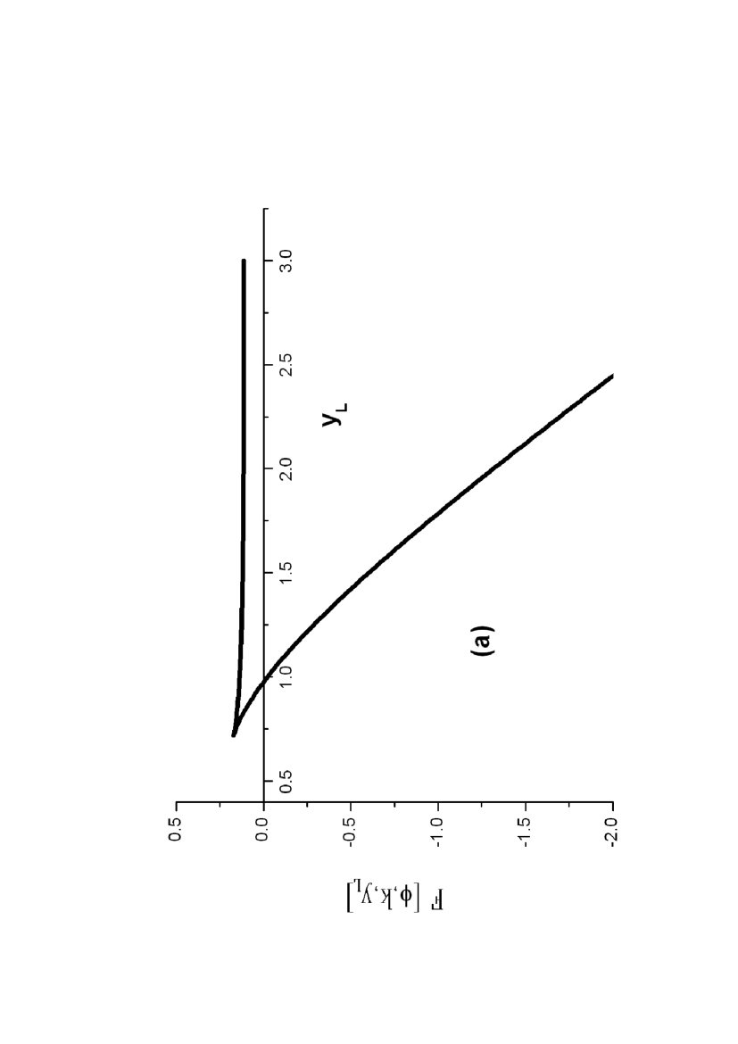
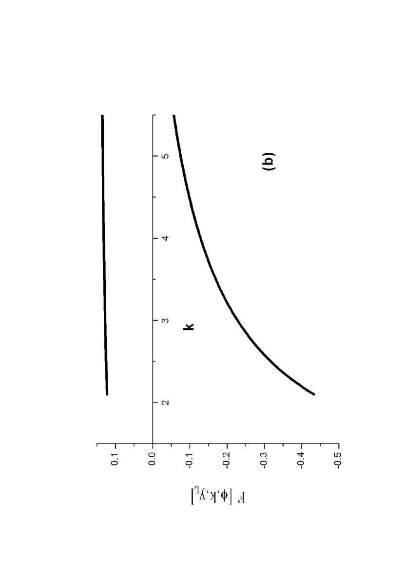
Figure 2: NEP $\mathcal{F}([\phi],k,y_{L})$ evaluated at the inhomogeneous stationary solutions $\phi_{1}(y)$ (lower branch) and $\phi_{u}(y)$ (upper branch), as a function of: (a) system’s size $y_{L}$, with $k=3.0$; (b) albedo parameter $k$, with $y_{L}=1.2$. The remaining parameters are $D=1.0$, $\phi_{c}/\phi_{h}=0.193$. The NEP for the homogeneous stationary solution $\phi_{0}(y)$ coincides with the horizontal axis.

One immediately notices that $\Delta\mathcal{F}^{1}(y_{L})\equiv\mathcal{F}^{u}(y_{L})-\mathcal{F}^{1}(y_{L})$ is an (almost linearly) increasing function of $y_{L}$ (this has a profound implication for SSSR, as we shall see below). Equation (3) has real solutions only for $y_{L}\gtrapprox 0.72$. This corresponds to a supercritical saddle–node bifurcation, at which both inhomogeneous structures pop up. Now, the most important feature in Fig. 2a is that $\mathcal{F}^{1}(y_{L})$ vanishes at a certain system’s size $y_{L}^{*}$ ($\approx 1.0$ for the given values of $k$ and $\phi_{c}/\phi_{h}$). At that point, the stable inhomogeneous structure $\phi_{1}(y)$ and the trivial solution $\phi_{0}(y)$ exchange their relative stabilities.

For completeness, in Fig. 2b we plot $\mathcal{F}([\phi],k)$ for the same value of $\phi_{c}/\phi_{h}$ as in Fig. 2a. For the chosen value of $y_{L}$ it is always $\mathcal{F}^{1}(k)<0$, and correspondingly there is no “stability exchange” as a function of $k$. Also, the initially large $\Delta\mathcal{F}^{1}(k)$ decreases with $k$ as $\mathcal{F}^{u}(k)$ and $\mathcal{F}^{1}(k)$ tend (for $k\to\infty$) to the values corresponding to Dirichlet’s b.c. IO .

2.2 Results for SSSR

By including an additive spatiotemporal noise source $\xi(y,t)$ extend3b ; nsp , Eq. (1) becomes a stochastic partial differential equation for the random field $\phi(y,t)$. The simplest assumptions about $\xi(y,t)$ are that it is Gaussian, with zero mean and a correlation function given by $\langle\xi(y,t)\xi(y^{\prime},t^{\prime})\rangle=2\gamma\,\delta(t-t^{\prime})\delta(y-y^{\prime})$, where $\gamma$ denotes the noise strength.

As discussed in extend2 ; extend2b ; extend3a ; extend3b , known results for activation processes in multidimensional systems HG allow us to estimate the activation rate using the following Kramers’-like expression for the mean first-passage time for the transitions between attractors

$$\langle\tau_{i}\rangle=\tau_{0}\,\exp\left[\frac{\Delta\mathcal{F}^{i}(y_{L})}{\gamma}\right],$$

where $\Delta\mathcal{F}^{i}(y_{L})=\mathcal{F}^{u}(y_{L})-\mathcal{F}^{i}(y_{L})$, $i=0,1$. The prefactor $\tau_{0}$ is usually determined by the curvature of $\mathcal{F}[\phi]$ at its extrema. On one hand, it is typically several orders of magnitude smaller than the average time $\langle\tau\rangle$, while on the other it does not change significatively when varying the system’s parameters around the “bistable point” $y_{L}^{*}$, where $\mathcal{F}([\phi_{0}],y_{L}^{*})=\mathcal{F}([\phi_{1}],y_{L}^{*})$. Hence we may simplify the analysis by assuming here that $\tau_{0}$ is constant, and scale it out of our results. The behavior of $\langle\tau\rangle$ as a function of $k$ and $\phi_{c}/\phi_{h}$ has been shown in extend2 ; extend2b ; IO .

As done in extend2 , we now assume that the system is (adiabatically) subject to an external harmonic variation of the parameter $\phi_{c}$: $\phi_{c}(t)=\phi_{c}^{0}+\delta\phi_{c}\cos(\omega t)$ extend2b ; extend3b , and exploit the “two-state approximation” RMP as in extend2b ; extend3a ; extend3b . Such approximation reduces the whole dynamics on the bistable potential landscape to one where the transitions occur only between the states associated to the bottom of each well, hence the only dynamical contents resides in the transition rates. Up to first order in the amplitude $\delta\phi_{c}$ (assumed to be small in order that the periodic input be sub-threshold) the transition rates $W_{i}$ adopt the form

$$W_{i}\simeq\frac{1}{2}\left[\mu_{i}\mp\alpha_{i}\frac{\delta\phi_{c}}{\gamma}\cos(\omega t)\right],$$ (5)

where (at constant $\phi_{h}$) $\mu_{i}\approx\exp[-\Delta\mathcal{F}^{i}(\phi_{c}^{0},y_{L})/\gamma]$ and $\alpha_{i}\approx\mu_{i}\,(\partial\Delta\mathcal{F}^{i}/\partial\phi_{c}|_{\phi_{c}^{0}})$, $i=0,1$. The quantity inside parentheses can be obtained analytically using Eq. (2.1). These results allow to calculate the autocorrelation function, the power spectrum density and finally the SNR, that we indicate by $R$. The detailed calculation can be found in the appendix of extend3a . Up to the relevant order (the second) in the signal amplitude $\delta\phi_{c}$, we obtain

$$R=\frac{\pi}{4\mu_{0}\mu_{1}}\,\frac{(\alpha_{0}\mu_{1}+\alpha_{1}\mu_{0})^{2}}{\mu_{0}+\mu_{1}}=\frac{\pi}{4\gamma^{2}}\,\frac{\mu_{0}\mu_{1}}{\mu_{0}+\mu_{1}}\,\Phi,$$ (6)

where we have used the form of the $\alpha_{i}$ to reduce the expression, and defined $\Phi=[2\phi_{h}\,y_{c}(y_{L})]^{2}$. Figure 3 (left) is a plot of $R$ as a function of the noise intensity $\gamma$ for a fixed system’s length $y_{L}$, displaying the typical maximum that has become the fingerprint of the SR phenomenon. In Fig. 3 (right), the roles of $\gamma$ and $y_{L}$ are exchanged ($R$ is plotted as a function of $y_{L}$ for fixed $\gamma$). Such a response is the expected one for a system exhibiting SSSR. In both cases, the values of $k$ and $\phi_{c}^{0}/\phi_{h}$ are kept fixed.

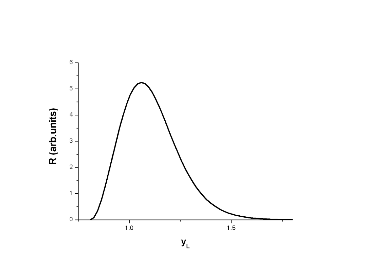
Figure 3: Left: SNR vs the noise intensity $\gamma$, with system’s size $y_{L}=1.1$. Right: SNR vs $y_{L}$, for $\gamma=0.1$. The remaining parameters are $k=3.0$, $D=1.0$, and $\phi_{c}^{0}/\phi_{h}=0.193$.

Within the NEP context and in this kind of systems, the phenomenon arises due to the breakdown of the NEP’s symmetry. This means that (as shown in Fig. 2) when varying $y_{L}$, both attractors can exchange their relative stability. For $y_{L}=y_{L}^{*}\approx 1$ both stable structures—the inhomogeneous one $\phi_{1}(y)$ and the trivial one $\phi_{0}$—have the same value for the NEP. For $y_{L}<y_{L}^{*}$, $\phi_{1}(y)$ becomes less stable than $\phi_{0}$ so transitions from $\phi_{1}(y)$ to $\phi_{0}$ are more frequent (the barrier is lower) than in the reverse direction, thus reducing the system’s response. When $y_{L}\sim 0.72$, $\phi_{1}(y)$ and $\phi_{u}(y)$ coalesce and disappear, and the response is strictly zero (within the linear response scheme implicit in the two-state approximation). When $y_{L}>y_{L}^{*}$, $\phi_{1}(y)$ becomes more stable than $\phi_{0}$, making now transitions from $\phi_{0}$ to $\phi_{1}(y)$ more frequent than in the reverse direction, and reducing again the system’s response. Clearly, the system’s response has a maximum when both attractors have the same stability ($y_{L}=y_{L}^{*}$), and decays when departing from that situation. Hence, for this system and within this framework, SSSR arises as a particular case of the more general discussion done in extend3a . It should not come as a surprise to find an analogy with the mechanism of double stochastic coherence described in sscr , where the NEP’s symmetry is induced by (an additional, multiplicative) noise.

By comparing figures 2a and 3 it becomes apparent that the value of $y_{L}$ at which the SNR has its maximum differs slightly from $y_{L}^{*}$ (where the crossing between $\mathcal{F}^{1}$ and $\mathcal{F}^{0}$ takes place). The origin of this discrepancy is the following: whereas on qualitative grounds we have argued that the maximum of the SNR should be related to the potential being symmetric (both wells having the same “energy”) extend3a , the exact condition is that the transition rates between both wells be equal. In general, due to small differences between the curvatures at the bottom of each well, those rates become equal for values of $y_{L}$ slightly different from the one at the symmetric case. Although by adopting here a constant value of $\tau_{0}$ we have assumed equal curvatures, there is still a difference in the values of the $\alpha_{i}$, since the $\partial\Delta\mathcal{F}^{i}/\partial\phi_{c}|_{\phi_{c}^{0}}$, $i=0,1$ are slightly different (a fact reflected in the dependence of $\Phi$ on $y_{L}$).

Additional light can be shed on the phenomenon when viewed from a different angle. Figure 4 is a plot of $R$ as a function of $k$ at fixed values of $\gamma$, $y_{L}$ and $\phi_{c}^{0}/\phi_{h}$. It exhibits a broad resonance since for $k$ not too large (indicating a high reflectiveness at the boundary or a reduced exchange with the environment) $R$ increases with $k$, whereas it slightly decreases for larger $k$ values (where the system’s boundaries become absorbent). An explanation of this behavior in terms of the NEP has been given in SSSR6 : as already observed, the NEP’s symmetry is broken for this value of $y_{L}$; moreover, whereas the lower branch in Fig. 2b goes rapidly towards the value corresponding to Dirichlet’s b.c. the upper branch keeps increasing, thus degrading the SNR. In any case, the fact that the resonance is broad indicates the robustness of the system’s response with regard to $k$, a parameter that (together with $\gamma$) encodes the coupling with the environment.

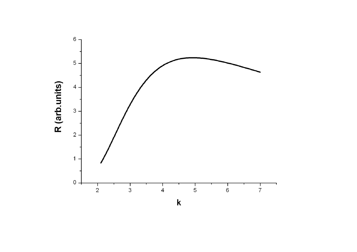
Figure 4: SNR vs $k$ for $y_{L}=1.2$, $\gamma=0.1$ and $\phi_{c}^{0}/\phi_{h}=0.193$.

We stress the fact that the NEP framework put forward in this review allows to study SSSR between whole patterns. The explanation offered in SSSR4 to the phenomenon resorted to a collective variable $X\approx(1/N)\sum_{j=1}^{N}x_{j}$, and to the fact that the noise in the effective stochastic differential equation for $X$ scaled with size. In SSSR6 it was shown that all the cases discussed in SSSR4 can be put within the same NEP framework than the above studied scalar model. In fact, the aforementioned almost linear increasing dependence of $\Delta\mathcal{F}^{1}(y_{L})$ on $y_{L}$ can be interpreted as a noise scaling with size. There are however situations where the NEP’s symmetry is retained as the system’s size is varied. We may then speak of a genuinely noise-scaling SSSR, in contrast to the cases that could be called NEP symmetry breaking SSSR SSSR6 .

3 Case of selective coupling

In this section we analyze SR in two extended systems with density-dependent diffusive-like coupling: an extension of the scalar RD model considered in Sec. 2 extend3c , and an array of FitzHugh–Nagumo FHN units.

3.1 Scalar model

Here we extend the one-component RD model discussed in Sec. 2 by letting the diffusive parameter $D$ in Eq. (1) depend on the field $\phi(x,t)$. As a matter of fact, since in the ballast resistor FHN ; SW the thermal conductivity is a function of the energy density, the resulting equation for the temperature field includes a temperature-dependent diffusion coefficient in a natural way. The form of the governing equation is now

$$\partial_{t}\phi(x,t)=\partial_{x}\left[D(\phi)\partial_{x}\phi\right]+f(\phi)+\xi(x,t),$$ (7)

with $\xi(x,t)$ and $f(\phi)$ as in Sec. 2.

As it was done for the reaction term, a simple choice (that retains however the qualitative features of the system) is to consider the following dependence of the diffusion term on the field variable

$$D(\phi)=D_{0}[1+h\,\Theta(\phi-\phi_{c})].$$

For simplicity, here we choose the same threshold $\phi_{c}$ for the reaction term and the diffusion coefficient.

We assume the system to lie in a bounded domain $[-L,L]$, with Dirichlet b.c. at both ends: $\phi(\pm L,t)=0$. The form of the patterns is analogous to what has been obtained in Sec. 2, the only difference being that in the present case $d\phi/dx|_{x_{c}}$ is discontinuous and the area of the “activated” central zone depends on $h$.

As before, the indicated patterns are extrema of the NEP: the unstable pattern $\phi_{u}(x)$ is a saddle-point of this functional, separating the attractors $\phi_{0}(x)$ and $\phi_{s}(x)$. For the case of a field-dependent diffusion coefficient $D(\phi(x,t))$ as described by Eq. (7), the NEP reads extend3c

$$\mathcal{F}[\phi]=\int_{-L}^{L}\left\{-\int_{0}^{\phi}D(\phi^{\prime})f(\phi^{\prime})\,d\phi^{\prime}+\frac{1}{2}\left[D(\phi)\frac{\partial\phi}{\partial x}\right]^{2}\,\right\}dx.$$

Given that $\partial_{t}\phi=-[1/D(\phi)](\delta\mathcal{F}/\delta\phi)$, one finds $d\mathcal{F}/dt=-\int(\delta\mathcal{F}/\delta\phi)^{2}\,dx\leq 0$, thus warranting the Lyapunov’s functional property.

Whereas in Sec. 2 we kept $\phi_{c}^{0}$ constant and varied $y_{L}$, we now vary instead $\phi_{c}^{0}$ at constant $L$. Similarly as before, both linearly stable states have the same value of the NEP (i.e., they are equally stable) at some value $\phi_{c}^{*}$ of the threshold. The way $\mathcal{F}[\phi]$ depends on $\phi_{c}^{0}$ resembles the dependence on $y_{L}$ shown in Sec. 2, but now $\Delta\mathcal{F}^{s}$ is an (almost linearly) decreasing function of $\phi_{c}^{0}$ and both inhomogeneous structures coalesce and disappear through a subcritical saddle–node bifurcation. As in the previous case, we analyze only the neighborhood of $\phi_{c}^{*}$. We shall moreover consider only the neighborhood of $h=0$, where the main trends of the effect can be captured.

Figure 5 (left) depicts the dependence of $R$ on the noise intensity $\gamma$ for three values of $h$, each curve displaying the typical SR maximum. Figure 5 (right) is a plot of the value $R_{\mathrm{max}}$ of these maxima as a function of $h$. The dramatic increase of $R_{\mathrm{max}}$ (several dB for a small positive variation of $h$) is apparent, and shows the strong effect that the selective coupling (or field-dependent diffusivity) has on the system’s response.

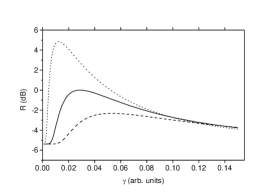
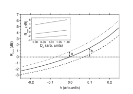
Figure 5: Left: SNR vs the noise intensity $\gamma$, for $D_{0}=1.0$ and $h=0.0$ (full line), $-0.25$ (dashed line) and 0.25 (dotted line). Right: the maximum $R_{\mathrm{max}}$ of the SNR curve as a function of the selectiveness $h$ of the coupling, for $D_{0}=0.9$ (dashed line), 1.0 (full line) and 1.1 (dotted line). The arrows a and b indicate the response gain due respectively to a homogeneous increase of the coupling and to a selective one. The larger gain in the second case is apparent. The inset shows the dependence of $R_{\mathrm{max}}$ on $D_{0}$ for $h=-0.25$ (lower line), 0.0 and 0.25 (upper line). The remaining parameters are $L=1.0$, $\delta\phi_{c}=0.01$ and $\Omega=0.01$.

It must be noted that the only two approximations made in order to derive our results—namely the Kramers-like expression and the two-level approximation used for the evaluation of the correlation function extend3c —break down for large positive values of $h$ because for increasing selectivity the curves of $\mathcal{F}[\phi]$ vs $\phi_{c}^{0}$ shift towards the left extend3c , which in turn means that the barrier separating the attractors at $\phi_{c}^{*}$ tends to zero. This effect is basically the same as the one discussed in Refs. extend2b ; extend3a in connection with global diffusivity $D_{0}$. It is also worth noting that except for the two aforementioned approximations, all the previous results (e.g. the profiles of the stationary patterns and the corresponding values of the nonequilibrium potential) are analytically exact.

3.2 FitzHugh–Nagumo model

Here we study an array of FitzHugh–Nagumo FHN units, with a density-dependent (diffusive-like) coupling. The NEP for this system was found within the excitable regime and for particular values of the coupling strength IO2 . In the general case, however, the form of the NEP has not been found yet. Hence, we have resorted to a study based on numerical simulations, analyzing the influence of different parameters on the system’s response. Nevertheless, the idea of the existence of such a NEP has always underlied this study. The results show that the enhancement of the SNR found for the scalar system extend3c is robust, and that the indicated non-homogeneous coupling could clearly contribute to enhance the SR phenomenon in more general situations.

We consider a simplified version of the FitzHugh–Nagumo model extend3c ; IO ; FHN , which has been useful for gaining qualitative insight into the excitable and oscillatory dynamics in neural and chemical systems. It consist of two variables:

• a (fast) activator field $u$, that in the case of neural systems represents the voltage variable, while in chemical systems represents the concentration of an autocatalytic species.

• an inhibitor field $v$, associated (within a neural context) to the concentration of potassium ions in the medium, and that in a general chemical reaction inhibits the generation of the $u$ species.

Instead of considering the usual cubic-like nonlinear form, we use a piecewise linear version

$$\epsilon\,\frac{\partial u(x,t)}{\partial t} = \frac{\partial}{\partial x}\left[D_{u}(u)\,\frac{\partial u}{\partial x}\right]+f(u)-v+\xi(x,t)$$ (8)

$$\frac{\partial v(x,t)}{\partial t} = \frac{\partial}{\partial x}\left[D_{v}(v)\,\frac{\partial u}{\partial x}\right]+\beta\,u-\alpha\,v,$$ (9)

where $f(u)=-u+\Theta(u-\phi_{c})$, and $\xi(x,t)$ is a $\delta$–correlated white Gaussian noise, as before. $\gamma$ indicates the noise intensity and $\phi_{c}$ is the “discontinuity” point, at which the piecewise linearized function $f(u)$ presents a jump. The parameter $\epsilon=\tau_{u}/\tau_{v}\ll 1$ indicates the timescale ratio between the (fast) activator and the inhibitor. Together with $\alpha$ and $\beta$, it is chosen to correspond to the excitable regime. We consider Dirichlet b.c. at $x=\pm L$. Although the results are qualitatively the same as those that could appear considering the usual FitzHugh–Nagumo equations, this simplified version allows us to compare directly with the previous analytical results for this system extend3c ; extend3b .

As in extend3c , we assume that the diffusion coefficient $D_{u}(u)$ is not constant, but depends on the field $u$ according to $D_{u}(u)=\,D_{u}^{0}\left[1+h\,\Theta(u-\phi_{c})\right]$. This form implies that the value of $D_{u}(u)$ depends “selectively” on whether the field $u$ fulfills $u>\phi_{c}$ or $u<\phi_{c}$. $D_{u}^{0}$ is the value of the diffusion constant without such “selective” term, and $h$ indicates the size of the difference between the diffusion constants in both regions [if $h=0$ then $D_{u}(u)=D_{u}^{0}$ constant]. $D_{v}(v)$ is the diffusion for the inhibitor $v$, that we assume to be homogeneously constant.

This system is known to exhibit two stable stationary patterns. One of them is $u(x)=0$, $v(x)=0$, while the other is one with nonzero values. Further, we consider, as before, that an external, periodic, signal enters into the system through the value of the threshold $\phi_{c}$, $\phi_{c}(t)=\phi_{c}^{0}+\delta\phi\,\cos(\omega t)$, where $\omega$ is the signal frequency, and $\delta\phi$ its intensity.

All the results were obtained through numerical simulations of the system. The continuous version of the system indicated by Eqs. (8), (9) was transformed into a second-order spatially discrete one

$$\dot{u_{i}} = D_{u_{i}}\Delta u_{i}+(D_{u_{i+1}}-D_{u_{i-1}})(u_{i+1}+u_{i-1})+f(u_{i})-v_{i}+\xi_{i}(t),$$

$$\dot{v_{i}} = D_{v}\Delta v_{i}+\beta\,u_{i}-\alpha\,v_{i},$$

with $\Delta\phi_{i}\equiv(\phi_{i-1}+\phi_{i+1}-2\phi_{i})$. The extensive numerical simulations performed for a set of equations were done exploiting Heun’s algorithm nsp .

In this spatially-extended system there are different ways of measuring the overall system’s response to the external signal. In particular, we show the evaluated output SNR in two different ways (the units being given in dB):

• SNR for the middle element of the chain evaluated over the dynamical evolution of $u_{N/2}$, that we call SNR₂ (however, having Dirichlet b.c., the local response depends on the distance to the boundaries).

• In order to measure the overall response of the system to the external signal, we computed the SNR as follows: We digitized the system’s dynamics to a dichotomic process $s(t)$: At time $t$ the system has an associated value of $s(t)=1\,(0)$ if the Hilbert distance to pattern $1\,(0)$ is lower than to the other pattern. Stated in mathematical terms, we computed the distance $\mathcal{D}_{2}[\cdot,\cdot]$ defined by

  $$\mathcal{D}_{2}[f,g]=\left\{\int_{-L}^{L}dx\,\left[f(x)-g(x)\right]^{2}\right\}^{1/2}$$

  in $\mathcal{L}^{2}([-L,L])$, the Hilbert space of the real-valued functions in that interval. At time $t$, a digitized process is computed by means of

  $$s(t)=\left\{\begin{array}[]{l}1\>\hbox{ if }\>\mathcal{D}_{2}\left[P^{u}_{1}(x),u(x,t)\right]<\mathcal{D}_{2}\left[P^{u}_{0}(x),u(x,t)\right]\\ 0\>\hbox{ if }\>\mathcal{D}_{2}\left[P^{u}_{1}(x),u(x,t)\right]\geq\mathcal{D}_{2}\left[P^{u}_{0}(x),u(x,t)\right]\end{array}\right.,$$

  We call this “global-like” measure SNR_p.

The parameters kept fixed have been summarized in Table 1. The simulation was repeated 250 times for each parameter set, and the SNR was computed by recourse of the average power spectral density.

Figure 6 depicts the results for the different SNR measures we have previously defined, as functions of the noise intensity $\gamma$. For both measures it is apparent that there is an enhancement of the response for $h>0$, when compared with the $h=0$ case, while for $h<0$ the response is smaller.

Model							Numerical
$\alpha$	$\beta$	$\epsilon$	$\phi_{c}^{0}$	$\delta\phi$	$\omega$	$D_{v}$	$\Delta t$	$N$
0.3	0.4	0.03	0.52	0.4	$5\pi/8$	1.0	$10^{-3}$	51

Table 1: Fixed parameters for the FitzHugh–Nagumo model with $D_{u}(u)$

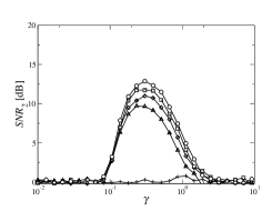
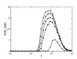
Figure 6: SNR₂ and SNR_p vs the noise intensity $\gamma$, for $D_{u}^{0}=0.3$ and $h=-2.0$ (+), $-1.0$ ($\triangle$), 0.0 ($\diamond$), 1.0 ($\square$), and 2.0 ($\bigcirc$). Both measures reveal a systematic enhancement of the SNR as $h$ increases.

In Fig. 7 we show again the response’s measures, but now as functions of $h$. We have plotted the maximum of each SNR curve for $D_{u}^{0}=0.3$, and $\gamma=0.01$, 0.1, and 0.3. It is clear that there exists an optimal value of $\gamma$ for which the response is largest. The rapid fall in the response for $h<0$ is also apparent.

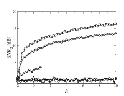
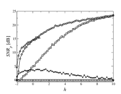
Figure 7: SNR₂ and SNR_p vs the selectiveness of coupling $h$, for $D_{u}^{0}=0.3$ and $\gamma=0.032$ ($\bigcirc$), 0.32 ($\square$), 0.6 ($\diamond$), 1.2 ($\triangle$), and 3.2 ($\times$).

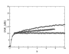
Figure 8: SNR₂ and SNR_p vs $h$ for $\gamma=0.032$ and $D_{u}^{0}=0.0$ ($\bigcirc$), 0.1 ($\square$), and 0.3 ($\diamond$).

In Fig. 8 we show the dependance of SNR on $h$, for different values of the diffusion which depends on the activator density $D_{u}^{0}$. It is apparent that the response becomes larger when the value of $D_{u}^{0}$ is larger. However, as was discussed in extend2 ; extend3b , it is clear that for still larger values of $D_{u}^{0}$, the symmetry of the underlying potential (that is the relative stability between the attractors) is broken and the response finally falls down.

The previous figures clearly show that the response to the external signal grows with the “selectiveness” of the coupling, showing the robustness of the phenomenon presented in extend3c ; extend3b .

4 Nonlocal Interaction

Let us consider again a system like the one described by Eqs. (8), (9), but now assume that $D_{u}$ and $D_{v}$ are constant. In Ref. IO1 it was assumed that the inhibitor-like field has a diffusive transport behavior, and is fast enough that can be adiabatically eliminated, thus yielding an effective scalar RD equation with a nonlocal term, characterized by a diffusive kernel $G(x,x^{\prime})$. After briefly reviewing the derivation of the NEP for that situation, we shall assume in this section that the transport mechanism of the adiabatically eliminated inhibitor-like field is of nondiffusive character, thus yielding a kernel $H(x,x^{\prime})$ that is more localized in space, and with a controllable interaction range.

Following Ref. IO1 , let the system be defined by

$$\partial_{t}u(x,t) = D_{u}\partial^{2}_{x}u(x,t)-u(x,t)+\Theta[u(x,t)-a]-v(x,t),$$

$$\epsilon^{-1}\,\partial_{t}v(x,t) = D_{v}\partial^{2}_{x}v(x,t)+\beta u(x,t)-\alpha v(x,t),$$ (10)

where $\epsilon$ was defined after Eqs. (8), (9), and let it be confined to the domain $[-L,L]$, with Dirichlet b.c. at both ends: $u(\pm L,t)=v(\pm L,t)=0$. Contrarily to the standard hypothesis, we now assume that the inhibitor is much faster than the activator (i.e. $\tau_{v}\ll\tau_{u}$). In the limit $\epsilon\to\infty$, we can rewrite Eq. (10) as

$$\partial_{t}u(x,t) = D_{u}\partial^{2}_{x}u(x,t)-u(x,t)+\Theta[u(x,t)-a]-v(x,t),$$

$$0 = D_{v}\partial^{2}_{x}v(x,t)+\beta u(x,t)-\alpha v(x,t).$$

In the last pair of equations we can eliminate the inhibitor (which is now slaved to the activator) by solving the second equation using the Green’s function method

$$[-D_{v}\partial^{2}_{x}+\alpha]\,G(x,x^{\prime}) = \delta(x-x^{\prime}),$$

$$v(x) = \beta\int dx^{\prime}G(x,x^{\prime})u(x^{\prime}),$$

where the Green’s function $G(x,x^{\prime})$ is given by

$$G(x,x^{\prime})=\frac{1}{D_{v}k}\left\{\begin{array}[]{lll}\left[\sinh k(L-x^{\prime})/\sinh 2kL\right]\sinh k(L+x)&&x<x^{\prime},\\ \left[\sinh k(L+x^{\prime})/\sinh 2kL\right]\sinh k(L-x)&&x>x^{\prime},\\ \end{array}\right.$$

with $k=(\alpha/D_{v})^{1/2}$. This slaving procedure reduces our system to a nonlocal equation for the activator only, that has the form

$$\frac{\partial u(x,t)}{\partial t}=D_{u}\,\frac{\partial^{2}u(x,t)}{\partial x^{2}}+f(u)-\beta\int_{-L}^{L}G(x,x^{\prime})\,u(x^{\prime})\,dx^{\prime}.$$ (11)

From this equation, and taking into account the symmetry of the Green’s function $G(x,x^{\prime})$, we can obtain the Lyapunov functional for this system, which has the form

$$\mathcal{F}[u]=\int_{-L}^{L}dx\left[\frac{D_{u}}{2}\left(\frac{\partial u}{\partial x}\right)^{2}-\int^{u}f(w)\,dw+\frac{\beta}{2}\int_{-L}^{L}dx^{\prime}\,G(x,x^{\prime})\,u(x^{\prime})\,u(x)\right].$$ (12)

This spatial nonlocal term in the NEP takes into account the repulsion between activated zones. When two activated zones come near each other, the exponential tails of the inhibitor concentration overlap, increasing its concentration between both activated zones and creating an effective repulsion between them. Hence the Green’s function plays the role of an exponential screening between the activated zones. In Ref. extend2b the knowledge of such NEP was exploited to study SR on the system indicated by Eq. (11).

The starting point of our present analysis will be the effective, nonlocal and stochastic RD equation for the real (activator-like) field $\phi(x,t)$, analogous to Eq. (11), defined in the one dimensional domain $x\in[-L,L]$ by

$$\frac{\partial\phi}{\partial t}=D\,\frac{\partial^{2}\phi}{\partial x^{2}}+f(\phi)-\beta\int_{-L}^{L}H(x,x^{\prime})\,\phi(x^{\prime})\,dx^{\prime}+\xi(x,t),$$

where the diffusivity $D$ is constant, and we assume a cubic nonlinear term $f(\phi)=\phi\,(\phi-b)\,(2-\phi)$. Here $\xi(x,t)$ is an additive Gaussian white noise, as in the previous cases. As before, the system is subject to Dirichlet b.c. $\phi(\pm L,t)=0$.

Similarly to Eq. (11), this system could be written in a variational form, with the functional $\mathcal{F}[\phi]$ given by Eq. (12). As anticipated, here we consider a nondiffusive kernel, with a controllable interaction range. In order to keep our analysis simple we propose the following form

$$H(x,x^{\prime})=\left\{\begin{array}[]{cl}1/2;&|x-x^{\prime}|\leq l\\ 0;&|x-x^{\prime}|>l,\end{array}\right.$$ (13)

which allows the analysis by just varying the interaction range $2l$.

The new effective RD equation contains local and nonlocal couplings (corresponding to the diffusive and the nonlocal contribution, respectively). The last one contains the nonlocal kernel given by Eq. (13), with a variable range $2l$, that corresponds to the interaction of the field at points $x^{\prime}\in[x-l,x+l]$. However, such points will contribute if and only if they are inside the domain $[-L,L]$. We are now in position to study the role played by the nonlocal kernel (particularly by its range $2l$) on the SR phenomenon.

As before, the SR between stationary solutions was investigated in terms of the two-state approach (all the details about the procedure and the evaluation of the SNR can be found in Refs. extend3a ; extend3b ). As usual, we subject our system to a weak external signal $b=b_{0}+A(t)=b_{0}+\Delta b\,\cos(\omega_{s}t)$, rocking the NEP extend3b . In order to have a subthreshold signal, the amplitude $\Delta b$ should satisfy $\Delta b\ll b$. We have chosen $b_{0}$ as the value of $b$ at which $\mathcal{F}[\phi_{s}]=\mathcal{F}[\phi=0]=0$ when $\beta=0$.

Up to first order in the small amplitude $\Delta b$, the transition rates $W_{i}$ and the functions $\alpha_{i}$ have the form indicated in Eqs. (5), (6). But now $\Phi$, that depends on the inhomogeneous attractor $\phi_{s}$, has the form

$$\Phi=\left[\int_{-L}^{L}\phi_{s}^{2}\left(1-\frac{\phi_{s}}{3}\right)dx\right]^{2}.$$

After fixing the length of the system $L$ and the kernel range $2l$ we can use the above indicated expressions to find the SNR, that shows the usual bell-shaped form of stochastic resonance as a function of the noise intensity.

In Fig. 9 we show the dependence of the SNR on the kernel range $2l$ for a fixed value of $2L$. There is a nonmonotonic behavior in the system’s response against variation of $2l$, that can be explained by the following facts:

• On one hand, the transition rates are decreasing functions of the range $2l$ for fixed $2L$. Therefore, the ratio $\mu_{1}\mu_{2}/(\mu_{1}+\mu_{2})$ in the expression for the SNR also reflects this behavior.

• The other factor in this expression has a maximum for a kernel range that corresponds to “first neighbor” sites, namely $x=x^{\prime}\pm l$.

Figure 9: SNR as a function of $2l$ for $2L$ fixed. The parameters are $D=0.6$, $2L=6.25$, $\beta=0.02$ and $b_{0}=0.719123$.

The maximum in the system’s response as a function of the kernel range is due to the interplay between these two factors. From this analysis of the comparative weights of the local (diffusive) and nonlocal terms contributing to the SR response, it is apparent that the range of such nonlocal kernel has an optimum value yielding a maximum for the SNR bvhhswnew .

5 Conclusions

We have discussed three different aspects of the phenomenon of stochastic resonance in reaction–diffusion systems, within the nonequilibrium potential’s framework. In first place we have discussed system-size SR in a scalar model. Even though we have not shown the details here, it has been also possible to also study other cases SSSR6 . In particular, a model of globally coupled nonlinear oscillators discussed in SSSR4 , showing that it can also be described within the NEP framework, with SSSR arising through an “effective” scaling of the noise intensity with the system’s size.

In second place we presented a study of SR in systems with a density-dependent (diffusive-like) coupling. We initially discuss the case of a scalar system extend3c , and afterwards extent the analysis to an array of FitzHugh–Nagumo units, with a field-dependent activator diffusion TW . For the second system, when both diffusions are constant (that is: $D_{u}>0$ and $D_{v}=0$), has a known form of the NEP extend3b . However, in the general case we have not been able to find the form of the NEP (but the idea of such a NEP is always underlying our analysis) and have to resort to an analysis based on numerical simulations. The result shows that the system’s response is enhanced due to the particular form of the non-homogeneous coupling. From such results, we can conclude that the phenomenon of enhancement of the SNR, due to a selectivity in the coupling, initially found for a scalar system extend3c is robust, and that the indicated non-homogeneous coupling could clearly contribute to enhance the SR phenomenon in very general systems.

Finally, we analyzed an activator-like field including a nonlocal contribution that arise through an effective adiabatic elimination of an auxiliary (inhibitor-like) field. By exploiting the knowledge of the nonequilibrium potential in such a case, we have analyzed the dependence of the SNR on the nonlocal interaction kernel range, founding that there is an optimal value of the kernel range, yielding a maximum in the system’s response, corresponding to a very localized interaction.

The indicated results clearly show that the “nonequilibrium potential” (even if not known in detail quasi ) offers a very useful framework to analyze a wide spectrum of characteristics associated to SR in spatially extended or coupled systems. For instance, within this framework, the phenomenon of SSSR looks—as other aspects of SR in extended systems extend3a —as a natural consequence of a breaking of the symmetry of the NEP SSSR4 .

Appendix: Brief review of the nonequilibrium potential scheme

Loosely speaking, the notion of NEP is an extension to nonequilibrium situations of that of equilibrium thermodynamic potential. In order to introduce it, we consider a general system of nonlinear stochastic equations (admitting the possibility of multiplicative noises)

$$\dot{q}^{\nu}=K^{\nu}(q)+g^{\nu}_{i}(q)\,\xi_{i}(t),\qquad\nu=1,\ldots,n;$$ (14)

where repeated indices are summed over. Equation (14) is stated in the sense of Itô. The $\{\xi_{i}(t)\}$, $i=1,\ldots,m\leq n$ are mutually independent sources of Gaussian white noise with typical strength $\gamma$.

Graham’s approach

The Fokker–Planck equation corresponding to Eq. (14) takes the form

$$\frac{\partial P}{\partial t}=-\frac{\partial}{\partial q^{\nu}}\,K^{\nu}(q)\,P+\frac{\gamma}{2}\frac{\partial^{2}}{\partial q^{\nu}\,\partial q^{\mu}}\,Q^{\nu\mu}(q)\,P$$ (15)

where $P(q,t;\gamma)$ is the probability density of observing $q=(q_{1},\ldots,q_{n})$ at time $t$ for noise intensity $\gamma$, and $Q^{\nu\mu}(q)=g^{\nu}_{i}(q)\,g^{\mu}_{i}(q)$ is the matrix of transport coefficients of the system, which is symmetric and non-negative. In the long time limit ($t\to\infty$), the solution of Eq. (15) tends to the stationary distribution $P_{\mathrm{st}}(q)$. According to GR , the NEP $\Phi(q)$ associated to Eq. (15) is defined by

$$\Phi(q)=-\lim_{\gamma\to 0}\gamma\,\ln P_{\mathrm{st}}(q,\gamma).$$ (16)

In other words

$$P_{\mathrm{st}}(q)\,d^{n}q=Z(q)\exp\left[-\frac{\Phi(q)}{\gamma}+\mathcal{O}(\gamma)\right]\,d\Omega_{q},$$

where $\Phi(q)$ is the NEP of the system and $Z(q)$ is defined as the limit

$$\ln Z(q)=\lim_{\gamma\to 0}\left[\ln P_{\mathrm{st}}(q,\gamma)+\frac{1}{\gamma}\,\Phi(q)\right].$$

Here $d\Omega_{q}=d^{n}q/\sqrt{G(q)}$ is the invariant volume element in the $q$-space and $G(q)$ is the determinant of the contravariant metric tensor (for the Euclidean metric it is $G=1$). It was shown GR that $\Phi(q)$ is the solution of a Hamilton–Jacobi-like equation (HJE)

$$K^{\nu}(q)\frac{\partial\Phi}{\partial q^{\nu}}+\frac{1}{2}Q^{\nu\mu}(q)\frac{\partial\Phi}{\partial q^{\nu}}\frac{\partial\Phi}{\partial q^{\mu}}=0,$$

and $Z(q)$ is the solution of a linear first-order partial differential equation depending on $\Phi(q)$ (not shown here).

Equation (16) and the normalization condition ensure that $\Phi$ is bounded from below. Furthermore, from the separation of the streaming velocity of the probability flow in the steady state into conservative and dissipative parts, it follows that

$$\frac{d\Phi(q)}{dt}=K^{\nu}(q)\frac{\partial\Phi(q)}{\partial q^{\nu}}=-\frac{1}{2}\,Q^{\nu\mu}(q)\,\frac{\partial\Phi}{\partial q^{\nu}}\frac{\partial\Phi}{\partial q^{\mu}}\leq 0,$$

i.e. $\Phi$ is a LF for the dynamics of the system when fluctuations are neglected. Under the deterministic dynamics, $\dot{q}^{\nu}=K^{\nu}(q)$, $\Phi$ decreases monotonically and takes a minimum value on attractors. In particular, $\Phi$ must be constant on all extended attractors (such as limit cycles or strange attractors) GR .

Ao’s approach

An alternative way to look into this problem is due to Ao pao . Let us refer again to the system in Eq. (14). Following pao , we introduce now the auxiliary matrix

$$\mathbf{H}^{-1}(\vec{q})=\mathbf{S}(\vec{q})+\mathbf{A}(\vec{q}),$$

with $\mathbf{S}(\vec{q})$ a symmetric matrix while $\mathbf{A}(\vec{a})$ is an antisymmetric one. $\mathbf{H}^{-1}(\vec{q})$ is now used to rewrite the initial system as

$$\mathbf{H}^{-1}(\vec{q})\,\dot{\vec{q}}=\mathbf{H}^{-1}(\vec{q})\,\vec{K}(\vec{q},t)+\mathbf{H}^{-1}(\vec{q})\,\vec{\xi}(\vec{q},t)=-\nabla\Phi(\vec{q},t)+\vec{\eta}(\vec{q},t),$$

where $-\nabla\Phi(\vec{q},t)=\mathbf{H}^{-1}(\vec{q})\,\vec{K}(\vec{q},t)$, $\vec{\eta}(\vec{q},t)=\mathbf{H}^{-1}(\vec{q})\,\vec{\xi}(\vec{q},t)$ and $\mathbf{H}^{-1}(\vec{q})\,\dot{\vec{q}}=-\nabla\Phi(\vec{q},t)+\vec{\eta}(\vec{q},t)$. The new stochastic variables, $\vec{\eta}(\vec{q},t)$, fulfill

$$\langle\vec{\eta}(\vec{q},t)\vec{\eta}^{T}(\vec{q},t^{\prime})\rangle=2\,\mathbf{S}(\vec{q})\,\delta(t-t^{\prime})=2\,\mathbf{G}^{-1}(\vec{q})\mathbf{Q}(\vec{q})[\mathbf{G}^{-1}(\vec{q})]^{T}\delta(t-t^{\prime}),$$

that imposes a condition on the arbitrary definition of $\mathbf{S}(\vec{q})$ as we have

$$[\mathbf{S}(\vec{q})+\mathbf{A}(\vec{q})]\,\mathbf{Q}(\vec{q})\,[\mathbf{S}(\vec{q})-\mathbf{A}(\vec{q})]=\mathbf{S}(\vec{q}).$$

As shown by Ao, the last equation also implies $\mathbf{H}(\vec{q})+\mathbf{H}^{T}(\vec{q})=2\,\mathbf{Q}(\vec{q})$. We also have $\nabla\times\left[\mathbf{H}^{-1}(\vec{q})\,\vec{K}(\vec{q},t)\right]=\nabla\times\left[-\nabla\Phi(\vec{q},t)\right]=0$. From the previous equations, we have in principle all the needed conditions to determine $\mathbf{H}^{-1}(\vec{q})$, and to obtain from it the potential $\Phi(\vec{q},t)$. The interesting feature of this approach is that it resorts neither to $P_{\mathrm{st}}(q)$ nor to the small-noise limit, thus being applicable in principle to more general situations.

References

- (1) L. Gammaitoni, P. Hänggi, P. Jung, and F. Marchesoni, Rev. Mod. Phys. 70, 223 (1998).
- (2) T. Wellens, V. Shatokin, and A. Buchleitner, Rep. Prog. Phys. 67, 45 (2004).
- (3) A. S. Pikovsky and J. Kurths, Phys. Rev. Lett. 78, 775 (1997).
- (4) J. K. Douglas et al., Nature 365, 337 (1993); J. J. Collins et al., Nature 376, 236 (1995); S. M. Bezrukov and I. Vodyanoy, Nature 378, 362 (1995).
- (5) A. Guderian, G. Dechert, K. Zeyer, and F. Schneider, J. Phys. Chem. 100, 4437 (1996); A. Förster, M. Merget, and F. Schneider, J. Phys. Chem. 100, 4442 (1996); W. Hohmann, J. Müller, and F. W. Schneider; J. Phys. Chem. 100, 5388 (1996).
- (6) J. F. Lindner et al., Phys. Rev. E 53, 2081 (1996).
- (7) A. R. Bulsara and G. Schmera, Phys. Rev. E 47, 3734 (1993); P. Jung, U. Behn, E. Pantazelou, and F. Moss, Phys. Rev. A 46, R1709 (1992); P. Jung and G. Mayer-Kress, Phys. Rev. Lett. 74, 2130 (1995); J. F. Lindner et al., Phys. Rev. Lett. 75, 3 (1995); F. Marchesoni, L. Gammaitoni, and A. R. Bulsara, Phys. Rev. Lett. 76, 2609 (1996).
- (8) H. S. Wio, Phys. Rev. E 54, R3075 (1996); H. S. Wio and F. Castelpoggi, Unsolved Problems of Noise, Proc. Conf. UPoN’96, C. R. Doering, L. B. Kiss, and M. Schlesinger, Eds. (World Scientific, Singapore, 1997), pg. 229; F. Castelpoggi and H. S. Wio, Europhys. Lett. 38, 91 (1997).
- (9) F. Castelpoggi and H. S. Wio, Phys. Rev. E 57, 5112 (1998).
- (10) H. S. Wio et al., Physica A 257, 275 (1998); M. Kuperman, H. S. Wio, G. Izús, and R. Deza, Phys. Rev. E 57, 5122 (1998).
- (11) S. Bouzat and H. S. Wio, Phys. Rev. E 59, 5142 (1999).
- (12) B. von Haeften, R. Deza, and H. S. Wio, Phys. Rev. Lett. 84, 404 (2000).
- (13) C. J. Tessone, H. S. Wio, and P. Hänggi, Phys. Rev. E 62, 4623 (2000).
- (14) M. A. Fuentes, R. Toral, and H. S. Wio, Physica A 295, 114 (2001).
- (15) H. S. Wio, S. Bouzat and B. von Haeften, in Proc. 21st IUPAP Int. Conf. on Statistical Physics, STATPHYS21, A. Robledo and M. Barbosa (Eds.), Physica A 306C, 140-156 (2002).
- (16) R. Graham, in Instabilities and Nonequilibrium Structures, Eds. E. Tirapegui and D. Villaroel (D. Reidel, Dordrecht, 1987); R. Graham and T. Tél, Phys. Rev. A 42, 4661 (1990); R. Graham and T. Tél, in Instabilities and Nonequilibrium Structures III, E. Tirapegui and W. Zeller, eds. (Kluwert, 1991); O. Descalzi and R. Graham, Phys. Lett. A 170, 84 (1992); O. Descalzi and R. Graham, Z. Phys. B 93, 509 (1994); H. S. Wio, in 4th Granada Seminar in Computational Physics, Eds. P. Garrido and J. Marro (Springer-Verlag, Berlin, 1997), pg.135.
- (17) G. Izús et al., Phys. Rev. E 52, 129 (1995); G. Izús et al., Int. J. Mod. Phys. B 10, 1273 (1996).
- (18) G. Drazer and H. S. Wio, Physica A 240, 571 (1997).
- (19) D. H. Zanette, H. S. Wio and R. Deza, Phys. Rev. E 53, 353 (1996); F. Castelpoggi, H. S. Wio and D. H. Zanette, Int. J. Mod. Phys. B 11, 1717 (1997); G. Izús, R. Deza and H. S. Wio, Phys. Rev. E 58, 93 (1998); S. Bouzat and H. S. Wio, Phys. Lett. A 247, 297 (1998); G. G. Izús, R. R. Deza and H. S. Wio, Comp. Phys. Comm. 121-122, 406 (1999).
- (20) B. von Haeften et al., Phys. Rev. E 69, 021107 (2004); B. von Haeften et al., in Noise in Complex Systems and Stochastic Dynamics, Z. Gingl, J. M. Sancho, L. Schimansky-Geier, and J. Kerstez (Eds.), Proc. SPIE 5471, 258-265 (2004).
- (21) H. S. Wio, in Noise and Fluctuations, Proc. 18th Int. Conf. on Noise and Fluctuations-ICNF2005, Eds. T. Gonzalez, J. Mateos, D. Pardo, AIP 780, 55 (2005).
- (22) C. J. Tessone and H. S. Wio, Physica A 374, 46 (2006).
- (23) H. S. Wio, An Introduction to Stochastic Processes and Nonequilibrium Statistical Physics (World Scientific, Singapore, 1994); A. S. Mikhailov, Foundations of Synergetics I (Springer-Verlag, Berlin, 1990).
- (24) G. Schmid, I. Goychuk, and P. Hänggi, Europhys. Lett. 56, 22 (2001); ibid., Phys. Biol. 1, 61 (2004).
- (25) P. Jung and J. W. Shuai, Europhys. Lett. 56, 29 (2001); J. W. Shuai and P. Jung, Phys. Rev. Lett. 88, 068102 (2003).
- (26) R. Toral, C. Mirasso, and J. Gunton, Europhys. Lett. 61, 162 (2003).
- (27) A. Pikovsky, A. Zaikin, and M. A. de la Casa, Phys. Rev. Lett. 88, 050601 (2002).
- (28) C. J. Tessone and R. Toral, Physica A 351, 106-116 (2005).
- (29) B. von Haeften, G. G. Izús, and H. S. Wio, Phys. Rev. E 72, 021101 (2005).
- (30) C. L. Schat and H. S. Wio, Physica A 180, 295 (1992).
- (31) P. Hänggi, P. Talkner, and M. Borkovec, Rev. Mod. Phys. 62, 251 (1990).
- (32) A. Zaikin et al., Phys. Rev. Lett. 90, 030601 (2003).
- (33) J. García-Ojalvo and J. M. Sancho, Noise in Spatially Extended Systems (Springer-Verlag, New York, 1999).
- (34) It is worthwhile noting that when the parameter is large enough, under some circumstances the coupling term might become negative, in what is known as “inhibitory coupling” Dayan . This is a very interesting kind of coupling that has attracted much attention, both in neural and chemical context, that we will not discuss here.
- (35) P. Dayan and L. F. Abbott, Theoretical neuroscience: Computational and mathematical modeling of neural systems (MIT Press, Cambridge, 2001).
- (36) B. von Haeften and H. S. Wio, Physica A 376, 199 (2007).
- (37) P. Ao, cond-mat/0302081 (2003); P. Ao, J. Phys. A 37, L25-L30 (2004).