The VLT-FLAMES survey of massive stars:
Wind properties and evolution of hot massive stars in the LMC

We have studied the optical spectra of a sample of 28 O- and early B-type stars in the Large Magellanic Cloud, 22 of which are associated with the young star forming region N11. Our observations sample the central associations of LH9 and LH10, and the surrounding regions. Stellar parameters are determined using an automated fitting method (Mokiem et al. 2005), which combines the stellar atmosphere code fastwind (Puls et al. 2005) with the genetic algorithm based optimisation routine pikaia (Charbonneau 1995). We derive an age of $7.0\pm 1.0$ and $3.0\pm 1.0$ Myr for LH9 and LH10, respectively. The age difference and relative distance of the associations are consistent with a sequential star formation scenario in which stellar activity in LH9 triggered the formation of LH10. Our sample contains four stars of spectral type O2. From helium and hydrogen line fitting we find the hottest three of these stars to be $\sim$$49-54$ kK (compared to $\sim$$45-46$ kK for O3 stars). Detailed determination of the helium mass fraction reveals that the masses of helium enriched dwarfs and giants derived in our spectroscopic analysis are systematically lower than those implied by non-rotating evolutionary tracks. We interpret this as evidence for efficient rotationally enhanced mixing leading to the surfacing of primary helium and to an increase of the stellar luminosity. This result is consistent with findings for SMC stars by Mokiem et al. (2006). For bright giants and supergiants no such mass discrepancy is found; these stars therefore appear to follow tracks of modestly or non-rotating objects. The set of programme stars was sufficiently large to establish the mass loss rates of OB stars in this $Z\sim 1/2\,\mbox{$Z_{\sun}$}$ environment sufficiently accurate to allow for a quantitative comparison with similar objects in the Galaxy and the SMC. The mass loss properties are found to be intermediate to massive stars in the Galaxy and SMC. Comparing the derived modified wind momenta $D_{\rm mom}$ as a function of luminosity with predictions for LMC metallicities by Vink et al. (2001) yields good agreement in the entire luminosity range that was investigated, i.e. $5.0<\log L/\mbox{$L_{\sun}$}<6.1$.

1 Introduction

Massive stars play an intricate role in the evolution of galaxies. Because of the large energies associated with their stellar winds, ionising radiation, and life-ending supernova explosions, they dictate galactic structuring processes such as star formation and the creation and evolution of supperbubbles (e.g. Oey 1999). Mounting evidence also points to a direct link between massive stars and exotic phenomena such as $\gamma$-ray bursts (e.g. Hjorth et al. 2003) and the reionisation of the early universe (Bromm et al. 2001). Accordingly, understanding the properties of these stars, both in terms of their fundamental parameters as well as their evolution, is fundamental.

The initial metal composition ($Z$) of the gas out of which massive stars form has a strong impact on their global properties and characteristics. Many studies have shown that parameters such as the effective temperature and ionising fluxes are strong functions of $Z$ (e.g. Kudritzki 2002; Mokiem et al. 2004; Massey et al. 2005; Mokiem et al. 2006), adding an extra dimension to the conversion of morphological properties such as spectral type to physical quantities. Theoretical and observational arguments (e.g. Kudritzki & Puls 2000; Vink et al. 2001) also point to a relation between the strengths of the stellar winds of these objects and metallicity. As wind mass loss leads to partial evaporation of the star (e.g. Chiosi & Maeder 1986) – with possible consequences for the nature of the compact object that is left behind after the final supernova explosion – and to loss of angular momentum (e.g. Meynet & Maeder 2000), it also dictates to a large extent its evolutionary path and fate (e.g. Yoon & Langer 2005; Woosley & Heger 2006). Quantifying the mass loss versus metallicity dependence $\mbox{$\dot{M}$}(Z)$, therefore, is an important quest in astrophysics.

Due to their proximity and low metal content the Magellanic Clouds provide us with unparallelled laboratories to test and enlarge our knowledge of massive stars. These galaxies, therefore, have been in the focal point of many studies analysing their massive star content. Early studies (e.g. Conti et al. 1986; Garmany et al. 1987; Massey et al. 1989; Parker et al. 1992; Walborn et al. 1999) predominantly relied on photometric data and spectral type calibrations. Only relatively recent the advent of large telescopes and the development of sophisticated stellar atmosphere models has allowed for more detailed analyses of individual stars (e.g. Puls et al. 1996; Hillier & Miller 1999; Crowther et al. 2002; Bouret et al. 2003; Martins et al. 2004). Though all these studies have contributed enormously to our understanding of massive stars, the samples analysed so far have been rather limited in size (a few objects at a time) and have been focused predominantly on objects in the Small Magellanic Cloud (SMC) – because its metal deficiency is more extreme than that of the Large Magellanic Cloud (LMC) (but see Massey et al. 2004, 2005).

The limited sizes of the samples that have so far been studied are at the root cause of the perhaps somewhat disheartening conclusion that – in spite of all the progress that has been made – we still cannot provide robust and sound answers to the question: what is the role of metal content, stellar winds and rotation in the evolution of massive stars? To help attack this problem, our research group has conducted a VLT-FLAMES Survey of Massive Stars (see Evans et al. 2005). In this ESO Large Program the Fibre Large Array Multi-Element Spectrograph at the Very Large Telescope was used to obtain optical spectra of more than 50 O- and early B-type stars in the Magellanic Clouds.

Here we present the homogeneous analysis, employing automated spectral fitting methods, of a sample of 28 O-type and early B-type stars in the Large Magellanic Cloud; 22 targets from the FLAMES survey and 6 from other sources. This is so far the largest sample of massive stars studied in the LMC and it almost doubles the amount of massive objects in this galaxy for which parameters have been derived from quantitative spectroscopy. Specifically, we will try to establish the mass loss rates of OB stars in this $Z\sim 1/2\,\mbox{$Z_{\sun}$}$ environment to a level of precision that allows for a quantitative comparison with similar objects in the SMC and our Galaxy. This will provide a new $Z$-point in testing the fundamental prediction provided by radiation driven wind theory for the mass-loss – metallicity dependence: $\mbox{$\dot{M}$}(Z)\propto Z^{0.5-0.7}$ (e.g. Kudritzki et al. 1987; Puls et al. 2000; Vink et al. 2001).

The majority of our LMC sample is associated with the spectacular star forming region N11 (Henize 1956). It has a H$\alpha$ luminosity only surpassed by that of 30 Doradus (Kennicutt & Hodge 1986), ranking it as the second largest H ii region in the Magellanic Clouds. N11 is host to several OB associations of apparently different ages, the formation of which is believed to have been triggered by stellar activity in the central OB cluster (Parker et al. 1992; Walborn & Parker 1992; Walborn et al. 1999). Our observations sample both the central cluster LH9 as well as the younger cluster LH10, allowing for an investigation of a possible sequential star formation scenario. We will use our N11 stars to test predictions of massive star evolution, including the role of rotation, and the star formation history.

This paper is organised as follows: in Sect. 2 we describe the LMC data set that was analysed using our automated genetic algorithm based fitting method. A short description of this method is given in Sect. 3 and the results obtained are presented in Sect. 4, with fits and comments on individual objects given in the appendix. In Sect. 5 we investigate the discrepancy between spectroscopically determined masses and those derived from evolutionary tracks. The evolutionary status of N11 is discussed in Sect. 6. Finally, Sect. 7 summarises and lists our most important findings.

2 Data description

Our OB-type star sample is mainly drawn from the targets observed in the LMC within the context of the VLT-FLAMES survey of massive stars (see Evans et al. 2005). Two fields in the LMC centred on the clusters N11 and NGC 2004 were observed in the survey. Here we analyse a subset of the objects observed in the N11 field. This set consists of all O-type spectra obtained, excluding those that correspond to confirmed binaries, and five early B-type spectra of luminous giant and supergiant stars.

To improve the sampling in luminosity and temperature, we supplemented the FLAMES targets with six relatively bright O-type field stars. These objects are part of the Sanduleak (1970, hereafter Sk) and Brunet et al. (1975, hereafter BI) catalogues, and were observed as part of the programs 67.D-0238, 70.D-0164 and 074.D-0109 (P.I. Crowther) using the Ultraviolet and Visual Echelle Spectrograph (UVES) at the VLT.

The observations of the FLAMES targets are described extensively by Evans et al. (2006), to which we refer for full details. Here we only summarise the most important observational parameters. Basic observational properties of the programme stars together with common aliases are given in Tab. 1. Note that N11-031, BI 237, BI 253 and Sk$-67$ 166 were studied recently using line blanketed stellar atmosphere models. In the appendix a comparison with these analyses is provided. The FLAMES targets were observed with the Giraffe spectrograph mounted at UT2. For six wavelength settings a spectrum was acquired six times for each object with an effective resolving power of $R\simeq 20\,000$. These multiple exposures, often at different epochs, allowed for the detection of variable radial velocities. As a result, a considerable number of binaries could be detected (Evans et al. 2006), which we subsequently excluded from our analysis.

Table 1: Basic parameters. Primary identification numbers for N11 are from Evans et al. (2006). Identifications starting with “Sk”, “PGMW” and “BI” are from, respectively, Sanduleak (1970), Parker et al. (1992) and Brunet et al. (1975). Photometric data for these objects are from Evans et al. (2006) and Parker et al. (1992), the latter are flagged with an asterisk. For non-N11 objects these are from Ardeberg et al. (1972), Issersted (1979) and Massey (2002). Wind velocities given without brackets are from Crowther et al. (2002), Massa et al. (2003) and Massey et al. (2005). For Sk $-66$ 18 the wind velocity was measured from O iv (1031-1037 Å) in its FUSE spectrum. Values between brackets are calculated from the escape velocity at the stellar surface. For N11-031 the value of $v_{\infty}$ is from Walborn et al. (2004), though this is actually based on the value obtained for Sk-68 137 by Prinja & Crowther (1998).

Primary ID	Cross-IDs	Spectral	$V$	$A_{V}$	$M_{V}$	$v_{\infty}$
		Type				[km s-1]
N11-004	Sk $-66$ 16	OC9.7 Ib	12.56	0.74	$-6.68$	[2387]
N11-008	Sk $-66$ 15	B0.7 Ia	12.77	0.84	$-6.57$	[1619]
N11-026	…	O2 III(f*)	13.51	0.47	$-5.46$	[3116]
N11-029	…	O9.7 Ib	13.63	0.56	$-5.43$	[1576]
N11-031	PGMW 3061	ON2 III(f*)	13.68∗	0.96	$-5.78$	3200
N11-032	PGMW 3168	O7 II(f)	13.68∗	0.65	$-5.47$	[1917]
N11-033	PGMW 1005	B0 IIIn	13.68	0.43	$-5.25$	[1536]
N11-036	…	B0.5 Ib	13.72	0.40	$-5.18$	[1714]
N11-038	PGMW 3100	O5 II(f+)	13.81∗	0.99	$-5.68$	[2601]
N11-042	PGMW 1017	B0 III	13.93	0.22	$-4.79$	[2307]
N11-045	…	O9 III	13.97	0.50	$-5.03$	[1548]
N11-048	PGMW 3204	O6.5 V((f))	14.02∗	0.47	$-4.95$	[3790]
N11-051	…	O5 Vn((f))	14.03	0.19	$-4.66$	[2108]
N11-058	…	O5.5 V((f))	14.16	0.28	$-4.62$	[2472]
N11-060	PGMW 3058	O3 V((f*))	14.24∗	0.81	$-5.07$	[2738]
N11-061	…	O9 V	14.24	0.78	$-5.04$	[1898]
N11-065	PGMW 1027	O6.5 V((f))	14.40	0.25	$-4.35$	[2319]
N11-066	…	O7 V((f))	14.40	0.25	$-4.35$	[2315]
N11-068	…	O7 V((f))	14.55	0.28	$-4.23$	[3030]
N11-072	…	B0.2 III	14.61	0.09	$-3.98$	[2098]
N11-087	PGMW 3042	O9.5 Vn	14.76∗	0.62	$-4.36$	[3025]
N11-123	…	O9.5 V	15.29	0.16	$-3.37$	[2890]
BI 237	…	O2 V((f*))	13.89	0.62	$-5.23$	3400
BI 253	…	O2 V((f*))	13.76	0.71	$-5.45$	3180
Sk $-66$ 18	…	O6 V((f))	13.50	0.37	$-5.37$	2200
Sk $-66$ 100	…	O6 II(f)	13.26	0.34	$-5.58$	2075
Sk $-67$ 166	HD 269698	O4 Iaf+	12.27	0.31	$-6.54$	1750
Sk $-70$ 69	…	O5 V	13.95	0.28	$-4.83$	2750

To allow for a sky subtraction a master sky-spectrum was created from combining the sky fibres in the Giraffe spectrograph (typically 15), individually scaled by their relative fibre throughput. Even though in general the sky background is low and this approach successfully removes the background contribution, in crowded regions such as N11 accurate subtraction of nebular features remains very difficult. As a result of this, the line profiles of many of our programme stars still suffer from nebular contamination. This in principle does not hamper our analysis. For most stars the core nebular emission is well-resolved and we simply disregard this contaminated part of the profile in the automated line fits. Mokiem et al. (2006) showed by performing tests using synthetic data that with this reduced amount of information, the automated method can still accurately determine the correct fit parameters. Also tests assessing the impact of possible residual nebular contamination in the line wings or over-subtraction of sky components showed that its effect is negligible.

For each wavelength range the individual sky-subtracted spectra were co-added and then normalised using a cubic-spline fit to the continuum. A final spectrum covering 3850-4750 and 6300-6700 Å was obtained by merging the normalised data. Depending on the magnitude of the target these combined spectra have typical signal-to-noise ratios of 100-400.

The first four field stars listed in Tab. 1 were observed with the VLT-UVES spectrograph in service mode on 29 and 30 November 2004 under program 74.D-0109. UVES is a two armed cross-dispersed echelle spectrograph allowing for simultaneous observations in the blue and red part of the spectrum. In the blue arm standard settings with central wavelengths of 390 and 437 nm were used to observe the spectral ranges 3300-4500 and 3730-5000 Å. For the red arm standard settings with central wavelengths of 564 and 860 nm provided coverage between 4620-5600 and 6600-10400 Å. A 1.2^′′ wide slit was used, providing a spectral resolution of 0.1 Å at H$\gamma$, corresponding to an effective resolving power of $R\simeq 40\,000$, a value which applies to all UVES setups. Individual exposure times ranged from 1500 to 2200 seconds.

Sk $-67$ 166 was observed on 27 and 29 September 2001 under program 67.D-0238 with UVES using a 1^′′ slit. A standard blue setting with central wavelength 437 nm provided continuous coverage between 3730-5000 Å. A non-standard red setup with central wavelength 830 nm was used to observe the range between 6370-10250 Å. Three exposures, each of 1000 s were obtained for each setup. Note that the data for this target was previously presented by Crowther et al. (2002). Finally, Sk $-70$ 69 was observed on 1 and 2 December 2002 using UVES under program 70.D-0164. Standard blue and red settings with central wavelengths 390 and 564 nm were used in simultaneous 2400 s exposures using dichroic. A second non-standard red setup with central wavelength 520 nm (4170-6210 Å) without dichroic was used in a 1500 s exposure. The typical two pixel S/N ratios obtained for all spectra are 80 at H$\gamma$ and 60 at H$\alpha$.

Spectral types for FLAMES stars were determined by visual inspection of the spectra, using published standards. In particular the atlas of Walborn & Fitzpatrick (1990) was used while considering the lower metallicity environment of the LMC. The classifications given in Tab. 1 are from Evans et al. (2006). A comparison with previously published spectral types is also given in the latter paper. For the field stars we adopted the classifications given by Walborn (1977), Walborn et al. (1995, 2002a) and Massey et al. (1995, 2005).

Photometric data for the FLAMES targets was obtained predominantly from $B$ and $V$ images of the N11 field taken with the Wide Field Imager at the 2.2-m Max Planck Gesellschaft/ESO telescope on 2003 April 2004 (Evans et al. 2006). The photometry for stars flagged with an asterisk was adopted from Parker et al. (1992). The caption of Tab. 1 lists the references to the various sources of the photometric data of the field stars.

To calculate the interstellar extinction ($A_{V}$) given in Tab. 1 we adopted intrinsic colours from Johnson (1966, and references therein) and a ratio of total to selective extinction of $\mbox{$R_{V}$}=3.1$. With these $A_{V}$ values, extinction corrected visual magnitudes ($V_{0}$) were calculated from the observed $V$-band magnitudes. Finally, we calculated the absolute visual magnitude $M_{V}$, while adopting a distance modulus of 18.5 for the LMC (Panagia et al. 1991; Mitchell et al. 2002).

3 Analysis method

All optical spectra are analysed using the automated fitting method developed by Mokiem et al. (2005, hereafter referred to as Paper I). Here we will suffice with a short description of the method and refer to the before mentioned paper and to Mokiem et al. (2006, hereafter Paper II) for the details.

In short the automated fitting method uses the genetic algorithm based optimisation routine pikaia (Charbonneau 1995) to determine the set of input parameters for the stellar atmosphere code fastwind (Puls et al. 2005) which fit an observed spectrum the best. This best fitting model is constructed by evolving a population of fastwind models over a course of generations. At the end of every generation the parameters of the models which relatively fit the observed spectrum the best are used to construct a new population of models. By repeating this procedure a natural optimisation is obtained and after a number of generations (see below) the best fitting model, i.e. global optimum in parameter space, is found.

Using the concept of a unified model atmosphere the fast performance code fastwind incorporates non-LTE and an approximate approach to line blanketing to synthesise hydrogen and helium line profiles. Consequently, given the spectral range of the observed data set in this study we will focus on the modelling of the optical hydrogen and helium lines. To account for the accuracy with which each individual line can be reproduced by fastwind we adopt the line weighting scheme as described in Paper I.

In the fitting of the spectra we allow for seven free parameters. These are the effective temperature $T_{\rm eff}$, the surface gravity $g$, the helium number density defined as $\mbox{$Y_{\rm He}$}\equiv N({\rm He})/N({\rm H})$, the microturbulent velocity $v_{\rm turb}$, the projected rotational velocity $v_{\rm r}\sin i$, the mass loss rate $\dot{M}$ and the exponent of the beta-type velocity law describing the supersonic regime of the stellar wind. For the terminal velocity of the wind $v_{\infty}$, which cannot be accurately determined from the optical spectrum, we adopt values determined from the analysis of ultraviolet (UV) wind lines. If no UV determination of $v_{\infty}$ is available a scaling relation of $v_{\infty}$ with the escape velocity ($v_{\rm esc}$) defined at the stellar surface is used throughout the fitting process. For our programme stars we adopt the ratio as determined by Lamers et al. (1995) of $\mbox{$v_{\infty}$}/\mbox{$v_{\rm esc}$}=2.6$. Similar as in Paper II we adopt fixed values for the atmospheric abundances of the background metals. These were scaled with respect to mass ratios based on the Solar abundances of Grevesse & Sauval (1998, and references therein). The metallicity scaling factor was set equal to the mean metal deficiency of 0.5 as found for the LMC (Russell & Bessell 1989; Rolleston et al. 2002).

For our current data set the spectral range and quality, with exception of the signal-to-noise ratio, is similar to the set analysed in Paper II. Consequently, we adopt the same minimum number of generations that have to be calculated to determine the best fit, i.e. to assure that the global optimum in parameter space is found. In Paper II, using formal tests that accounted for nebular contamination of the line profiles and a signal-to-noise ratio of 50, this number was determined to be 150.

The uncertainties of the fit parameters are determined using so-called optimum width based error estimates. In Paper I we have argued that an error estimate for a parameter can be defined as the maximum variation of this parameter within the global optimum in parameter space. By measuring the width of this optimum in terms of fit quality one can determine which models, based on their fit quality, are associated with the global optimum. The maximum variation of the individual fit parameters within this group of models then gives the error estimates (see Sect. 4 in Paper I, ).

In Tab. 3 the optimum width based error estimates of the fit parameters for our programme stars are listed. The uncertainties in $R_{\star}$, $L_{\star}$, $M_{\rm s}$ and $M_{\rm ev}$, that are derived from the fit parameters, were calculated using the same approach as in Paper II. The adopted uncertainty in the visual magnitude is $\Delta\mbox{$M_{V}$}=0.13$ (Panagia et al. 1991) for all our programme stars.

Table 2: Fundamental parameters of the LMC sample determined using GA optimised spectral fits, with $T_{\rm eff}$ in kK, $\log{{g}}$ and $\log{{g}}_{\rm c}$ in cm s^-2, $R_{\star}$ in $R_{\sun}$, $L_{\star}$ in $L_{\sun}$, $v_{\rm turb}$ and $v_{\rm r}\sin i$ in km s^-1, $\dot{M}$ in $M_{\sun}{\rm yr}^{-1}$and $M_{\rm s}$ and $M_{\rm ev}$ in $M_{\sun}$. Results were obtained using a population of 72 fastwind models evolved over a minimum of 150 generations. Gravities corrected for centrifugal acceleration ($\log{{g}}_{\rm c}$) were used to calculate the spectroscopic masses ($M_{\rm s}$). Evolutionary masses ($M_{\rm ev}$) were derived from the tracks of Schaerer et al. (1993).

ID	ST	$T_{\rm eff}$	$\log{{g}}$	$\log{{g}}_{\rm c}$	$R_{\star}$	$\log\mbox{$L_{\star}$}$	$Y_{\rm He}$	$v_{\rm turb}$	$v_{\rm r}\sin i$	$\dot{M}$	$\beta$	$M_{\rm s}$	$M_{\rm ev}$
N11-004	OC9.7 Ib	31.6	3.36	3.37	26.5	5.80	0.10	5.7	81	1.78$\cdot 10^{-6}$	1.18	59.9	47.5
N11-008	B0.7 Ia	26.0	2.98	2.99	29.6	5.55	0.10	18.0	83	4.96$\cdot 10^{-7}$	1.87	31.4	31.7
N11-026	O2 III(f*)	53.3	4.00	4.00	10.7	5.92	0.11	19.0	109	1.81$\cdot 10^{-6}$	1.08	42.4	81.9
N11-029	O9.7 Ib	29.4	3.23	3.24	15.7	5.21	0.07	19.1	77	1.73$\cdot 10^{-7}$	1.63	15.5	24.9
N11-031	ON2 III(f*)	45.0	3.85	3.86	13.7	5.84	0.10	20.0	116	3.88$\cdot 10^{-6}$	0.89	49.3	60.8
N11-032	O7 II(f)	35.2	3.45	3.46	14.0	5.43	0.09	11.3	96	8.06$\cdot 10^{-7}$	1.03	20.6	33.8
N11-033	B0 IIIn	27.2	3.21	3.35	15.6	5.07	0.08	17.9	256	2.44$\cdot 10^{-7}$	1.03	19.8	21.0
N11-036	B0.5 Ib	26.3	3.31	3.32	15.6	5.02	0.08	13.6	54	1.06$\cdot 10^{-7}$	0.80a)	18.4	20.0
N11-038	O5 II(f+)	41.0	3.72	3.74	14.0	5.69	0.10	9.2	145	1.52$\cdot 10^{-6}$	0.98	38.8	48.3
N11-042	B0 III	30.2	3.69	3.70	11.8	5.01	0.10	4.0	42	1.89$\cdot 10^{-7}$	1.19	25.1	21.4
N11-045	O9 III	32.3	3.32	3.35	12.0	5.15	0.07	16.8	105	5.48$\cdot 10^{-7}$	0.80a)	11.8	24.6
N11-048	O6.5 V((f)	40.7	4.19	4.20	9.9	5.38	0.06	1.0	130	1.67$\cdot 10^{-7}$	0.80a)	56.6	36.6
N11-051	O5 Vn((f))	42.4	3.75	3.88	8.4	5.31	0.08	19.7	333	1.01$\cdot 10^{-6}$	0.60	19.5	36.4
N11-058	O5.5 V((f)	41.3	3.89	3.90	8.4	5.27	0.10	14.5	85	1.52$\cdot 10^{-7}$	1.42	20.3	34.4
N11-060	O3 V((f*))	45.7	3.92	3.93	9.7	5.57	0.12	19.3	106	5.22$\cdot 10^{-7}$	1.26	29.2	49.4
N11-061	O9 V	33.6	3.51	3.52	11.7	5.20	0.09	19.8	87	2.14$\cdot 10^{-7}$	1.80	16.7	26.6
N11-065	O6.5 V((f)	41.7	3.89	3.90	7.4	5.17	0.17	9.4	83	3.63$\cdot 10^{-7}$	0.80a)	15.8	32.9
N11-066	O7 V((f))	39.3	3.87	3.88	7.7	5.10	0.11	4.8	71	4.08$\cdot 10^{-7}$	0.80a)	16.2	29.5
N11-068	O7 V((f))	39.9	4.13	4.13	7.1	5.06	0.10	15.6	54	3.43$\cdot 10^{-7}$	1.12	25.2	29.2
N11-072	B0.2 III	30.8	3.78	3.78	7.9	4.70	0.12	7.6	14	2.35$\cdot 10^{-7}$	0.84	13.8	17.7
N11-087	O9.5 Vn	32.7	4.04	4.09	8.9	4.91	0.10	15.5	276	1.38$\cdot 10^{-7}$	0.80a)	35.6	20.9
N11-123	O9.5 V	34.8	4.22	4.23	5.4	4.58	0.09	9.0	110	7.62$\cdot 10^{-8}$	0.80a)	17.8	18.8
BI 237	O2 V((f*))	53.2	4.11	4.11	9.7	5.83	0.10	12.8	126	7.81$\cdot 10^{-7}$	1.26	44.6	75.0
BI 253	O2 V((f*))	53.8	4.18	4.19	10.7	5.93	0.09	18.6	191	1.92$\cdot 10^{-6}$	1.21	64.6	84.1
Sk $-66$ 18	O6 V((f))	40.2	3.76	3.76	12.2	5.55	0.14	10.8	82	1.07$\cdot 10^{-6}$	0.94	31.5	40.7
Sk $-66$ 100	O6 II(f)	39.0	3.70	3.71	13.6	5.58	0.19	8.7	84	8.81$\cdot 10^{-7}$	1.27	34.7	41.4
Sk $-67$ 166	O4 Iaf+	40.3	3.65	3.66	21.3	6.03	0.28	20.0	97	9.28$\cdot 10^{-6}$	0.94	75.0	70.4
Sk $-70$ 69	O5 V	43.2	3.87	3.88	9.0	5.41	0.17	16.1	131	1.03$\cdot 10^{-6}$	0.78	22.7	39.7

^a) assumed fixed value

Table 3: Optimum width based error estimates for the seven fit parameters. The ND entries correspond to error in $v_{\rm turb}$ that reach up to the maximum allowed value of $v_{\rm turb}$ and, therefore, are formally not defined. See text for details on the calculation of the uncertainties in the derived parameters. Units: $T_{\rm eff}$ in kK, $\log{{g}}$ and $\log{{g}}_{\rm c}$ in cm s^-2, $R_{\star}$ in $R_{\sun}$, $L_{\star}$ in $L_{\sun}$, $v_{\rm turb}$ and $v_{\rm r}\sin i$ in km s^-1, $\dot{M}$ in $M_{\sun}{\rm yr}^{-1}$and $M_{\rm s}$ and $M_{\rm ev}$ in $M_{\sun}$.

ID	$\Delta$$T_{\rm eff}$	$\Delta$$\log{{g}}_{\rm c}$	$\Delta$$R_{\star}$	$\Delta\log\mbox{$L_{\star}$}$	$\Delta$$Y_{\rm He}$	$\Delta$$v_{\rm turb}$	$\Delta$$v_{\rm r}\sin i$	$\log\Delta$$\dot{M}$	$\Delta$$\beta$	$\Delta$$M_{\rm s}$	$\Delta$$M_{\rm ev}$
N11-004	${}^{-0.5}_{+0.5}$	${}^{-0.06}_{+0.06}$	$\pm$1.7	$\pm$0.06	${}^{-0.01}_{+0.02}$	${}^{-2.5}_{+8.2}$	${}^{-6}_{+7}$	${}^{-0.14}_{+0.05}$	${}^{-0.00}_{+0.19}$	${}^{-10}_{+11}$	${}^{-4}_{+4}$
N11-008	${}^{-0.6}_{+0.5}$	${}^{-0.06}_{+0.05}$	$\pm$1.9	$\pm$0.07	${}^{-0.01}_{+0.04}$	${}^{-4.2}_{+\rm ND}$	${}^{-8}_{+9}$	${}^{-0.20}_{+0.16}$	${}^{-0.31}_{+1.08}$	${}^{-5}_{+8}$	${}^{-2}_{+2}$
N11-026	${}^{-3.9}_{+0.8}$	${}^{-0.05}_{+0.05}$	$\pm$0.8	$\pm$0.14	${}^{-0.01}_{+0.02}$	${}^{-4.8}_{+\rm ND}$	${}^{-11}_{+13}$	${}^{-0.05}_{+0.10}$	${}^{-0.12}_{+0.03}$	${}^{-7}_{+9}$	${}^{-16}_{+21}$
N11-029	${}^{-0.6}_{+0.8}$	${}^{-0.05}_{+0.06}$	$\pm$1.0	$\pm$0.07	${}^{-0.01}_{+0.02}$	${}^{-3.9}_{+\rm ND}$	${}^{-6}_{+7}$	${}^{-0.13}_{+0.16}$	${}^{-0.42}_{+0.31}$	${}^{-2}_{+4}$	${}^{-2}_{+2}$
N11-031	${}^{-1.6}_{+2.2}$	${}^{-0.06}_{+0.07}$	$\pm$0.9	$\pm$0.10	${}^{-0.02}_{+0.02}$	${}^{-7.6}_{+\rm ND}$	${}^{-22}_{+21}$	${}^{-0.05}_{+0.06}$	${}^{-0.04}_{+0.06}$	${}^{-9}_{+13}$	${}^{-8}_{+11}$
N11-032	${}^{-0.7}_{+0.4}$	${}^{-0.07}_{+0.06}$	$\pm$0.9	$\pm$0.06	${}^{-0.02}_{+0.02}$	${}^{-6.1}_{+6.6}$	${}^{-8}_{+11}$	${}^{-0.16}_{+0.09}$	${}^{-0.11}_{+0.28}$	${}^{-4}_{+5}$	${}^{-2}_{+2}$
N11-033	${}^{-0.9}_{+1.0}$	${}^{-0.06}_{+0.09}$	$\pm$1.0	$\pm$0.08	${}^{-0.01}_{+0.03}$	${}^{-5.9}_{+\rm ND}$	${}^{-20}_{+20}$	${}^{-0.26}_{+0.10}$	${}^{-0.20}_{+0.74}$	${}^{-3}_{+5}$	${}^{-2}_{+2}$
N11-036	${}^{-0.3}_{+1.1}$	${}^{-0.09}_{+0.06}$	$\pm$1.0	$\pm$0.09	${}^{-0.01}_{+0.02}$	${}^{-4.2}_{+1.4}$	${}^{-4}_{+6}$	${}^{-1.99}_{+0.30}$	$-$	${}^{-4}_{+6}$	${}^{-2}_{+2}$
N11-038	${}^{-1.0}_{+0.8}$	${}^{-0.06}_{+0.07}$	$\pm$0.9	$\pm$0.07	${}^{-0.01}_{+0.03}$	${}^{-9.0}_{+8.3}$	${}^{-19}_{+18}$	${}^{-0.16}_{+0.10}$	${}^{-0.13}_{+0.22}$	${}^{-6}_{+16}$	${}^{-4}_{+4}$
N11-042	${}^{-0.8}_{+0.6}$	${}^{-0.07}_{+0.09}$	$\pm$0.7	$\pm$0.07	${}^{-0.01}_{+0.03}$	${}^{-3.8}_{+4.2}$	${}^{-6}_{+4}$	${}^{-0.47}_{+0.40}$	${}^{-0.47}_{+0.77}$	${}^{-5}_{+14}$	${}^{-1}_{+2}$
N11-045	${}^{-1.2}_{+0.6}$	${}^{-0.09}_{+0.21}$	$\pm$0.8	$\pm$0.08	${}^{-0.02}_{+0.03}$	${}^{-7.6}_{+\rm ND}$	${}^{-15}_{+17}$	${}^{-0.20}_{+0.14}$	$-$	${}^{-2}_{+5}$	${}^{-2}_{+3}$
N11-048	${}^{-2.0}_{+1.6}$	${}^{-0.21}_{+0.06}$	$\pm$0.7	$\pm$0.10	${}^{-0.01}_{+0.02}$	${}^{-0.8}_{+13.2}$	${}^{-27}_{+38}$	${}^{-1.48}_{+0.74}$	$-$	${}^{-22}_{+30}$	${}^{-4}_{+5}$
N11-051	${}^{-1.9}_{+1.1}$	${}^{-0.06}_{+0.06}$	$\pm$0.6	$\pm$0.09	${}^{-0.02}_{+0.03}$	${}^{-8.4}_{+\rm ND}$	${}^{-38}_{+23}$	${}^{-0.28}_{+0.11}$	${}^{-0.09}_{+0.52}$	${}^{-3}_{+5}$	${}^{-4}_{+5}$
N11-058	${}^{-0.5}_{+0.7}$	${}^{-0.06}_{+0.05}$	$\pm$0.5	$\pm$0.06	${}^{-0.01}_{+0.01}$	${}^{-5.9}_{+3.5}$	${}^{-8}_{+7}$	${}^{-0.36}_{+0.08}$	${}^{-0.20}_{+0.60}$	${}^{-3}_{+4}$	${}^{-2}_{+2}$
N11-060	${}^{-1.0}_{+2.3}$	${}^{-0.05}_{+0.09}$	$\pm$0.7	$\pm$0.10	${}^{-0.02}_{+0.03}$	${}^{-13.1}_{+\rm ND}$	${}^{-16}_{+16}$	${}^{-0.22}_{+0.06}$	${}^{-0.21}_{+0.20}$	${}^{-5}_{+9}$	${}^{-7}_{+8}$
N11-061	${}^{-0.6}_{+0.6}$	${}^{-0.09}_{+0.07}$	$\pm$0.7	$\pm$0.06	${}^{-0.01}_{+0.03}$	${}^{-5.4}_{+\rm ND}$	${}^{-9}_{+11}$	${}^{-0.21}_{+0.14}$	${}^{-0.49}_{+0.38}$	${}^{-4}_{+6}$	${}^{-2}_{+2}$
N11-065	${}^{-0.9}_{+0.7}$	${}^{-0.07}_{+0.15}$	$\pm$0.5	$\pm$0.06	${}^{-0.03}_{+0.04}$	${}^{-9.2}_{+6.3}$	${}^{-8}_{+8}$	${}^{-1.06}_{+0.14}$	$-$	${}^{-3}_{+3}$	${}^{-2}_{+2}$
N11-066	${}^{-1.3}_{+1.8}$	${}^{-0.15}_{+0.19}$	$\pm$0.5	$\pm$0.09	${}^{-0.03}_{+0.05}$	${}^{-4.5}_{+\rm ND}$	${}^{-15}_{+22}$	${}^{-0.49}_{+0.22}$	$-$	${}^{-5}_{+12}$	${}^{-4}_{+3}$
N11-068	${}^{-1.0}_{+0.8}$	${}^{-0.19}_{+0.07}$	$\pm$0.4	$\pm$0.07	${}^{-0.02}_{+0.03}$	${}^{-14.8}_{+\rm ND}$	${}^{-13}_{+13}$	${}^{-0.79}_{+0.16}$	${}^{-0.24}_{+0.36}$	${}^{-9}_{+14}$	${}^{-2}_{+2}$
N11-072	${}^{-0.6}_{+0.6}$	${}^{-0.07}_{+0.09}$	$\pm$0.5	$\pm$0.06	${}^{-0.02}_{+0.02}$	${}^{-2.8}_{+2.5}$	${}^{-6}_{+8}$	${}^{-1.29}_{+0.24}$	${}^{-0.32}_{+0.31}$	${}^{-3}_{+5}$	${}^{-1}_{+1}$
N11-087	${}^{-0.6}_{+1.0}$	${}^{-0.09}_{+0.11}$	$\pm$0.6	$\pm$0.07	${}^{-0.03}_{+0.02}$	${}^{-6.7}_{+\rm ND}$	${}^{-20}_{+21}$	${}^{-2.82}_{+0.27}$	$-$	${}^{-8}_{+14}$	${}^{-1}_{+2}$
N11-123	${}^{-0.7}_{+0.6}$	${}^{-0.11}_{+0.00}$	$\pm$0.3	$\pm$0.06	${}^{-0.01}_{+0.02}$	${}^{-5.1}_{+6.6}$	${}^{-11}_{+13}$	${}^{-2.03}_{+0.35}$	$-$	${}^{-4}_{+7}$	${}^{-1}_{+1}$
BI 237	${}^{-3.8}_{+5.2}$	${}^{-0.08}_{+0.15}$	$\pm$0.8	$\pm$0.18	${}^{-0.01}_{+0.03}$	${}^{-12.6}_{+\rm ND}$	${}^{-15}_{+23}$	${}^{-0.16}_{+0.12}$	${}^{-0.17}_{+0.16}$	${}^{-9}_{+22}$	${}^{-18}_{+25}$
BI 253	${}^{-5.5}_{+5.8}$	${}^{-0.15}_{+0.14}$	$\pm$0.9	$\pm$0.19	${}^{-0.02}_{+0.03}$	${}^{-18.0}_{+\rm ND}$	${}^{-21}_{+18}$	${}^{-0.05}_{+0.10}$	${}^{-0.21}_{+0.07}$	${}^{-21}_{+39}$	${}^{-23}_{+31}$
Sk $-$66 18	${}^{-1.1}_{+0.6}$	${}^{-0.13}_{+0.09}$	$\pm$0.8	$\pm$0.07	${}^{-0.03}_{+0.04}$	${}^{-10.4}_{+6.4}$	${}^{-12}_{+15}$	${}^{-0.05}_{+0.06}$	${}^{-0.10}_{+0.11}$	${}^{-9}_{+9}$	${}^{-3}_{+4}$
Sk $-$66 100	${}^{-1.0}_{+0.8}$	${}^{-0.09}_{+0.08}$	$\pm$0.9	$\pm$0.07	${}^{-0.03}_{+0.05}$	${}^{-8.1}_{+8.3}$	${}^{-10}_{+13}$	${}^{-0.12}_{+0.12}$	${}^{-0.19}_{+0.18}$	${}^{-8}_{+12}$	${}^{-3}_{+4}$
Sk $-$67 166	${}^{-0.8}_{+0.9}$	${}^{-0.08}_{+0.00}$	$\pm$1.3	$\pm$0.07	${}^{-0.04}_{+0.06}$	${}^{-8.0}_{+\rm ND}$	${}^{-23}_{+15}$	${}^{-0.05}_{+0.02}$	${}^{-0.04}_{+0.09}$	${}^{-15}_{+35}$	${}^{-7}_{+7}$
Sk $-$70 69	${}^{-1.4}_{+1.0}$	${}^{-0.14}_{+0.13}$	$\pm$0.6	$\pm$0.08	${}^{-0.03}_{+0.05}$	${}^{-13.1}_{+\rm ND}$	${}^{-15}_{+22}$	${}^{-0.11}_{+0.14}$	${}^{-0.25}_{+0.15}$	${}^{-7}_{+7}$	${}^{-3}_{+5}$

3.1 The assumption of spherical symmetry

fastwind assumes a spherically symmetric star and wind. For very high rotational speeds, $v_{\rm rot}$, this may potentially be a problematic assumption. As it is well known, a high rotation rate leads to a distortion of the stellar surface and, via the von Zeipel theorem, to a decrease in flux and effective temperature from the pole to the equator (von Zeipel 1924, (slightly) modified by Maeder (1999) for the relevant case of shellular, i.e., radially dependent, differential rotation, $\omega=\omega(r)$). This so-called “gravity” darkening does not only affect the stellar parameters, but also the wind (e.g. Cranmer & Owocki 1995; Owocki et al. 1996; Petrenz & Puls 2000). Thus, it might be questioned in how far the derived properties (which then depend on inclination angle and have a somewhat local character) are representative for the global quantities (e.g., mass, luminosity and mass-loss rate) which refer to integral quantities.

As shown by various simulations (Cranmer & Owocki 1995; Petrenz & Puls 1996, 2000), the difference between local and global quantities remains small unless the star rotates faster than $\ga 60{\ldots}70$ % of its critical speed. Unfortunately, however, we cannot directly access the actual rotational speed, $v_{\rm rot}$, but only its projected value, $v_{\rm r}\sin i$.

Accounting for the average value of $<\sin i>=\pi/4$, we have calculated the ratio of average to critical rotational speed, $\Omega\approx\mbox{$v_{\rm r}\sin i$}/(<\sin i>\mbox{$v_{\rm crit}$})$, and found that only two objects lie above this value, namely N11-033 and N11-051, both with $\Omega\approx 0.7$. All other objects lie well below $\Omega=0.3$ (except for N11-087 with $\Omega\approx 0.4$). Of course, we cannot exclude that also the latter objects lie above the decisive threshold (if observed pole-on), but the rather large sample size implies that such a possibility should be actually present only for a minority of objects. In conclusion, we suggest that the majority of our objects is, if at all, only weakly affected by a distortion of surface and wind. Note, e.g., that $\Omega=0.3$ leads to a difference in $T_{\rm eff}$ and $R_{\star}$ between pole and equator of less than 5%, i.e., of the same order or less than our error estimates (cf. Tab. 3). Regarding the derived gravities and masses, finally, we have applied a consistent centrifugal correction anyhow (cf. Sect. 4.3).

For the two objects with large rotational speeds, on the other hand, it is rather possible that we observe them almost equator-on, i.e., the observed profiles contain an intrinsic averaging over the complete stellar disk and thus correspond, at least in part, to the global, polar angle averaged values. Howarth & Smith (2001) analyzed two galactic fast rotators, HD 149757 ($\zeta$ Oph) and HD 191423, accounting for effects of non-sphericity and von Zeipel’s theorem. Their study showed that for these objects, rotating at $\Omega=0.9$, differences in effective temperature and radius between pole and equator can amount to 20–30 %. Interestingly, analysis of the same objects by Herrero et al. (2002), Villamariz et al. (2002), and Villamariz & Herrero (2005) using both hydrostatic and spherically symmetric expanding atmospheres yielded (average) parameters that agreed to within the standard deviation (5–10%) with the results obtained by Howarth & Smith. For stellar parameters it thus appears justified to conclude that non-sphericity has a very small impact even on stars with extreme $v_{\rm r}\sin i$. But note also that with respect to global mass-loss rates the situation is much more unsecure and more-D simulations would be required to constrain their actual values. As shown, e.g., by Petrenz & Puls (2000), the modified wind-momentum rate from a rapidly rotating ($\Omega=0.85$) B-supergiant might be underestimated up to one magnitude if seen equator on. As the wind properties of N11-031 and N11-051 are rather normal it seems however unlikely that in these cases rotational effects have this type of dramatic impact.

4 Fundamental parameters

4.1 Effective temperatures

In Fig. 1 the distribution of the effective temperatures of our programme stars as a function of spectral type is shown. The different luminosity classes are denoted using circles, triangles and squares, respectively, for class V, III and I-II objects. Similar as in Paper II we see that for a given spectral type the dwarfs are systematically hotter than the giants and supergiants. This separation can be interpreted as the result of the reduced surface gravities of the more evolved objects. A lower surface gravity results in an increased helium ionisation (e.g. Kudritzki et al. 1983), reducing the $T_{\rm eff}$ needed for a given spectral type (e.g. Mokiem et al. 2004). A second reason is that the more evolved objects have stronger winds. These denser winds induce an increased line blanketing effect, further reducing the required temperature (e.g. Schaerer & de Koter 1997). Massey et al. (2005), who also analysed a sizeable sample of LMC stars, do not find evidence for the dwarfs being hotter than the giants. Though, we note that their analysis only contained two giant $T_{\rm eff}$ determinations for spectral type later than O2.

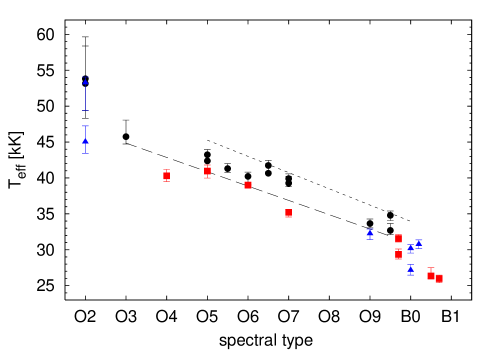
Figure 1: Effective temperatures as a function of spectral type for the investigated LMC sample. Different luminosity classes are denoted using circles, triangles and squares for class V, III and I-II objects, respectively. Shown as a dashed line is the $T_{\rm eff}$ calibration of Martins et al. (2005a) for Galactic O-type dwarfs. The dotted line corresponds to the average effective temperature of the SMC dwarfs studied in Paper II. The LMC dwarfs are found to lie in between these two average scales, with a typical $\sim$2 kK offset from both the average Galactic and SMC relations.

For comparison we also show in Fig. 1 as a dashed line the observed $T_{\rm eff}$ vs. spectral calibration for Galactic O-type dwarfs from Martins et al. (2005a). With a dotted line the average temperature of the SMC dwarfs studied in Paper II is shown. The LMC dwarfs are found to occupy the region in between these two average temperature scales, with an average behaviour intermediate to that of the Galactic and SMC dwarfs. We interpret this as the result of the metallicity of the LMC that is lower than the Galactic value and higher than in the SMC. As the amount of line blanketing in a stellar atmosphere depends on metallicity the LMC objects have temperatures in between that of objects in the other two galaxies.

4.2 The $T_{\rm eff}$ scale of O2 stars

Our sample contains four O2 type stars. This spectral type was introduced by Walborn et al. (2002b) and is assigned based primarily on the ratios of selective emission lines of N iv and N iii. By modelling these lines Walborn et al. (2004) have shown that indeed, as had been hypothesised, the O2 spectra correspond to higher effective temperatures. However, the correct treatment of nitrogen lines in stellar atmosphere models is notoriously difficult. The relevant ionisation stages of this atom represent much more complex ion models compared to the relatively simple hydrogen and helium ions. Moreover, for the higher ions of nitrogen the ionisation depends on the extreme-UV radiation field, which may be affected by non-thermal processes, such as shocks. Adding to the complexity is the fact that the nitrogen abundance has to be treated as a free parameter, as many early type stars show evidence of atmospheric abundance enhancements (e.g. Crowther et al. 2002; Bouret et al. 2003). In our analysis method we solely model the hydrogen and helium lines and self consistently allow for abundance enhancements by treating the helium abundance as a free parameter. In principle our temperature determination should, therefore, not be affected by such problems. As a result of this, our analysis can provide an independent confirmation for the hot nature of O2 stars.

In Fig. 1 we see that the objects with an O2 spectral type indeed correspond to the hottest stars in our sample. With exception of the giant N11-031, which based on its helium lines we find to be cooler (see below), they have temperatures in excess of 50 kK and, therefore, are significantly hotter than the O3 star at $\mbox{$T_{\rm eff}$}=46$ kK. The error bars, though, are considerable. Compared to the average error of $\sim$3 percent the O2 effective temperatures have an uncertainty of 5 up to 11 percent. This large uncertainty can be explained by the weak or even absent neutral helium lines in the spectra of these objects. As a result of this, our fitting method has to predominately rely on the He ii line profiles to determine the correct helium ionisation equilibrium. Based on a single ionisation stage the determination of this equilibrium is more uncertain, which explains the larger error bars. One should also be wary for a possible degeneracy effect between $T_{\rm eff}$ and $Y_{\rm He}$ that can occur as a result of the missing neutral helium lines (see e.g. Paper I, ). This, however, is not an issue as the helium abundances derived for all O2 stars correspond to normal values close to 0.10.

It is also possible to question whether the fact that the He i lines are so weak could result in a systematically higher $T_{\rm eff}$ determination by the automated method compared to “by eye” fits. In other words, would a “by eye” fit prefer a lower temperature solution? For the O2 giant N11-026 this is a relevant question, as the weak He i $\lambda$4471 line, shown in Fig. 14 in the appendix, is not fitted perfectly. Note, however, that due to the relative plot scale the discrepancy is exaggerated and that the fit quality is good and is comparible to that of the He ii lines. Still, to assess whether the fit of this particular line could be improved, i.e. to search for a solution predominantly using the He i diagnostic, we ran test fits with increasing relative weight of He i $\lambda$4471. We found that a solution with an improved fit could be obtained for an increase of the relative line weight with a factor of five. This solution has a $T_{\rm eff}$ lower by 3.7 kK and all other fit parameters approximately equal to the solution with the low He i $\lambda$4471 weight. The overal fit quality of the other lines has somewhat decreased. As these lines are relatively strong, this is difficult to discern by eye. Also note that within the lower error estimate for $T_{\rm eff}$ of 3.9 kK the two solutions agree. Similar results were also obtained for the O2 stars BI 237 and BI 253, where a reduction of $T_{\rm eff}$ by 3.8 kK and 5.4 kK was found, respectively, for an increase in the relative weight of He i $\lambda$4471 by a factor of six and two, respectively. Consequently, based on our analysis we can only give a range for the $T_{\rm eff}$ scale of the O2 stars of $49-54$ kK, the bounds being set by the temperatures based on the He i $\lambda$4471 and hydrogen/He ii diagnostics.

The upper end of our hydrogen/helium based O2 effective temperature range is in good agreement compared to the average effective temperature of 54 kK as determined by Walborn et al. (2004). As we already mentioned the giant N11-031 with a $T_{\rm eff}$ lower by approximately 8 kK compared to the other O2 stars forms an exception to this. Its effective temperature compares better to the temperature of the O3 star N11-060. A close inspection of the spectra of the two stars reveals why this is so. Both stars have exactly the same equivalent width ratio of the He i $\lambda$4471 and He ii $\lambda$4541 lines, which results in similar values for $T_{\rm eff}$. To also test whether the relatively strong He i $\lambda$4471 line could be dominating the fit, forcing a relatively low $T_{\rm eff}$, we refitted the spectrum of N11-031 ignoring the neutral helium lines. This again resulted in an effective temperature of 45 kK.

Interestingly, the nitrogen line analysis of Walborn et al. for N11-031 did result in a higher effective temperature of 55 kK. We are not sure whether this discrepancy is the result of a systematic offset between the N v $\lambda$4603-20/N iv and He i $\lambda$4471/He ii temperature scales. A more recent comparison by one of us (P.A.C.) of the spectral fit of Walborn et al. to new VLT data, however, showed relatively large discrepancies in the helium line fits compared to the nitrogen line fits, indicating that this could be the case. The discrepancy could also be due to differences in fitting assumptions and approaches. Walborn et al. adopted a surface gravity of $\mbox{$\log{{g}}$}=4.0$ and estimated a mass loss rate of $\mbox{$\dot{M}$}=1.0\times 10^{-6}\,\mbox{$M_{\sun}{\rm yr}^{-1}$}$ from the He ii $\lambda$4686 line. Our fit indicates that the former parameter should be lower by 0.15 dex, consequently lowering $T_{\rm eff}$. With respect to the mass loss rate we find a value higher by a factor four. An increase in $\dot{M}$ of this magnitude can have a significant effect on the strength of different nitrogen lines (e.g. Crowther et al. 2002) and, therefore, on the derived effective temperature.

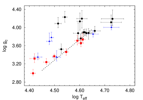
Figure 2: The $\log\mbox{$T_{\rm eff}$}$ – $\log{{g}}_{\rm c}$ plane for the analysed LMC objects. Different luminosity classes are denoted using circles, triangles and squares for dwarfs, giants, and bright giants and supergiants, respectively. With exception of two objects the dwarfs are clearly separated from the luminosity class I-II objects. The giants seem to overlap with both the luminosity class V and I-II objects. Shown as a dotted line is the average $\log\mbox{$T_{\rm eff}$}$ – $\log{{g}}_{\rm c}$ relation of the SMC O-type stars of luminosity class I-II-III from Paper II.

Massey et al. (2005) analysed a total of 11 O2 stars. They could determine the effective temperature for three dwarfs and one giant, with $47.0\,{\rm kK}\lesssim\mbox{$T_{\rm eff}$}\lesssim 54.5\,{\rm kK}$. For the supergiants only lower limits of $\mbox{$T_{\rm eff}$}\gtrsim 42$ kK and higher could be derived. These results are in agreement with our findings. However, these authors note that the correlation with $T_{\rm eff}$ for the O2–3.5 spectral types is not tight. In particular no good agreement was found between the ratios of the N iii and N iv emission lines and the He i and He ii lines. Consequently, a more thorough investigation of the O2 stars based on both the nitrogen and helium spectrum is necessary to resolve this degenerate class adequately.

4.3 Gravities

The distribution of our programme stars in the $\log\mbox{$T_{\rm eff}$}$ – $\log{{g}}_{\rm c}$ plane is presented in Fig. 2. To calculate the surface gravity corrected for centrifugal acceleration ($\log{{g}}_{\rm c}$) the method discussed by Herrero et al. (1992) and Repolust et al. (2004) was adopted. Different luminosity classes are denoted using circles, triangles and squares for, respectively, class V, III and I-II objects. In this figure we see that the dwarfs, with exception of two objects, form a group clearly separated from the latter two groups. In contrast to our findings in Paper II we do not find a clear separation between the dwarfs and giants. Instead the latter group of objects shows an overlap with both luminosity class V and I-II objects.

Shown in Fig. 2 as a dotted line is the average $\log\mbox{$T_{\rm eff}$}$ – $\log{{g}}_{\rm c}$ relation of the SMC O-type stars of luminosity class I-II-III from Paper II. The majority of the evolved LMC objects seem to agree with this trend, that illustrates the evolutionary correlation between effective temperature and surface gravity. However, note that some evolved objects are at considerable distance from the average relation. Thus, a calibration of the two parameters for a given luminosity class should be taken with care (see also Repolust et al. 2004).

The comparison of spectroscopically determined masses ($M_{\rm s}$) with masses obtained from evolutionary calculations is presented in Fig. 3. Using the same symbols as in Fig. 2 dwarfs, giant and supergiants are distinguished. Evolutionary masses ($M_{\rm ev}$) were derived from the evolutionary tracks calculated for a metallicity of $Z=0.4\,\mbox{$Z_{\sun}$}$ from Schaerer et al. (1993). The errors on these masses correspond to the maximum mass interval in the error box spanned by the uncertainties in luminosity and effective temperature.

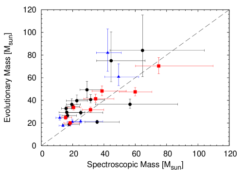
Figure 3: Comparison of spectroscopic masses with masses derived from the evolutionary tracks of Schaerer et al. (1993). The one-to-one correlation between the two mass scales is given by the dashed line. Symbols have the same meaning as in Fig. 2. The objects with the highest evolutionary masses exhibiting a mass discrepancy correspond to the four O2 stars in our sample.

The tracks from Schaerer et al. do not include the effects of rotation. Consequently, this additional source of error is not included. Calculations including $v_{\rm rot}$ show that in some cases one can no longer assign an unambiguous $M(L,\mbox{$T_{\rm eff}$})$. This is a result of rotationally enhanced mixing or the unknown inclination angle, if the star has a non-spherically symmetric distribution of $R_{\star}$ and $T_{\rm eff}$, causing complicated tracks including loops during the secular redward evolution (Meynet & Maeder 2005). Assessing the impact of $v_{\rm rot}$ on the $M_{\rm ev}$ determination we showed in Paper II from a comparison of masses derived from non rotating tracks to those obtained from tracks calculated for $\mbox{$v_{\rm rot}$}=300\,\mbox{km\,s${}^{-1}$}$ that the error in $M_{\rm ev}$ will not increase by more than approximately ten percent.

In Fig. 3 we see that the majority of the objects are located left of the one-to-one correlation, given by the dashed line. The error bars of twelve objects do not even touch this correlation. Consequently, we find a significant mass discrepancy. Similar mass discrepancy problems have been discussed by e.g. Herrero et al. (1992), de Koter & Vink (2003), and Repolust et al. (2004). Most of these classical problems were attributed to limitations in the stellar atmosphere models (Herrero 1993) and to potential biases in the fitting process (see Paper I, ). Here we cannot explain the found discrepancy in such a manner. We will provide a more thorough investigation and discussion in Sect. 5.

4.4 Helium abundances

For the SMC sample that we analysed in Paper II we found a correlation between the helium surface abundance and surface gravity. This could partly be explained by evolutionary effects. As the surface gravity decreases when a star evolves away from the ZAMS, objects with lower gravities would correspond to more evolved objects and are more likely to have atmospheres enriched with helium.

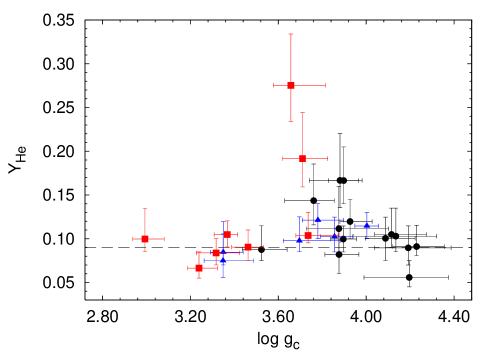
Figure 4: Helium abundances as a function of surface gravity. Symbols have the same meaning as in Fig. 2. The dashed line at $\mbox{$Y_{\rm He}$}=0.09$ is a measure for the initial helium abundance and corresponds to the mean of the helium abundances of the dwarfs with $Y_{\rm He}$ smaller than the sample average. Starting at the highest gravities an increase of the helium fraction is seen down to $\mbox{$\log{{g}}_{\rm c}$}\approx 3.6$.

To investigate whether the scenario discussed above also applies to the current LMC sample, we plot the helium abundance as determined with the automated method as a function of $\log{{g}}_{\rm c}$ in Fig. 4. Also shown as a dashed line is a measure of the initial helium abundance. This value of $\mbox{$Y_{\rm He}$}=0.09$ was calculated by averaging the surface helium abundances of the dwarf type objects with a helium abundance smaller than the total sample average. Compared to this measure for the initial helium abundance a correlation between the surface gravity and helium enrichment can be observed. Starting at the highest gravities, we find an increase in the average helium abundance towards lower $\log{{g}}_{\rm c}$. Note that the two objects exhibiting the largest helium fractions are supergiants. The increase can again be partially explained as an evolutionary effect. In Paper II a similar correlation between average helium abundance and gravity was found to exist down to the lowest gravities investigated.

Interestingly, in Fig. 4 we see that for our LMC sample no helium enrichment is found at $\mbox{$\log{{g}}$}\lesssim 3.6$. Not even the supergiants show evidence of enrichment below this gravity. Why is this so? In Fig. 5, where we present the HR-diagram for our sample, the answer to this question is given. Shown as a grey area in this figure is the region in which the rotating evolutionary models of Meynet & Maeder (2005) predict a helium surface enrichment of at least ten percent. The majority of the evolved objects are located outside this region. Consequently, based on their specific evolutionary phase these objects are not expected to show any enrichment. Also important is the fact that we have selected the hottest objects from the N11 cluster. As a result of this our sample is biased and does not contain the low gravity objects with a high luminosity, i.e. those more likely to be enriched, as these have evolved into cool B-type stars.

Apart from the supergiants also four dwarfs are found to be enriched. Figure 5, in which we have highlighted stars with a helium abundance of at least 0.12 using open symbols, shows that one these dwarfs, Sk $-66$ 18, is located relatively close to the region in which enrichment is predicted. Consequently, rotationally enhanced mixing is a possible explanation. The three remaining dwarfs, N11-60, N11-065 and Sk $-70$ 69, in contrast lie relatively close to the ZAMS. Therefore, “normal” mixing cannot explain their enrichment. Instead, a possible explanation is given by chemically homogeneous evolution. As this may also be linked to the mass discrepancy, we will return to it in Sect. 5.

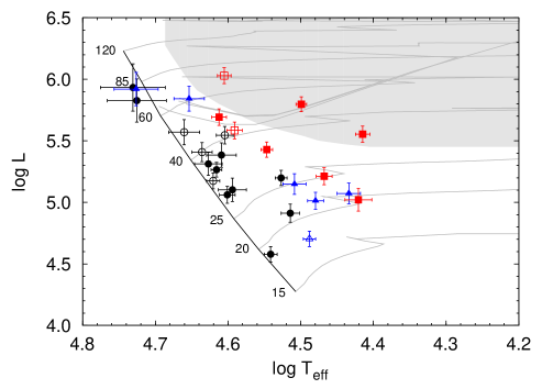
Figure 5: Hertzsprung-Russell diagram for the LMC sample. Symbols have the same meaning as in Fig. 2. Over plotted as grey lines are the evolutionary tracks of Schaerer et al. (1993) for $Z=0.4\,\mbox{$Z_{\sun}$}$, with a black line representing the ZAMS. Open symbols indicate objects with $\mbox{$Y_{\rm He}$}\geq 0.12$. The grey area correspond to the region in which the rotating evolutionary models of Meynet & Maeder (2005) predict a relative helium enhancement of at least 0.01.

4.5 Microturbulence

The microturbulent velocities determined with the automated fitting method are also given in Tab. 2. Though the error estimates are relatively large (see Tab. 3), we find that for the current data set the $v_{\rm turb}$ determinations were sufficiently accurate to reveal a weak correlation between this parameter and the surface gravity. This is shown in Fig. 6, where it can be seen that for $\mbox{$\log{{g}}$}\lesssim 3.6$ the average microturbulence recovered from the line profiles increases systematically. The situation for $\mbox{$\log{{g}}$}\gtrsim 3.6$ is less clear, as the error bars are on average larger and the values for $v_{\rm turb}$ are more or less randomly distributed between 0 and 20 km s^-1. The reason for this is that for larger values of the surface gravity the line profiles become intrinsically broader due to the increased Stark broadening, making it more difficult to accurately recover $v_{\rm turb}$ from the line profiles only.

Based on samples predominantly consisting of unevolved early B-type Galactic stars other authors have also found a relation between microturbulence and surface gravity, e.g. Kilian et al. (1991), Gies & Lambert (1992) and Daflon et al. (2004). More recently Hunter et al. (2006) analysed a sample of early B-type stars in the Magellanic clouds and also found a trend of increasing $v_{\rm turb}$ for decreasing $\log{{g}}$. To derive the values for $v_{\rm turb}$ all these authors relied on curve-of-growth techniques, which were applied to metal lines such as those of Si iii and O iii calculated using plane parallel models. Consequently, our line profile based analysis is an independent confirmation of the existence (or requirement by lack of a physical explanation or failures in the line broadening mechanisms) of microturbulence in the atmospheres of these type of stars.

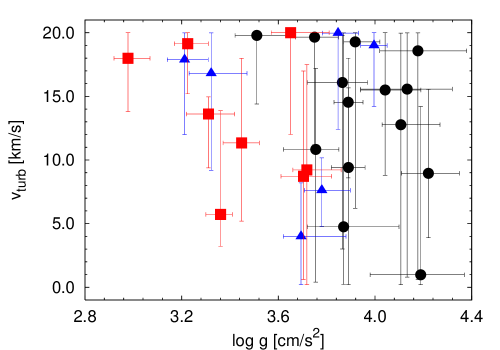
Figure 6: Microturbulent velocities determined using line profile fits as a function of surface gravity. Symbols have the same meaning as in Fig. 2. For $\mbox{$\log{{g}}$}\lesssim 3.6$ a trend of increasing $v_{\rm turb}$ with decreasing $\log{{g}}$ is visible. For larger gravities the uncertainties in the $v_{\rm turb}$ determinations are too large to discern any possible relation.

The physical mechanism explaining the observed microturbulence or its relation to the surface gravity is still poorly understood. Kudritzki (1992) and Lamers & Achmad (1994) have argued that the observed microturbulence might be the result of a stellar outflow, implying the existence of a velocity gradient in the photospheric layers, which can mimic microturbulence-like desaturation effects. Smith & Howarth (1998), however, showed by applying a simple core-halo model to the Galactic O9.7 supergiant HD 152003 that this effect would not be sufficient to explain the observed $v_{\rm turb}$. Indeed, our analysis employing a unified photosphere and wind model confirms that the microturbulence cannot be explained as an artifact of a transonic velocity field.

A possible explanation for the gravity dependence could be related to instabilities in the wind. These instabilities are reflected in the large turbulent velocities ($\sim$100–200 km s^-1) necessary to fit the wind lines in the intermediate and outer wind (e.g. Groenewegen & Lamers 1989; Haser et al. 1998; Evans et al. 2004b) and could be related to shocks due to the intrinsic line-driven instability (Lucy 1983; Owocki et al. 1988; Owocki & Puls 1999). For a low surface gravity the wind starts at larger Rosseland optical depth compared to the high gravity case. Therefore, the line forming region of low gravity objects contains a relatively large contribution originating from (the base of) the wind. Consequently, this region could be affected by the onset of the line-driven instability introducing wind-turbulence into the line profiles.

Figure 7: Microturbulent velocity as a function of the location of the line forming region of He i $\lambda$4471, which is defined as the location where the radial optical depth in the line core reaches a value of $\tau=2/3$. A weak trend is visible that suggests that for increasing extension of the atmosphere larger values of $v_{\rm turb}$ are necessary to fit the line profiles.

Tentative support for the above described scenario may be implied by Fig. 7, where we show $v_{\rm turb}$ as function of the line forming region of He i $\lambda$4471 in units of the stellar radius. The location of the line forming region is defined as the position at which the radial optical depth in the line core reaches a value of 2/3. This figure shows that when the radial distance to this position increases also the average microturbulent velocity increases. Though the trend is weak, it does seem to indicate that when the atmosphere becomes more extended, higher values of $v_{\rm turb}$ are necessary to reproduce the line profiles. It may appear that this implies that the line forming region enters in to the regime where wind turbulence develops. However, for this statement no compelling evidence is available, as we do not find any correlation between $v_{\rm turb}$ and the distance between the line forming region and (for instance) the sonic point. Moreover, for most objects at $R(\tau_{\rm line}=2/3)>1.04$ values of $v_{\rm turb}$ close to the maximum allowed value are found. Consequently, these values should be interpreted as lower limits. Therefore, we can only conclude that our analysis points towards a gradient in the turbulent velocity, possibly connected to a link between microturbulence and wind instabilities, and suggest further investigation in this direction.

4.6 Wind parameters

The wind parameters and their uncertainties determined using the automated method are listed in Tabs. 2 and 3. Compared to our SMC analysis we find that we were able to accurately determine these parameters for a significantly larger number of objects. This is mainly the result of an on average higher signal-to-noise ratio of the spectra as well as of denser winds for the LMC objects compared to their SMC counterparts. In total we determined 22 mass loss rates and 6 upper limits. The upper limits are defined (and can be identified in Tab. 3) by an error bar $-\log\mbox{$\dot{M}$}>1.0$ dex.

To provide a meaningful comparison of the mass loss rates we place the LMC objects in the modified wind momentum luminosity diagram. This diagram shows as function of stellar luminosity the distribution of the so-called modified wind momentum, which is defined as $\mbox{$D_{\rm mom}$}\equiv\mbox{$\dot{M}$}\mbox{$v_{\infty}$}R^{1/2}_{\star}$. Not only does this allow for an assessment of the behaviour of $\dot{M}$ within our sample, it also provides a convenient method to compare the observed wind strengths to the predictions of line driven wind theory. According to this theory $D_{\rm mom}$ is predicted to behave as

$$\log\mbox{$D_{\rm mom}$}=x\log\left(\mbox{$L_{\star}$}/\mbox{$L_{\sun}$}\right)+\log D_{\circ}\leavevmode\nobreak\ ,$$ (1)

where $L_{\star}$ is the stellar luminosity (Kudritzki et al. 1995; Puls et al. 1996). In this equation $x$ is the inverse of the slope of the line-strength distribution function corrected for ionisation effects (Puls et al. 2000). The vertical offset $D_{\circ}$ is a measure for the effective number of lines contributing to the acceleration of the outflow.

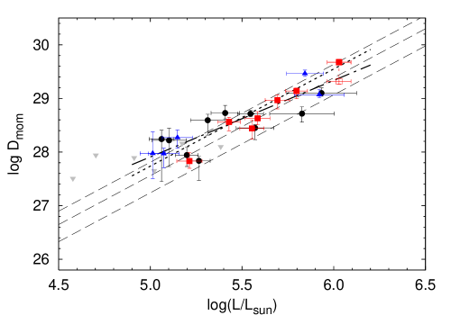
Figure 8: Modified wind momentum ($D_{\rm mom}$) in units of ${\rm g\,cm\,s^{-2}}\,\mbox{$R_{\sun}$}^{1/2}$ vs. luminosity. Symbols have the same meaning as in Fig. 2. Upper limits are shown as inverted triangles. Dashed lines correspond to the predicted wind-momentum luminosity relations (WLR) from Vink et al. (2000, 2001). The upper, middle and lower relation, respectively, correspond to predictions for Galactic, LMC and SMC metallicity. The observed modified wind momenta show a strong correlation with luminosity with an average relation that lies in between the predicted Galactic and SMC WLR. This is quantified by the empirical WLR that was constructed for the LMC objects and that is shown by the dotted line. The open square corresponds to the wind momentum corrected for clumping of the supergiant Sk $-67$ 166. Shown as a dashed-dotted is the empirical WLR obtained using this corrected $D_{\rm mom}$.

In Fig. 8 the distribution of the modified wind-momenta for our programme stars are presented. Indicated using circles, triangles and squares are objects of, respectively, luminosity class V, III and I-II. Upper limits are shown as grey inverted triangles. A clear correlation between $L_{\star}$ and $D_{\rm mom}$ can be observed in this figure. Over an order of magnitude in $L_{\star}$ the average modified wind-momentum decreases by approximately 1.5 dex. A comparison of the behaviour of $D_{\rm mom}$ with predictions is facilitated by the theoretical WLRs calculated by Vink et al. (2000, 2001) that are shown as a set of dashed lines. The upper, middle and lower of these predicted power laws were calculated for, respectively, Solar, LMC and SMC metallicity. Compared to these predictions we find that the LMC wind-momenta are approximately confined between the theoretical WLR for Galactic and SMC metallicity. In other words, compared to the Galactic and SMC case, stars in the LMC have intermediate wind strengths.

To further quantify the behaviour of LMC winds relative to that of Galactic and SMC outflows we have fitted a power law to the observed modified wind-momentum distribution, consistently accounting for both the symmetric errors in $L_{\star}$ and the asymmetric errors in $D_{\rm mom}$, This yielded the following empirical WLR

$$\log\mbox{$D_{\rm mom}$}=(1.81\pm 0.18)\log\left(\mbox{$L_{\star}$}/\mbox{$L_{\sun}$}\right)+(18.67\pm 1.01)\leavevmode\nobreak\ .$$ (2)

The theoretical LMC relation from Vink et al. is given by $x=1.83$ and $\mbox{$D_{\rm mom}$}=18.43$. The error bars of the theoretical and empirical relations are in agreement. More importantly, in Fig. 8 the empirical relation, shown as a dotted line, is found to lie between the predicted Galactic and SMC relations. These predictions have been found to be in good agreement with the observed Galactic WLR (Repolust et al. 2004, Paper I) and observed SMC WLR (Paper II). Consequently, our empirical LMC WLR is quantitative evidence for the fact that massive stars in this system have mass loss rates intermediate between those of massive stars in the Galaxy and SMC.

The differences between the empirical and theoretical LMC WLR at the start and end of the observed luminosity range are, respectively, 0.17 and 0.16 dex. In Fig. 8 this seems to imply a systematic offset between the two relations. However, we note that these differences are still smaller than the typical uncertainty in $D_{\rm mom}$ of 0.2 dex. More importantly, no correction was applied for the possibility that the winds of our sample stars are, in contrast to our assumption, not smooth but structured. In recent years evidence has been mounting for this so-called clumping in the winds of O- and early B-type stars. In particular spectroscopic modelling of UV (resonance) lines (Crowther et al. 2002; Hillier et al. 2003; Bouret et al. 2003; Massa et al. 2003; Martins et al. 2004, 2005b; Bouret et al. 2005; Fullerton et al. 2006) seems to suggest the existence of clumping factors in the range of 10-100, implying corresponding reductions of $\dot{M}$ by factors 3 up to 10. More recently, Puls et al. (2006) also found clumping factors of the order 5 to 10 (normalized to the unknown clumping properties in the outermost, radio-emitting wind) from the analysis of H$\alpha$, infrared, millimetre and radio fluxes. In the present study we try to account for possible wind clumping effects by correcting the mass loss rates of stars with H$\alpha$ in emission. Markova et al. (2004) and Repolust et al. (2004) argue that the mass loss rates of these stars could be overestimated as a result of the fact that H$\alpha$ emission lines are formed over a relatively large volume where clumping might have set in. In contrast, for stars with H$\alpha$ in absorption the line is formed relatively close to the stellar surface, where clumping effects are negligible. Based on the comparison of dwarfs and supergiants in their Galactic sample Repolust et al. derived a numerical correction factor of 0.44 for the mass loss rates of supergiants with H$\alpha$ in emission.

We have applied the clumping correction to the super giant Sk $-67$ 166, which has a H$\alpha$ emission profile. In Fig. 8 its new wind momentum is indicated using an open symbol. Using this value the following empirical WLR is obtained

$$\log\mbox{$D_{\rm mom}$}=(1.43\pm 0.17)\log\left(\mbox{$L_{\star}$}/\mbox{$L_{\sun}$}\right)+(20.77\pm 0.97)\leavevmode\nobreak\ .$$ (3)

In Fig. 8 we see that for $\log\mbox{$L_{\star}$}/\mbox{$L_{\sun}$}\gtrsim 5.3$ the new WLR compares better to the Vink et al. relation. For lower luminosities the situation is less clear. Due to the large uncertainties, this range has a relatively low weight in the fit. Consequently, a discrepancy for low $L_{\star}$ is less significant than the good agreement obtained for the higher luminosities. For this reason it is difficult to investigate the existence of a “weak wind problem” for stars at $\log\mbox{$L_{\star}$}/\mbox{$L_{\sun}$}\lesssim 5.3$, first reported by Bouret et al. (2003). This study, as well as later studies (Hillier et al. 2003; Evans et al. 2004a; Martins et al. 2004, 2005b) report a steepening in the WLR relation relative to predictions starting at about the above mentioned $L_{\star}$, leading to an over prediction of the wind strength by up to a factor 100 at $\log\mbox{$L_{\star}$}/\mbox{$L_{\sun}$}\sim 4.5$. Our LMC results do not appear to confirm this break between observations and seem to follow the predictions down to $\log\mbox{$L_{\star}$}/\mbox{$L_{\sun}$}\approx 5.0$. In a forthcoming paper we will present a comprehensive overview of the observed WLR relations in our Galaxy and the Magellanic Clouds as well as a thorough discussion of the successes and failures of the theory of radiation driven winds in predicting the WLR, including possible causes for the weak wind problem (Mokiem et al. in preparation).

5 The mass discrepancy

In Fig. 9 we investigate the mass discrepancy of our LMC targets as a function of the helium surface abundance. On the vertical axis a measure for this discrepancy is shown, which is scaled to the mean of the evolutionary and spectroscopic mass. This ensures that positive and negative discrepancies follow the same linear scale. For non-enriched stars, i.e. $\mbox{$Y_{\rm He}$}\lesssim 0.10$, approximately three times as many objects lie above the one-to-one correlation than below it. Therefore, in contrast to our finding for the equivalent SMC case (Paper II) a significant mass discrepancy is found for our sample of non-enriched LMC stars. The reason for this is unclear. As we stated before our analysis employs state-of-the-art atmosphere models, and is in principle not hampered, as were previous studies, by potentially unoptimised fits. As stated, in our SMC dataset, analysed in an identical manner, no evidence was found for a mass discrepancy for $\mbox{$Y_{\rm He}$}<0.10$.

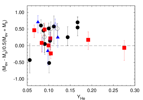
Figure 9: Mass discrepancy as a function of helium abundance for the LMC sample. Evolutionary masses used to calculate the discrepancy were derived from the non-rotating tracks of Schaerer et al. (1993). Symbols have the same meaning as in Fig. 2. The open symbols correspond to stars with $\mbox{$T_{\rm eff}$}\geq 45$ kK.

Massey et al. (2005) also study the $M_{\rm s}$ vs. $M_{\rm ev}$ problem in a set of LMC stars. For objects hotter than 45 kK they find a mass discrepancy that is even stronger than what we find. This behaviour could be the result of an underestimate of the photospheric line pressure in this high temperature regime. In Fig. 9 we have highlighted the objects with $\mbox{$T_{\rm eff}$}\geq 45$ kK using open symbols. Although their mass discrepancy is considerable they do not stand out as a separate group.To further illustrate this, note that the hottest supergiant in our sample Sk $-67$ 166 ($\mbox{$T_{\rm eff}$}=40$ kK) at $\mbox{$Y_{\rm He}$}=0.28$ has a $M_{\rm s}$ of 75 $M_{\sun}$  which is in very good agreement with its $M_{\rm ev}$ of 70 $M_{\sun}$. Consequently, though we can not explain the mass discrepancy we do not anticipate that it is connected to a flawed treatment of the photospheric radiation pressure that manifests itself at metallicities as high as that of the LMC environment (but not yet at values typical for the SMC).

If we accept the analysis of stellar and photospheric parameters, the presence of a mass discrepancy may point to an oversimplified picture of the evolution of massive stars used to determine $M_{\rm ev}$ and/or, possibly, to a breakdown of the assumption of a spherically symmetric atmosphere. One obvious simplification may be that we have used tracks for non-rotating stars. One of the effects introduced by rotation is a wide bifurcation in the evolutionary tracks (Maeder 1987). Stars rotating faster than roughly half the surface break-up velocity will essentially follow tracks representative of homogeneous evolution. Langer (1992) showed that as a result of this the $M/L$-ratio will be a monotonically decreasing function for increasing helium enrichment. Consequently, stars evolving along homogeneous tracks are expected to be increasingly under-massive for increasing helium abundance. One would therefore derive a positive mass discrepancy if the evolution of a rapidly rotating star was incorrectly described using non-rotating or modestly rotating model tracks.

So, can rapid rotation be used to explain the observed mass discrepancy? Let us first focus on the supergiants. For these stars the mass discrepancy problem appears absent, though we note two exceptions at $\mbox{$Y_{\rm He}$}=0.07$ and $\mbox{$Y_{\rm He}$}=0.09$. This absence of signs of a distinct mass discrepancy was also found in our study of SMC bright giants and supergiants (Paper II). The conclusion seems to be that the supergiants follow non-rotating or modestly rotating evolutionary tracks. This implies that, apparently, all supergiant targets that we have selected in both the SMC (Paper II) and LMC happen to have started out their evolution with low or modest initial rotational velocities. As the initial rotational velocity distribution derived in Paper II for the NGC 346 cluster implies that only some $5-15$ percent of stars are expected to evolve along homogeneous tracks this should not be alarming. One supergiant, however, might not fit this picture: Sk -67 166. This source does not feature a mass discrepancy, but does show an increased helium abundance. Given its position in the HRD this is quite difficult to explain in term of evolution without rotation. A scenario accounting for a more delicate interplay between mass loss and rotation may be required to explain its properties (see Herrero & Lennon 2004).

Now let us turn to the dwarfs and giants. For our SMC sample we found a correlation between the helium surface enrichment and the mass discrepancy for class V and III stars, with $M_{\rm s}$ being systematically smaller than $M_{\rm ev}$ for $\mbox{$Y_{\rm He}$}\gtrsim 0.11$. Interestingly, this dependence was only found for dwarfs and giants (see above). It was suggested that this behaviour was the result of rotationally enhanced mixing, enriching the atmospheres with primary helium. The dwarfs and giants at $\mbox{$Y_{\rm He}$}>0.11$ displayed in Fig. 9 also systematically suffer from a positive mass discrepancy. Consequently, this scenario also seems to be a good explanation for the situation in the LMC sample. However, we realise that these seven objects are a relatively small sample and that the typical uncertainties in $Y_{\rm He}$ are 0.03. This statement should therefore be seen as a working hypothesis.

For helium enriched dwarfs and giants the above scenario seems a logical one, as helium enrichment early on in the evolution must imply efficient mixing. For the dwarfs and giants that do not show excess helium in their surface layers such a clue or indication is not present (unless they evolve left of the main sequence as do chemically homogeneous stars, see Sect. 5.1). In principle these non $Y_{\rm He}$-enriched stars could rotate sufficiently rapid to cause a mass discrepancy, but not to the extent of chemically homogeneous evolution. However, if so, a very significant fraction of the stars should have started their evolution at super-critical rotation. At least for the stars studied in the SMC cluster NGC 346 (Paper II) this is not the case.

5.1 Chemically homogeneously evolving O2 stars

Three out of the four O2 stars are found to lie to the left of the ZAMS in Fig. 5 and exhibit relatively large mass discrepancies (see open symbols in Fig. 9). These are N11-026, BI 237 and BI 253. For a discussion of the effective temperature of the fourth O2 object, N11-031 ($\mbox{$T_{\rm eff}$}\sim 45$ kK), we refer to Sect. 4.1. Even though the hottest three ($\mbox{$T_{\rm eff}$}\sim 53-54$  kK) are not significantly enriched in helium it is tempting to speculate on a possible (near) homogeneous evolution of these objects. This would not only provide an explanation for their mass discrepancy, it would also explain their peculiar location in the HRD. The possibility that these are true ZAMS stars is very exciting. However, due to the short evolutionary time scales in this part of the HR-diagram, it would also be unlikely. Based on the non-rotating model tracks of Schaerer et al. (1993) we estimate that a 60 $M_{\sun}$ star will within 2 Myr evolve away from the ZAMS to a location in the HRD at $\mbox{$T_{\rm eff}$}\approx 45$ kK. This is well beyond the error bars on the parameters of these objects. Given the fact that N11-026 and BI 253 are thought to be associated with the LH 10 and 30 Doradus clusters, respectively, which have ages of approximately 3 (see Sect. 6.2) and 2 Myr (de Koter et al. 1998), a normal evolutionary scenario appears unlikely. Based on its large radial velocity the field star BI 237 probably is a runaway star (Massey et al. 2005), therefore it is also likely to be relatively old.

The problems with a reconciliation of the hottest three O2 stars with fully homogeneous evolution and an age of at least 2 Myr, are i) that their surface helium abundances are not significantly enriched, and ii) that their rotational velocities are not extreme. The latter issue need not be “a smoking gun” considering the possibility that we may see them relatively pole-on and the fact that their $v_{\rm r}\sin i$ values, ranging between 110-190 km s^-1, are above the sample average. Concerning the first point, it appears that we must concede to the possibility that stars may evolve along tracks similar to those for homogeneous evolution while in fact they are not fully homogeneous – i.e. the near surface layers are not yet strongly affected by the mixing that must occur deeper in. Having said this, we do point to the fact that the error bars on $Y_{\rm He}$ do allow for relatively large ages even within the hypothesis of fully homogeneous evolution. Within the error bars the maximum $Y_{\rm He}$ is $\sim$ 0.13 for all three stars. It takes fully homogeneously evolving stars of 60 and 40 $M_{\sun}$ about $\sim 1.5$ and $\sim$2.0 Myr, respectively, to build up this amount of helium enrichment (S. -C. Yoon, private communication). This is close to the derived cluster ages of LH 10 and 30 Doradus. For reference, if the star would evolve along near-homogeneous tracks they would be older.

We tentatively conclude that the HRD position, helium abundance, and rotational velocity of the three hottest O2 stars in our sample could be consistent with (near-)homogeneous evolution. Evidence for efficient rotation-induced mixing during the main sequence phase of O stars has also been presented by Lamers et al. (2001), based on the chemical abundance pattern of ejected circumstellar nebulae.

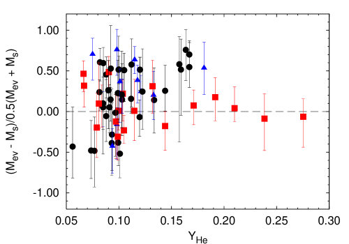
Figure 10: Mass discrepancy as a function of helium abundance for the combined samples from Paper I (Galactic), Paper II (SMC) and the current LMC sample. Symbols have the same meaning as in Fig. 2. Note the good correspondence between $M_{\rm s}$ and $M_{\rm ev}$ for the bright giants and supergiants (square symbols).

5.2 Large sample trends

To firmly establish our findings with respect to the mass discrepancy problems, we compare in Fig. 10 spectroscopic and evolutionary masses for all stars that have been analysed using our automated fitting method so far. Presented in this figure are the combined Galactic (Paper I), SMC (Paper II) and the current LMC samples, corresponding to a total of 71 O- and early B-type stars.

Figure 11: The FLAMES field for the star forming region N11 with the associations LH9 (south of centre) and LH10 (north of centre). The FLAMES targets are identified using circles and their star identification is given. From Evans et al. (2006). [Included as separate JPG file in astro-ph submission.]

The figure confirms our two main findings. First, the good agreement between $M_{\rm s}$ and $M_{\rm ev}$ for the supergiants is clearly visible. This is an encouraging finding and we believe that this means that the improvements in the stellar atmosphere models, evolutionary calculations and spectral analysis techniques have finally resolved the long standing mass discrepancy as found by Herrero et al. (1992). The correspondence between the spectroscopic and evolutionary mass scale, in particular for increasing helium enrichment is striking. The reason for this is probably related to the fact that the class I-II objects are found in the region of the HR-diagram in which stars are not expected to undergo extreme evolutionary phases, such as homogeneous evolution. Consequently, the enriched bright giants and supergiants have evolved along relatively simple evolutionary tracks, which (in this respect) appear well understood.

Our second finding, i.e. that of a correlation of mass discrepancy with the helium abundance, is also corroborated by the large sample in Fig. 10. For $\mbox{$Y_{\rm He}$}>0.10$ all dwarfs and giants, except for one dwarf, are found above the $\mbox{$M_{\rm s}$}=\mbox{$M_{\rm ev}$}$ line. In all fairness, given the typical uncertainty of 0.03 in $Y_{\rm He}$, from a statistical point of view the region $0.09<\mbox{$Y_{\rm He}$}<0.12$ should be regarded with care. For larger helium abundance, however, the correlation can be regarded to be statistically significant. A total of 11 objects show a positive mass discrepancy, with only a single counter example. Moreover, the magnitude of the discrepancy seems to be related to the amount of enrichment. This strongly points to efficient mixing in the main sequence phase, leading to (near-)chemically homogeneous evolution.

6 The evolutionary status of N11

In this section we explore the evolutionary status of the N11 field. We will first briefly outline the current understanding of N11 with respect to the OB associations LH9 and LH10 and in particular the sequential evolutionary link between the two. Based on the analysis of the 22 stars in our sample associated with these clusters we will then estimate their ages and discuss whether they are compatible with a sequential star formation scenario.

6.1 LH9 and LH10 in N11

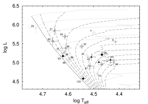
Figure 12: Comparison of the programme stars located in N11 with isochrones derived from the evolutionary tracks of Schaerer et al. (1993). The symbols used to denote dwarf, giants and bright- and supergiants are, respectively, circles, triangles and squares. Filled and open symbols are used to distinguish stars associated with LH9 and LH10, respectively. Black symbols refer to objects located within a radius of two arc minutes of the LH9 and LH10 core, whereas the grey symbols correspond to stars found outside this radius. Labels correspond to the N11 identification numbers given in Tab. 1. Isochrones (dashed lines) are shown from one up to ten million years with 1 Myr intervals. For reference evolutionary tracks from Schaerer et al. (1993) are drawn as grey lines, where for clarity purpose only the blueward part of the evolution for the most massive tracks is shown. The ZAMS corresponding to these tracks is given by the black solid line.

N11 is an intricate giant H ii region containing several massive star forming complexes. The largest of these are the OB associations LH9 and LH10 (Lucke & Hodge 1970). An image of the region, including the adopted star identifications, is presented in Fig. 11 (Evans et al. 2006). Several studies have suggested that the star forming activity in these associations are linked. In particular the study by Parker et al. (1992) has provided a key to understanding of the structure and formation of LH9 and LH10. Their analysis of the stellar content of N11 revealed the presence of several O3-O5 stars and possible ZAMS stars in LH10. In contrast the earliest spectral type associated with LH9 was found to be O6. They also found the slope of the initial mass function of LH10 to be significantly flatter than that of LH9, indicating that the former contains a higher ratio of high mass to low mass stars. Combined with the fact that the reddening of LH10 is larger than that of LH9, it was concluded that LH10 is the younger of the two clusters. Based on these findings the authors propose an evolutionary link between the two, where star formation in LH10 could possibly be triggered by the stellar winds and supernovae of massive stars in LH9.

Further evidence for a sequential star formation scenario was given by Walborn & Parker (1992), who found a dual structural morphology of N11 analogous to that of the 30 Doradus H ii region. In the latter substantial evidence suggests the presence of current star formation in regions surrounding the central star cluster (e.g. Walborn & Blades 1987; Hyland et al. 1992, also see Walborn & Blades 1997). This secondary burst seems to be set off approximately 2 Myr after the initial star formation took place, possibly initiated by the energetic activity of the evolving cluster core. Walborn & Parker argue that this is very similar to N11 where the stellar content of LH9 and LH10 also suggests an age difference of $\sim$2 Myr (also see Walborn et al. 1999). The process in N11, however, would be advanced by $\sim$2 Myr, classifying it as an evolved 30 Doradus analogue, though less massive.

More recently, several bright IR sources showing characteristics of young stellar objects were discovered in the N11B nebula surrounding LH10 by Barbá et al. (2003). These objects are probably intermediate mass (pre-)main-sequence Herbig Ae/Be stars belonging to the same generation as do the LH10 objects (the pre-main-sequence evolutionary timescales of intermediate mass stars being longer than that of massive OB stars). Barbá et al. also found that the massive stars in LH10 have blown away their ambient molecular material and are currently disrupting the surface of the parental molecular cloud material surrounding LH10 (i.e. the material in N11B).

6.2 The ages of LH9 and LH10

To estimate the ages of our programme stars we compare their location in the HR-diagram to theoretical isochrones in Fig. 12. The luminosity classes V, III and I-II are represented using, respectively, circles, triangles and squares. To differentiate between stars associated with LH9 and LH10, respectively, filled and open symbols are used. Membership is defined on the basis of minimum distance to either the LH9 or LH10 cluster core. This, therefore, should be taken with some care: the cores are about 4 arcmin or 60 parsec apart, which can be traversed in 2 Myr if the proper motion of the star is some 30 km s^-1. Runaway O- and B-type stars have typical velocities of 50–100 km s^-1, therefore, it is entirely possibly that (a few) individual objects are assigned to the wrong association. For position reference see Fig. 11. Isochrones in Fig. 12 are shown as dashed lines for one up to ten million years with 1 Myr intervals and were derived from the evolutionary tracks of Schaerer et al. (1993). Note that these tracks do not account for the effects of rotation.

The distribution of the stars in Fig. 12 is such that they can be separated in a group of objects younger than three million years and a group of objects older than this age. We also see that the oldest objects are predominantly found in LH9, whereas LH10 contains the largest fraction of young objects, suggesting that the clusters can indeed be separated in terms of age. At first sight it seems that they can be characterised by an age of $\sim$7 Myr and $\sim$2 Myr, respectively. However, a significant number of objects in both clusters are found to be several million years younger and older than these preliminary ages. A possible explanation for this large age scatter could be “contamination” by field stars. To assess this possibility we have assigned grey symbols to all objects outside a radius of two arc minutes from the cluster cores. Disregarding these objects reduces the age scatter significantly; still a number of stars appear to contradict with the notion of two coeval populations.

To investigate the age distributions in more detail the individual age estimates are shown in Fig. 13. LH9 and LH10 objects, which are shown using the identical symbols as in Fig. 12, are placed in, respectively, the left and right part of the diagram and are separated using a dashed line. First concentrating on the LH9 objects we see that they are near-coeval with exception of four dwarfs. Of these the two non-core members are located at a distance of approximately six arc minutes from the central concentration. Therefore, it is probable that they are either spatially not related to N11 or that possibly their formation was triggered more recently by the stellar activity in LH9. The third dwarf N11-065 occupies a location very close to the ZAMS and in principle would be the youngest member of LH9. However, we also find a considerable helium enrichment for this object ($Y_{\rm He}$= 0.17). Combined with the fact that N11-065 has a large mass discrepancy, this suggests that it might be evolving chemically homogeneously. Consequently, a more appropriate age estimate should be derived from tracks appropriate for this kind of evolution. Adopting such tracks from Yoon et al. (2006, also see ) we derive a lower limit of 6 Myr for the age of N11-065 based on the surface helium abundance. In Fig. 13 this estimate is indicated using an upward pointing arrow, and is in good agreement with the bulk of the LH9 stars.

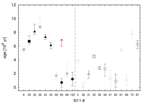
Figure 13: Individual age estimates for stars in N11 based on the non-rotating tracks of Schaerer et al. (1993). Symbols have the same meaning as in Fig. 12. The left and right part of the diagram, respectively, contain stars associated with LH9 and LH10 and are separated using a dashed line. The upward pointing arrow denotes a lower age limit for N11-065 determined from its surface helium abundance using chemically homogeneous evolutionary models (Yoon et al. 2006; Yoon & Langer 2005).

The dwarf N11-123 exhibits no chemical peculiarities and its location on the sky places it in the central concentration of LH9, suggesting that it should have been formed in the burst of star formation that formed the cluster. However, given the fact that N11-123 is in principle the only star deviating from the coeval nature of LH9 we suspect that it is like N11-058 and N11-066 part of the periphery of the cluster and that its relatively close position to the core is due to a projection effect. Consequently, we conclude that the central concentration of LH9 is coeval with an age of $\sim$7.0 $\pm 1.0$ Myr. The error bar is of the same order of magnitude as the 0.5–1.0 Myr introduced by uncertainties in the evolutionary tracks due to effects of (relatively modest) rotation (see Paper II, ).

The right part of Fig. 13 shows that the stars in the central concentration of LH10 have ages ranging from one up to approximately six million years. Despite this large scatter it is clear that the majority of the stars are younger than 4.5 Myr and that only one object (N11-087) in the cluster core is older than this age. An explanation for the large age of the latter object might be that it formed in LH9 and, over time, migrated towards LH10. As explained at the start of this section, this is a possibility given that the distance from the centre of LH9 to the current position of N11-087 is only three arc minutes. Considering the error bars on the age determinations and the additional uncertainty of 0.5–1.0 Myr introduced by rotation (see Paper II, ), we finally estimate an age best describing LH10 of $\sim$3.0 $\pm 1.0$ Myr.

6.3 Sequential star formation?

If the starbursts in N11 are sequential the formation of LH10 should be induced by supernova explosions and/or stellar winds in LH9. Given the age difference and distance between the two clusters we find that both means of triggering are possible. In the first case the age difference of approximately four million years is compatible with the time of $\sim$3 Myr it takes before the most massive stars end their life in a supernova (e.g. Schaller et al. 1992). The time needed for the supernova shock to cross the distance of $\sim$3 arc minutes between LH9 and LH10, corresponding to approximately 40 parsec at the distance of the LMC, is only $\sim$$10^{5}$ years (see e.g. Falle 1981); hence it is a possible scenario. If we consider triggering through stellar winds, the time scales are also compatible. Garcia-Segura et al. (1996), for instance, using hydrodynamical simulations have shown that a 60 $M_{\sun}$ star can create a wind-driven bubble in the interstellar medium of $\sim$50 pc during its main sequence lifetime of 3 Myr. Consequently, this scenario seems to be appropriate as well and in agreement with the determined time scales.

In view of the above we conclude that a sequential scenario for LH9 and LH10 seems very likely. A combination of supernovae and stellar winds from stars in LH9 may have initiated star formation in LH10.

7 Summary and conclusions

We have analysed a sample of 28 massive OB-type stars located in the LMC. For a homogeneous and consistent treatment of the data we employed the automated fitting method developed by Mokiem et al. (2006), which combines the genetic algorithm based optimisation routine pikaia (Charbonneau 1995) with the fast non-LTE unified stellar atmosphere code fastwind (Puls et al. 2005). The sample is mostly drawn from the targets observed within the context of the VLT-FLAMES survey of massive stars (Evans et al. 2005). In total 22 of these stars are located in the LH9 and LH10 clusters within the giant H ii region N11. This region is believed to have been the scene of sequential star formation, with the stellar activity in LH9 igniting secondary starbursts in different associations in N11. Our main findings are summarised below.

1. The effective temperature per spectral sub-type of the LMC stars is found to be intermediate between that of Galactic and SMC O- and early B-type stars, with the LMC objects being, respectively, cooler and hotter by typically $\sim$2 kK.

2. Based on the helium and hydrogen lines it was possible to determine the effective temperatures, though with relatively large error bars, of the four O2 stars in our sample. Three of these are found to be hotter by more than 3 to 7 kK (see Sect. 4.2) compared to the O3 star in our sample, suggesting that O2 stars indeed represent a hotter subgroup within the O-type class. However, we note that for the one ON2 star a relatively low $T_{\rm eff}$ of 45 kK was obtained, indicating that the N iv and N iii classification lines (Walborn et al. 2002b) are not fully compatible with the helium lines traditionally used for classification.

3. The spectroscopically determined masses of the dwarf and giant stars in our set of programme stars are found to be systematically smaller than those derived from non-rotating evolutionary tracks. For helium enriched dwarfs and giants, i.e. those having $\mbox{$Y_{\rm He}$}>0.11$, we find that all show this mass discrepancy. The same was found in an analysis of SMC stars using the same methods (Mokiem et al. 2006). We interpret this as evidence for efficient rotationally enhanced mixing leading to the surfacing of primary helium and to an increase of the stellar luminosity.

4. The bright giants and supergiants do not show any mass discrepancy, regardless of the surface helium abundance. This also is consistent with the finding for Galactic and SMC class I-II objects studied with the same methodology (Mokiem et al. 2005, 2006). This suggests that shortly after birth all these stars must have rotated at less than about 30 to 40 percent of the surface break-up velocity.

5. A weak correlation is found between microturbulent velocity and surface gravity. More extended atmospheres (i.e. lower gravity stars) require a relatively large $v_{\rm turb}$ to fit the lines. The reason for this relation is unclear, however, it does not seem to be connected to the lines being formed closer to the sonic point of the wind flow in low gravity stars.

6. From a comparison of modified wind momenta $D_{\rm mom}$ we find that the wind strengths of LMC stars are weaker compared to Galactic stars, and stronger compared to SMC stars. Comparing the derived $D_{\rm mom}$ as a function of luminosity with predictions for LMC metallicities by Vink et al. (2001) yields good agreement in the entire luminosity range that was investigated ($5.0<L/\mbox{$L_{\sun}$}<6.1$).

7. We have determined an age of, respectively, $\sim$7.0$\pm 1.0$ Myr and $\sim$3.0$\pm 1.0$ Myr for the clusters LH9 and LH10. The age difference and relative distances are in good agreement with a sequential star formation scenario, in which stellar activity in LH9 triggered the formation of LH10.

Appendix A Fits and comments on individual objects

The observed spectra shown in this section were corrected for radial velocities. If not noted differently the lines that were fitted are the hydrogen Balmer lines H$\alpha$, H$\gamma$ and H$\delta$; the He i singlet line at 4387 Å; the He i triplet lines at 4026, 4471 and 4713 Å; and the He ii lines at 4200, 4541 and 4686 Å. Over plotted are the best fit spectra, unless noted differently. For a discussion of the line weighting scheme adopted in our fitting procedure we refer to Paper I (especially to their Table 3.).

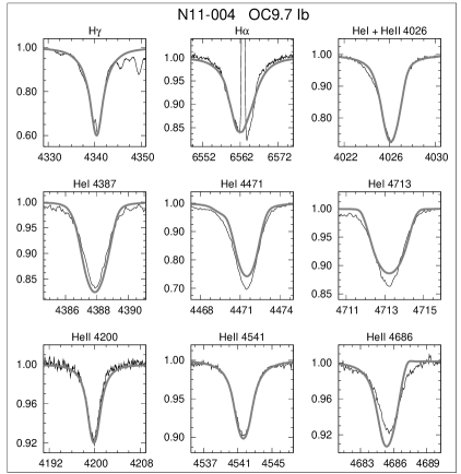
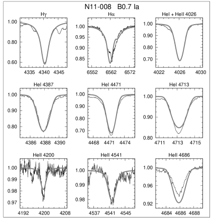
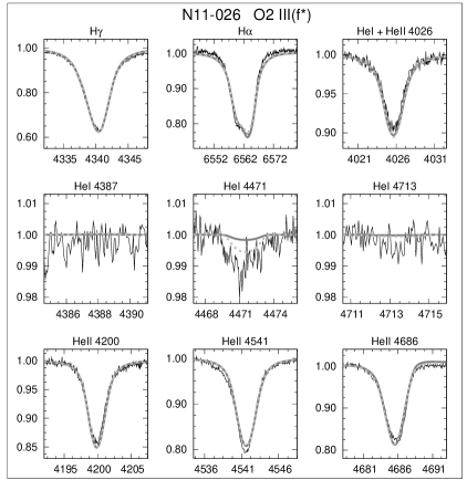
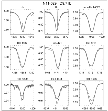
Figure 14: Comparison of the observed line profiles of N11-004, -008, -026 and -028 with best fitting synthetic line profiles obtained using the automated fitting method (grey lines). Wavelengths are given on the horizontal axis in Å. The vertical axis gives the normalised flux. Note that this axis is scaled differently for each line. The dotted line profiles for N11-026 correspond to the best fit obtained adopting a five times larger relative weight for the He i $\lambda$4471 line. This best fit has a $T_{\rm eff}$ lower by 3.7 kK and all other fit parameters approximately equal compared to the fit for the nominal He i $\lambda$4471 weight.

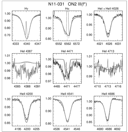
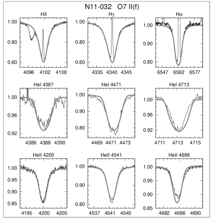
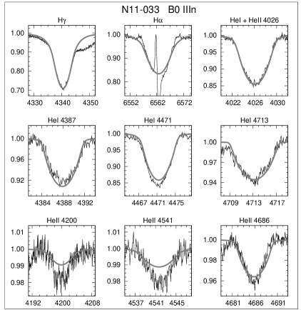
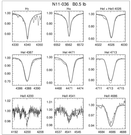
Figure 15: Same as Fig. 14, however, for N11-031, -032, -033 and -036. Shown as dotted profiles for N11-031 is the effect of and a 2.2 kK increase in $T_{\rm eff}$.

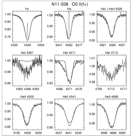
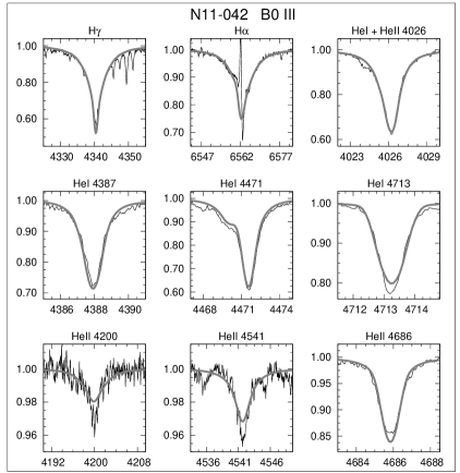
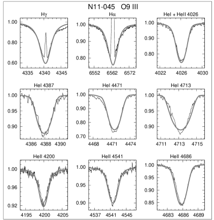
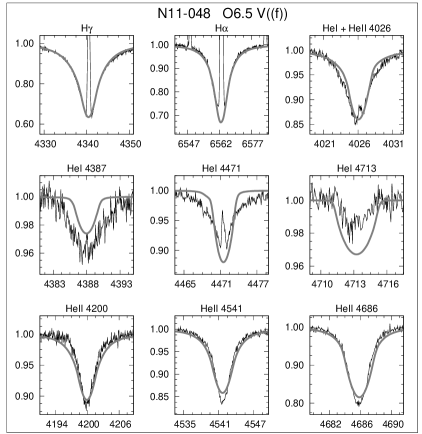
Figure 16: Same as Fig. 14, however, for N11-038, -042, -045 and -048.

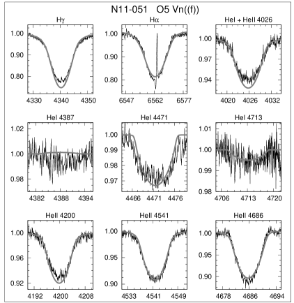
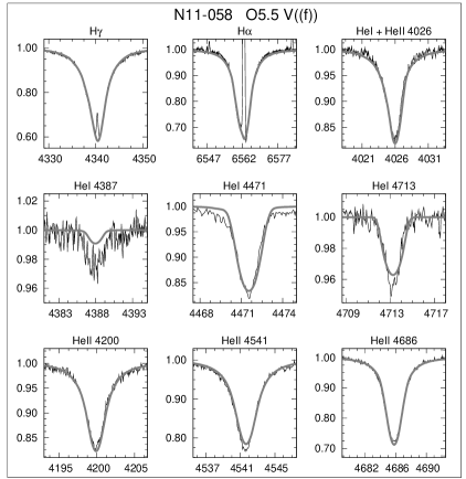
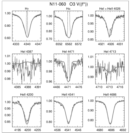
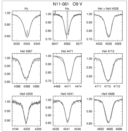
Figure 17: Same as Fig. 14, however, for N11-051, -058, -060 and -061.

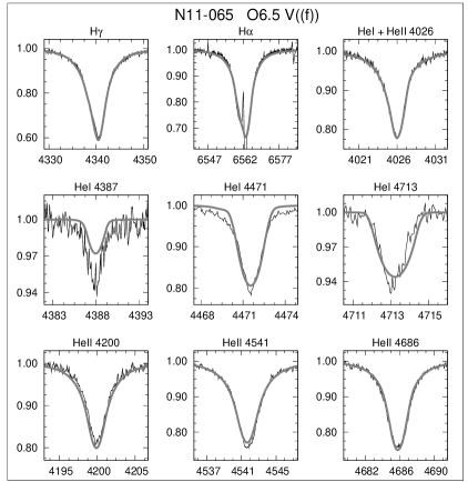
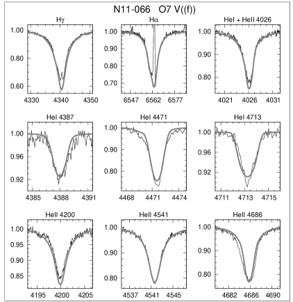
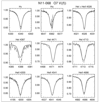
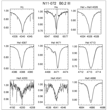
Figure 18: Same as Fig. 14, however, for N11-065, -066, -068 and -072.

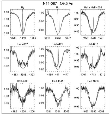
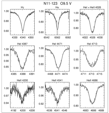
Figure 19: Same as Fig. 14, however, for N11-087 and -123.

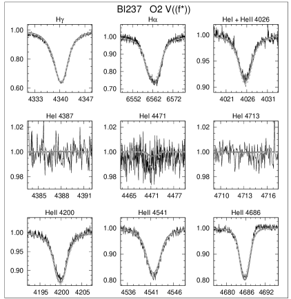
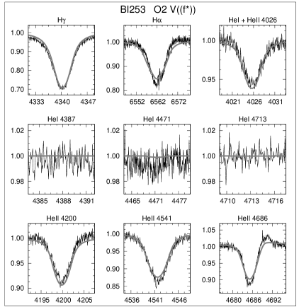
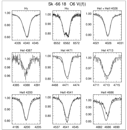
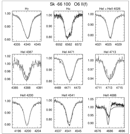
Figure 20: Same as Fig. 14, however, for BI 237, BI 253, Sk $-66$ 18 and Sk $-66$ 100. The dotted profiles for BI 237 correspond to a model calculated with a $T_{\rm eff}$ reduced by 3.8 kK compared to the best fit value. For Sk $-66$ 100 the dotted profiles show the effect of an increase in $\dot{M}$ by 0.12.

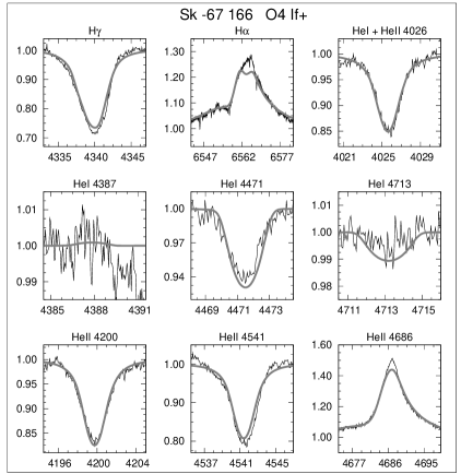
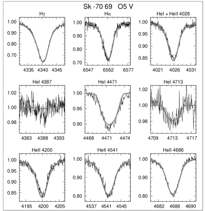
Figure 21: Same as Fig. 14, however, for Sk $-67$ 166 and Sk $-70$ 69.

N11-004

(Fig. 14) With exception of He i $\lambda$4471 good fits for all lines of this OC9.7 supergiant were obtained. The under prediction of the He i $\lambda$4471 line is possibly connected to the so-called generalised dilution effect (Voels et al. 1989, see also Repolust et al. 2004).

N11-008

(Fig. 14) All lines are reproduced well. Note that given the weakness of He ii $\lambda$4686 and lower weight assigned to this line, the reproduction of its profile can be considered good.

N11-026

(Fig. 14) A high effective temperature of 53 kK was needed to fit the spectrum of this O2 giant. Note that even though on its relative plot scale the very weak He i $\lambda$4471 line is not fitted perfectly, the quantitative fit quality is good and is comparible to that of the He ii lines. Still, trying to assess whether the fit could be improved we ran test fits with increasing relative weight of the He i $\lambda$4471 line. It turned out that an increase of a factor of five was necessary to obtain a solution with an improved He i $\lambda$4471 line fit, which is shown in Fig. 14 as a set of dotted lines. This best fit has a $T_{\rm eff}$ lower by 3.7 kK and all other fit parameters approximately equal compared to the regular fit. The overal fit quality of the other diagnostic lines is somewhat less, though this is difficult to discern by eye because these lines are relatively strong (one has to zoom in to the 0.5 to 1 percent level, as we do for He i $\lambda$4471). Note, however, that the error estimates for $T_{\rm eff}$ are relative large and within the lower error estimate of 3.9 kK (cf. Tab. 3) the solutions agree. Also note that even for the lower $T_{\rm eff}$ solution this O2 star is still considerably hotter than an O3 star (see Sect. 4.1).

N11-029

(Fig. 14) A good fit was obtained. The slight underestimation of the core strength of the He ii $\lambda$4200 and He ii $\lambda$4541 lines is, given the relative weakness of these lines, not significant.

N11-031

(Fig. 15) To fit the spectrum of this O2 star a relatively low effective temperature of 45 kK was necessary. Walborn et al. (2004) derived a $T_{\rm eff}$ of 55 kK for this object. However, their determination of this parameter was based on the analysis of the N iv-v ionisation adopting a fixed gravity of $\mbox{$\log{{g}}$}=4.0$. Based on the analysis of the helium ionisation we exclude a $T_{\rm eff}$ higher than $\sim$47 kK. This is illustrated by the dotted lines, which correspond to a model calculated for an effective temperature higher by the upper error estimate we derived for $T_{\rm eff}$. For even higher temperatures the He i $\lambda$4471 would, in contradiction to the observations, disappear completely (also see Sect. 4.1).

N11-032

(Fig. 15) The He i and He ii blend at 4026 Å was not observed for this object. In the final fit, therefore, also the H$\delta$ Balmer line is shown.

N11-033

(Fig. 15) This B0 giant is fast rotator. To reproduce the observed line profiles a projected rotational velocity of 256 km s^-1 was necessary. In the presented fit the strength of He ii $\lambda$4541 seems to be under predicted. However, given the relative weakness of this line this small discrepancy is negligible. Note that the sharp change in the central part of the H$\alpha$ profile is the result of an over subtraction of the core nebular feature and was not taken into account in the fitting procedure.

N11-036

(Fig. 15) The line profiles of N11-036 could be reproduced quite accurately because of its relatively slow rotation.

N11-038

(Fig. 16) The relatively poor reproduction of He i $\lambda$4387 in this O5 bright giant is the result of the low weight assigned to this line based on the spectral type of N11-038. A good fit to the He i $\lambda$4471 could not be obtained due to its peculiar line profile shape. Possibly this triangular profile is related to macroturbulence.

N11-042

(Fig. 16) A relatively low projected rotational velocity was found for this B0 giant allowing for a nearly perfect fit.

N11-045

(Fig. 16) A good fit was obtained for this O9 giant. Despite the good fit quality a problem is apparent when $M_{\rm s}$ and $M_{\rm ev}$ are compared in Tab. 2. The spectroscopic mass is found to be less than half its evolutionary equivalent.

N11-048

(Fig. 16) Based on the fact that the He ii $\lambda$4686 is the strongest line in its spectrum Parker et al. (1992) classified this star as a Vz star. The fit parameters, however, place this object at a considerable distance from the theoretical ZAMS in Fig. 5. We also find that the spectrum can not be reproduced accurately. The width of the neutral helium lines is systematically unpredicted, whereas the width of the He ii is over predicted. This and the fact that the helium abundance that is recovered from the spectrum is rather low ($\mbox{$Y_{\rm He}$}=0.06$) are indicative of a possible binary nature.

N11-051

(Fig. 17) The spectrum of the O5 dwarf N11-051 shows very broad lines, indicating fast stellar rotation. To obtain the final fit a projected rotational velocity of 333 km s^-1 was required.

N11-058

(Fig. 17) A good fit was obtained for all lines of this O5.5 dwarf. The small under prediction of the He i4387 line strength is the result of the relatively low weight assigned to this line for the spectral type of this star.

N11-060

(Fig. 17) Note that the He i $\lambda$4471 line of this O3 dwarf has a strength that is comparable to the strength of this line in the spectrum of the O2 giant N11-031. As the effective temperature we find for these two objects are also comparable, the helium spectrum suggest a spectral type of O3 for both objects.

N11-061

(Fig. 17) All lines of this O9 dwarf are reproduced correctly. The mass loss could be reliably determined using the automated method at a rate of $2.1\times 10^{-7}\,\mbox{$M_{\sun}$}$. Note that the value of 1.8 obtained for the wind acceleration parameter $\beta$ is rather high for a dwarf type object.

N11-065

(Fig. 18) A relatively high helium abundance of 0.17 was recovered from the spectrum. The good fit quality obtained for all lines, however, does not indicate an overestimation of this parameter. A strong mass discrepancy is found with $M_{\rm s}$ being smaller than $M_{\rm ev}$ by approximately a factor of two.

N11-066

(Fig. 18) Apart from a slight under prediction of the width of He ii $\lambda$4686 all lines of this O7 dwarf could be fitted with good accuracy. Like the previously discussed object, again a large mass discrepancy is found with a ratio of $M_{\rm ev}$ to $M_{\rm s}$ of 1.8.

N11-068

(Fig. 18) The final fit reproduces the observed line profiles very accurately. No further comments are required.

N11-072

(Fig. 18) The star has a very sharp lined spectrum. The best fit required a $v_{\rm r}\sin i$ of 14 km s^-1. Note that given the lower error estimate, given in Tab. 3, and the spectral resolution of the data this value can also be interpreted as an upper limit.

N11-087

(Fig. 19) To fit the spectrum of N11-087 a $v_{\rm r}\sin i$ of 276 km s^-1 was needed. The final fit shows a good reproduction of the line profiles with a slight under prediction of the He ii $\lambda$4541 line. Given the signal-to-noise ratio of the spectrum and the relative strength of this line, we do not believe this to be significant.

N11-123

(Fig. 19) Like the previously discussed object N11-123 is also classified as an O9.5 dwarf. The effective temperature needed to fit the spectrum is, however, higher by more than 2 kK. This is the result of a $\log{{g}}$ that is higher by $\sim$0.2 dex.

BI 237

(Fig. 20) A good fit was obtained for this O2 dwarf star. The He i $\lambda$4471 line is hardly visible. Fortunately, the hydrogen and He ii lines provide the automated fitting method with enough information to determine an effective temperature. The error estimates on this parameter, however, are considerable (see Tab. 3). The effect of lowering $T_{\rm eff}$ to the lower error estimate of 49 kK is illustrated by the dotted profiles.

BI 237 was recently also analysed by Massey et al. (2005). Compared to this study we find large differences for $T_{\rm eff}$ ($+5$ kK), $\log{{g}}$ ($+0.2$ dex) and $\dot{M}$ ($-0.4$ dex). Our solution for higher effective temperature and surface gravity can be explained by the fact that the ionisation structure of the atmosphere is set by both these parameters (also see Paper I). The reduced mass loss rate we find is the result of the increased value for $\beta$ ($+0.4$) obtained by the automated method.

BI 253

(Fig. 20) The star has as an identical spectral type as the previously discussed object. The photospheric parameters determined from the spectrum are also very similar to the parameters of BI 237. Note that in contrast to this agreement BI 253 is found to have a much denser wind. Its mass loss rate is larger by a factor 2.5 and reflects the fact that compared to BI 237 the wind lines H$\alpha$ and He ii $\lambda$4686 are more filled in. In their analysis Massey et al. (2005) could only determine a lower estimate for $T_{\rm eff}$ of 48 kK, which is consistent with our lower error estimate. The other parameters determined by these authors are in fair agreement with our analysis. An exception to this is the surface gravity for which Massey et al. estimate a value lower by 0.3 dex, which is the result of the lower $T_{\rm eff}$ used for their fit.

Sk $-$66 18

(Fig. 20) With exception of the He ii lines at 4541 Å and 4686 Å we obtained a near perfect fit. The helium abundance $\mbox{$Y_{\rm He}$}=0.14$ indicates an enriched atmosphere.

Sk $-$66 100

(Fig. 20) was previously analysed by Puls et al. (1996). Compared to this study we find similar parameters with exception of a lower $T_{\rm eff}$ which is the result of the inclusion of blanketing and an increased helium abundance of $\mbox{$Y_{\rm He}$}=0.19$. The final fit shows that with this large value all lines could be reproduced quite accurately. The slight mismatch of the He ii $\lambda$4686 line can be improved by increasing $\dot{M}$ to its upper error estimate. The effect of this increase of 0.12 dex on the line profiles is shown using dotted lines.

Sk $-$67 166

(Fig. 21) This supergiant has both H$\alpha$ and He ii $\lambda$4686 in emission indicating the presence of a dense stellar outflow. To correctly reproduce the line profiles a very high mass loss rate of $9.3\times 10^{-6}\,\mbox{$M_{\sun}{\rm yr}^{-1}$}$ was required. This value is in good agreement with the findings of Crowther et al. (2002) who studied this objects using the model atmosphere code cmfgen (Hillier & Miller 1998) in the optical, UV and far-UV. Compared to these authors we also find that the other fit parameters are in good agreement. An exception to this is the helium abundance. Crowther et al. (2002) adopted a fixed value of $\mbox{$Y_{\rm He}$}=0.2$ whereas our automated fitting method was able to self consistently determine a value of $\mbox{$Y_{\rm He}$}=0.28$.

Sk $-$70 69

(Fig. 21) To fit the spectrum of this O5 dwarf Sk $-$70 69 a helium abundance of $\mbox{$Y_{\rm He}$}=0.17$ was required. Note that, similar to N11-065, which is also strongly enriched with helium, the spectroscopic mass is found to be much smaller than the evolutionary mass.