Entangling and disentangling capacities of nonlocal maps

Abstract

Entangling and disentangling capacities are the key manifestation of the nonlocal content of a quantum operation. A lot of effort has been put recently into investigating (dis)entangling capacities of unitary operations, but very little is known about capacities of non-unitary operations. Here we investigate (dis)entangling capacities of unital CPTP maps acting on two qubits.

I Introduction

Entanglement content is one of the fundamental ways to characterize nonlocal quantum resources (nonlocal states and operations). For pure bipartite states the ultimate measure of entanglement, the von Neumann entropy of entanglement, had been recently discovered proc_meth . A universal measure of entanglement for mixed states had not been found yet and different measures are used depending on the operational context. Nevertheless, the important feature of all entanglement measures of states is that their values are directly inferred using the parameters of a state itself.

Similarly to mixed states, the entanglement content of quantum operations can be characterized in different ways, e.g. via the amount of entanglement necessary to generate that operation or via the amount of entanglement the operation is able to produce/destroy (the so called entangling/disentangling capacities). This article is concerned with the two latter measures.

Unlike the amount of entanglement in a state, the (dis)entangling capacities of an operation do not have an operational interpretation on their own. They manifest themselves via the change of the entanglement of a particular state that the operation acts upon. And the operation has to act on a specific state (the “optimal” state) in order to realize its (dis)entangling capacity in full. Thus, the straightforward way to calculate these quantities is to maximize the change of entanglement over all possible initial states.

Substantial progress have been made recently in investigating (dis)entangling capacities of unitary operations. The capacities of two-qubit unitary operations were explicitly calculated nlham ; lhl ; BS_2005 . It was also shown that single-shot capacities are equal to asymptotic capacities lhl ; BHLS_cap_Ham ; asym_ent_cap . Some results for higher dimensions were also obtained ent_dis_unequal . However, extending these techniques to systems of higher dimensionality seems to be a very difficult task. Even in the two-qubit case the capacities of a general unitary operation have been calculated numerically, no analytical technique is known.

In all real situations an experimentalist never deals with a perfect unitary in the laboratory. And it is needless to say that calculating capacities of non-unitary operations, i.e. nonlocal quantum maps, is even a bigger challenge.

In this article we consider nonlocal completely positive trace preserving (CPTP) maps of the form

$$\tau(\rho)\rightarrow\sum_{k}p_{k}U_{k}\rho U_{k}^{\dagger},$$ (1)

where $U_{k}$ are unitary transformations. Maps of this type are often called random unitary processes, and they are doubly stochastic. The map (1) may arise, for example, if the desired unitary transformation can be implemented successfully only with certain probability, while another unitary is realized in the case of failure. A continuous version of the map (1) may arise naturally in experiment if parameters of a desired unitary transformation are subject to a noise (the case of Gaussian noise will be analyzed in detail in Section IV.3). The scope of this article covers the case of $\tau$ that act on two qubits. We calculate single-shot (dis)entangling capacities of $\tau$ in some particular cases.

The structure of the article is as follows. In Sec. II the definition(s) of (dis)entangling capacities of unitaries are presented and some recent results concerning two-qubit unitaries. Sec. III generalizes the definition of (dis)entangling capacities for non-unitaries. Some numerical results for (lower bounds on) (dis)entangling capacities for discreet and continuous mixtures of unitaries are presented in Sec. IV.

II (Dis)entangling capacity of a unitary: Definitions and some related results

Consider an unitary operation $U_{AB}$ that acts on a tensor product Hilbert space $\mathcal{H}_{A}\otimes\mathcal{H}_{B}$ of two spatially separated particles $A$ and $B$. If $U_{AB}$ can not be decomposed into a tensor product of local unitaries, i.e. $U_{AB}\neq V_{A}\otimes W_{B}$, then we say that $U_{AB}$ is nonlocal. Unlike local unitaries, nonlocal unitaries have an ability to produce or destroy entanglement. This ability is usually characterized by the entangling, $E^{\uparrow}(U)$, and the disentangling, $E^{\downarrow}(U)$, capacities, i.e. by the maximal increase (decrease) of entanglement that can be achieved when $U$ acts on quantum states. To quantify these capacities we have to choose appropriate measures of entanglement. The most sensible choice is to use the entanglement of formation wootters as a measure of entanglement of the initial state $\rho$, and the distillable entanglement dist_ent:BDiVSW as a measure of entanglement of the final state $U\rho U^{\dagger}$. The reason for this asymmetric choice is purely operational one. What counts is the amount of resources (pure maximally entangled states) needed to create $\rho$ (asymptotically) and the amount of pure-state entanglement one will be able to extract from $U\rho U^{\dagger}$, again asymptotically. Thus the most general definition is

$$E^{\uparrow}(U)=\max_{\rho}[D(U\rho U^{\dagger})-E_{F}(\rho)],$$

$$E^{\downarrow}(U)=\max_{\rho}[E_{F}(\rho)-D(U\rho U^{\dagger})],$$

where the maximization is over all possible states $\rho$ (mixed and pure) accessible to $U$. The Hilbert space of an accessible $\rho$ is not necessarily restricted to $\mathcal{H}_{A}\otimes\mathcal{H}_{B}$. It turns out to be the case that some $U$ create more entanglement if the original particles are entangled with local ancillary particles nlham ; lhl . It also appears to be the case that the maximization in Eq. (II) can be restricted to pure-states only lhl , therefore, the definition (II) can be simplified as

$$E^{\uparrow}(U)=\max_{\psi}[E(U|\psi\rangle)-E(|\psi\rangle)]~{}$$

$$E^{\downarrow}(U)=\max_{\psi}[E(|\psi\rangle)-E(U|\psi\rangle)],$$

where $E$ is an entanglement measure for pure state (Throughout this paper we will use the von Neumann entropy of entanglement as the most appropriate measure). This obviously simplifies the job significantly.

Let us briefly recall the main results for $A$ and $B$ being two-level particles, qubits.

Any $U_{AB}$ acting on qubits can be decomposed as nlham ; krauscirac

$$U_{AB}=\left[V_{A}\otimes V_{B}\right]e^{i\sum_{\alpha=x,y,z}\xi_{\alpha}\sigma_{\alpha}^{A}\sigma_{\alpha}^{B}}\left[W_{A}\otimes W_{B}\right],$$ (4)

where $\pi/4\geq\xi_{x}\geq\xi_{y}\geq|\xi_{z}|\geq 0$. The middle term sandwiched by local unitaries is called the canonical decomposition of $U$. Any $U$ can be transformed to its canonical form by sandwiching it with Hermitian conjugates of corresponding local unitaries. That means that the canonical form is genuinely nonlocal part of $U$ - everything else is local. The beauty of this results is that out of 15 real parameters that parameterize a general two-qubit unitary only three are necessary to describe its nonlocal nature. It simplifies considerably the classification of nonlocal unitaries. For the purpose of our discussion three classes can be identified; namely, the Controlled-NOT(CNOT)-class ($\xi_{x}\neq 0$, $\xi_{y}=\xi_{z}=0$), the DoubleCNOT-class ($\xi_{x}\neq 0$, $\xi_{y}\neq 0$, $\xi_{z}=0$), and the SWAP-class (all three $\xi_{\alpha}$ are not equal zero) classification ; U->U . The names reflect the fact that the corresponding “mother” unitary transformation (i.e. with $\xi_{\alpha}=\pi/4$ for $\alpha\neq 0$) belongs to that class.

The main results for qubits are lhl ; nlham :

(a) $E^{\uparrow}(U)=E^{\downarrow}(U)$.

(b) For CNOT-class the optimal state, i.e. the state that satisfies definition (II), lives solely in the Hilbert space of particles $A$ and $B$ (no ancillas are needed) and takes the form

$$|\psi^{opt}\rangle=\cos\alpha|0\rangle_{A}|0\rangle_{B}\pm i\sin\alpha|1\rangle_{A}|1\rangle_{B},$$ (5)

where $\pm$ correspond to $E^{\uparrow}$ and $E^{\downarrow}$ respectively. Thus all $U$ from that class achieve their capacity by acting on pure states with the same Schmidt basis (only values of Schmidt coefficients differ depending on the value of $\xi_{x}$). The values $\alpha=f(\xi_{x})$ can be obtained by straightforward numerical optimization.

(c) If $\xi_{\alpha}<\pi/4$ the maximal capacity is achieved when $|\psi^{opt}\rangle$ is already entangled.

(d) Unitaries of the CNOT-class achieve their capacities by acting on optimal states that lie in $\mathcal{H}_{A}\otimes\mathcal{H}_{B}$. However, unitaries of the DCNOT and SWAP-classes achieve their capacities only if the original particles are entangled with local ancillas. It was conjectured that it is sufficient to take the size of ancillas equal to the size of original particles. This conjecture was supported by numerical simulations for qubits lhl .

III Entangling and disentangling capacities of a non-unitary

For non-unitaries we will use a definition similar to Eq. (II), i.e. we define

$$E^{\uparrow}(\tau)=\max_{\rho}[D(\tau(\rho))-E_{F}(\rho)]~{}$$

$$E^{\downarrow}(\tau)=\max_{\rho}[E_{F}(\rho)-D(\tau(\rho))].$$

However, in general here we cannot justify reducing the search to pure states. This is due to the fact that distillable entanglement is not necessary a convex measure.

We can argue, nevertheless, that in the case of mixtures of unitaries acting on two qubits without ancillas the distillable entanglement can be regarded as a convex measure. Indeed, a mixture of optimal states (5) forms a Bell-diagonal state for which the lower and upper bounds on distillable entanglement VP:ent_m_pp

$$S(\rho_{A})-S(\rho_{AB})\leq D(\rho)\leq E_{RE}(\rho_{AB})$$ (7)

coincide. Here we recall that the relative entropy of entanglement $E_{RE}(x)$ is a convex measure.

If ancillas are used then the situation is more complicated. We leave the question of whether the capacities are attained on pure states as an open question and calculate the lower bounds on these capacities using pure states.

IV Mixtures of unitaries acting on two qubits

The properties of two-qubit unitaries described above in Section II can help us to generalize that approach to mixtures of unitaries as in Eq. (1)mixture_same_class . Here we use two methods for calculating $E^{\uparrow}(\tau)$ and $E^{\downarrow}(\tau)$.

Method I: We make an assumption about the particular form of the optimal input state, and subsequently find the optimal values of its parameters.

Method II: We perform a direct numerical optimization without making any a priori assumption about the optimal state (except of its purity).

IV.1 Example I: Discreet CNOT-mixtures

Consider a mixture of unitaries of the CNOT-class,

$$U_{k}=e^{i\xi_{x}^{k}\sigma_{x}^{A}\sigma_{x}^{B}}.$$ (8)

Here we use Method I. From continuity it follows that the optimal state is expected to lie on the 2-dimensional manifold of (superpositions of) states of the form (5) or their convex mixtures. Moreover, in this special case we can adopt the argument of lhl (see Sec. II) and claim that the search can be restricted to pure states only. Thus, the state optimal for $\tau$ is again of the type (5).

As a simplest case let us consider only two unitaries $U_{1}$ and $U_{2}$:

$$\tau(\rho)\rightarrow pU_{1}\rho U_{1}^{\dagger}+(1-p)U_{2}\rho U_{2}^{\dagger}$$ (9)

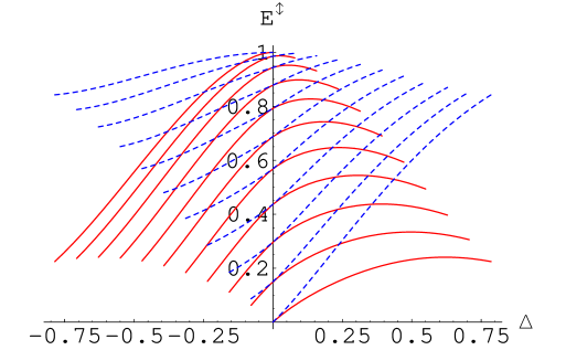
Figure 1: (color online) $E^{\uparrow}(\tau)$ (solid line) and $E^{\downarrow}(\tau)$ (dashed line) as functions of $\Delta$ for different values of $\xi$, where $p=0.5$. The highest curve corresponds to $\xi=\pi/4$. The lowest curve corresponds to $\xi=0$. Here $\Delta$ is measured in radians.

For convenience let us define $\Delta=\xi_{x}^{2}-\xi_{x}^{1}$, and denote $\xi_{x}^{1}$ simply by $\xi$, so $\xi_{x}^{2}=\xi+\Delta$. We will fix $\xi$ and analyze $E^{\uparrow}$ and $E^{\downarrow}$ for various $\Delta$. For $\Delta=0$ the map reduces to a unitary (with an appropriate capacity). As smaller angle means smaller $E^{\uparrow}(U)$, we would expect that if $U_{1}$ is mixed with $U_{2}$, where $\Delta<0$, then the entangling capacity of the resulting map will decrease relative to $E^{\uparrow}(U)$. This intuition is consistent with the results presented on Fig. 1. Similarly, we might expect that the entangling capacity of the map will increase with $\Delta>0$, and that this capacity will reach its maximum for maximal $\Delta$, i.e. maximal $E^{\uparrow}(U_{2})$. However, Fig. 1 shows that this is not the case. $E^{\uparrow}(\tau)$ indeed grows while $\Delta$ is positive and relatively small, reaching its maximum for certain intermediate positive value of $\Delta$ and then starting to decrease. In other words, if $U_{1}$ and $p$ are fixed, then maximal $E^{\uparrow}(\tau)$ is achieved for some intermediate $U_{2}$ with $\xi_{x}^{2}>\xi_{x}^{1}$, but not for $\xi_{x}^{2}=\pi/4$. This result might seem counterintuitive from the first sight, but it has a clear explanation. Let $\alpha_{1}$, $\alpha_{2}$ be the corresponding optimal values of $\alpha$ in Eq. (5) for $U_{1}$ and $U_{2}$ respectively, then the optimal value of $\alpha_{\tau}$ will lie somewhere in between, i.e. satisfy $\alpha_{1}>\alpha_{\tau}>\alpha_{2}$. For $\xi^{2}_{x}=\pi/4$, $U_{2}$ can realize its entangling capacity of 1 ebit if $\alpha_{2}=0$. However, when $U_{2}$ acts on a state with $\alpha_{\tau}>\alpha_{2}$, then it creates less than $1-H[(\cos\alpha_{\tau})^{2}]$ ebit.

Disentangling capacity, $E^{\downarrow}(\tau)$, behaves differently. It is monotonic with $\Delta$. It equals $E^{\uparrow}$ for $\Delta=0$ as expected, and it is strictly larger than $E^{\uparrow}$ for all other values of $\Delta$. The last observation shows behavior completely opposite to that of unitaries. In a sense, it is easier for non-local map to destroy entanglement rather than create it, while for unitary operations the opposite holds ent_dis_unequal .

This approach can be similarly applied to any finite number of unitaries and to continuous distribution of unitaries, which will be discussed in Section IV.3.

IV.2 Example II: Discreet DCNOT and SWAP-mixtures

For mixtures of unitaries of DCNOT and SWAP-class Method II was used. The details of numerical calculations are presented in Appendix.

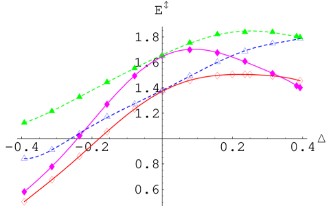
Figure 2: (color online) DCNOT: $E^{\uparrow}(\tau)$ (empty diamonds with solid line fit) and $E^{\downarrow}(\tau)$ (empty triangles with dashed line fit) as functions of $\Delta$ for $\xi_{x}^{1}=\xi_{y}^{1}=\pi/8$. SWAP: $E^{\uparrow}(\tau)$ (filled diamonds with solid line fit) and $E^{\downarrow}(\tau)$ (filled triangles with dashed line fit) as functions of $\Delta$ for $\xi_{x}^{1}=\xi_{y}^{1}=\xi_{z}^{1}=\pi/8$. In both cases $p=0.5$. Here $\Delta$ is measured in radians.

We conjectured that it is sufficient if local ancillas are qubits. Selected results are shown in Fig. 2. We can see that for DCNOT-mixture the behavior of $E^{\uparrow}(\tau)$ and $E^{\downarrow}(\tau)$ is qualitatively similar to CNOT-mixture (Fig. 1). However, for SWAP-mixture slightly different behavior is obtained. In particular $E^{\downarrow}(\tau)$ exhibits maximum at an intermediate value of $\Delta$. It is also noticeable that for $D>0.357$, $E^{\uparrow}(\tau)$ is smaller for SWAP-mixture than for DCNOT-mixture. It is a counterintuitive result that SWAP-mixture which is naturally considered as “stronger” that DCNOT-mixture has lower entangling capacity. However, again similar to the line of thought in Example I we can argue that for (relatively) large $\Delta$ the second unitary, $U_{2}$ is too strong, and therefore when it acts on the optimal state (optimal for the mixture, not for itself) it causes more destruction that corresponding $U_{2}$ of DCNOT-class would have caused.

IV.3 Example III: Entangling capacity of noisy unitary with Gaussian fluctuations

So far we analyzed discrete mixtures of unitaries. In this section we analyze a continuous distribution, which is usually what experimentalists deal with. These distributions arise due to uncertainty in one or more parameters. Such uncertainties may be caused by the limits of calibration precision of the devices and by high sensitivity of systems used to generate desired interactions. For example, the strength of exchange coupling between donors in silicon based solid-state architectures for quantum computing exhibit significant uncertainty resulting in error in gate operation silicon_CNOT: THWH .

In particular, we consider the case when a non-unitary map arises if a unitary from CNOT-class is subject to a Gaussian noise.

Recent work noisyHam analyzed the capability of noisy Hamiltonians to create entanglement. In particular, interactions of the form Eq. (8), where $\xi$ is Gaussian distributed with the mean $\overline{\xi}=\pi/4$ and standard deviation $\Omega$, were considered. Without noise this operation (CNOT operation) is able to create a maximally entangled state if it acts on a disentangled pure state. The authors analyzed the situation when the noisy operation acts on initially disentangled state, which is by itself subject to a Gaussian noise. Its capability to create entanglement was characterized in terms of the condition for inseparability of the resulting mixed state (via Peres-Horodecci separability criterion).

The aim of our analysis is different. We consider noisy interactions with $\overline{\xi}\in[0,\pi/4]$ and calculate their entangling and disentangling capacities in terms of $\overline{\xi}$ and $\Omega$. Thus, we give a comprehensive quantitative characterization of the non-local content of these noisy maps in terms of their entangling and disentangling capacities. Unlike noisyHam we do not test the resulting state on inseparability, rather calculate its distillable entanglement explicitly.

The action of a unitary $U=\exp[i\xi\sigma_{x}^{A}\sigma_{x}^{B}]$, where $\xi$ is Gaussian distributed with the mean $\overline{\xi}$ and the standard deviation $\Omega$, on the state $\rho_{AB}$ can be seen as a non-unitary CPTP map

$$\tau_{G}(\rho)\rightarrow\frac{1}{\sqrt{2\pi}\Omega}\int_{-\infty}^{+\infty}e^{-\frac{(\xi-\overline{\xi})^{2}}{2\Omega^{2}}}U\rho U^{\dagger}d\xi,$$ (10)

which is a continuous mixture of unitaries of the CNOT-class. Similarly to the Sec. IV.1 we consider pure initial state, i.e. $\rho=|\psi\rangle\!\langle\psi|$, where $\psi$ takes the form (5), calculate the distillable entanglement of the output mixed state, and maximize it over $\alpha$. Figure 3 presents numerical results for $E^{\uparrow}(\tau)$ and $E^{\downarrow}(\tau)$ as functions of $\overline{\xi}$ for several values of $\Omega$. We can see that already for $\Omega\approx 0.01~{}rad$ we obtain only very small deviation from the (dis)entangling capacity of the unitary, i.e. $\tau_{G}$ without noise - $\Omega=0$. As $\Omega$ increases the disentangling capacity increases and the entangling capacity decreases.

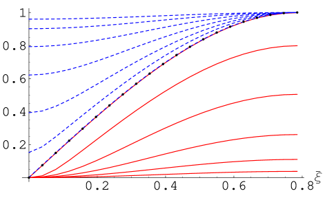
Figure 3: (color online) $E^{\uparrow}(\tau_{G})$ (solid line) and $E^{\downarrow}(\tau_{G})$ (dashed line) as a function of $\overline{\xi}$ for several values of $\Omega$: 0.01, 0.18, 0.35, 0.52, 0.69, and 0.86. The dotted line corresponds to $\Omega=0$, i.e. a unitary transformation. $\overline{\xi}$ and $\Omega$ are measured in radians.

The former fact should not be surprizing as it is known that entanglement can be destroyed even by local CPTP unital maps GPW . Thus, the more dispersed the distribution of $\xi$ becomes, the easier for $\tau_{G}$ to destroy entanglement and the harder to create it. Nevertheless, we see that even when $\Omega$ is relatively large $\tau_{G}$ is still able to create considerable amount of entanglement.

V Discussion and conclusion

We have discussed the entangling and disentangled capacities of nonlocal CPTP unital maps, i.e. maps that can be represented as probabilistic mixtures of unitaries, and have calculated these capacities in some particular cases for two qubits. Three classes of unitaries were considered, namely the CNOT, DCNOT, and SWAP classes.

We have observed that the disentangling capacity was always larger than corresponding entangling capacity, which contrasts with the unitary case where the both capacities are equal for qubits and for higher dimensions disentangling capacity cannot be greater than entangling capacity ent_dis_unequal .

In the case of the CNOT-class our results were obtained via straightforward generalization of the method for CNOT-class unitaries. We argue that the (dis)entangling capacity is achieved when a map acts on the optimal pure state from the same family as in the unitary case. Both discrete and continuous mixtures were analyzed. In the case of the DCNOT and SWAP-class direct numerical optimization was performed. We have conjectured that dimensions of the local ancillas are equal to the dimensions of the original particles, i.e. the ancillas were taken to be qubits.

A number of open question can be addressed in a future research.

It will be interesting and useful to prove (or disprove) the general conjecture that the sizes of local ancillas can be taken equal to the sizes of original particles.

Here we have calculated single-shot capacities. In the case of unitaries it had been shown that in the asymptotic regime one cannot do better BHLS_cap_Ham ; asym_ent_cap . It is important to check whether this result holds in the non-unitary case.

In the case of DCNOT and SWAP-mixtures we performed maximization over pure states only thereby obtaining lover bounds on $E^{\uparrow}(\tau)$ and $E^{\downarrow}(\tau)$, but not their actual values.

In our future research we will address the question of whether these bounds are tight. It might be the case that optimal states for these operations are mixed and, consequently, the capacities are higher than we have calculated.

Appendix A

We have used two-dimensional ancilla on each side. Consider a general state of four qubits in the tensor-product of the computational bases of the original particles $A$, $B$ and the ancillary particles $A^{\prime}$, $B^{\prime}$

$$|\Psi\rangle_{AA^{\prime}BB^{\prime}}=\sum_{i,j,k,l}c_{i,j,k,l}|i\rangle_{A}|j\rangle_{A^{\prime}}|k\rangle_{B}|l\rangle_{B^{\prime}}.$$ (11)

There are $16$ terms in the above superposition with $16$ complex amplitudes $c_{i,j,k,l}$, therefore $|\Psi\rangle$ can be parameterized using $30$ real numbers (if we take into account the global phase and normalization). We will parameterize it in the following way parametrization . First, to facilitate our analysis it is easier to incorporate four indexes $i,j,k$ and $l$, each of which runs from 0 to 1, into a single index, $x$, that runs from 1 to 16. This can be done by using the formula $x=8i+4j+2k+l+1$, which is essentially a formula for converting a number from the Boolean representation to the decimal. Second, we present amplitudes $c_{x}$ in the form

$$c_{x}=|c_{x}|e^{i\theta_{x}},$$ (12)

where $\sum_{x=1}^{16}|c_{x}|^{2}=1$ and $\theta_{1}=0$. Third, we introduce new parameters $\phi_{x}$ such that

$$c_{x}=\sin\phi_{x-1}\prod_{y=x}^{15}\cos\phi_{y},$$ (13)

where $\phi_{0}=\pi/2$. Thus the state $|\Psi\rangle$ is parameterized by 30 angles. The advantage of this parametrization is that we restrict their values only to the interval $[0,2\pi]$ that simplifies numerics.

We proceed as follows. A program generates a vector of $30$ random numbers in the interval $[0,2\pi]$. This is the initial state. We then apply the non-local map and obtain a final state. We calculate the value of the gain in entanglement $\Delta S=S(\tau(\Psi)_{BB^{\prime}})-S(\tau(\Psi)_{AA^{\prime}BB^{\prime}})-S(Tr_{AA^{\prime}}|\Psi\rangle\!\langle\Psi|)$. After that we vary the values of the random vector by a small amount and repeat these calculations again, thereby obtaining a gradient of the change in entanglement in that point. We move along the gradient to obtain the next $|\Psi\rangle$, and the procedure is repeated. Eventually, the program reaches the maximum where it stops.

References

- (1) C.H.Bennett, H.J. Bernstein, S. Popescu, B. Schumacher, Phys. Rev. A, 53 2046 (1996).
- (2) W. Dür, G. Vidal, J. I. Cirac, N. Linden, and S. Popescu, Phys. Rev. Lett. , 87, 137901 (2001).
- (3) M.S. Leifer, L. Henderson, and N. Linden, Phys. Rev. A 67, 012306 (2003).
- (4) D.W.Berry and B.C.Sanders, Phys. Rev. A 71, 022304 (2005); P.Zanardi, C. Zalka, and Lara Faoro, Phys. Rev. A 62, 030301(R) (2000); L. Clarisse, S. Ghosh, S. Severini, A. Sudbery, e-print arXiv:quant-ph/0611075v2.
- (5) C.H. Bennett, A. Harrow, D.W. Leung, and J.A. Smolin, IEEE Tran. Inf. Theory, 49, 8, 1895 (2003).
- (6) A.M. Childs, D.W. Leung, F. Verstraete, and G. Vidal, Quant. Inf. Comp. 3, 97 (2003).
- (7) N. Linden, J.A. Smolin, and A. Winter, e-print quant-ph/0511217.
- (8) M.A. Nielsen and I.L.Chuang, Quantum Computation and Quantum Information, Cambridge University Press (2004).
- (9) It was explicitly shown lhl that the optimization can be restricted to pure states.
- (10) B. Kraus and J.I. Cirac, Phys. Rev. A 63, 062309 (2001).
- (11) W.K. Wootters, Phys. Rev. Lett. 80, 2245 (1998).
- (12) C.H. Bennett, D.P. DiVincenzo, J.A. Smolin, and W.K. Wootters, Phys. Rev. A 54, 3824 (1996).
- (13) J. I. Cirac, W. Dür, B. Kraus and M. Lewenstein, Phys. Rev. Lett. , 86, 544 (2001); W. Dür and J. I. Cirac, Phys. Rev. A, 64, 012317 (2001).
- (14) B. Kraus and J.I. Cirac, Phys. Rev. A 63, 062309 (2001).
- (15) Strictly speaking DCNOT-class and SWAP-class should be unified under a single class if analyzed according to the criteria of interconvertability under LOCC U->U . In the framework of (dis)entangling capacity it is useful to identify them as separate classes, because their behavior differs qualitatively.
- (16) W. Dür, G. Vidal, J. I. Cirac, Phys. Rev. Lett. , 89, 057901 (2002).
- (17) V. Vedral and M. B. Plenio, Phys. Rev. A 57, 1619 (1998).
- (18) Here we assume that all unitaries in Eq. (1) belong to the same class, which is typical for real situations where only parameters of the coupling are subject to variations.
- (19) M. J. Testolin, C. D. Hill, C. J. Wellard, L. C. L. Hollenberg, e-print quant-ph/0701165.
- (20) S. Bandyopadhyay and D.A. Lidar, Phys. Rev. A 70, 010301(R) (2004).
- (21) B.Groisman, S. Popescu, and A. Winter, Phys. Rev. A72, 032317 (2005).
- (22) This method is a partial adaptation of the method used in Ref. VP:ent_m_pp for calculation the relative entropy of entanglement.