Higher Dimensional Conundra

Steven G. Krantz

Abstract: In recent years, especially in the subject of harmonic analysis, there has been interest in geometric phenomena of ${\tenmsb R}^{N}$ as $N\rightarrow+\infty$. In the present paper we examine several specific geometric phenomena in Euclidean space and calculate the asymptotics as the dimension gets large.

0 Introduction

Typically when we do geometry we concentrate on a specific venue in a particular space. Often the context is Euclidean space, and often the work is done in ${\tenmsb R}^{2}$ or ${\tenmsb R}^{3}$. But in modern work there are many aspects of analysis that are linked to concrete aspects of geometry. And there is often interest in rendering the ideas in Hilbert space or some other infinite dimensional setting. Thus one wants to see how the finite-dimensional result in ${\tenmsb R}^{N}$ changes as $N\rightarrow+\infty$.

In the present paper we study some particular aspects of the geometry of ${\tenmsb R}^{N}$ and their asymptotic behavior as $N\rightarrow\infty$. We choose these particular examples because the results are surprising or especially interesting. One may hope that they will lead to further studies.

1 Volume in ${\tenmsbb R}^{N}$

Let us begin by calculating the volume of the unit ball in ${\tenmsb R}^{N}$ and the surface area of its bounding unit sphere. We let $\Omega_{N}$ denote the former and $\omega_{N-1}$ denote the latter. In addition, we let $\Gamma(x)$ be the celebrated Gamma function of L. Euler. It is a helpful intuition (which is literally true when $x$ is an integer) that $\Gamma(x)\approx(x-1)!$. We shall also use Stirling’s formula which says that

$$k!\approx k^{k}\cdot e^{-k}\cdot\sqrt{2\pi k}$$

or, more generally,

$$\Gamma(x)\approx(x-1)^{x-1}e^{-(x-1)}\sqrt{2\pi(x-1)}$$

for $x\in{\tenmsb R}$, $x>0$.

Lemma 1

We have that

$$\int_{{\tenmsb R}^{N}}e^{-\pi\|{\bf x}\|^{2}}\,d{\bf x}=1.$$

Proof: The case $N=1$ is familiar from calculus. We write

$$S=\int_{\tenmsb R}e^{-\pi t^{2}}\,dt$$

hence

$$S^{2} = \int_{\tenmsb R}e^{-\pi x^{2}}\,dx\int_{\tenmsb R}e^{-\pi y^{2}}\,dy$$

$$= \mathop{\int\!\!\!\int}_{{\tenmsb R}^{2}}e^{-\pi\|{\bf x}\|^{2}}d{\bf x}$$

$$\stackrel{{\scriptstyle\rm(polar\ coordinates)}}{{=}} \int_{0}^{\infty}\int_{\|{\bf x}\|=1}e^{-\pi r^{2}}r\,ds({\bf x})dr$$

$$= \omega_{1}\frac{1}{2\pi}e^{-\pi r^{2}}\biggr{|}_{0}^{\infty}$$

$$= \frac{\omega_{1}}{2\pi}$$

$$= 1$$

hence $S=1$.

For the $N-$dimensional case, write

$$\int_{{\tenmsb R}^{N}}e^{-\pi|x|^{2}}dx=\int_{{\tenmsb R}}e^{-\pi x_{1}^{2}}dx_{1}\cdots\int_{{\tenmsb R}}e^{-\pi x_{N}^{2}}dx_{N}$$

and apply the one-dimensional result. $\mathord{{\vrule height=6.0pt,depth=0.4pt,width=0.4pt\vrule height=0.0pt,depth=0.4pt,width=6.0pt\hbox to0.0pt{\hss\vrule height=6.0pt,depth=-5.6pt,width=6.4pt}\hskip-0.4pt\vrule height=6.0pt,depth=0.4pt,width=0.4pt}}\;$

Let $\sigma$ be the unique rotationally invariant area measure on $S_{N-1}=\partial B_{N}$.

Lemma 2

We have

$$\omega_{N-1}=\frac{2\pi^{N/2}}{\Gamma(N/2)}\,.$$

Proof:    Introducing polar coordinates we have

$$1=\int_{{\tenmsb R}^{N}}e^{-\pi|x|^{2}}dx=\int_{S^{N-1}}d\sigma\int_{0}^{\infty}e^{-\pi r^{2}}r^{N-1}dr$$

or

$$\frac{1}{\omega_{N-1}}=\int_{0}^{\infty}e^{-\pi r^{2}}r^{N}\frac{dr}{r}.$$

Letting $s=r^{2}$ in this last integral and doing some obvious manipulations yields the result. $\mathord{{\vrule height=6.0pt,depth=0.4pt,width=0.4pt\vrule height=0.0pt,depth=0.4pt,width=6.0pt\hbox to0.0pt{\hss\vrule height=6.0pt,depth=-5.6pt,width=6.4pt}\hskip-0.4pt\vrule height=6.0pt,depth=0.4pt,width=0.4pt}}\;$

Corollary 3

The volume of the unit ball in ${\tenmsb R}^{N}$ is

$$\Omega_{N}=\frac{\omega_{N-1}}{N}=\frac{2\pi^{N/2}}{\Gamma(N/2)\cdot N}\,.$$

Proof: We calculate that

$$\Omega_{N}=\mathop{\int\!\!\!\int}_{B}1\,dV(x)\stackrel{{\scriptstyle\rm(polar\ coordinates)}}{{=}}\int_{0}^{1}\int_{\|{\bf x}\|=1}1\cdot r^{N-1}\,d\sigma({\bf x})dr=\omega_{N-1}\cdot\frac{r^{N}}{N}\biggr{|}_{0}^{1}=\frac{\omega_{N-1}}{N}\,.$$

That completes the proof. $\mathord{{\vrule height=6.0pt,depth=0.4pt,width=0.4pt\vrule height=0.0pt,depth=0.4pt,width=6.0pt\hbox to0.0pt{\hss\vrule height=6.0pt,depth=-5.6pt,width=6.4pt}\hskip-0.4pt\vrule height=6.0pt,depth=0.4pt,width=0.4pt}}\;$

Now the first nontrivial fact that we wish to observe about the volume of the Euclidean unit ball in $N$-space is that that volume tends to 0 at $N\rightarrow\infty$. More formally,

Proposition 4

We have the limit

$$\lim_{N\rightarrow+\infty}\Omega(N)=0\,.$$

Proof: We calculate that

(Volume of Unit Ball) $$= \frac{2\pi^{N/2}}{\Gamma(N/2)\cdot N}$$

$$\approx \frac{2\pi^{N/2}}{((N-2)/2)^{(N-2)/2}e^{-(N-2)/2}\sqrt{2\pi[(N-2)/2]}\cdot N}$$

$$\approx \frac{(2\pi e)^{N/2}\cdot 2}{N^{(N-1)/2}\cdot\sqrt{\pi}\cdot N}$$

$$\approx \frac{(2\pi e)^{N/2}\cdot 2}{N^{(N+1)/2}\cdot\sqrt{\pi}}$$

$$\approx \left(\frac{2\pi e}{N}\right)^{N/2}\cdot\frac{1}{\sqrt{N}}\cdot\frac{2}{\sqrt{\pi}}\,.$$

This expression clearly tends to 0 as $N\rightarrow+\infty$. $\mathord{{\vrule height=6.0pt,depth=0.4pt,width=0.4pt\vrule height=0.0pt,depth=0.4pt,width=6.0pt\hbox to0.0pt{\hss\vrule height=6.0pt,depth=-5.6pt,width=6.4pt}\hskip-0.4pt\vrule height=6.0pt,depth=0.4pt,width=0.4pt}}\;$

In fact we can actually say something about the rate at which the volume of the ball tends to zero. We have

Proposition 5

We have the estimate

$$0\leq\Omega_{N}\leq 2\cdot\frac{20^{N/2}}{N^{(N+1)/2}}\,.$$

Proof: Follows by inspection of the last line of the proof of Proposition 4. $\mathord{{\vrule height=6.0pt,depth=0.4pt,width=0.4pt\vrule height=0.0pt,depth=0.4pt,width=6.0pt\hbox to0.0pt{\hss\vrule height=6.0pt,depth=-5.6pt,width=6.4pt}\hskip-0.4pt\vrule height=6.0pt,depth=0.4pt,width=0.4pt}}\;$

In fact something more is true about the volumes of balls in high-dimensional Euclidean space.

Proposition 6

Let $R>0$ be fixed. Then

$$\lim_{N\rightarrow+\infty}\hbox{Vol}(B(0,R))=0\,.$$

In other words, the volume of the ball of radius $R$ tends to 0.

Proof: From the formula for the volume of the unit ball we have that

$$\lim_{N\rightarrow+\infty}\hbox{Vol}(B(0,R))=\lim_{N\rightarrow+\infty}\left(\frac{2\pi eR^{2}}{N}\right)^{N/2}\cdot\frac{1}{\sqrt{N}}\cdot\frac{2}{\sqrt{\pi}}\,.$$

This expression clearly tends to 0 as $N\rightarrow+\infty$. $\mathord{{\vrule height=6.0pt,depth=0.4pt,width=0.4pt\vrule height=0.0pt,depth=0.4pt,width=6.0pt\hbox to0.0pt{\hss\vrule height=6.0pt,depth=-5.6pt,width=6.4pt}\hskip-0.4pt\vrule height=6.0pt,depth=0.4pt,width=0.4pt}}\;$

We leave the proof of the next result as an exercise for the reader; simply examine the formula for $\omega_{N-1}$:

Proposition 7

Let $R>0$. Then the surface area of the sphere of radius $R$ in ${\tenmsb R}^{N}$ tends to 0 as $N\rightarrow+\infty$.

The following very simple but remarkable fact comes up in considerations of spherical summation of Fourier series.

Proposition 8

As $N\rightarrow+\infty$, the volume of the unit ball in ${\tenmsb R}^{N}$ is concentrated more and more out near the boundary sphere. More precisely, let $\delta>0$. Then

$$\lim_{N\rightarrow+\infty}\frac{\hbox{\rm volume}(B(0,1)\setminus B(0,1-\delta))}{\hbox{\rm volume}(B(0,1)}=1\,.$$

Proof: We have

$$\lim_{N\rightarrow+\infty}\frac{\hbox{\rm volume}(B(0,1)\setminus B(0,1-\delta))}{\hbox{\rm volume}(B(0,1)} = \lim_{N\rightarrow+\infty}\frac{[1-(1-\delta)^{N}]\cdot[2\pi^{N/2}]/[\Gamma(N/2)\cdot N]}{[2\pi^{N/2}]/[\Gamma(N/2)\cdot N]}$$

$$= \lim_{N\rightarrow+\infty}1-(1-\delta)^{N}$$

$$= 1\,.$$

That is the desired conclusion. $\mathord{{\vrule height=6.0pt,depth=0.4pt,width=0.4pt\vrule height=0.0pt,depth=0.4pt,width=6.0pt\hbox to0.0pt{\hss\vrule height=6.0pt,depth=-5.6pt,width=6.4pt}\hskip-0.4pt\vrule height=6.0pt,depth=0.4pt,width=0.4pt}}\;$

2 A Case of Leakage

The title of this section gives away the punchline of the example. Or so it may seem to some.

Consider at first a square box of side two with sides parallel to the coordinate axes in the Euclidean plane. We may inscribe in this box four discs of diameter 1, as shown in Figure 1. These discs will be called primary discs. Once those four discs are inscribed, we may inscribe a small, shaded disc in the middle as shown in Figure 2. We set

$${\cal R}_{2}=\frac{\hbox{area\ of\ shaded\ disc}}{\hbox{area\ of\ large\ box}}\,.$$

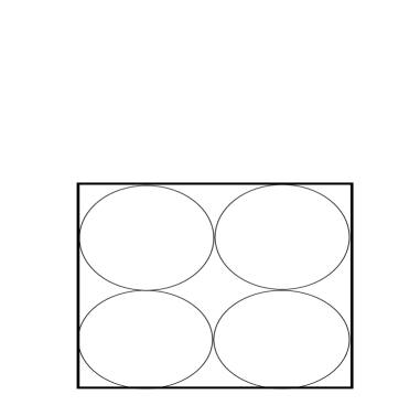
Figure 1: The configuration in dimension 2.

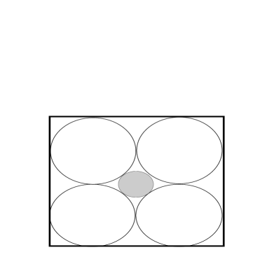
Figure 2: The shaded disc in dimension 2.

The same construction may be performed in Euclidean dimension 3. Examine Figure 3. It suggests a rectangular parallelepiped with all sides equal to 2, and 8 unit balls inscribed inside in a canonical fashion. These eight primary balls determine a unique inscribed shaded ball in the center. We set

$${\cal R}_{3}=\frac{\hbox{volume\ of\ shaded\ ball}}{\hbox{volume\ of\ large\ box}}\,.$$

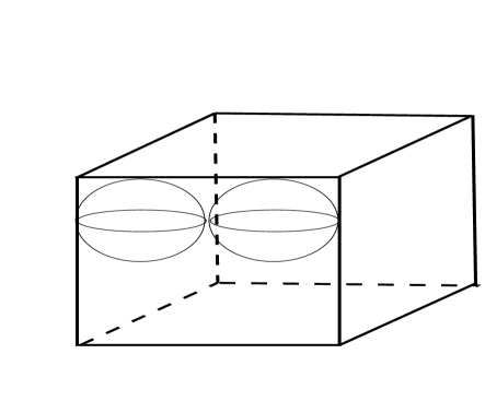
Figure 3: The configuration in dimension 3.

A similar construction may be performed in any dimension $N\geq 2$, with $2^{N}$ balls inscribed in a rectangular box of side 2. The ratio ${\cal R}_{N}$ is then calculated in just the same way. The question is then

What is the limit   $\lim_{N\rightarrow\infty}{\cal R}_{N}$  as  $N\rightarrow+\infty$?

It is natural to suppose, and most people do suppose, and that this limit (assuming it exists) is between 0 and 1. All other things being equal, it is likely equal to either 0 or 1. Thus it comes as something of a surprise that this limit is in fact equal to $+\infty$. Let us now enunciate this result and prove it.

Proposition 9

The limit

$$\lim_{N\rightarrow+\infty}{\cal R}_{N}=+\infty\,.$$

Of course this result is counter-intuitive, because we all instinctively believe that the shaded ball, in any dimension, is contained inside the big box. Such is not the case. We are being fooled by the 2-dimensional situation depicted in Figure 1. In that special situation, any of the two adjacent primary discs actually touch in such a way as to trap the shaded disc in a particular convex subregion of the big box (see Figure 4). So certainly it must be that ${\cal R}_{2}<1$. But such is not the case in higher dimensions. There is actually a gap on each side of the box through which the shaded ball can leak. And indeed it does.

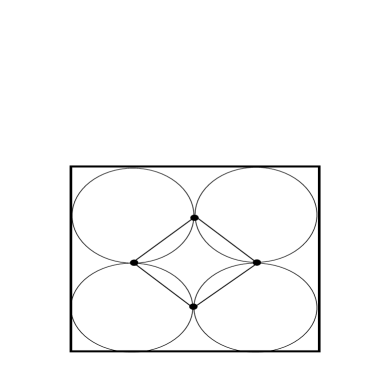
Figure 4: The disc trapped in dimension 2.

This is what we shall now show. First we shall perform the calculation of ${\cal R}_{N}$ for each $N$ and confirm that the expression tends to $+\infty$ as $N\rightarrow+\infty$. Then we shall calculate the first dimension in which the shaded ball actually leaks out of the box.

Proof of the Proposition: Notice that the center of one of the primary balls is at the point $(1,1,\dots,1)$. It is a simple matter to calculate that a boundary point of this ball that is nearest to the center of the box is located at $P^{*}\equiv(1-1/\sqrt{N},1-1/\sqrt{N},\dots,1-1/\sqrt{N}$. Since the shaded ball will osculate the primary ball at that point, we see that the shaded ball has center the origin and radius equal to

$$\hbox{dist}(0,P^{*})=\sqrt{(1-1/\sqrt{N})^{2},1-1/\sqrt{N})^{2},\dots,1-1/\sqrt{N})^{2}}=\sqrt{N+1-2\sqrt{N}}\,.$$

Thus we see that the volume of the shaded ball is

$$[N+1-2\sqrt{N}]^{N/2}\cdot\Omega_{N}\,.$$

The ratio ${\cal R}_{N}$ is then

$${\cal R}_{N}=\frac{[N+1-2\sqrt{N}]^{N/2}\cdot\Omega_{N}}{2^{N}}\,.$$

Now we may simplify this last expression to

$${\cal R}_{N}=\frac{2\cdot\pi^{N/2}}{\Gamma(N/2)\cdot N}\cdot\frac{[N+1-2\sqrt{N}]^{N/2}}{2^{N}}\,.$$

After some simplification we find that

$${\cal R}_{N}=\frac{2(\pi/4)^{N/2}\cdot[N+1-2\sqrt{N}]^{N/2}}{\Gamma(N/2)\cdot N}\,.$$

By Stirling’s formula, this last expression is approximately equal to

$$\frac{2\cdot(\pi/4)^{N/2}(N+1-2\sqrt{N})^{N/2}}{N}\cdot\left(\frac{N-2}{2}\right)^{(2-N)/2}\cdot e^{(N-2)/2}\cdot\frac{1}{\sqrt{\pi(N-2)}}$$

$$= \frac{2}{N}\left[\frac{\pi}{4}(N+1-2\sqrt{N})\cdot\frac{2}{N-2}\cdot e\right]^{N/2}\cdot\frac{N-2}{2}\cdot\frac{1}{\sqrt{\pi(N-2)}}\cdot\frac{1}{e}\,.$$

After some manipulation, we finally find that

$$\lim_{N\rightarrow\infty}{\cal R}_{N} = \lim_{N\rightarrow\infty}\frac{2}{N}\left(\frac{\pi e}{2}\right)^{N/2}\cdot\left(\frac{N+1}{N-2}\right)^{N/2}\cdot\frac{N-2}{2}\cdot\frac{1}{\sqrt{\pi(N-2)}}\cdot\frac{1}{e}$$

$$= \lim_{N\rightarrow\infty}\frac{2}{N}\left(\frac{\pi e}{2}\right)^{N/2}\left(1+\frac{3}{N-2}\right)^{N/2}\cdot\frac{N-2}{2}\cdot\frac{1}{\sqrt{\pi(N-2)}}\cdot\frac{1}{e}\,.$$

Now, in the limit, we may replace expressions like $N-2$ by $N$. And we may reparametrize $N$ as $3N$. The result is

$$\lim_{N\rightarrow\infty}\frac{2}{N}\left(\frac{\pi e}{2}\right)^{N/2}\cdot\left(1+\frac{3}{N}\right)^{N/2}\cdot\frac{N-2}{2}\cdot\frac{1}{\sqrt{\pi(N-2)}}\cdot\frac{1}{e}$$

$$= \lim_{N\rightarrow\infty}\frac{2}{N}\left(\frac{\pi e}{2}\right)^{N/2}\cdot\left(1+\frac{1}{N}\right)^{3N/2}\cdot\frac{N-2}{2}\cdot\frac{1}{\sqrt{\pi(N-2)}}\cdot\frac{1}{e}$$

$$= \lim_{N\rightarrow\infty}\frac{2}{N}\cdot\left(\frac{\pi e}{2}\right)^{N/2}\left[\left(1+\frac{1}{N}\right)^{N}\right]^{3/2}\cdot\frac{N-2}{2}\cdot\frac{1}{\sqrt{\pi(N-2)}}\cdot\frac{1}{e}\,.$$

What we see now is that this last equals

$$\lim_{N\rightarrow\infty}\left(\frac{\pi e}{2}\right)^{N/2}\cdot\frac{1}{\sqrt{N}}\cdot\frac{e^{1/2}}{\sqrt{\pi}}\,.$$

Plainly, because $\pi e/2>4$, this limit is $+\infty$. That proves the result. $\mathord{{\vrule height=6.0pt,depth=0.4pt,width=0.4pt\vrule height=0.0pt,depth=0.4pt,width=6.0pt\hbox to0.0pt{\hss\vrule height=6.0pt,depth=-5.6pt,width=6.4pt}\hskip-0.4pt\vrule height=6.0pt,depth=0.4pt,width=0.4pt}}\;$

And now we turn to the question of when the shaded ball starts to leak out of the big box. This is in fact easy to analyze. We need only determine when the radius of the shaded ball exceeds 1. First notice that the radius of the shaded ball is monotone increasing in $N$. Now we need to solve

$$\sqrt{N+1-2\sqrt{N}}>1\,.$$

This is a simple algebra problem, and the solution is $N>4$. Thus, beginning in dimension 5, the shaded ball will “leak out of” the large box.

It may be noted that Richard W. Cottle has made a study of mathematical phenomena that change (in the manner of a catastrophe—see [ZEE]) between dimensions 4 and dimensions 5. The results may be found in [COT].

3 Centroids

This final section of the paper will be more like an invitation to further exploration. We cannot include all the details of the calculations, as they are too recondite and complex. Yet the topic is very much in the spirit of the theme of this paper, and we cannot resist including a few pointers to this new and interesting work (for which see [KRA1] and [KRMP]).

The inspiration for this work is the following somewhat surprising observation. Let $T$ be a triangle in the plane (see Figure 5). There are three ways to calculate the centroid of this figure: (i) average the vertices, (ii) average the edges, or (iii) average the 2-dimensional solid figure. And the question is: are these three versions of the centroid the same? The answer is that (i) and (iii) are always the same. Generically (ii) is different. In fact the three versions of the centroid coincide if and only if the triangle is equilateral [KRMP].

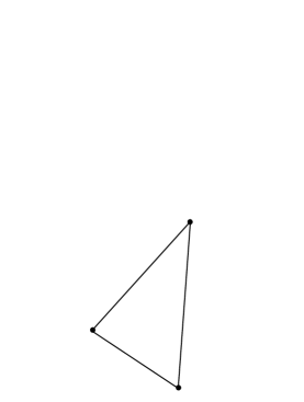
Figure 5: Centroids for a triangle.

We used this fact as a springing-off point to investigate analogous questions in higher dimensions. Consider the simplex S in ${\tenmsb R}^{N}$ that is the convex hull of the points $0=(0,0,\dots,0)$, $(1,0,\dots,0)$, $(0,1,0,\dots,0)$, …, $(0,0,\dots,0,1)$. Refer to Figure 6. Such an $N$-dimensional geometric figure comes equipped with $(N+1)$ notions of centroid: one can average the vertices (or 1-dimensional skeleton) ${\cal S}_{0}$, or one can average over the 1-dimensional skeleton ${\cal S}_{1}$, or one can average over the two-dimensional skeleton ${\cal S}_{2}$A, or …one can average over the $(N-1)$-dimensional skeleton ${\cal S}_{N-1}$, or one can average over the $N$-dimensional solid ${\cal S}_{N}$. There results the centroids ${\cal C}_{0,N}$, ${\cal C}_{1,N}$, …, ${\cal C}_{N,N}$. And the question is: Are these different notions of centroid all the same? And here is the somewhat surprising answer:

In dimensions 2 through 12 (for the ambient space), the skeletons ${\cal S}_{0}$ and ${\cal S}_{N}$ for the simplex S have the same centroid. In those same dimensions, the skeletons ${\cal S}_{1}$, ${\cal S}_{2}$, …, ${\cal S}_{N-1}$ all have different centroids, and the centroids all differ from the common centroid for ${\cal S}_{0}$ and ${\cal S}_{N}$. But in dimension 13 things are different. In fact in that dimension the skeletons ${\cal S}_{3}$ and ${\cal S}_{8}$ have the same centroid.

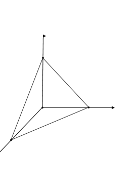
Figure 6: A simplex in ${\tenmsb R}^{N}$.

Let us say a word about why these facts are true. Let ${\bf e}_{j}$ denote the $j^{\rm th}$ coordinate vector in ${\tenmsb R}^{N}$ (i.e., the vector with a 1 in the $j^{\rm th}$ position and 0s in all other slots). Then a sophisticated computation with elementary calculus yields that the centroid of the $k$-skeleton ${\cal S}_{k}$ of the simplex which is the convex hull of $0,{\bf e}_{1},{\bf e}_{2},\dots,{\bf e}_{N}$ is

$${\cal C}_{k,N}=\frac{1}{N}\cdot\frac{k+(N-k)\sqrt{k+1}}{(k+1)+(N-k)\sqrt{k+1}}({\bf e}_{1}+{\bf e}_{2}+\cdots+{\bf e}_{N})\,.$$

From this formula it can immediately be verified that

$${\cal S}_{0}={\cal S}_{N}=\frac{1}{N+1}({\bf e}_{1}+{\bf e}_{2}+\cdots+{\bf e}_{N})\,.$$

It can also be checked that, in dimensions 2 through 12, all the intermediate skeletons have distinct centroids. But, in dimension $N=13$, we observe that

$${\cal C}_{3,13}={\cal C}_{8,13}=\frac{23}{13\cdot 24}({\bf e}_{1}+{\bf e}_{2}+\cdots+{\bf e}_{N})\,.$$

One may well ask whether dimension $N=13$ is the only dimension in which there are two intermediate skeletons with the same centroid. The answer is “no”; there are in fact infinitely many such dimensions (although they are quite sparse—sparser than the prime integers). One may verify this assertion by using the following Diophantine formula.

Theorem 10

Fix a dimension $N\geq 2$. Consider the simplex S as described above. There are skeletons of dimension $k_{1}$ and $k_{2}$, $1\leq k_{1}<k_{2}\leq N-1$, of the simplex S which have the same centroid if and only if $k_{1}=a^{2}-1$, $k_{2}=b^{2}-1$ (for positive integers $a$ and $b$) and, in addition,

$$N=(b^{2}+ab+a^{2})-(b+a)-1\,.$$

Obviously this theorem gives us a tool for finding dimensions in which the simplex S has two intermediate skeletons with the same centroid. The following table gives some values of the dimension, and of the intermediate dimensions of skeletons which have the same centroid. Of course this data may be confirmed by direct calculation with the formula $(\star)$. We stress that there are in fact infinitely many dimensions in which this phenomenon occurs. The proof of this statement is a nontrivial exercise in elementary number theory (see [KRMP]).

$$\begin{array}[]{|c|c|c|c|}\hline\cr\hbox{\bf value of \boldmath$N$}&\hbox{\bf value of \boldmath$k_{1}$}&\hbox{\bf value of \boldmath$k_{2}$}&\hbox{\bf approx.\ coord.\ of centroid}\\ \hline\cr\hline\cr 13&3&8&0.0737179487\\ 21&3&15&0.0464285714\\ 29&8&15&0.0340038314\\ 31&3&24&0.0317204301\\ 40&8&24&0.0247619047\\ 43&3&35&0.0229789590\\ 51&15&24&0.0194852941\\ 53&8&35&0.0187368973\\ 57&3&48&0.0173872180\\ 65&15&35&0.0153133903\\ \hline\cr\end{array}$$

We conclude this discussion by recording the fact that it is impossible in any dimension for there to be three intermediate skeletons with the same centroid.

Proposition 11

For no dimension $N$ can there exists 3 distinct number $1\leq k_{1}<k_{2}<k_{3}\leq N-1$ such that the centroids ${\cal C}_{k_{1},N}$, ${\cal C}_{k_{2},N}$, ${\cal C}_{k_{3},N}$ for the simplex S coincide.

Proof: We let

$$Q(a,b)=(b^{2}+ab+a^{2})-(b+a)-1\,.$$

It suffices for us to show that there do not exist natural numbers $a<b<c$ such that $Q(a,b)=Q(a,c)$. Seeking a contradiction, we suppose that such a triple does indeed exist.

Then

$$b^{2}+ab-b=c^{2}+ac-c$$

or

$$b^{2}+(a-1)b=c^{2}+(a-1)c\,.$$

Since $a\geq 1$, the function $b\mapsto b^{2}+(a-1)b$ is strictly increasing, which yields a contradiction. $\mathord{{\vrule height=6.0pt,depth=0.4pt,width=0.4pt\vrule height=0.0pt,depth=0.4pt,width=6.0pt\hbox to0.0pt{\hss\vrule height=6.0pt,depth=-5.6pt,width=6.4pt}\hskip-0.4pt\vrule height=6.0pt,depth=0.4pt,width=0.4pt}}\;$

The exploration of centroids for simplices of high dimension is a new venue of exploration. There are many new phenomena, and more to be discovered. See [KRMP] for more results along these lines. The reference [ZON] is also of interest.

References

1. R. W. Cottle, Quartic barriers, Computational Optimization and Applications 12(1999), 81–105.

2. S. G. Krantz, A Matter of gravity, Amer. Math. Monthly 110(2003), 465–481.

3. S. G. Krantz, J. E. McCarthy, and H. R. Parks, Geometric characterizations of centroids of simplices, Journal of Mathematical Analysis and Applications 316(2006), 87–109.

4. E. C. Zeeman, Catastrophe Theory. Selected Papers, 1972–1977, Addison-Wesley, Reading, MA, 1977.

5. C. Zong, Strange Phenomena in Convex and Discrete Geometry, Springer-Verlag, New York, 1996.

STEVEN G. KRANTZ received his B.A. degree from the University of California at Santa Cruz in 1971. He earned the Ph.D. from Princeton University in 1974. He has taught at UCLA, Princeton University, Penn State, and Washington University in St. Louis. Krantz is the holder of the UCLA Alumni Foundation Distinguished Teaching Award, the Chauvenet Prize, and the Beckenbach Book Prize. He is the author of 150 papers and 50 books. His research interests include complex analysis, real analysis, harmonic analysis, and partial differential equations. Krantz is currently the Deputy Director of the American Institute of Mathematics.
American Institute of Mathematics, 360 Portage Avenue,
Palo Alto, CA 94306
skrantz@aimath.org