Cross-Layer Optimization of MIMO-Based Mesh Networks with Gaussian Vector Broadcast Channels

Abstract

MIMO technology is one of the most significant advances in the past decade to increase channel capacity and has a great potential to improve network capacity for mesh networks. In a MIMO-based mesh network, the links outgoing from each node sharing the common communication spectrum can be modeled as a Gaussian vector broadcast channel. Recently, researchers showed that “dirty paper coding” (DPC) is the optimal transmission strategy for Gaussian vector broadcast channels. So far, there has been little study on how this fundamental result will impact the cross-layer design for MIMO-based mesh networks. To fill this gap, we consider the problem of jointly optimizing DPC power allocation in the link layer at each node and multihop/multipath routing in a MIMO-based mesh networks. It turns out that this optimization problem is a very challenging non-convex problem. To address this difficulty, we transform the original problem to an equivalent problem by exploiting the channel duality. For the transformed problem, we develop an efficient solution procedure that integrates Lagrangian dual decomposition method, conjugate gradient projection method based on matrix differential calculus, cutting-plane method, and subgradient method. In our numerical example, it is shown that we can achieve a network performance gain of $34.4\%$ by using DPC.

I Introduction

Since Telatar’s [1] and Foschini’s [2] pioneering works predicting the potential of high spectral efficiency provided by multiple antenna systems, the last decade has witnessed a soar of research activity on Multiple-Input Multiple-Output (MIMO) technologies. The benefits of substantial improvements in wireless link capacity at no cost of additional spectrum and power have quickly positioned MIMO as one of the breakthrough technologies in modern wireless communications, rendering it as an enabling technology for next generation wireless networks. However, applying MIMO in wireless mesh networks (WMNs) is not a trivial technical extension. With the increased number of antennas at each node, interference is likely to become stronger if power level at each node, power allocation to each antenna element, and routing are not managed wisely. As a result, cross-layer design is necessary for MIMO-based WMNs.

In a MIMO-based WMN, the set of outgoing links from a node sharing a common communication spectrum can be modeled as a nondegraded Gaussian vector broadcast channel, for which the capacity region is notoriously hard to analyze [3]. In the networking literature, most works considering links sharing a common communication spectrum are concerned with how to allocate frequency sub-bands/time-slots and schedule transmissions to efficiently share the common communication spectrum. As an example, Fig. 1(a) shows a simple broadcast channel where there are three uncoordinated users and a single transmitting node. Suppose that messages $x$, $y$, and $z$ need to be delivered to user 1, user 2, and user 3, respectively. Also, suppose that the received signals subject to ambient noise are $\hat{x}$, $\hat{y}$, and $\hat{z}$, and the decoding functions are $f_{1}(\cdot)$, $f_{2}(\cdot)$, and $f_{3}(\cdot)$, respectively. The conventional strategy is to divide a unit time frame into three time slots (or divide a unit band into three sub-bands) $\tau_{1}$, $\tau_{2}$, and $\tau_{3}$, and then find the optimal scheduling for transmissions to users 1, 2 and 3, accordingly. The major benefit of this strategy is that interference can be eliminated.

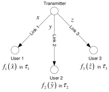
(a) Time or frequency division

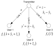
(b) DPC transmission strategy

Figure 1: A 3-user broadcast channel example.

Although the time or frequency division schemes are simple and effective, they are not necessarily the smartest strategy. In fact, Cover had shown in his classical paper [4] that the transmission scheme jointly encoding all receivers’ information at the transmitter can do strictly better in broadcast channels. However, the capacity achieving transmission signaling scheme for general nondegraded Gaussian vector broadcast channels is very difficult to determine and has become one of the most basic questions in network information theory [3]. Very recently, significant progress has been made in this area. Most notably, Weigarten et. al. finally proved the long-open conjecture that the “dirty paper coding” strategy (DPC) [5] is the optimal transmission scheme for Gaussian vector broadcast channels [6] in the sense that the DPC rate region $\mathcal{C}_{\mathrm{DPC}}$ of a broadcast channel is equal to the broadcast channel’s capacity region $\mathcal{C}_{\mathrm{BC}}$, i.e., $\mathcal{C}_{\mathrm{BC}}=\mathcal{C}_{\mathrm{DPC}}$. However, this fundamental result is still not adequately exposed to the networking research community. So far, how to exploit DPC’s benefits in the cross-layer design for wireless mesh networks has not yet been studied in the literature. The main objective of this study is to fill this gap and to obtain a rigorous and systematic understanding of the impact of applying DPC to the cross-layer optimization for MIMO-based mesh networks.

To begin with, it is beneficial to introduce the basic idea of DPC, which turns out to be very simple. For the same 3-user example, consider the following strategy as shown in Fig. 1(b). We first jointly encode the messages for all the users in a certain order and then broadcast the resulting codeword simultaneously. Suppose that we pick user 1 to be encoded first, then followed by user 2, and finally user 3. We choose the codeword $x$ for user 1 as before. Then, the interference seen by user 2 due to user 1 (denoted by $\hat{x}_{2}$) is known at the transmitter. So, the transmitter can subtract the interference and encode user 2 as $y^{\prime}=y-\hat{x}_{2}$ rather than $y$ itself. As a result, user 2 does not see any interference from the signal intended for user 1. Likewise, after encoding user 2, the interferences seen by user 3 due to user 1 and 2 (denoted by $\hat{x}_{3}$ and $\hat{y}_{3}$) are known at the transmitter. Then, the transmitter can subtract the interferences and encode user 3 as $z^{\prime}=z-\hat{x}_{3}-\hat{y}_{3}$ rather than $z$ itself. Therefore, user 3 does not see any interferences from the signals intended for user 1 and 2. In the end, the transmitter adds all the codewords together and broadcasts the sum to all users simultaneously. As a result, it is easy to see from Fig. 1(b) that the received signal at user 1 is $\hat{x}+\hat{y}_{1}+\hat{z}_{1}$, i.e., user 1 will experience the interference from the signals intended for users 2 and 3; the received signal at user 2 is $\hat{y}+\hat{z}_{2}$, i.e., user 2 only experiences the interference from the signal intended for user 3; and finally, the received signal at user 3 is $\hat{z}$, i.e., user 3 does not experience any interference. This process operates like writing on a dirty paper, hence the name. Although counterintuitive, the capacity region of DPC that allows interference is strictly larger than those of time or frequency division schemes.

After understanding what DPC is, one may ask two very natural and interesting questions:

1. How will the enlarged capacity region at each node due to DPC impact the network performance in the upper layers?

2. Are there any new challenges if DPC is employed in a MIMO-based networking environment?

Notice that, when DPC is employed, the encoding order plays a critical role. For a $K$-user broadcast channel, there exists $K!$ permutations. Also, since DPC allows interference among the users, power allocation among different users along with the encoding order has a significant impact on the system performance. As we show later, the DPC link rates in a broadcast channel are non-connvex functions. Thus, even the optimization for a single $K$-user Gaussian vector broadcast channel is a very challenging combinatorial non-convex problem, not to mention the cross-layer design in a networking environment with multiple broadcast channels.

In this paper, we aim to solve the problem of jointly optimizing DPC per-antenna power allocation at each node in the link layer and multihop/multipath routing in a MIMO-based WMN. Our contributions are three-fold. First, this paper is the first work that studies the impacts of applying DPC to the cross-layer design for MIMO-based WMNs. In our numerical example, it is shown that we can achieve a network performance gain of $34.4\%$ by using DPC in MIMO-based WMNs. Also, since the traditional single-antenna systems can be viewed as a special case of MIMO systems, the findings and results in this paper are also applicable to conventional WMNs with single-antenna. Second, to address the non-convex difficulty, we transform the original problem to an equivalent problem under the dual MIMO multiple access channel (MIMO-MAC) and show that the transformed problem is convex with respect to the input covariance matrices. We simplify the maximum weighted sum rate problem for the dual MIMO-MAC such that enumerating different encoding order is unnecessary, thus paving the way to efficiently solve the link layer subproblem in Lagrangian dual decomposition. Last, for the transformed problem, we develop an efficient solution procedure that integrates Lagrangian dual decomposition method, conjugate gradient projection method based on matrix differential calculus, cutting-plane method, and subgradient method.

The remainder of this paper is organized as follows. In Section II, we discuss the network model and problem formulation. Section III discusses how to reformulate the non-connvex original problem by exploiting channel duality. In Section IV, we introduce the key components for solving the challenging link layer subproblem in the Lagrangian decomposition. Numerical results are provided in Section V to illustrate the efficacy of our proposed solution procedure and to study the network performance gain by using DPC. Section VI reviews related work and Section VII concludes this paper.

II Network Model

We first introduce notations for matrices, vectors, and complex scalars in this paper. We use boldface to denote matrices and vectors. For a matrix $\mathbf{A}$, $\mathbf{A}^{{\dagger}}$ denotes the conjugate transpose, $\mathrm{Tr}\{\mathbf{A}\}$ denotes the trace of $\mathbf{A}$, and $|\mathbf{A}|$ denotes the determinant of $\mathbf{A}$. Diag$\left\{\mathbf{A}_{1},\ldots,\mathbf{A}_{n}\right\}$ represents the block diagonal matrix with matrices $\mathbf{A}_{1},\ldots,\mathbf{A}_{n}$ on its main diagonal. We let $\mathbf{I}$ denote the identity matrix with dimension determined from context. $\mathbf{A}\succeq 0$ represents that $\mathbf{A}$ is Hermitian and positive semidefinite (PSD). $\mathbf{1}$ and $\mathbf{0}$ denote vectors whose elements are all ones and zeros, respectively, and their dimensions are determined from context. $(\mathbf{v})_{m}$ represents the $m^{th}$ entry of vector $\mathbf{v}$. For a real vector $\mathbf{v}$ and a real matrix $\mathbf{A}$, $\mathbf{v}\geq\mathbf{0}$ and $\mathbf{A}\geq\mathbf{0}$ mean that all entries in $\mathbf{v}$ and $\mathbf{A}$ are nonnegative, respectively. We let $\mathbf{e}_{i}$ be the unit column vector where the $i^{th}$ entry is $1$ and all other entries are $0$. The dimension of $\mathbf{e}_{i}$ is determined from context as well. The operator “$\langle,\rangle$” represents the inner product operation for vectors or a matrices.

II-A Network Layer

In this paper, the topology of a MIMO-based wireless mesh network is represented by a directed graph, denoted by $\mathcal{G}=\{\mathcal{N},\mathcal{L}\}$, where $\mathcal{N}$ and $\mathcal{L}$ are the set of nodes and all possible MIMO-based links, respectively. By saying “possible” we mean the distance between a pair of nodes is less than or equal to the maximum transmission range $D_{\max}$, i.e., $\mathcal{L}=\{(i,j):D_{ij}\leq D_{\max},\,i,j\in\mathcal{N},i\neq j\}$, where $D_{ij}$ represents the distance between node $i$ and node $j$. $D_{\max}$ can be determined by a node’s maximum transmission power. We assume that $\mathcal{G}$ is always connected. Suppose that the cardinalities of the sets $\mathcal{N}$ and $\mathcal{L}$ are $|\mathcal{N}|=N$ and $|\mathcal{L}|=L$, respectively. For convenience, we index the links numerically (e.g., link $1,2,\ldots,L$) rather than using node pairs $(i,j)$.

The network topology of $\mathcal{G}$ can be represented by a node-arc incidence matrix (NAIM) [7] $\mathbf{A}\in\mathbb{R}^{N\times L}$, whose entry $a_{nl}$ associating with node $n$ and arc $l$ is defined as

$$a_{nl}=\left\{\begin{array}[]{rl}1&\mathrm{if}\,\,n\,\,\mathrm{is\,\,the\,\,transmitting\,\,node\,\,of\,\,arc\,\,}l\\ -1&\mathrm{if}\,\,n\,\,\mathrm{is\,\,the\,\,receiving\,\,node\,\,of\,\,arc\,\,}l\\ 0&\mathrm{otherwise.}\\ \end{array}\right.$$ (1)

We define $\mathcal{O}\left(n\right)$ and $\mathcal{I}\left(n\right)$ as the sets of links that are outgoing from and incoming to node $n$, respectively. We use a multicommodity flow model for the routing of data packets across the network. In this model, several nodes send different data to their corresponding destinations, possibly through multipath and multihop routing. We assume that the flow conservation law at each node is satisfied, i.e., the network is a flow-balanced system.

Suppose that there are $F$ sessions in total in the network, representing $F$ different commodities. The source and destination nodes of session $f$, $1\leq f\leq F$, are denoted as $\mathrm{src}(f)$ and $\mathrm{dst}(f)$, respectively. For the supply and demand of each session, we define a source-sink vector $\mathbf{s}_{f}\in\mathbb{R}^{N}$, whose entries, other than at the positions of $\mathrm{src}(f)$ and $\mathrm{dst}(f)$, are all zeros. In addition, from the flow conservation law, we must have $(\mathbf{s}_{f})_{\mathrm{src}(f)}=-(\mathbf{s}_{f})_{\mathrm{dst}(f)}$. Without loss of generality, we let $(\mathbf{s}_{f})_{\mathrm{src}(f)}\geq 0$ and simply denote it as a scalar $s_{f}$. Therefore, we can further write the source-sink vector of flow $f$ as

$$\mathbf{s}_{f}=s_{f}\left[\begin{array}[]{ccccc}\cdots&1&\cdots&-1&\cdots\end{array}\right]^{T},$$ (2)

where the dots represent zeros, and $1$ and $-1$ are in the positions of $\mathrm{src}(f)$ and $\mathrm{dst}(f)$, respectively. Note that for the source-sink vector of a session $f$, $1$ does not necessarily appear before $-1$ as in (2), which is only for an illustrative purpose. Using the notation “$=_{x,y}$” to represent the component-wise equality of a vector except at the $x^{th}$ and the $y^{th}$ entries, we have $\mathbf{s}_{f}=_{\mathrm{src}(f),\mathrm{dst}(f)}\mathbf{0}$. In addition, using the matrix $\mathbf{S}\triangleq\mbox{$\left[\begin{array}[]{cccc}\mathbf{s}_{1}&\mathbf{s}_{2}&\ldots&\mathbf{s}_{F}\end{array}\right]$}\in\mathbb{R}^{N\times F}$ to denote the collection of all source-sink vectors, we further have

$$\mathbf{S}\mathbf{e}_{f}=_{\mathrm{src}(f),\mathrm{dst}(f)}\mathbf{0}, 1\leq f\leq F,$$ (3)

$$\langle\mathbf{1},\mathbf{S}\mathbf{e}_{f}\rangle=0, 1\leq f\leq F,$$ (4)

$$(\mathbf{S}\mathbf{e}_{f})_{\mathrm{src}(f)}=s_{f}, 1\leq f\leq F,$$ (5)

where $\mathbf{e}_{f}$ is the $f^{th}$ unit column vector.

On link $l$, we let $t_{l}^{(f)}\geq 0$ be the amount of flow of session $f$ in link $l$. We define $\mathbf{t}^{(f)}\in\mathbb{R}^{L}$ as the flow vector for session $f$. At node $n$, components of the flow vector and source-sink vector for the same commodity satisfy the flow conservation law as follows: $\sum_{l\in\mathcal{O}\left(n\right)}t_{l}^{(f)}-\sum_{l\in\mathcal{I}\left(n\right)}t_{l}^{(f)}=(\mathbf{s}_{f})_{n}$, $1\leq n\leq N$, $1\leq f\leq F$. With NAIM, the flow conservation law across the whole network can be compactly written as $\mathbf{A}\mathbf{t}^{(f)}=\mathbf{s}_{f},\quad 1\leq f\leq F$. We use matrix $\mathbf{T}\triangleq\mbox{$\left[\begin{array}[]{cccc}\mathbf{t}^{(1)}&\mathbf{t}^{(2)}&\ldots&\mathbf{t}^{(F)}\end{array}\right]$}\in\mathbb{R}^{L\times F}$ to denote the collection of all flow vectors. With $\mathbf{T}$ and $\mathbf{S}$, the flow conservation law can be further compactly written as $\mathbf{A}\mathbf{T}=\mathbf{S}$.

II-B Channel Capacity of a MIMO Link

In this section, we first briefly introduce some background of MIMO. We use a matrix $\mathbf{H}_{l}\in\mathbb{C}^{n_{r}\times n_{t}}$ to represent the MIMO channel gain matrix from the transmitting node to the receiving node of link $l$, where $n_{t}$ and $n_{r}$ are the numbers of transmitting and receiving antenna elements of each node, respectively. $\mathbf{H}_{l}$ captures the effect of the scattering environment between the transmitter and the receiver of link $l$. In an additive white Gaussian noise (AWGN) channel, the received complex base-band signal vector for a MIMO link $l$ with $n_{t}$ transmitting antennas and $n_{r}$ receiving antennas is given by

$$\mathbf{y}_{l}=\sqrt{\rho_{l}}\mathbf{H}_{l}\mathbf{x}_{l}+\mathbf{n}_{l}.$$ (6)

where $\mathbf{y}_{l}$ and $\mathbf{x}_{l}$ represent the received and transmitted signal vector; $\mathbf{n}_{l}$ is the normalized additive white Gaussian noise vector; $\rho_{l}$ captures the path-loss effect, which is usually modeled as $\rho_{l}=G\cdot D_{l}^{-\alpha}$, where $G$ is some system specific constant, $D_{l}$ denotes the distance between the transmitting node and the receiving node of link $l$, and $\alpha$ denotes the path loss exponent. Let matrix $\mathbf{Q}_{l}$ represent the covariance matrix of a zero-mean Gaussian input symbol vector $\mathbf{x}_{l}$ at link $l$, i.e., $\mathbf{Q}_{l}=\mathbb{E}\left\{\mathbf{x}_{l}\cdot\mathbf{x}_{l}^{{\dagger}}\right\}$. This implies that $\mathbf{Q}_{l}$ is Hermitian and $\mathbf{Q}_{l}\succeq 0$. Physically, $\mathbf{Q}_{l}$ represents the power allocation in different antenna elements in link $l$’s transmitter and the correlation between each pair of the transmit and receive antenna elements. $\mathrm{Tr}\{\mathbf{Q}_{l}\}$ is the total transmission power at the transmitter of link $l$. The capacity of a MIMO link $l$ in an AWGN channel with a unit bandwidth can be computed as

$$R_{l}(\mathbf{Q}_{l})=\log_{2}\left|\mathbf{I}+\rho_{l}\mathbf{H}_{l}\mathbf{Q}_{l}\mathbf{H}_{l}^{{\dagger}}\right|,$$ (7)

It can be seen that different power allocations to the antennas will have different impacts on the link capacity. Therefore, the optimal input covariance matrix $\mathbf{Q}_{l}^{*}$ needs to be determined. In a single link environment, the optimal input covariance matrix can be computed by water-filling the total power over the eigenmodes (signaling direction) of the MIMO channel matrix [1]. However, in a networking environment, finding the optimal input covariance matrices is a substantially more challenging task. Determining the optimal input covariance matrices is one of the major goals in our cross-layer optimization.

II-C MIMO-BC Link Layer

A communication system where a single transmitter sends independent information to multiple uncoordinated receivers is referred to as a broadcast channel. If the channel gain of each link in the broadcast channel is a matrix and the noise to each link is a Gaussian random vector, the channel is termed “Gaussian vector broadcast channel”. Fig. 2 illustrates a $K$-user Gaussian vector broadcast channel, where independent messages $W_{1},\ldots,W_{K}$ are jointly encoded by the transmitter, and the receivers are trying to decode $W_{1},\ldots,W_{K}$, respectively. A $(n,2^{nR_{1}},\ldots,2^{nR_{K}})_{BC}$ codebook for a broadcast channel consists of an encoding function $\mathbf{x}^{n}(W_{1},\ldots,W_{K})$ where $W_{i}\in\{1,\ldots,2^{nR_{i}}\}$, $i=1,2,\ldots,K$. The decoding function of receiver $i$ is $\hat{W}_{i}(\mathbf{y}_{i}^{n})$ . An error occurs when $\hat{W}_{i}\neq W_{i}$. A rate vector $\mathbf{R}=[R_{1},\ldots,R_{K}]^{T}$ is said to be achievable if there exists a sequence of $(n,2^{nR_{1}},\ldots,2^{nR_{K}})_{\mathrm{BC}}$ codebooks for which the average probability of error $P_{e}\rightarrow 0$ as the code length $n\rightarrow\infty$. The capacity region of a broadcast channel is defined as the union of all achievable rate vectors [3]. Gaussian vector broadcast channel can be used to model many different types of systems [3]. Due to the close relationship between Gaussian vector broadcast channel and MIMO, we will call the Gaussian vector broadcast channel in the MIMO case as MIMO-BC throughout the rest of this paper.

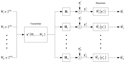
Figure 2: A Gaussian vector broadcast channel.

For clarity, we use $\mathbf{\Gamma}_{i}$ to specifically denote the input covariance matrix of link $i$ in a MIMO-BC, and $\mathbf{Q}_{j}$ to denote an input covariance matrix in other types of MIMO channels. From the encoding process of DPC, the achievable rate in DPC scheme can be computed as follows:

$$R_{\pi(i)}=\log\frac{\left|\mathbf{I}+\mathbf{H}_{\pi(i)}\left(\sum_{j\geq i}\mathbf{\Gamma}_{\pi(j)}\right)\mathbf{H}_{\pi(i)}^{{\dagger}}\right|}{\left|\mathbf{I}+\mathbf{H}_{\pi(i)}\left(\sum_{j>i}\mathbf{\Gamma}_{\pi(j)}\right)\mathbf{H}_{\pi(i)}^{{\dagger}}\right|},$$ (8)

where $\pi$ denotes a permutation of the set $\{1,\ldots,K\}$, $\pi(i)$ represents the $i^{th}$ position in permutation $\pi$. One important observation of the dirty paper rate equation in (8) is that the rate equation is neither a concave nor a convex function of the input covariance matrices $\mathbf{\Gamma}_{i}$, $i=1,2,\ldots,K$.

Let $\mathbf{H}=[\mathbf{H}_{1},\ldots,\mathbf{H}_{K}]^{T}$ be the collection of $K$ channel gain matrices in the MIMO-BC, and $\mathbf{\Gamma}=[\mathbf{\Gamma}_{1}\,\ldots,\mathbf{\Gamma}_{K}]$ be the collection of $K$ input covariance matrices. We define the dirty paper region $\mathcal{C}_{DPC}(P,\mathbf{H})$ as the convex hull of the union of all such rates vectors over all positive semidefinite covariance matrices $\mathbf{\Gamma}_{1},\ldots,\mathbf{\Gamma}_{K}$ satisfying $\mathrm{Tr}\{\sum_{i=1}^{K}\mathbf{\Gamma}_{i}\}\leq P$ (the maximum transmit power constraint at the transmitter) and over all $K!$ permutations:

$$\mathcal{C}_{\mathrm{DPC}}(P,\mathbf{H})\triangleq Cov\left(\cup_{\pi,\mathbf{\Gamma}}\mathbf{R}^{\mathrm{BC}}(\pi,\mathbf{\Gamma})\right),$$

where $Cov(\cdot)$ represents the convex hull operation.

II-D Problem Formulation

In this paper, we aim to solve the problem of jointly optimizing DPC per-antenna power allocation at each node in the link layer and multihop/multipath routing in a MIMO-based WMN. Suppose that each node in the network has been assigned a certain (possibly reused) frequency band that will not cause interference to any other node in the network. Also, the incoming and outgoing bands of each node are non-overlapping such that each node can transmit and receive simultaneously. How to perform channel assignments is a huge research topic on its own merits, and there are a vast amount of literature that discuss channel assignment problems. Thus, in this paper, we focus on how to jointly optimize routing in the network layer and the DPC power allocation in the link layer for each node when a channel assignment is given. We adopt the well-known proportional fairness utility function, i.e., $\ln(s_{f})$ for flow $f$. In CRPA, we wish to maximize the sum of all utility functions. In the link layer, since the total transmit power of each node is subject to a maximum power constraint, we have $\sum_{l\in\mathcal{O}\left(n\right)}\mathrm{Tr}\{\mathbf{\Gamma}_{l}\}\leq P_{\max}^{(n)}$, $1\leq n\leq N$, where $P_{\max}^{(n)}$ represents the maximum transmit power of node $n$. Since the total amount of flow in each link $l$ cannot exceed its capacity limit, we must have $\sum_{f=1}^{F}t_{l}^{(f)}\leq R_{l}(\mathbf{\Gamma})$, $1\leq l\leq L$. This can be further compactly written using matrix-vector notations as $\langle\mathbf{1},\mathbf{T}^{T}\mathbf{e}_{l}\rangle\leq R_{l}(\mathbf{\Gamma})$, $1\leq l\leq L$. Coupling the network layer model in Section II-A and MIMO-BC link layer model in Section II-C, we have the problem formulation for CRPA as in (9).

$$\begin{array}[]{rll}\mbox{\text@underline{{CRPA:}}}&&\\ \mbox{Maximize}&\sum_{f=1}^{F}\ln(s_{f})&\\ \mbox{subject to}&\mathbf{A}\mathbf{T}=\mathbf{S}&\\ &\mathbf{T}\geq\mathbf{0}&\\ &\mathbf{S}\mathbf{e}_{f}=_{\mathrm{src}(f),\mathrm{dst}(f)}\mathbf{0}&\!\!\!\forall\,f\\ &\langle\mathbf{1},\mathbf{S}\mathbf{e}_{f}\rangle=0&\!\!\!\forall\,f\\ &(\mathbf{S}\mathbf{e}_{f})_{\mathrm{src}(f)}=s_{f}&\!\!\!\forall\,f\\ &\langle\mathbf{1},\mathbf{T}^{T}\mathbf{e}_{l}\rangle\leq R_{l}(\mathbf{\Gamma})&\!\!\!\forall\,l\\ &R_{l}(\mathbf{\Gamma})\in\mathcal{C}_{\mathrm{DPC}}^{(n)}(P_{\max}^{(n)},\mathbf{H}^{(n)})&\!\!\!\forall l\in\mathcal{O}\left(n\right)\\ &\sum_{l\in\mathcal{O}\left(n\right)}\mathrm{Tr}\{\mathbf{\Gamma}_{l}\}\leq P_{\max}^{(n)}&\!\!\!\forall\,n\\ &\mathbf{\Gamma}_{l}\succeq 0&\!\!\!\forall\,l\\ &\mbox{Variables: }\mathbf{S},\,\mathbf{T},\,\mathbf{\Gamma}&\\ \end{array}$$ (9)

III Reformulation of CRPA

As we pointed out earlier, the DPC rate equation in (8) is neither a concave nor a convex function of the input covariance matrices. As a result, the cross-layer optimization problem in (9) is a non-convex optimization problem, which is very hard to solve numerically, let alone analytically. However, in the following, we will show that (9) can be reformulated as an equivalent convex optimization problem by projecting all the MIMO-BC channels onto their dual MIMO multiple-access channels (MIMO-MAC). We first provide some background of Gaussian vector multiple access channels and the channel duality between MIMO-BC and MIMO-MAC.

III-A MIMO-MAC Channel Model

A communication system where multiple uncoordinated transmitters send independent information to a single receiver is referred to as a multiple access channel. If the channel gain of each link in the multiple access channel is a matrix and the noise is a Gaussian random vector, the channel is termed “Gaussian vector multiple access channel”. Fig. 3 illustrates a $K$-user Gaussian vector multiple access channel, where independent messages $W_{1},\ldots,W_{K}$, are encoded by transmitters 1 to $K$, respectively, and the receiver is trying to decode $W_{1},\ldots,W_{K}$. A $(n,2^{nR_{1}},\ldots,2^{nR_{K}})_{\mathrm{MAC}}$ codebook for a multiple access channel consists of encoding functions $\mathbf{x}_{1}^{n}(W_{1}),\ldots,\mathbf{x}_{K}^{n}(W_{K})$ where $W_{i}\in\{1,\ldots,2^{nR_{i}}\}$, $i=1,2,\ldots,K$. The decoding functions at the receiver are $\hat{W}_{i}(\mathbf{y}_{i}^{n})$, $i=1,2,\ldots,K$. An error occurs when $\hat{W}_{i}\neq W_{i}$. A rate vector $\mathbf{R}=[R_{1},\ldots,R_{K}]^{T}$ is said to be achievable if there exists a sequence of $(n,2^{nR_{1}},\ldots,2^{nR_{K}})_{\mathrm{MAC}}$ codebooks for which the average probability of error $P_{e}\rightarrow 0$ as the code length $n\rightarrow\infty$. The capacity region of a multiple access channel, denoted by $\mathcal{C}_{\mathrm{MAC}}$ is defined as the union of all achievable rate vectors [3]. We call the Gaussian vector multiple access channel in the MIMO case as MIMO-MAC throughout the rest of this paper.

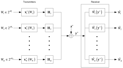
Figure 3: A Gaussian vector multiple access channel.

III-B Duality between MIMO-BC and MIMO-MAC

The dual MIMO-MAC of a MIMO-BC can be constructed by changing the receivers in the MIMO-BC into transmitters and changing the transmitter in the MIMO-BC into the receiver. The channel gain matrices in dual MIMO-MAC are the conjugate transpose of the channel gain matrices in MIMO-BC. The maximum sum power in the dual MIMO-MAC is the same maximum power level as in MIMO-BC. The relationship between a MIMO-BC and its dual MIMO-MAC is illustrated in Fig. 4. Similar to MIMO-BC, We denote the capacity region of the dual MIMO-MAC as $\mathcal{C}_{\mathrm{MAC}}(P,\mathbf{H}^{{\dagger}})$.

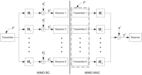
Figure 4: The relationship between MIMO-BC and its dual MIMO-MAC

The following Lemma states the relationship between the capacity regions of a MIMO-BC and its dual MIMO-MAC.

Lemma 1

The DPC region of a MIMO-BC channel with maximum power constraint $P$ is equal to the capacity region of the dual MIMO MAC with sum power constraint $P$

$$\mathcal{C}_{\mathrm{DPC}}(P,\mathbf{H})=\mathcal{C}_{\mathrm{MAC}}(P,\mathbf{H}^{{\dagger}}).$$

Proof:

The proof of this theorem can be arrived in various ways [8, 9, 10]. The most straightforward approach is to show that any MIMO-BC achievable rate vector is also achievable in its dual MIMO-MAC and vice versa. The MAC-to-BC and BC-to-MAC mappings can be found in [8]. It is also shown in [8] that any rate vector in a MIMO-BC with a particular encoding order can be achieved in its dual MIMO-MAC with the reversed successive decoding order. ∎

III-C Convexity of MIMO-MAC Capacity Region

From Lemma 1, we know that the capacity region of a MIMO-BC and its dual MIMO-MAC is exactly the same. Therefore, we can replace $\mathcal{C}_{\mathrm{DPC}}(\cdot)$ in (9) by the capacity regions of the dual MIMO-MAC channels $\mathcal{C}_{\mathrm{MAC}}(\cdot)$. The benefits of such replacements is due to the following theorem.

Theorem 1

The capacity region of a $K$-user MIMO-MAC channel with a sum power constraint $\sum_{i=1}^{K}\mathrm{Tr}(\mathbf{Q}_{i})\leq P_{\max}$ is convex with respect to the input covariance matrices $\mathbf{Q}_{1},\ldots,\mathbf{Q}_{K}$.

Proof:

Denote the input signals of the $K$ users by $\mathbf{x}_{1},\ldots,\mathbf{x}_{K}$, respectively, and denote the output of the MIMO-MAC channel by $\mathbf{y}$. Since $\rho_{i}$ is a scalar, we absorb $\rho_{i}$ into $\mathbf{H}_{i}$ in this proof for notation convenience. Theorem 14.3.5 in [3] states that the capacity region of a MIMO-MAC is determined by

$$\mathcal{C}_{\mathrm{MAC}}(\mathbf{Q}_{1},\ldots,\mathbf{Q}_{K})=$$ (14)

$$Cov\left\{(R_{1},\ldots,R_{K})\left|\begin{array}[]{l}\sum_{i\in\mathcal{S}}R_{i}(\mathbf{Q})\leq\\ I(\mathbf{x}_{i},i\in\mathcal{S};\mathbf{y}|\mathbf{x}_{i},{i\in\mathcal{S}^{c}}),\\ \forall\mathcal{S}\subseteq\{1,\ldots,K\}\\ \sum_{i=1}^{K}\mathrm{Tr}(\mathbf{Q}_{i})\leq P_{\max}\end{array}\right.\right\},$$

where the mutual information expression $I(;)$ can be bounded as follows:

$$I(\mathbf{x}_{i},{i\in\mathcal{S}};\mathbf{y}|\mathbf{x}_{i},{i\in\mathcal{S}^{c}})\leq\log\left|\mathbf{I}+\sum_{i\in\mathcal{S}}\mathbf{H}_{i}^{{\dagger}}\mathbf{Q}_{i}\mathbf{H}_{i}\right|.$$ (15)

To show that the capacity region of the MIMO-MAC with a sum power constraint is convex, it is equivalent to show that the convex hull operation in (14) is unnecessary. To show this, consider the convex combination of two arbitrarily chosen achievable rate vectors $[R_{1},\ldots,R_{K}]$ and $[\hat{R}_{1},\ldots,\hat{R}_{K}]$ determined by two feasible power vectors $[\mathbf{Q}_{1},\ldots,\mathbf{Q}_{K}]$ and $[\hat{\mathbf{Q}}_{1},\ldots,\hat{\mathbf{Q}}_{K}]$, respectively, i.e., we have $\sum_{i=1}^{K}\mathrm{Tr}(\mathbf{Q}_{i})\leq P_{\max}$ and $\sum_{i=1}^{K}\mathrm{Tr}(\hat{\mathbf{Q}}_{i})\leq P_{\max}$. Let $0\leq\alpha\leq 1$ and consider the convex combination

$$[\bar{R}_{1},\ldots,\bar{R}_{K}]=\alpha[R_{1},\ldots,R_{K}]+(1-\alpha)[\hat{R}_{1},\ldots,\hat{R}_{K}].$$

Also, let $\bar{\mathbf{Q}}_{i}=\alpha\mathbf{Q}_{i}+(1-\alpha)\hat{\mathbf{Q}}_{i}$, $i=1,\ldots,K$. It is easy to verify that $\sum_{i=1}^{K}\mathrm{Tr}(\bar{\mathbf{Q}}_{i})\leq P_{\max}$, i.e., the convex combination of two feasible power vectors is also feasible. Now, consider

$$\alpha\sum_{i\in\mathcal{S}}R_{i}+(1-\alpha)\sum_{i\in\mathcal{S}}\hat{R}_{i}\leq\alpha\log\left|\mathbf{I}+\sum_{i\in\mathcal{S}}\mathbf{H}_{i}^{{\dagger}}\mathbf{Q}_{i}\mathbf{H}_{i}\right|$$

$$+(1-\alpha)\log\left|\mathbf{I}+\sum_{i\in\mathcal{S}}\mathbf{H}_{i}^{{\dagger}}\hat{\mathbf{Q}}_{i}\mathbf{H}_{i}\right|.$$

Since the function $\log|\mathbf{A}|$ is a concave function for any positive semidefinite matrix variable $\mathbf{A}$ [3], it follows from Jensen’s inequality that

$$\alpha\sum_{i\in\mathcal{S}}R_{i}+(1-\alpha)\sum_{i\in\mathcal{S}}\hat{R}_{i}\leq\frac{1}{2}\log\left|\mathbf{I}+\sum_{i\in\mathcal{S}}\mathbf{H}_{i}^{{\dagger}}\bar{\mathbf{Q}}_{i}\mathbf{H}_{i}\right|,$$

which means that the convex combination of rate vectors $[R_{1},\ldots,R_{K}]$ and $[\hat{R}_{1},\ldots,\hat{R}_{K}]$ can also be achieved by using the feasible power vector $[\bar{\mathbf{Q}}_{1},\ldots,\bar{\mathbf{Q}}_{K}]$ directly. As a result, the convex hull operation is unnecessary. ∎

III-D Maximum Weighted Sum Rate Problem of the Dual MIMO-MAC

Now, we consider the maximum weighted sum rate problem of the dual MIMO-MAC. We simplify this problem such that we do not have to enumerate all possible successive decoding order in the dual MIMO-MAC, thus paving the way to efficiently solve the link layer subproblem we discuss in Section IV.

Theorem 2

Associate each rate $R_{i}$ in MIMO-MAC a non-negative weight $u_{i}$, $i=1,\ldots,K$, the maximum weighted sum $\max\sum_{i=1}^{K}R_{i}(\mathbf{Q})$ can be solved by the following convex optimization problem:

$$\begin{array}[]{rl}\!\!\!\!\!\!\mbox{Maximize}&\!\!\!\sum_{i=1}^{K}(u_{\pi(i)}-u_{\pi(i-1)})\times\\ \!\!\!\!\!\!&\!\!\!\log\left|\mathbf{I}+\sum_{j=i}^{K}\rho_{\pi(j)}\mathbf{H}_{\pi(j)}^{{\dagger}}\mathbf{Q}_{\pi(j)}\mathbf{H}_{\pi(j)}\right|\\ \!\!\!\!\!\!\mbox{subject to}&\!\!\!\sum_{i=1}^{K}\mathrm{Tr}(\mathbf{Q}_{i})\leq P_{\max}\\ \!\!\!\!\!\!&\!\!\!\mathbf{Q}_{i}\succeq 0,\,\,i=1,\ldots,K,\end{array}$$ (16)

where $u_{\pi(0)}\triangleq 0$, $\pi(i),i=1,\ldots,K$ is a permutation on $\{1,\ldots,K\}$ such that $u_{\pi(1)}\leq\ldots\leq u_{\pi(K)}$. In particular, suppose that $(\mathbf{Q}_{\pi(1)}^{*},\ldots,\mathbf{Q}_{\pi(K)}^{*})$ solves (16), then the optimal rates of (16) are given by

$$R_{\pi(K)}^{*}=\log\left|\mathbf{I}+\rho_{\pi(K)}\mathbf{H}_{\pi(K)}^{{\dagger}}\mathbf{Q}_{\pi(K)}^{*}\mathbf{H}_{K}\right|$$ (17)

and

$$R_{\pi(i)}^{*}=\log\left|\mathbf{I}+\sum_{j=i}^{K}\rho_{\pi(j)}\mathbf{H}_{\pi(j)}^{{\dagger}}\mathbf{Q}_{\pi(j)}^{*}\mathbf{H}_{j}\right|$$

$$\quad\quad-\log\left|\mathbf{I}+\sum_{j=i+1}^{K}\rho_{\pi(j)}\mathbf{H}_{\pi(j)}^{{\dagger}}\mathbf{Q}_{\pi(j)}^{*}\mathbf{H}_{j}\right|,$$ (18)

for $i=1,2,\ldots,K-1$.

Proof:

For convenience, we let

$$\Phi(\mathcal{S})=\log\left|\mathbf{I}+\sum_{i\in\mathcal{S}}\mathbf{H}_{\pi(i)}^{{\dagger}}\mathbf{Q}_{\pi(i)}\mathbf{H}_{\pi(i)}\right|.$$

Since $\pi(i)$ is simply a permutation on $\{1,\ldots,K\}$, from (14) and (15) we have the maximum weighted sum rate problem can be written as

$$\begin{array}[]{rl}\mbox{Maximize}&\sum_{i=1}^{K}u_{\pi(i)}R_{\pi(i)}\\ \mbox{subject to}&\sum_{i\in\mathcal{S}}R_{\pi(i)}\leq\Phi(\mathcal{S}),\,\,\forall\mathcal{S}\subseteq\{1,\ldots,K\}.\end{array}$$

Also from (14) and (15), it is easy to derive that $R_{\pi(i)}\leq\Phi(\{\pi(i)\})=\log\left|\mathbf{I}+\rho_{\pi(i)}\mathbf{H}_{\pi(i)}^{{\dagger}}\mathbf{Q}_{\pi(i)}\mathbf{H}_{\pi(i)}\right|$. Since $u_{\pi(1)}\leq\ldots\leq u_{\pi(K)}$, from KKT condition, we must have that the constraint $R_{\pi(K)}=\Phi(\{\pi(K)\})$ must be tight at optimality. That is,

$$R_{\pi(K)}=\log\left|\mathbf{I}+\rho_{\pi(K)}\mathbf{H}_{\pi(K)}^{{\dagger}}\mathbf{Q}_{\pi(K)}\mathbf{H}_{\pi(K)}\right|.$$ (19)

Again, from (14) and (15), we have

$$R_{\pi(K-1)}+R_{\pi(K)}\leq\log\left|\mathbf{I}+\rho_{\pi(K)}\mathbf{H}_{\pi(K)}^{{\dagger}}\mathbf{Q}_{\pi(K)}\mathbf{H}_{\pi(K)}\right.$$

$$\left.+\rho_{\pi(K-1)}\mathbf{H}_{\pi(K-1)}^{{\dagger}}\mathbf{Q}_{\pi(K-1)}\mathbf{H}_{\pi(K-1)}\right|.$$

So,

$$R_{\pi(K-1)}\leq\log\left|\mathbf{I}+\rho_{\pi(K)}\mathbf{H}_{\pi(K)}\mathbf{Q}_{\pi(K)}\mathbf{H}_{\pi(K)}^{{\dagger}}\right.$$

$$\left.+\rho_{\pi(K-1)}\mathbf{H}_{\pi(K-1)}\mathbf{Q}_{\pi(K-1)}\mathbf{H}_{\pi(K-1)}^{{\dagger}}\right|-$$

$$\log\left|\mathbf{I}+\rho_{\pi(K)}\mathbf{H}_{\pi(K)}\mathbf{Q}_{\pi(K)}\mathbf{H}_{\pi(K)}^{{\dagger}}\right|$$ (20)

Since $u_{\pi(K-1)}$ is the second largest weight, again from KKT condition, we must have that (III-D) must be tight at optimality. This process continues for all $K$ users. Subsequently, we have that

$$R_{\pi(i)}=\log\left|\mathbf{I}+\sum_{j=i}^{K}\rho_{\pi(j)}\mathbf{H}_{\pi(j)}^{{\dagger}}\mathbf{Q}_{\pi(j)}\mathbf{H}_{j}\right|$$

$$\quad\quad-\log\left|\mathbf{I}+\sum_{j=i+1}^{K}\rho_{\pi(j)}\mathbf{H}_{\pi(j)}^{{\dagger}}\mathbf{Q}_{\pi(j)}\mathbf{H}_{j}\right|,$$ (21)

for $i=1,\ldots,K-1$. Summing up all $u_{\pi(i)}R_{\pi(i)}$ and after rearranging the terms, it is readily verifiable that

$$\sum_{i=1}^{K}u_{\pi(i)}R_{\pi(i)}=\sum_{i=1}^{K}(u_{\pi(i)}-u_{\pi(i-1)})\times$$

$$\log\left|\mathbf{I}+\sum_{j=i}^{K}\rho_{\pi(j)}\mathbf{H}_{\pi(j)}^{{\dagger}}\mathbf{Q}_{\pi(j)}\mathbf{H}_{\pi(j)}\right|.$$ (22)

It then follows that the maximum weighted sum rate problem of MIMO-MAC is equivalent to maximizing (III-D) subject to the sum power constraint, i.e., the optimization problem in (16). Since $\log\left|\cdot\right|$ is a concave function of positive semidefinite matrices, (III-D) is a convex optimization problem with respect to $\mathbf{Q}_{\pi(1)},\ldots,\mathbf{Q}_{\pi(K)}$. After we obtain the optimal solution power solution $(\mathbf{Q}_{\pi(1)}^{*},\ldots,\mathbf{Q}_{\pi(K)}^{*})$, the corresponding link rates can be computed by simply following (19) and (III-D). ∎

III-E Problem Reformulation

We now reformulate CRPA by replacing $\mathcal{C}_{\mathrm{DPC}}$ in (9) with $\mathcal{C}_{\mathrm{MAC}}$, and we denote the equivalent problem by CRPA-E. After solving CRPA-E, we can recover the corresponding MIMO-BC covariance matrices $\mathbf{\Gamma}^{*}$ from the optimal solution $\mathbf{Q}^{*}$ of CRPA-E by the MAC-to-BC mapping provided in [8].

$$\begin{array}[]{rll}\mbox{\text@underline{{CRPA-E:}}}&&\\ \mbox{Maximize}&\sum_{f=1}^{F}\ln(s_{f})&\\ \mbox{subject to}&\mathbf{A}\mathbf{T}=\mathbf{S}&\\ &\mathbf{T}\geq\mathbf{0}&\\ &\mathbf{S}\mathbf{e}_{f}=_{\mathrm{src}(f),\mathrm{dst}(f)}\mathbf{0}&\!\!\!\forall\,f\\ &\langle\mathbf{1},\mathbf{S}\mathbf{e}_{f}\rangle=0&\!\!\!\forall\,f\\ &(\mathbf{S}\mathbf{e}_{f})_{\mathrm{src}(f)}=s_{f}&\!\!\!\forall\,f\\ &\langle\mathbf{1},\mathbf{T}^{T}\mathbf{e}_{l}\rangle\leq R_{l}(\mathbf{Q})&\!\!\!\forall\,l\\ &R_{l}(\mathbf{Q})\in\mathcal{C}_{\mathrm{MAC}}^{(n)}(P_{\max}^{(n)},\mathbf{H}^{{\dagger}(n)})&\!\!\!\forall l\in\mathcal{O}\left(n\right)\\ &\sum_{l\in\mathcal{O}\left(n\right)}\mathrm{Tr}\{\mathbf{Q}_{l}\}\leq P_{\max}^{(n)}&\!\!\!\forall\,n\\ &\mathbf{Q}_{l}\succeq 0&\!\!\!\forall\,l\\ &\mbox{Variables: }\mathbf{S},\,\mathbf{T},\,\mathbf{Q}&\\ \end{array}$$ (23)

IV Solution Procedure

Since CRPA-E is a convex programming problem, we can solve CRPA-E exactly by solving its Lagrangian dual problem. Introducing Lagrangian multipliers $u_{i}$ to the link capacity coupling constraints $\langle\mathbf{1},\mathbf{T}^{T}\mathbf{e}_{l}\rangle\leq R_{l}(\mathbf{Q})$, Hence, we can write the Lagrangian as

$$\Theta(\mathbf{u})=\sup_{\mathbf{S},\mathbf{T},\mathbf{Q}}\left\{L(\mathbf{S},\mathbf{T},\mathbf{Q},\mathbf{u})|(\mathbf{S},\mathbf{T},\mathbf{Q})\in\Psi\right\},$$ (24)

where

$$L(\mathbf{S},\mathbf{T},\mathbf{Q},\mathbf{u})=\sum_{f}\ln\left(s_{f}\right)+\sum_{l}u_{l}\left(R_{l}(\mathbf{Q})-\langle\mathbf{1},\mathbf{T}^{T}\mathbf{e}_{l}\rangle\right)$$

and $\Psi$ is defined as

$${\small\Psi\triangleq\left\{(\mathbf{S},\mathbf{T},\mathbf{Q})\left|\begin{array}[]{ll}\mathbf{A}\mathbf{T}=\mathbf{S}\\ \mathbf{T}\geq\mathbf{0}\\ \mathbf{S}\mathbf{e}_{f}=_{\mathrm{src}(f),\mathrm{dst}(f)}\mathbf{0}&\forall\,f\\ \langle\mathbf{1},\mathbf{S}\mathbf{e}_{f}\rangle=0&\forall\,f\\ (\mathbf{S}\mathbf{e}_{f})_{\mathrm{src}(f)}=s_{f}&\forall\,f\\ \sum_{l\in\mathcal{O}\left(n\right)}\mathrm{Tr}\{\mathbf{Q}_{l}\}\leq P_{\max}^{(n)}&\forall\,n\\ \mathbf{Q}_{l}\succeq 0&\forall\,l\\ R_{l}(\mathbf{Q})\in\mathcal{C}_{\mathrm{MAC}}(P_{\max}^{(n)},\mathbf{H}^{{\dagger}(n)})&\forall\,n\\ \end{array}\right.\right\}}.$$

The Lagrangian dual problem of CRPA can thus be written as:

$$\begin{array}[]{rll}\mathbf{D}^{\mathrm{CRPA-E}}:\quad\mbox{Minimize}&\Theta(\mathbf{u})&\\ \mbox{subject to}&\mathbf{u}\geq\mathbf{0}.\\ \end{array}$$

It is easy to recognize that, for a given $\mathbf{u}$, the Lagrangian in (24) can be rearranged and separated into two terms:

$$\Theta(\mathbf{u})=\Theta_{\mathrm{net}}(\mathbf{u})+\Theta_{\mathrm{link}}(\mathbf{u}),$$

where, for a given Lagrangian multiplier $\mathbf{u}$, $\Theta_{\mathrm{net}}$ and $\Theta_{\mathrm{link}}$ are corresponding to network layer and link layer variables, respectively:

$$\begin{array}[]{rll}\mathbf{D}^{\mathrm{CRPA-E}}_{\mathrm{net}}:\Theta_{\mathrm{net}}(\mathbf{u})\triangleq&\mbox{Maximize}\sum_{f}\ln\left(s_{f}\right)\\ &\quad-\sum_{l}u_{l}\langle\mathbf{1},\mathbf{T}^{T}\mathbf{e}_{l}\rangle&\\ \mbox{subject to}&\mathbf{A}\mathbf{T}=\mathbf{S}&\\ &\mathbf{T}\geq\mathbf{0}&\\ &\mathbf{S}\mathbf{e}_{f}=_{\mathrm{src}(f),\mathrm{dst}(f)}\mathbf{0}&\forall\,f\\ &\langle\mathbf{1},\mathbf{S}\mathbf{e}_{f}\rangle=0&\forall\,f\\ &(\mathbf{S}\mathbf{e}_{f})_{\mathrm{src}(f)}=s_{f}&\forall\,f\\ \mbox{Variables: }&\mathbf{S},\,\mathbf{T}&\end{array}$$

$$\begin{array}[]{rll}\mathbf{D}^{\mathrm{CRPA-E}}_{\mathrm{link}}:\Theta_{\mathrm{link}}(\mathbf{u})\triangleq&\mbox{Maximize}\sum_{l}u_{l}R_{l}(\mathbf{Q})&\\ \mbox{subject to}&\sum_{l\in\mathcal{O}\left(n\right)}\mathrm{Tr}\{\mathbf{Q}_{l}\}\leq P_{\max}^{(n)}&\forall\,n\\ &\mathbf{Q}_{l}\succeq 0&\forall\,l\\ &R_{l}(\mathbf{Q})\in\mathcal{C}_{\mathrm{MAC}}(P_{\max}^{(n)},\mathbf{H}^{{\dagger}(n)}),&\\ &\quad\quad\forall\,l\in\mathcal{O}\left(n\right),n\in N&\\ \mbox{Variables: }&\mathbf{Q}&\end{array}$$

The CRPA-E Lagrangian dual problem can thus be written as the following master dual problem:

$$\begin{array}[]{rll}\mathbf{MD}^{\mathrm{CRPA-E}}:\quad\mbox{Minimize}&\Theta_{\mathrm{net}}(\mathbf{u})+\Theta_{\mathrm{link}}(\mathbf{u})&\\ \mbox{subject to}&\mathbf{u}\geq\mathbf{0}\\ \end{array}$$

Notice that $\Theta_{\mathrm{link}}(\mathbf{u})$ can be further decomposed on a node-by-node basis as follows:

$$\Theta_{\mathrm{link}}(\mathbf{u})=\max\sum_{l}u_{l}R_{l}(\mathbf{Q})$$

$$=\sum_{n=1}^{N}\left(\max\sum_{l\in\mathcal{O}\left(n\right)}u_{l}R_{l}(\mathbf{Q})\right)=\sum_{n=1}^{N}\Theta_{\mathrm{link}}^{(n)}(\mathbf{u}^{(n)}).$$ (27)

It is seen that $\Theta_{\mathrm{link}}^{(n)}(\mathbf{u}^{(n)})\triangleq\max\sum_{l\in\mathcal{O}\left(n\right)}u_{l}R_{l}(\mathbf{Q})$ is a maximum weighted sum rate problem of the dual MIMO-MAC for some given dual variables $\mathbf{u}^{(n)}$ as weights. Without loss of generality, suppose that node $n$ has $K$ outgoing links, which are indexed as $1,\ldots,K$ and are associated with dual variables $u_{1},\ldots,u_{K}$, respectively. Let $\pi(i)\in\{1,\ldots,K\}$ be the permutation such that $0\leq u_{\pi(1)}\leq\ldots\leq u_{\pi(K)}$ and define $u_{\pi(0)}=0$. $\Theta_{\mathrm{link}}^{(n)}(\mathbf{u}^{(n)})$ can be written as follows:

$$\begin{array}[]{rl}\mbox{Maximize}&\!\!\!\sum_{i=1}^{K}(u_{\pi(i)}-u_{\pi(i-1)})\times\\ &\!\!\!\log\left|\mathbf{I}+\sum_{j=i}^{K}\rho_{\pi(j)}\mathbf{H}_{\pi(j)}^{{\dagger}}\mathbf{Q}_{\pi(j)}\mathbf{H}_{\pi(j)}\right|\\ \mbox{subject to}&\!\!\!\sum_{i=1}^{K}\mathrm{Tr}(\mathbf{Q}_{i})\leq P_{\max}^{(n)}\\ &\!\!\!\mathbf{Q}_{i}\succeq 0,\,\,i=1,\ldots,K.\end{array}$$ (28)

Note that in the network layer subproblem $\Theta_{\mathrm{net}}(\mathbf{u})$, the objective function is concave and all constraints are affine. Therefore, $\Theta_{\mathrm{net}}(\mathbf{u})$ is readily solvable by many polynomial time convex programming methods. However, even though $\Theta_{\mathrm{link}}^{(n)}(\mathbf{u}^{(n)})$ is also a convex problem, generic convex programming methods are not efficient because the structures of its objective function and constraints are very complex. In the following subsections, we will discuss in detail how to solve $\Theta_{\mathrm{link}}^{(n)}(\mathbf{u}^{(n)})$.

IV-A Conjugate Gradient Projection for Solving $\Theta_{\mathrm{link}}^{(n)}(\mathbf{u}^{(n)})$

We propose an efficient algorithm based on conjugate gradient projection (CGP) to solve (28). CGP utilizes the important and powerful concept of Hessian conjugacy to deflect the gradient direction appropriately so as to achieve the superlinear convergence rate [11], which is similar to that of the well-known quasi-Newton methods (e.g., BFGS method). In each iteration, CGP projects the conjugate gradient direction to find an improving feasible direction. The framework of CGP for solving (28) is shown in Algorithm 1.

Algorithm 1 Gradient Projection Method

  Initialization:

   Choose the initial conditions $\mathbf{Q}^{(0)}=[\mathbf{Q}_{1}^{(0)},\mathbf{Q}_{2}^{(0)},\ldots,\mathbf{Q}_{K}^{(0)}]^{T}$. Let

   $k=0$.

  Main Loop:

   1. Calculate the conjugate gradients $\mathbf{G}_{i}^{(k)}$, $i=1,2,\ldots,K$.

   2. Choose an appropriate step size $s_{k}$. Let $\mathbf{Q}_{i}^{{}^{\prime}(k)}=\mathbf{Q}_{i}^{(k)}+s_{k}\mathbf{G}_{i}^{(k)}$,

    for $i=1,2,\ldots,K$.

   3. Let $\bar{\mathbf{Q}}^{(k)}$ be the projection of $\mathbf{Q}^{{}^{\prime}(k)}$ onto $\Omega_{+}(P_{\max}^{(n)})$.

   4. Choose an appropriate step size $\alpha_{k}$. Let $\mathbf{Q}_{l}^{(k+1)}=\mathbf{Q}_{l}^{(k)}+$

    $\alpha_{k}(\bar{\mathbf{Q}}_{i}^{(k)}-\mathbf{Q}_{i}^{(k)})$, $i=1,2,\ldots,K$.

   5. $k=k+1$. If the maximum absolute value of the elements in $\mathbf{Q}_{i}^{(k)}-$

    $\mathbf{Q}_{i}^{(k-1)}<\epsilon$, for $i=1,2,\ldots,L$, then stop; else go to step 1.

We adopt the “Armijo’s Rule” inexact line search method to avoid excessive objective function evaluations, while still enjoying provable convergence [11]. For convenience, we use $F(\mathbf{Q})$ to represent the objective function in (28), where $\mathbf{Q}=(\mathbf{Q}_{1},\ldots,\mathbf{Q}_{K})$ denotes the set of covariance matrices at a node. According to Armijo’s Rule, in the $k^{th}$ iteration, we choose $\sigma_{k}=1$ and $\alpha_{k}=\beta^{m_{k}}$ (the same as in [12]), where $m_{k}$ is the first non-negative integer $m$ that satisfies

$$F(\mathbf{Q}^{(k+1)})-F(\mathbf{Q}^{(k)})\geq\sigma\beta^{m}\langle\mathbf{G}^{(k)},\bar{\mathbf{Q}}^{(k)}-\mathbf{Q}^{(k)}\rangle$$

$$=\sigma\beta^{m}\sum_{i=1}^{K}\mathrm{Tr}\left[\mathbf{G}_{i}^{{\dagger}(k)}\left(\bar{\mathbf{Q}}_{i}^{(k)}-\mathbf{Q}_{i}^{(k)}\right)\right],$$ (29)

where $0<\beta<1$ and $0<\sigma<1$ are fixed scalars.

IV-B Computing the Conjugate Gradients

The gradient $\bar{\mathbf{G}}_{\pi(j)}\triangleq\nabla_{\mathbf{Q}_{\pi(j)}}F(\mathbf{Q})$ depends on the partial derivatives of $F(\mathbf{Q})$ with respect to $\mathbf{Q}_{\pi(j)}$. By using the formula $\frac{\partial\ln\left|\mathbf{A}+\mathbf{B}\mathbf{X}\mathbf{C}\right|}{\partial\mathbf{X}}=\left[\mathbf{C}(\mathbf{A}+\mathbf{B}\mathbf{X}\mathbf{C})^{-1}\mathbf{B}\right]^{T}$ [12, 13], we can compute the partial derivative of the $i^{th}$ term in the summation of $F(\mathbf{Q})$ with respect to $\mathbf{Q}_{\pi(j)}$, $j\geq i$, as follows:

$$\frac{\partial}{\partial\mathbf{Q}_{\pi(j)}}\Bigg{(}(u_{\pi(i)}-u_{\pi(i-1)})\times$$

$$\hskip 21.68121pt\left.\log\left|\mathbf{I}+\sum_{k=i}^{K}\rho_{\pi(k)}\mathbf{H}_{\pi(k)}^{{\dagger}}\mathbf{Q}_{\pi(k)}\mathbf{H}_{\pi(k)}\right|\right)$$

$$=\rho_{\pi(j)}\left(u_{\pi(i)}-u_{\pi(i-1)}\right)\times$$

$$\left[\mathbf{H}_{\pi(j)}\left(\mathbf{I}+\sum_{k=i}^{K}\rho_{\pi(k)}\mathbf{H}_{\pi(k)}^{{\dagger}}\mathbf{Q}_{\pi(k)}\mathbf{H}_{\pi(k)}\right)^{-1}\mathbf{H}_{\pi(j)}^{{\dagger}}\right]^{T}.$$

To compute the gradient of $F(\mathbf{Q})$ with respect to $\mathbf{Q}_{\pi(j)}$, we notice that only the first $j$ terms in $F(\mathbf{Q})$ involve $\mathbf{Q}_{\pi(j)}$. From the definition $\nabla_{z}f(z)=2(\partial f(z)/\partial z)^{*}$ [14], we have

$$\bar{\mathbf{G}}_{\pi(j)}=2\rho_{\pi(j)}\mathbf{H}_{\pi(j)}\Bigg{[}\sum_{i=1}^{j}\left(u_{\pi(i)}-u_{\pi(i-1)}\right)\times$$

$$\left.\left(\mathbf{I}+\sum_{k=i}^{K}\rho_{\pi(k)}\mathbf{H}_{\pi(k)}^{{\dagger}}\mathbf{Q}_{\pi(k)}\mathbf{H}_{\pi(k)}\right)^{-1}\right]\mathbf{H}_{\pi(j)}^{{\dagger}}.$$ (30)

Remark 1

It is important to point out that we can exploit the special structure in (IV-B) to significantly reduce the computation complexity in the implementation of the algorithm. Note that the most difficult part in computing $\bar{\mathbf{G}}_{\pi(j)}$ is the summation of the terms in the form of $\mathbf{H}_{\pi(k)}^{{\dagger}}\mathbf{Q}_{\pi(k)}\mathbf{H}_{\pi(k)}$. Without careful consideration, one may end up computing such additions $j(2K+1-j)/2$ times for $\bar{\mathbf{G}}_{\pi(j)}$. However, notice that when $j$ varies, most of the terms in the summation are still the same. Thus, we can maintain a running sum for $\mathbf{I}+\sum_{k=i}^{K}\rho_{\pi(k)}\mathbf{H}_{\pi(k)}^{{\dagger}}\mathbf{Q}_{\pi(k)}\mathbf{H}_{\pi(k)}$, start out from $j=K$, and reduce $j$ by one sequentially. As a result, only one new term is added to the running sum in each iteration, which means we only need to do the addition once in each iteration.

The conjugate gradient direction in the $m^{th}$ iteration can be computed as $\mathbf{G}_{\pi(j)}^{(m)}=\bar{\mathbf{G}}_{\pi(i)}^{(m)}+\kappa_{m}\mathbf{G}_{\pi(i)}^{(m-1)}$. We adopt the Fletcher and Reeves’ choice of deflection [11], which can be computed as

$$\kappa_{m}=\frac{\|\bar{\mathbf{G}}_{\pi(j)}^{(m)}\|^{2}}{\|\bar{\mathbf{G}}_{\pi(j)}^{(m-1)}\|^{2}}.$$ (31)

The purpose of deflecting the gradient using (31) is to find $\mathbf{G}_{\pi(j)}^{(m)}$, which is the Hessian-conjugate of $\mathbf{G}_{\pi(j)}^{(m-1)}$. By doing so, we can eliminate the “zigzagging” phenomenon encountered in the conventional gradient projection method, and achieve the superlinear convergence rate [11] without actually storing a large Hessian approximation matrix as in quasi-Newton methods.

IV-C Projection onto $\Omega_{+}(P_{\max}^{(n)})$

Noting from (IV-B) that $\mathbf{G}_{\pi(j)}$ is Hermitian, we have that $\mathbf{Q}_{\pi(j)}^{{}^{\prime}(k)}=\mathbf{Q}_{\pi(j)}^{(k)}+s_{k}\mathbf{G}_{\pi(j)}^{(k)}$ is Hermitian as well. Then, the projection problem becomes how to simultaneously project $|\mathcal{O}\left(n\right)|$ Hermitian matrices onto the set

$$\Omega_{+}(P_{\max}^{(n)})\triangleq\left\{\mathbf{Q}_{l}\left|\begin{array}[]{l}\sum_{l}\mathrm{Tr}\{\mathbf{Q}_{l}\}\leq P_{\max}^{(n)},\\ \mathbf{Q}_{l}\succeq 0,\,\,l\in\mathcal{O}\left(n\right)\end{array}\right.\right\}.$$

This problem belongs to the class of “matrix nearness problems” [15, 16], which are not easy to solve in general. However, by exploiting the special structure in $\Theta_{\mathrm{link}}^{(n)}(\mathbf{u})$, we are able to design a polynomial-time algorithm.

We construct a block diagonal matrix $\mathbf{D}=\mbox{Diag}\mbox{$\left\{\mathbf{Q}_{\pi(1)}\ldots\mathbf{Q}_{\pi(K)}\right\}$}\in\mathbb{C}^{(K\cdot n_{r})\times(K\cdot n_{r})}$. It is easy to recognize that $\mathbf{Q}_{\pi(j)}\in\Omega_{+}(P_{\max}^{(n)})$, $j=1,\ldots,K$, only if $\mathrm{Tr}(\mathbf{D})=\sum_{j=1}^{K}\mathrm{Tr}\left(\mathbf{Q}_{\pi(j)}\right)\leq P_{\max}^{(n)}$ and $\mathbf{D}\succeq 0$. We use Frobenius norm, denoted by $\|\cdot\|_{F}$, as the matrix distance criterion. The distance between two matrices $\mathbf{A}$ and $\mathbf{B}$ is defined as $\|\mathbf{A}-\mathbf{B}\|_{F}=\left(\mathrm{Tr}\left[(\mathbf{A}-\mathbf{B})^{{\dagger}}(\mathbf{A}-\mathbf{B})\right]\right)^{\frac{1}{2}}$. Thus, given a block diagonal matrix $\mathbf{D}$, we wish to find a matrix $\tilde{\mathbf{D}}\in\Omega_{+}(P_{\max}^{(n)})$ such that $\tilde{\mathbf{D}}$ minimizes $\|\tilde{\mathbf{D}}-\mathbf{D}\|_{F}$. For more convenient algebraic manipulations, we instead study the following equivalent optimization problem:

$$\begin{array}[]{rl}\mbox{Minimize}&\frac{1}{2}\|\tilde{\mathbf{D}}-\mathbf{D}\|_{F}^{2}\\ \mbox{subject to}&\mathrm{Tr}(\tilde{\mathbf{D}})\leq P_{\max}^{(n)},\,\,\tilde{\mathbf{D}}\succeq 0.\\ \end{array}$$ (32)

In (32), the objective function is convex in $\tilde{\mathbf{D}}$, the constraint $\tilde{\mathbf{D}}\succeq 0$ represents the convex cone of positive semidefinite matrices, and the constraint $\mathrm{Tr}(\tilde{\mathbf{D}})\leq P_{\max}^{(n)}$ is a linear constraint. Thus, the problem is a convex minimization problem and we can exactly solve this problem by solving its Lagrangian dual problem. Associating Hermitian matrix $\mathbf{\Pi}$ to the constraint $\tilde{\mathbf{D}}\succeq 0$ and $\mu$ to the constraint $\mathrm{Tr}(\tilde{\mathbf{D}})\leq P_{\max}^{(n)}$, we can write the Lagrangian as $g(\mathbf{\Pi},\mu)=\min_{\tilde{\mathbf{D}}}\{(1/2)\|\tilde{\mathbf{D}}-\mathbf{D}\|_{F}^{2}-\mathrm{Tr}(\mathbf{\Pi}^{{\dagger}}\tilde{\mathbf{D}})+\mu(\mathrm{Tr}(\tilde{\mathbf{D}})-P_{\max}^{(n)})\}$. Since $g(\mathbf{\Pi},\mu)$ is an unconstrained convex quadratic minimization problem, we can compute the minimizer of the Lagrangian by simply setting its first derivative (with respect to $\tilde{\mathbf{D}}$) to zero, i.e., $(\tilde{\mathbf{D}}-\mathbf{D})-\mathbf{\Pi}^{{\dagger}}+\mu\mathbf{I}=0$. Noting that $\mathbf{\Pi}^{{\dagger}}=\mathbf{\Pi}$, we have $\tilde{\mathbf{D}}=\mathbf{D}-\mu\mathbf{I}+\mathbf{\Pi}$. Substituting $\tilde{\mathbf{D}}$ back into the Lagrangian, we have

$$g(\mathbf{\Pi},\mu)=-\frac{1}{2}\mbox{$\left\lVert\mathbf{D}-\mu\mathbf{I}+\mathbf{\Pi}\right\rVert$}_{F}^{2}-\mu P_{\max}^{(n)}+\frac{1}{2}\|\mathbf{D}\|^{2}.$$

Therefore, the Lagrangian dual problem can be written as

$$\begin{array}[]{rl}\mbox{Maximize}&-\frac{1}{2}\mbox{$\left\lVert\mathbf{D}-\mu\mathbf{I}+\mathbf{\Pi}\right\rVert$}_{F}^{2}-\mu P_{\max}^{(n)}+\frac{1}{2}\|\mathbf{D}\|^{2}\\ \mbox{subject to}&\mathbf{\Pi}\succeq 0,\mu\geq 0.\end{array}$$ (33)

After solving (33), we can have the optimal solution to (32) as

$$\tilde{\mathbf{D}}^{*}=\mathbf{D}-\mu^{*}\mathbf{I}+\mathbf{\Pi}^{*},$$

where $\mu^{*}$ and $\mathbf{\Pi}^{*}$ are the optimal dual solutions to Lagrangian dual problem in (33). We now consider the term $\mathbf{D}-\mu\mathbf{I}+\mathbf{\Pi}$, which is the only term involving $\mathbf{\Pi}$ in the dual objective function. From Moreau Decomposition [17], we immediately have

$$\min_{\mathbf{\Pi}}\mbox{$\left\lVert\mathbf{D}-\mu\mathbf{I}+\mathbf{\Pi}\right\rVert$}_{F}=\left(\mathbf{D}-\mu\mathbf{I}\right)_{+},$$

where the operation $(\mathbf{A})_{+}$ means performing eigenvalue decomposition on matrix $\mathbf{A}$, keeping the eigenvector matrix unchanged, setting all non-positive eigenvalues to zero, and then multiplying back. Thus, the matrix variable $\mathbf{\Pi}$ in the Lagrangian dual problem can be removed and the Lagrangian dual problem can be rewritten as

$$\begin{array}[]{rl}\!\!\!\!\!\!\!\mbox{Maximize}&\!\!\!\psi(\mu)\triangleq-\frac{1}{2}\mbox{$\left\lVert\left(\mathbf{D}-\mu\mathbf{I}\right)_{+}\right\rVert$}_{F}^{2}-\mu P_{\max}^{(n)}\\ \!\!\!\!\!\!\!\mbox{subject to}&\!\!\!\mu\geq 0.\end{array}$$ (34)

Suppose that after performing eigenvalue decomposition on $\mathbf{D}$, we have $\mathbf{D}=\mathbf{U}\mathbf{\Lambda}\mathbf{U}^{{\dagger}}$, where $\mathbf{\Lambda}$ is the diagonal matrix formed by the eigenvalues of $\mathbf{D}$, $\mathbf{U}$ is the unitary matrix formed by the corresponding eigenvectors. Since $\mathbf{U}$ is unitary, we have

$$\left(\mathbf{D}-\mu\mathbf{I}\right)_{+}=\mathbf{U}\left(\mathbf{\Lambda}-\mu\mathbf{I}\right)_{+}\mathbf{U}^{{\dagger}}.$$

It then follows that

$$\mbox{$\left\lVert\left(\mathbf{D}-\mu\mathbf{I}\right)_{+}\right\rVert$}_{F}^{2}=\mbox{$\left\lVert\left(\mathbf{\Lambda}-\mu\mathbf{I}\right)_{+}\right\rVert$}_{F}^{2}.$$

We denote the eigenvalues in $\mathbf{\Lambda}$ by $\lambda_{i}$, $i=1,2,\ldots,K\cdot n_{r}$. Suppose that we sort them in non-increasing order such that $\mathbf{\Lambda}=\mbox{Diag}\mbox{$\left\{\lambda_{1}\,\,\lambda_{2}\ldots\,\,\lambda_{K\cdot n_{r}}\right\}$}$, where $\lambda_{1}\geq\ldots\geq\lambda_{K\cdot n_{r}}$. It then follows that

$$\mbox{$\left\lVert\left(\mathbf{\Lambda}-\mu\mathbf{I}\right)_{+}\right\rVert$}_{F}^{2}=\sum_{j=1}^{K\cdot n_{r}}\left(\max\left\{0,\lambda_{j}-\mu\right\}\right)^{2}.$$

So, we can rewrite $\psi(\mu)$ as

$$\psi(\mu)=-\frac{1}{2}\sum_{j=1}^{K\cdot n_{r}}\left(\max\left\{0,\lambda_{j}-\mu\right\}\right)^{2}-\mu P_{\max}^{(n)}.$$ (35)

It is evident from (35) that $\psi(\mu)$ is continuous and (piece-wise) concave in $\mu$. Due to this special structure, we can search the optimal value of $\mu$ as follows. Let $\hat{I}$ index the pieces of $\psi(\mu)$, $\hat{I}=0,1,\ldots,K\cdot n_{r}$. Initially we set $\hat{I}=0$ and increase $\hat{I}$ subsequently. Also, we introduce $\lambda_{0}=\infty$ and $\lambda_{K\cdot n_{r}+1}=-\infty$. We let the endpoint objective value $\psi_{\hat{I}}\left(\lambda_{0}\right)=0$, $\phi^{*}=\psi_{\hat{I}}\left(\lambda_{0}\right)$, and $\mu^{*}=\lambda_{0}$. If $\hat{I}>K\cdot n_{r}$, the search stops. For a particular index $\hat{I}$, by setting

$$\frac{\partial}{\partial\mu}\psi_{\hat{I}}(\nu)\triangleq\frac{\partial}{\partial\mu}\left(-\frac{1}{2}\sum_{i=1}^{\hat{I}}\left(\lambda_{i}-\mu\right)^{2}-\mu P_{\max}^{(n)}\right)=0,$$

we have

$$\mu_{\hat{I}}^{*}=\frac{\sum_{i=1}^{\hat{I}}\lambda_{i}-P_{\max}^{(n)}}{\hat{I}}.$$

Now we consider the following two cases:

1. If $\mu_{\hat{I}}^{*}\in\left[\lambda_{\hat{I}+1},\lambda_{\hat{I}}\right]\cap\mathbb{R}_{+}$, where $\mathbb{R}_{+}$ denotes the set of non-negative real numbers, then $\mu_{\hat{I}}^{*}$ is the optimal solution because $\psi(\mu)$ is concave in $\mu$. Thus, the point having zero-value first derivative, if exists, must be the unique global maximum solution. Hence, we can let $\mu^{*}=\mu_{\hat{I}}^{*}$ and the search is done.

2. If $\mu_{\hat{I}}^{*}\notin\left[\lambda_{\hat{I}+1},\lambda_{\hat{I}}\right]\cap\mathbb{R}_{+}$, we must have that the local maximum in the interval $\left[\lambda_{\hat{I}+1},\lambda_{\hat{I}}\right]\cap\mathbb{R}_{+}$ is achieved at one of the two endpoints. Note that the objective value $\psi_{\hat{I}}\left(\lambda_{\hat{I}}\right)$ has been computed in the previous iteration because from the continuity of the objective function, we have $\psi_{\hat{I}}\left(\lambda_{\hat{I}}\right)=\psi_{\hat{I}-1}\left(\lambda_{\hat{I}}\right)$. Thus, we only need to compute the other endpoint objective value $\psi_{\hat{I}}\left(\lambda_{\hat{I}+1}\right)$. If $\psi_{\hat{I}}\left(\lambda_{\hat{I}+1}\right)<\psi_{\hat{I}}\left(\lambda_{\hat{I}}\right)=\phi^{*}$, then we know $\mu^{*}$ is the optimal solution; else let $\mu^{*}=\lambda_{\hat{I}+1}$, $\phi^{*}=\psi_{\hat{I}}\left(\lambda_{\hat{I}+1}\right)$, $\hat{I}=\hat{I}+1$ and continue.

Since there are $K\cdot n_{r}+1$ intervals in total, the search process takes at most $K\cdot n_{r}+1$ steps to find the optimal solution $\mu^{*}$. Hence, this search is of polynomial-time complexity $O(n_{r}K)$. After finding $\mu^{*}$, we can compute $\tilde{\mathbf{D}}^{*}$ as

$$\tilde{\mathbf{D}}^{*}=\left(\mathbf{D}-\mu^{*}\mathbf{I}\right)_{+}=\mathbf{U}\left(\mathbf{\Lambda}-\mu^{*}\mathbf{I}\right)_{+}\mathbf{U}^{{\dagger}}.$$ (36)

The projection of $\mathbf{D}$ onto $\Omega_{+}(P_{\max}^{(n)})$ is summarized in Algorithm 2.

Algorithm 2 Projection onto $\Omega_{+}(P_{\max}^{(n)})$

  Initiation:

   1. Construct a block diagonal matrix $\mathbf{D}$. Perform eigenvalue decompo-

    sition $\mathbf{D}=\mathbf{U}\mathbf{\Lambda}\mathbf{U}^{{\dagger}}$, sort the eigenvalues in non-increasing order.

   2. Introduce $\lambda_{0}=\infty$ and $\lambda_{K\cdot n_{t}+1}=-\infty$. Let $\hat{I}=0$. Let the

    endpoint objective value $\psi_{\hat{I}}\left(\lambda_{0}\right)=0$, $\phi^{*}=\psi_{\hat{I}}\left(\lambda_{0}\right)$, and $\mu^{*}=\lambda_{0}$.

  Main Loop:

   1. If $\hat{I}>K\cdot n_{r}$, go to the final step; else let $\mu_{\hat{I}}^{*}=(\sum_{j=1}^{\hat{I}}\lambda_{j}-P)/\hat{I}$.

   2. If $\mu_{\hat{I}}^{*}\in[\lambda_{\hat{I}+1},\lambda_{\hat{I}}]\cap\mathbb{R}_{+}$, then let $\mu^{*}=\mu_{\hat{I}}^{*}$ and go to the final step.

   3. Compute $\psi_{\hat{I}}(\lambda_{\hat{I}+1})$. If $\psi_{\hat{I}}(\lambda_{\hat{I}+1})<\phi^{*}$, then go to the final step;

    else let $\mu^{*}=\lambda_{\hat{I}+1}$, $\phi^{*}=\psi_{\hat{I}}(\lambda_{\hat{I}+1})$, $\hat{I}=\hat{I}+1$ and continue.

  Final Step: Compute $\tilde{\mathbf{D}}$ as $\tilde{\mathbf{D}}=\mathbf{U}\left(\mathbf{\Lambda}-\mu^{*}\mathbf{I}\right)_{+}\mathbf{U}^{{\dagger}}$.

IV-D Solving the Master Dual Problem

IV-D1 Cutting-Plane Method for Solving $\Theta(\mathbf{u})$

The attractive feature of the cutting-plane method is its robustness, speed of convergence, and its simplicity in recovering primal feasible optimal solutions. The primal optimal feasible solution can be exactly computed by averaging all the primal solutions (may or may not be primal feasible) using the dual variables as weights [11]. Letting $z=\Theta(\mathbf{u})$, the dual problem is equivalent to

$$\begin{array}[]{rl}\mbox{Minimize}&z\\ \mbox{subject to}&z\geq\sum_{f}\ln\left(s_{f}\right)+\sum_{l}u_{l}\left(R_{l}(\mathbf{Q})-\langle\mathbf{1},\mathbf{T}^{T}\mathbf{e}_{l}\rangle\right)\\ &\mathbf{u}\geq 0,\end{array}$$ (37)

where $(\mathbf{S},\mathbf{T},\mathbf{Q})\in\Psi$. Although (37) is a linear program with infinite constraints not known explicitly, we can consider the following approximating problem:

$$\begin{array}[]{rl}\mbox{Minimize}&z\\ \mbox{subject to}&z\geq\sum_{f}\ln(s_{f}^{(j)})+\sum_{l}u_{l}\left(R_{l}(\mathbf{Q}^{(j)})-\right.\\ &\quad\quad\left.\langle\mathbf{1},\mathbf{T}^{(j)T}\mathbf{e}_{l}\rangle\right)\!\!\!\\ &\mathbf{u}\geq 0,\end{array}$$ (38)

where the points $(\mathbf{S}^{(j)},\mathbf{T}^{(j)},\mathbf{Q}^{(j)})\in\Psi$, $j=1,\ldots,k-1$. The problem in (38) is a linear program with a finite number of constraints and can be solved efficiently. Let $(z^{(k)},\mathbf{u}^{(k)})$ be an optimal solution to the approximating problem, which we refer to as the master program. If the solution is feasible to (37), then it is an optimal solution to the Lagrangian dual problem. To check the feasibility, we consider the following subproblem:

$$\begin{array}[]{rl}\mbox{Maximize}&\sum_{f}\ln\left(s_{f}\right)+\sum_{l}u_{l}^{(k)}\left(R_{l}(\mathbf{Q})-\langle\mathbf{1},\mathbf{T}^{T}\mathbf{e}_{l}\rangle\right)\\ \mbox{subject to}&(\mathbf{S},\mathbf{T},\mathbf{Q})\in\Psi\end{array}$$ (39)

Suppose that $(\mathbf{S}^{(k)},\mathbf{T}^{(k)},\mathbf{Q}^{(k)})$ is an optimal solution to the subproblem (39) and $\Theta^{*}(\mathbf{u}^{(k)})$ is the corresponding optimal objective value. If $z_{k}\geq\Theta^{*}(\mathbf{u}^{(k)})$, then $\mathbf{u}^{(k)}$ is an optimal solution to the Lagrangian dual problem. Otherwise, for $\mathbf{u}=\mathbf{u}^{(k)}$, the inequality constraint in (37) is not satisfied for $(\mathbf{S}^{(j)},\mathbf{T}^{(j)},\mathbf{Q}^{(j)})$. Thus, we can add the constraint

$$z\geq\sum_{f}\ln\left(s_{f}^{(k)}\right)+\sum_{l}u_{l}\left(R_{l}(\mathbf{Q}^{(k)})-\langle\mathbf{1},\mathbf{T}^{(k)T}\mathbf{e}_{l}\rangle\right)$$ (40)

to (38), and re-solve the master linear program. Obviously, $(z^{(k)},\mathbf{u}^{(k)})$ violates (40) and will be cut off by (40). The cutting plane algorithm is summarized in Algorithm 3.

Algorithm 3 Cutting Plane Algorithm for Solving $\mathbf{D}^{\mathrm{CRPA}}$

  Initialization:

   Find a point $(\mathbf{S}^{(0)},\mathbf{T}^{(0)},\mathbf{Q}^{(0)})\in\Psi$. Let $k=1$.

  Main Loop:

   1. Solve the master program in (38). Let $(z^{(k)},\mathbf{u}^{(k)})$ be an optimal

    solution.

   2. Solve the subproblem in (39). Let $(\mathbf{S}^{(k)},\mathbf{T}^{(k)},\mathbf{Q}^{(k)})$ be an optimal

    point, and let $\Theta^{*}(\mathbf{u}^{(k)})$ be the corresponding optimal objective value.

   3. If $z^{(k)}\geq\Theta(\mathbf{u}^{(k)})$, then stop with $\mathbf{u}^{(k)}$ as the optimal dual solution.

    Otherwise, add the constraint (40) to the master program, replace $k$

    by $k+1$, and go to step 1.

IV-D2 Subgradient Algorithm for Solving $\Theta(\mathbf{u})$

Since the Lagrangian dual objective function is piece-wise differentiable, subgradient method can also be applied. For $\Theta(\mathbf{u})$, starting with an initial $\mathbf{u}^{(1)}$ and after evaluating subproblems $\Theta_{\mathrm{net}}(\mathbf{u})$ and $\Theta_{\mathrm{link}}$ for $\mathbf{u}^{(k)}$ in the $k^{th}$ iteration, we update the dual variables by $\mathbf{u}^{(k+1)}=\left[\mathbf{u}^{k}-\lambda_{(k)}\mathbf{d}^{(k)}\right]_{+}$, where the operator $[\cdot]_{+}$ projects a vector on to the nonnegative orthant, and $\lambda_{k}$ denotes a positive scalar step size. $\mathbf{d}^{(k)}$ is a subgradient of the Lagrangian at point $\mathbf{u}^{(k)}$. It is proved in [11] that the subgradient algorithm converges if the step size $\lambda_{k}$ satisfies $\lambda_{k}\rightarrow 0$ as $k\rightarrow\infty$ and $\sum_{k=0}^{\infty}\lambda_{k}=\infty$. A simple and useful step size selection strategy is the divergent harmonic series $\sum_{k=1}^{\infty}\beta\frac{1}{k}=\infty$, where $\beta$ is a constant. The subgradient for the Lagrangian dual problem can be computed as

$$R_{l}(\mathbf{Q}^{*}(\mathbf{u}))-\langle\mathbf{1},\mathbf{T}^{*}(\mathbf{u})^{T}\mathbf{e}_{l}\rangle,\quad l=1,2,\ldots,L.$$ (41)

Specifically, the subgradient method has the following properties which make it possible to be implemented in a distributed fashion:

1. Subgradient computation only requires local traffic information $\langle\mathbf{1},\mathbf{T}^{T}\mathbf{e}_{l}\rangle$ and the available link capacity information $R_{l}(\mathbf{Q})$ at each link $l$. As a result, it can be computed locally.

2. The choice of step size $\lambda_{k}=\beta\frac{1}{k}$ depends only upon the iteration index $k$, and does not require any other global knowledge. In conjunction with the first property, the dual variable, in the iterative form of $u_{l}^{(k+1)}=u_{l}^{(k)}+\lambda_{k}(\partial\Theta(\mathbf{u})/\partial u_{l})$, can also be computed locally.

3. The objective functions $\Theta_{\mathrm{link}}$ can be decomposed on a node-by-node basis such that each node in the network can perform the computation in parallel. Likewise, the network layer subproblem $\Theta_{\mathrm{net}}$ can be decomposed on a source-by-source basis such that each source node can perform the routing computation locally after receiving the dual variable information of each link in the network.

It is worth to point out that care must be taken when recovering the primal feasible optimal solution in the subgradient method. Generally, the primal variables in the dual optimal solution are not primal feasible unless the dual optimal solution happens to be the saddle point. Fortunately, since CRPA-E is convex, its primal feasible optimal solution can be exactly computed by solving a linear programming problem (see [11] for further details). However, such a recovery approach cannot be implemented in a distributed fashion. In this paper, we adopt a variant of Shor’s rule to recovery primal optimal feasible solution. Due to space limitation, we refer readers to [18] for more details.

V Numerical Results

In this section, we present some numerical results through simulations to provide further insights on solving CRPA. $N$ randomly-generated MIMO-enabled nodes are uniformly distributed in a square region. Each node in the network is equipped with two antennas. The maximum transmit power for each node is set to $P_{\max}=10$dBm. Each node in the network is assigned a unit bandwidth. We illustrate a 15-node network example, as shown in Fig. 5, to show the convergence process of the cutting-plane and the subgradient methods for solving $\mathbf{D}^{\mathrm{CRPA-E}}$. In this example, there are three flows transmitting across the network: N14 to N1, N6 to N10, and N5 to N4, respectively.

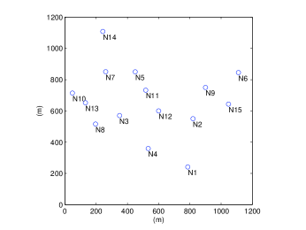
Figure 5: A 15-node network example.

V-A Cutting-Plane Method

For the 15-node example in Fig. 5, the convergence process for the cutting-plane method is illustrated in Fig. 6.

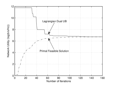
Figure 6: Convergence behavior of the cutting-plane method

The optimal objective value for this 15-node example is 6.72. The optimal flows for sessions N14 to N1, N6 to N10, and N5 to N4 are $9.17$ bps/Hz, $9.30$ bps/Hz, and $9.93$ bps/Hz, respectively. It can be observed that the cutting-plane algorithm is very efficient: It converges with approximately 160 cuts. As expected, the duality gap is zero because the convexity of the transformed equivalent problem based on dual MIMO-MAC.

V-B Subgradient Method

For the 15-node example in Fig. 5, the convergence process for the subgradient method is illustrated in Fig. 7.

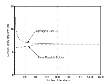
Figure 7: Convergence behavior of the subgradient method

The step size selection is $\lambda_{k}=0.1/k$. The subgradient method also achieves the same optimal solution and objective value when it converges. However, it is seen that the subgradient algorithm takes approximately 1600 iterations to converge, which is much slower than the cutting-plane method. This is partially due to the heuristic nature in step size selection (cannot be too large or too small at each step). It is also partially due to the cumbersomeness in recovering the primal feasible solution in the subgradient method. In this example, the dual upper bound takes approximately 1050 iterations to reach near the optimal. However, the near-optimal primal feasible solution cannot be identified until after 1500 iterations.

V-C Comparison between BC and TDM

We now study how much performance gain we can get by using Gaussian vector broadcast channel technique as opposed to the conventional time-division (TDM) scheme. The cross-layer optimization problem of MIMO-based mesh networks over TDM scheme is also a convex problem. Thus, the basic Lagrangian dual decomposition framework and gradient projection technique for the link layer subproblem are still applicable. The only difference is in the gradient computation, which is simpler in TDM case. For the same 15-node network with TDM, we plot the convergence process of the cutting-plane algorithm in Fig. 8.

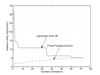
Figure 8: The convergence behavior in TDM case

In TDM case, the optimal objective value is 5.01. For this example, we have $34.4\%$ improvement by using DPC.

VI Related Work

Despite significant research progress in using MIMO for single-user communications, research on multi-user multi-hop MIMO networks is still in its inception stage. There are many open problems, and many areas are still poorly understood [19]. Currently, the relatively well-studied research area of multi-user MIMO systems are cellular systems, which are single-hop and infrastructure-based. For multi-hop MIMO-based mesh networks, research results remain limited. In [20], Hu and Zhang studied the problem of joint medium access control and routing, with a consideration of optimal hop distance to minimize end-to-end delay. In [21], Sundaresan and Sivakumar used simulations to study various characteristics and tradeoffs (multiplexing gain vs. diversity gain) of MIMO links that can be leveraged by routing layer protocols in rich multipath environments to improve performance. In [22], Lee et al. proposed a distributed algorithm for MIMO-based multi-hop ad hoc networks, in which diversity and multiplexing gains of each link are controlled to achieve the optimal rate-reliability tradeoff. The optimization problem assumes fixed SINRs and fixed routes between source and destination nodes. However, in these works, there is no explicit consideration of per-antenna power allocation and their impact on upper layers. Moreover, DPC in cross-layer design has never been studied either.

VII Conclusions

In this paper, we investigated the cross-layer optimization of DPC per-antenna power allocation and multi-hop multi-path routing for MIMO-based wireless mesh networks. Our contributions are three-fold. First, this paper is the first work that studies the impacts of applying dirty paper coding, which is the optimal transmission scheme for MIMO broadcast channels (MIMO-BC), to the cross-layer design for MIMO-based wireless mesh networks. We showed that the network performance has dramatic improvements compared to that of the conventional time-division/frequency division schemes. Second, we solved the challenging non-connvex cross-layer optimization problem by exploiting the channel duality between MIMO-MAC and MIMO-BC, and we showed that transformed problem under dual MIMO-MAC is convex. We simplified the maximum weighted sum rate problem, thus paving the way for solving the link layer subproblem in the Lagrangian dual decomposition. Last, for the transformed problem, we develop an efficient solution procedure that integrates Lagrangian dual decomposition, conjugate gradient projection based on matrix differential calculus, cutting-plane, and subgradient methods. Our results substantiate the importance of cross-layer optimization for MIMO-based wireless mesh networks with Gaussian vector broadcast channels.

References

• [1] I. E. Telatar, “Capacity of multi-antenna Gaussian channels,” European Trans. Telecomm., vol. 10, no. 6, pp. 585–596, Nov. 1999.
• [2] G. J. Foschini and M. J. Gans, “On limits of wireless communications in a fading environment when using multiple antennas,” Wireless Personal Commun., vol. 6, pp. 311–355, Mar. 1998.
• [3] T. M. Cover and J. A. Thomas, Elements of Information Theory.   New York-Chichester-Brisbane-Toronto-Singapore: John Wiley & Sons, Inc., 1991.
• [4] T. M. Cover, “Broadcast channels,” IEEE Trans. Inf. Theory, vol. 18, no. 1, pp. 2–14, Jan. 1972.
• [5] M. Costa, “Writing on dirty paper,” IEEE Trans. Inf. Theory, vol. 29, no. 3, pp. 439–441, May 1983.
• [6] H. Weingarten, Y. Steinberg, and S. Shamai (Shitz), “The capacity region of the Gaussian multiple-input multiple-output broadcast channel,” IEEE Trans. Inf. Theory, vol. 52, no. 9, pp. 3936–3964, Sep. 2006.
• [7] M. S. Bazaraa, J. J. Jarvis, and H. D. Sherali, Linear Programming and Network Flows.   New York-Chichester-Brisbane-Toronto-Singapore: John Wiley & Sons Inc., 1990.
• [8] S. Vishwanath, N. Jindal, and A. Goldsmith, “Duality, achievable rates, and sum-rate capacity of MIMO broadcast channels,” IEEE Trans. Inf. Theory, vol. 49, no. 10, pp. 2658–2668, Oct. 2003.
• [9] P. Viswanath and D. N. C. Tse, “Sum capacity of the vector Gaussian broadcast channel and uplink-downlink duality,” IEEE Trans. Inf. Theory, vol. 49, no. 8, pp. 1912–1921, Aug. 2003.
• [10] W. Yu, “Uplink-downlink duality via minimax duality,” IEEE Trans. Inf. Theory, vol. 52, no. 2, pp. 361–374, Feb. 2006.
• [11] M. S. Bazaraa, H. D. Sherali, and C. M. Shetty, Nonlinear Programming: Theory and Algorithms, 3rd ed.   New York, NY: John Wiley & Sons Inc., 2006.
• [12] S. Ye and R. S. Blum, “Optimized signaling for MIMO interference systems with feedback,” IEEE Trans. Signal Process., vol. 51, no. 11, pp. 2839–2848, Nov. 2003.
• [13] J. R. Magnus and H. Neudecker, Matrix Differential Calculus with Applications in Statistics and Economics.   New York: Wiley, 1999.
• [14] S. Haykin, Adaptive Filter Theory.   Englewood Cliffs, NJ: Prentice-Hall, 1996.
• [15] S. Boyd and L. Xiao, “Least-squares covariance matrix adjustment,” SIAM Journal on Matrix Analysis and Applications, vol. 27, no. 2, pp. 532–546, Nov. 2005.
• [16] J. Malick, “A dual approach to semidefinite least-squares problems,” SIAM Journal on Matrix Analysis and Applications, vol. 26, no. 1, pp. 272–284, Sep. 2005.
• [17] J.-B. Hiriart-Urruty and C. Lemaréchal, Fundamentals of Convex Analysis.   Berlin: Springer-Verlag, 2001.
• [18] H. D. Sherali and G. Choi, “Recovery of primal solutions when using subgradient optimization methods to solve Lagrangian duals of linear programs,” Operations Research Letters, vol. 19, no. 3, pp. 105–113, Sep. 1996.
• [19] A. Goldsmith, S. A. Jafar, N. Jindal, and S. Vishwanath, “Capacity limits of MIMO channels,” IEEE J. Sel. Areas Commun., vol. 21, no. 1, pp. 684–702, Jun. 2003.
• [20] M. Hu and J. Zhang, “MIMO ad hoc networks: Medium access control, saturation throughput, and optimal hop distance,” Special Issue on Mobile Ad Hoc Networks, Journal of Communications and Networks, pp. 317–330, Dec. 2004.
• [21] K. Sundaresan and R. Sivakumar, “Routing in ad hoc networks with MIMO links,” in Proc. IEEE ICNP, Boston, MA, U.S.A., Nov. 2005, pp. 85–98.
• [22] J.-W. Lee, M. Chiang, and A. R. Calderbank, “Price-based distributed algorithms for rate-reliability tradeoff in network utility maximization,” IEEE J. Sel. Areas Commun., vol. 24, no. 5, pp. 962–976, May 2006.