Photometry of the Globular Cluster NGC 5466: Red Giants and Blue Stragglers

Abstract

We present wide-field $BVI$ photometry for about 11,500 stars in the low-metallicity cluster NGC 5466. We have detected the red giant branch bump for the first time, although it is at least 0.2 mag fainter than expected relative to the turnoff. The number of red giants (relative to main sequence turnoff stars) is in excellent agreement with stellar models from the Yonsei-Yale and Teramo groups, and slightly high compared to Victoria-Regina models. This adds to evidence that an abnormally large ratio of red giant to main-sequence stars is not correlated with cluster metallicity. We discuss theoretical predictions from different research groups and find that the inclusion or exclusion of helium diffusion and strong limit Coulomb interactions may be partly responsible.

We also examine indicators of dynamical history: the mass function exponent and the blue straggler frequency. NGC 5466 has a very shallow mass function, consistent with large mass loss and recently-discovered tidal tails. The blue straggler sample is significantly more centrally concentrated than the HB or RGB stars. We see no evidence of an upturn in the blue straggler frequency at large distances from the center. Dynamical friction timescales indicate that the stragglers should be more concentrated if the cluster’s present density structure has existed for most of its history. NGC 5466 also has an unusually low central density compared to clusters of similar luminosity. In spite of this, the specific frequency of blue stragglers that puts it right on the frequency – cluster $M_{V}$ relation observed for other clusters.

1 Introduction

The luminosity function (LF) is an observational tool used for analyzing the post-main sequence evolutionary phases of low-mass ($\approx$ 0.5-0.8$M_{\sun}$) metal-poor stars in Galactic globular clusters (GGC). Because of their age and richness, GGC typically contain hundreds of stars that have evolved off the main sequence. The numbers of stars in evolved phases are directly related to the evolutionary timescales and fuel consumed in each phase (Renzini & Fusi Pecci, 1988), so that they present us with an opportunity to test this aspect of stellar evolution models.

The results of the most stringent tests have been mixed. Repeated studies of the metal-poor cluster M30 (Bolte, 1994; Bergbusch, 1996; Guhathakurta et al., 1998; Sandquist et al., 1999) have found an excess number of red giant branch (RGB) stars relative to main sequence (MS) stars. Stetson (1991) also uncovered an apparent excess of stars in a combined LF of the metal-poor clusters M68, NGC 6397, and M92. However, the LFs of more metal-rich clusters show no discrepancy (M5: Sandquist et al. 1996; M3: Rood et al. 1999; M12: Hargis, Sandquist, & Bolte 2004). In a survey of 18 clusters, Zoccali & Piotto (2000) found good agreement with model predictions with the possible exception of clusters at the high metallicity end.

In this paper we present $BVI$ photometry of NGC 5466, a high galactic latitude globular cluster ($l=42.2\arcdeg$ and $b=73.6\arcdeg$), located in the constellation of Boötes ($\alpha=14^{h}05^{m}27\fs 4$, $\delta=+28\arcdeg 32\arcmin 04\arcsec$ at a distance of R=15.9 kpc; Harris 1996). NGC 5466 is a loose cluster ($r_{c}=1\farcm 64$) with extremely low metallicity ([Fe/H]$=-2.22$) and subject to little or no reddening, $(E(B-V)\simeq 0)$ (Harris, 1996).

In §2, we describe the process leading to the calibrated photometry, and compare with previous studies of the cluster. In §3, we compare the observed color-magnitude diagram and observed luminosity function with theoretical models, focusing on the relative number of stars on the lower RGB and around the MS turnoff. Finally, in §4, we present a new examination of the blue straggler population of NGC 5466.

2 Observations and Data Reduction

The data used in this study were obtained with the Kitt Peak National Observatory (KPNO) 0.9 m telescope ($0\farcs 68$ pix^-1) on the nights of UT dates 1995 May 4, May 5, and May 9. A complete list of the image frames, exposure times, and observing conditions is given in Table 1.

The images obtained on the three nights were processed using IRAF tasks and packages. The reduction involved subtraction and trimming of the overscan region of all images, subtraction of a master bias frame from flats and object frames, and flat fielding of the object frames using images taken at twilight. Profile-fitting photometry was done using the DAOPHOTII/ALLSTAR programs (Stetson, 1987).

We also reduced archival ground-based photometry of the cluster core taken with the High-Resolution Camera (HRCam) on the 3.6 m Canada-France-Hawaii Telescope (CFHT). The $V$ and $I$ images were taken 30 and 31 May 1992 (observers J. Heasley and C. Christian), and have not previously been described in the literature. The CCD images had 1024 $\times$ 1024 pixels, 0$\farcs$13 per pixel, and excellent seeing (0.4 - 0.5 arcsec). The images were reduced using the archived bias and twilight flat frames, and following a procedure similar to that for the KPNO data. This allowed us to get excellent photometry to 2 magnitudes below the turnoff in the cluster core. These images were used entirely for blue straggler identification (see §4).

2.1 Calibration against Primary Standard Stars

The conditions at KPNO on 1995 May 9 were photometric, and Landolt standard star fields were observed at a range of air masses to determine photometric transformation coefficients. The standard values used for the calibration were chosen from the large compilation of Stetson (2000), which is set to be on the same photometric scale as the earlier Landolt (1992) values.

We conducted photometry on the standard stars and isolated cluster stars using multiple synthetic apertures. We then used the DAOGROW (Stetson, 1990) program to construct growth curves to extrapolate measurements to a common aperture size. Using the CCDSTD program, the standard star transformation equations were found to be:

$$b=B+a_{o}+(-0.069\pm 0.005)(B-V)+(0.255\pm 0.014)(X-1.0)$$

$$v=V+b_{o}+(0.027\pm 0.004)(B-V)+(0.172\pm 0.010)(X-1.0)$$

$$i=I+c_{o}+(-0.013\pm 0.005)(V-I)+(0.145\pm 0.018)(X-1.0)$$

where $X$ is the airmass, $v$, $b$ and $i$ are instrumental magnitudes, and $V$, $B$, and $I$ are standard magnitudes. These calibration equations are different than those used for our analysis of M10 Pollard et al. (2005) and M12 Hargis et al. (2004), which were observed on the same night, because our $I-$band exposures did not go as deep as the $B$ and $V$ exposures. As a result, the $(B-V)$ color was a better choice for calibrating the $V$ photometry down to our faintest observed stars. The calibrated measurements for the standard stars are compared with catalogue values in Fig. 1.

We note that there is slight evidence of trend in the residuals for the $I$ band versus magnitude, which might indicate nonlinearity. This impression is caused by one observation of the PG1323-086 field. We did, however, have an additional observation of the same field on the same night having the same exposure time that does not show the same (small) trend. Because we do not have any reason to eliminate the frame and because its elimination has a minimal effect on the transformation coefficients, we have decided to retain the measurements from the image.

2.2 Calibration against Secondary Standard Stars

Aperture photometry for 165 cluster stars was used to calibrate the point-spread function (PSF) photometry for the cluster. These secondary standard stars were chosen based on relatively low measurement errors and location in relatively uncrowded regions of the cluster. They were chosen from the asymptotic giant branch (AGB), upper RGB, and horizontal branch (HB) of the cluster in order to cover the entire range of colors covered by cluster stars.

The PSF-fitting photometry for the three nights of data was combined and averaged after zero-point differences among the frames had been determined and corrected. The zero-point corrections to the standard system were determined after fixing the color-dependent terms at the values measured in the primary standard star calibration. (This was also done in our studies of M10 and M12.) In Fig. 2, it can be seen that this procedure does not introduce systematic color- or magnitude-dependent errors.

2.3 Comparison with Previous Studies

We compared our photometric data set to those of Jeon et al. (2004), Rosenberg et al. (2000), and Stetson (2000). The magnitude and color comparisons ($BVI$ in this study versus $VI$ in Stetson and Rosenberg et al., and $BV$ in Jeon et al.) as function of magnitude and color are shown in Figs. 3 – 5. Though our calibrated magnitudes are slightly brighter than those of Stetson (2000), the differences are small, and there is no color trend. The offsets compared to the Rosenberg et al. (2000) are larger, but again there are no clear color trends. The offsets compared to the Jeon et al. (2004) data are also significant, but more notable are slight trends with color.

2.4 Calculation of the Luminosity Function

Artificial star tests were performed to empirically measure the precision of our photometry and to correct for incompleteness in the detection of stars. We followed the procedure described by Hargis et al. (2004) for the calculation of incompleteness corrections as function of position and magnitude.

The inputs used for producing the artificial star tests were the reduced $B$ and $V$ CCD frames, PSFs for each object frame, fiducial lines, and an estimate for the initial LF (Sandquist et al., 1996). Artificial stars were randomly placed in cells on a spatial grid and the entire grid was then shifted randomly from run to run in order to ensure the whole imaged field was tested (Piotto & Zoccali, 1999). Each star was placed in a consistent position relative to the cluster center on each image. If a detected star was found to coincide with the input position of an artificial star, it was added to the archive. The new images were reduced using the same procedure applied to the original data set. In this study, a total of 100,000 artificial stars from 50 separate runs were added. The number of artificial stars per trial was chosen so that the effects of crowding on the photometry was qualitatively unchanged.

The recovered artificial stars were used to calculate 1) median magnitude and color biases ($\delta_{V}$ and $\delta_{B-V}$, where $\delta=\mbox{median}[output-input]$), 2) median external error estimates ($\sigma_{ext}(V)=\mbox{median}[\delta_{V}-\mbox{median}(\delta_{V})]/0.6745$ and $\sigma_{ext}(B-V)$), and 3) total recovery probabilities ($F(V)$, which is the fraction of the stars that were recovered with any output magnitude) in bins according to projected radius and magnitude. The values for the above quantities are plotted in Figs.6 – 8.

Finally, an initial estimate of the “true” LF and the error distribution, magnitude biases and the total recovery probability ($F$) were used to compute the completeness fraction $f$ (the ratio of the predicted number of stars to the actual number of observed stars). The completeness fraction results are shown in Figure 9. We then interpolated to compute $f$ for the radial distance and magnitude of each detected star. For each observed star $f^{-1}$ was added to the appropriate magnitude bin to determined the observed LF. (Note that the completeness fraction was set to 1.0 for star brighter than the turnoff.) The observed LF along with the upper and lower 1 $\sigma$ error bars on log $N$ are listed in Table 2.

3 Discussion

3.1 Reddening, Metallicity, Distance Modulus, and Age

Because NGC 5466 resides at high galactic latitude, it suffers little if any reddening. Though Schlegel et al. (1998) found a reddening of $E(B-V)=0.02$ from the maps of dust IR emission, we adopted $E(B-V)=0.0$ (Rosenberg et al., 2000). For our interests in this paper, the small difference is of small importance. Most of the comparisons below between observations and theory are relative, in which reference points (like the turnoff) are used to determine magnitude and/or color shifts. This has the benefit of minimizing the influence of uncertainties in reddening and distance modulus (see below).

As for abundances, there is only one high-resolution measurement for a cluster star, and it is for the anomalous Cepheid V19. McCarthy & Nemec (1997) find [Fe/H]$=-1.92\pm 0.05$, while Pritzl et al. (2005) find [Fe/H]$=-2.05$ using the same data. Typically quoted metallicity values include [Fe/H] $=-2.17$ (Zinn, 1980) from photoelectric photometry of integrated light in selected filter bands, and [Fe/H] $=-2.22$, which was derived by Zinn & West (1984) (ultimately from low-resolution spectral scans by Searle & Zinn 1978). When converted to the widely-used metallicity scale of Carretta & Gratton (1997), this becomes [Fe/H] $=-2.14$. More work could certainly be done on the composition of NGC 5466 stars, but the evidence so far points to an abundance [Fe/H] $\lesssim-2.0$. Though the range in the above quoted metallicity values is relatively large for a globular cluster, the exact value is not critical for our purposes since we will primarily be concerned with relative comparisons.

Our photometry does not extend faint enough to derive a new distance modulus from subdwarf fitting to the main sequence. Harris (1996) obtained $(m-M)_{V}=16.0$ by calibrating the observed luminosity level of the horizontal branch with the relation $M_{V}(HB)=0.15\mbox{[Fe/H]}+0.80$ and adopting a reddening, $E(B-V)$=0.0 and a metallicity, [Fe/H]=$-2.22$. Ferraro et al. (1999) determined distance moduli $(m-M)_{V}=16.16$ from their zero-age HB estimate, assuming no reddening and metallicity on the Carretta & Gratton (1997) scale. We will consider distance moduli in this range.

Most previous age estimates of NGC 5466’s age have it older than the recent determination of the age of the universe ($13.7^{+0.13}_{-0.17}$ Gyr) obtained by the Wilkinson Microwave Anisotropy Probe (WMAP) team (Spergel et al., 2006). Recent homogeneous studies of GGC indicate that NGC 5466 is coeval with clusters of similar metallicity (Salaris & Weiss, 2002; Rosenberg et al., 2000). As a result, we will primarily consider ages in the range of 12 to 13 Gyr.

3.2 The Color-Magnitude Diagram

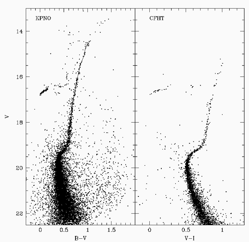
Figure 10: Color-magnitude diagrams for all stars measured in the KPNO and CFHT images. The $BV$ fiducial (Table 3) is also plotted in the left panel.

The color-magnitude diagrams (CMDs) for NGC 5466 show well-defined RGB, AGB, and HB sequences (see Fig. 10), and stars extending from the tip of the RGB down to $V\approx 22.5$. Fiducial sequences for the MS and lower RGB were determined from the mode of the color distribution of stars in magnitude bins. The SGB position was determined using the magnitude distribution of the stars in color bins. The fiducial line for the rest of the RGB was obtained from the mean color of stars in magnitude bins. The fiducial points are listed in Table 3.

A comparison of the fiducial points derived for NGC 5466 with theoretical isochrones for a range of ages from the Teramo (Cassisi et al., 2004), Victoria-Regina (VandenBerg et al., 2006), and Yonsei-Yale (Demarque et al., 2004) groups is displayed in Figures 11 and 12. The isochrones have been shifted in color and magnitude (aligning the turnoff colors and the magnitudes of the main sequence point 0.05 mag redder than the turnoff) according to the technique of Vandenberg et al. (1990). This has the advantage of removing some of systematic uncertainties associated with the color-$T_{eff}$ transformations. [In our comparisons, we found that the Yonsei-Yale models could not match the fiducial line for any reasonable set of input parameters when the transformations of Lejeune et al. (1998) were used. Therefore, we only utilize models using the Green, Demarque, & King (1987) transformations. Even then, we could not find a match with the slope of the upper giant branch for reasonable metallicities ([Fe/H] $\lesssim-1.9$).] On the whole, the shape of the fiducial matches the models well on the main sequence, subgiant branch, and lower giant branch. Neither the Teramo nor the Victoria-Regina models include element diffusion processes, while the Yonsei-Yale isochrones only include He diffusion. However, differences in $T_{eff}$-color transformations are likely to be the cause of some of the differences seen.

3.3 The Luminosity Function

The number of stars at a given luminosity in post-main-sequence phases is directly proportional to the lifetime spent at that luminosity. It is well known that the LF of the RGB probes the chemical stratification inside a star because the hydrogen abundance being sampled by the thin hydrogen-fusion shell affects the rate of evolution, and hence star counts on the RGB (Renzini & Fusi Pecci, 1988). Setting aside the short pause at the RGB bump, RGB evolution accelerates in a very regular way that is ultimately related to the structure of degenerate core. The relationship between core mass and radius forces the fusion shell to function at strictly controlled density and temperature conditions, which leads to a relationship between core mass and luminosity. This causes the LF to be particularly sensitive to certain physical details, which we discuss in §3.3.1 below.

Fig. 13 shows the observed luminosity function compared to theoretical LFs for the labeled values of metallicity, exponent of the initial mass function, and a range of age estimates for NGC 5466, assuming our preferred distance modulus $(m-M)_{V}=16.00$. The theoretical models were normalized to the observed LF at $V\approx 21.3$ (sufficiently faint that stellar evolution effects are minimized). The models agree well with the observed LF, implying an age of approximately 12 - 13 Gyr.

3.3.1 Relative RGB and MS Numbers

Gallart et al. (2005) recently discussed theoretical luminosity functions calculated by different groups. One of the primary differences they noted was in the number of giant stars relative to main sequence stars. In order to show these differences in a parameter-independent way, we follow the method of Vandenberg et al. (1990). In Fig. 14, the theoretical LFs were shifted so that a point on the main sequence 0.05 mag redder than the turnoff color point matched the corresponding point on the cluster fiducial line. The reason for using the point ($V_{TO+0.05}$) rather than the MSTO itself is that the MS has a significant slope and curvature at this point, making it possible to accurately measure the point in both observational data and isochrones (Vandenberg et al., 1990). The theoretical models were normalized to the two bins in the observed LF on either side of the turnoff ($V=19.83$ and 20.13). As can be seen, age-related differences between the theoretical LFs nearly disappear when this procedure is applied (see also Stetson 1991; Vandenberg et al. 1998). However, when different sets of models are compared, there are small differences in the number of RGB stars relative to MS stars, with the Victoria-Regina models predicting the smallest number of giants and the Yonsei-Yale models predicting the largest.

To quantify the differences, we computed the ratio of the number of stars on the lower giant branch to the number of stars near the main sequence. Pollard et al. (2005) introduced this ratio and showed that it is insensitive to age and heavy-element abundance. For the main sequence population, we used star counts in the two bins on either side of the turnoff ($19.682<V<20.282$), and for the red giant branch we used the counts in the range $16.982<V<18.482$. We derived model values from the same magnitude ranges relative to the $V_{TO+0.05}$ point on the main sequence. Values are compared in Table 4. The error in the observed value is dominated by Poisson statistical scatter. The Yonsei-Yale models are in best agreement with the observations, the Victoria-Regina models are out of agreement by more than 2 $\sigma$, and the Teramo models are in between.

It is worth examining the possible causes of this difference both because it may help improve the physics inputs for the models and because red giant stars are some of the largest contributors to the integrated light of old stellar populations. Gallart et al. (2005) tabulated most of the main physics inputs for the most widely-used model sets. Earlier studies (Stetson, 1991; Vandenberg et al., 1998) have shown that the LF-shifting method used above eliminates nearly all sensitivity to model input parameters like mass function, age, convective mixing length, and composition inputs with the exception of helium abundance, which we examine first.

Older models (e.g. Fig. 9 of Ratcliff 1987, Fig. 7 of Stetson 1991, Fig. 3 of Vandenberg et al. 1998) seem to agree that an increase in initial helium abundance $Y$ in non-diffusive models by 0.1 results in an increase in the relative number of stars on the RGB (more precisely, a reduction in the relative number of main sequence stars) by about 0.07-0.08 in $\log N$. The Teramo models ($Y=0.245$) predict about 12% more giant stars relative to main sequence stars compared to the Victoria-Regina models ($Y=0.235$). This difference corresponds to a shift of 0.05 in $\log N$, which is about an order of magnitude too large for the helium abundance difference.

The Yonsei-Yale models have the lowest assumed helium abundance ($Y=0.23$), but are the only set of the three that include helium diffusion. The inclusion of helium diffusion reduces the age derived from the turnoff of a globular cluster by about 10-15% (Proffitt & Vandenberg, 1991; Straniero et al., 1997; VandenBerg et al., 2002), thanks to the inward motion of helium. According to theoretical models (e.g. Fig. 8 of Proffitt & Vandenberg 1991), diffusion has a small effect on the LFs ($\sim$ a few times $10^{-2}$ in $\log N$, increasing for increasing age), but it does increase the number of giants relative to MS stars. He diffusion reduces the total core hydrogen fuel supply available to an MS star, but in itself this does not strongly modify the LF, just changes the brightness of the turnoff. This magnitude change is eliminated in our LF shifting procedure. The chemical composition profile left in the star after it leaves the main sequence has a greater impact. Diffusion reduces the H abundance in the fusion regions, thereby decreasing the evolutionary timescale. According to the models of Proffitt & Michaud (1991), the changes to the He abundance profile are most considerable immediately below the surface convection zone, and just outside the nuclear fusion regions (where the composition gradient slows the inward settling of helium). However, over most of the star, the changes in $Y$ are limited to 0.01 - 0.02. Because the core portion of the composition profile is consumed on the subgiant branch, the evolution timescales for giant stars are only affected in a minor way, and the appearance of a deep convection zone on the lower giant branch wipes out most of the effects of diffusion for the upper giant branch evolution.

In spite of this, the Yonsei-Yale models have almost 23% more giants than the Victoria-Regina models, and more than 9% more giants than the Teramo models (relative to MS stars). The lower helium abundance in the Yonsei-Yale models compared to the other models should partially counteract what effects helium diffusion might have had on the RGB/MS ratio as well. Thus, it appears that neither He abundance nor He diffusion can completely explain the differences between the Yonsei-Yale models and the other groups.

We can ask whether the LFs show similar disagreements at other metallicities. Hargis et al. (2004) made comparisons between the Victoria-Regina and Yonsei-Yale theoretical LFs and observational LFs for the clusters M3 (Rood et al., 1999), M5 (Sandquist et al., 1996), M12, and M30. The overall impression from those comparisons was again that the Yonsei-Yale models (having He diffusion) predict more giant stars relative to main-sequence stars than do the Victoria-Regina models. In Fig. 15, we compare the LFs for these clusters with the Teramo models. The degree of agreement or disagreement can be quantified with number ratios of lower RGB and MSTO stars, similar to the ones we computed earlier for comparisons with NGC 5466. Our calculations are shown in Table 4. As can be seen, uncertainties in the metallicity scale have some effect on the comparisons with the observations. The Carretta & Gratton (1997) scale has higher [Fe/H] values than the Zinn & West (1984) scale, and thus results in lower number ratios.

Fig. 16 shows the results of comparing the observed ratios with the models for different [Fe/H] scales. On the Zinn & West 1984 scale (right panels), the observed values seem to be in agreement to within about $1-1.5\sigma$ for most of the models, with the exception of the the lowest metallicity clusters (M30 and NGC 5466) and the lowest helium abundance (Victoria-Regina) models. On the Carretta & Gratton 1997 scale, the Yonsei-Yale models have the best overall agreement, although the Teramo models only deviate noticeably for the lowest metallicity clusters. The Victoria-Regina models predict too few giants for all of the clusters.

The differences from model to model (as opposed to models versus observation) point toward deficiencies elsewhere in the physics or computational algorithms used in the stellar evolution codes. The RGB LF is a robust prediction of the models because there is a strong core mass — luminosity relationship: the conditions in the hydrogen fusion shell of the giant are strongly dependent on the structure of the degenerate core and are almost independent of the details of the mass or structure of the envelope. As a result of this, we can focus on factors affecting core structure. (As a non-standard physics example, Vandenberg et al. 1998 describe the way in which core rotation relieves a giant star of some of the need to support itself by gas pressure, which reduces the core temperature and lengthens the evolutionary timescale.) Because model-to-model differences appear even on the faint end of the giant branch, we can set aside factors that only become important to the structure of the star near the tip of the giant branch [such as neutrino losses and conductive opacities; see Bjork & Chaboyer 2006, for example], even though there are significant theoretical uncertainties in these quantities. Nuclear reaction rates in the fusion shell can also be neglected, partly because the uncertainties in the reactions appear to be relatively small Adelberger et al. (1998), but also because small changes in the reaction rates require only tiny changes in the shell temperature to get the same energy production. This leads us to examine the equation of state (EoS) in the core.

Although the behavior of degenerate electrons is thought to be very well understood, their interactions with nuclei can have a measureable effect on the pressure. Particles of like charge tend to cluster together, which modifies the free energy of the gas and reduces the gas pressure for given density and temperature. Harpaz & Kovetz (1988) looked at the effects of the inclusion of Coulomb interactions on giant stars, and their results are corroborated by those of Cassisi et al. (2003). They found that for a given core mass the fusion shell temperature was higher when the Coulomb interactions were included, which leads to faster processing of hydrogen. Thus this is another example (like core rotation) where modification of the pressure support of the core affects the evolutionary timescales, which results in changes to the luminosity function. The Coulomb corrections to the pressure become more important with increasing density for the core, but are small compared to the contribution of the degenerate electrons.

All of the model sets we have considered here incorporate Coulomb interactions in some form. The Teramo group used the most sophisticated “EOS1” version of the FreeEOS, which incorporates Coulomb corrections in a form that matches limits in both the weak (Debye-Hückel) and strong (once-component plasma) Coulomb interaction limits as well as (less importantly) electron exchange interactions. The strong interaction limit is most relevant for giant star cores since the strong interaction parameter

$$\Gamma=\frac{\zeta^{2}e^{2}}{r_{0}kT}\gtrsim 1,$$

where $\zeta$ is the rms nuclear charge and $r_{0}$ is the average internuclear distance.

The Yonsei-Yale group used the OPAL EoS tables (Rogers et al., 1996), but falls back on the group’s older EoS [e.g. (Guenther et al., 1992)] for conditions for high densities and temperatures outside the OPAL tables. While the most recent OPAL tables probably contain the most complete physical description of the Coulomb effect, the OPAL tables they used (Y.-C. Kim, private communication) were computed prior to recent improvements to account for relativistic electrons (Rogers & Nayfonov, 2002), and as a result cut off at $\log\rho>5.0$. The Yale EoS at higher densities only includes the Coulomb effect in the weak Debye-Hückel limit, which for the highest densities in the core. The Victoria-Regina models also use a modified version of the EFF EoS (Eggleton et al., 1973), with a correction for Coulomb corrections in the weak Debye-Hückel limit (VandenBerg et al., 2000).

The differences in the implementation of the Coulomb effect may explain the fact that the Teramo models generally predict more giants (relative to the main sequence) than the Victoria-Regina models do. However, the smaller Coulomb corrections in the Yonsei-Yale models would tend to result in fewer giants than the Teramo models (although the effects of helium diffusion work in the opposite direction). So, we are unable to completely reconcile the differences in the luminosity functions from the three groups.

Obviously more detailed study is needed by all of the modelling groups to identify the causes of the differences, but such a study is beyond the scope of this paper. Still, we believe that helium diffusion and strong interaction Coulomb corrections are physical effects that should be considered first. There is, for example, good evidence from helioseismology for helium diffusion in the Sun Bahcall et al. (1995), despite the surface convection and meridional flow (e.g., Hathaway 1996). It is expected that helium diffusion should also act in globular cluster stars. A detailed study of the effect of equation of state uncertainties has yet to be done [see, for example, Bjork & Chaboyer (2006) for a study of uncertainties in other physical inputs]. Use of FreeEoS would make a study of equation of state effects most stringent since it appears to be capable of modelling the most sophisticated tabular EoS (OPAL), while also having the flexibility to allow individual bits of the physics to be “turned off”.

As a final warning about the observations, we should remember the LF of the cluster M10. Pollard et al. (2005) found that unusual variations in numbers of RGB stars at different brightness levels in M10 (a virtual twin to M12). In particular there seemed to a significant excess in the number of stars near the RGB bump in brightness, while the lower RGB appeared normal (compared to Victoria-Regina and Yonsei-Yale models). A similar excess may be present in the RGB LF of M13 (Cho et al., 2005). These kinds of variations cannot be explained by the “global” physics that should apply to all globular cluster stars. These anomalies point toward fluctuations in the stellar initial mass function or composition-dependent effects.

3.3.2 The RGB Bump

A second feature of the LF presented here is a noticeable RGB bump. Typically, the RGB bump appears as a peak in the differential LF and as a change of slope in the cumulative LF (CLF). The bump provides a measure of the maximum depth reached by the outer convection zone during first dredge-up since it is the result of a pause in the star’s evolution when the shell fusion source begins consuming material of constant, lower helium content (Fusi Pecci et al., 1990). Unfortunately, the number of stars occupying the bump gets smaller and the luminosity of the bump increases as the metallicity of the cluster decreases, making the bump harder to detect in metal-poor clusters. A small peak appears in our differential LF at $V\approx 16.2$, and a significant ($2.5-3.5\sigma$) change in slope occurs at the same position as the peak in the differential LF, as shown in Fig. 17.

The relative brightness of the bump can be measured by comparing to the $V$-magnitude of the HB at the level of the RR Lyrae instability strip $\Delta V^{bump}_{HB}=V_{bump}-V_{HB}$ (Ferraro et al., 1999). This indicator is a function of the total metallicity and the age of the cluster: an increase in metallicity and/or a decrease in age are accompanied by a decrease in luminosity of the bump (Ferraro & Montegriffo, 2000). We find $V_{bump}=16.20\pm 0.05$ mag, and $V_{HB}=16.52\pm 0.11$ (from interpolation between the average magnitudes of non-variable HB stars at the blue and red ends of the RR Lyrae instability strip), giving $\Delta V^{bump}_{HB}=-0.32\pm 0.12$. In the compilation of Ferraro et al. (1999), a zero-age HB reference point was calculated using the relation $V_{ZAHB}=V_{HB}+0.106\mbox{[Fe/H]}^{2}+0.236\mbox{[Fe/H]}+0.193$. Ferraro et al. found $V_{ZAHB}=16.62\pm 0.10$, which is consistent with the value obtained here ($V_{ZAHB}=16.65\pm 0.11$). Our value of $\Delta V_{ZAHB}^{bump}=-0.45\pm 0.12$ is considerably lower than tabulated values for other clusters with similar metallicities (M68: $-0.60\pm 0.07$; M92: $-0.65\pm 0.12$; M15: $-0.65\pm 0.09$). In a separate compilation, Zoccali et al. (1999) measured a smaller value $\Delta V_{ZAHB}^{bump}=-0.45\pm 0.11$ for M15, in better agreement with the value for NGC 5466. (The difference is primarily because Zoccali et al. measured the bump position to be 0.16 mag fainter than Ferraro et al..) Clearly there is still some need for more precise comparisons of bumps in metal-poors clusters with theory.

We believe, however, that the brightness of the bump should ultimately be judged using hydrogen-fusing stars as references because it avoids any effects of the poorly-understood physical processes (such as the helium flash and/or mass loss) associated with the creation of an HB star. Using the cluster LF (as seen in Figure 14), we again find that the observed RGB bump is fainter than model values by at least 0.3 mag when the models are shifted to match the cluster’s main sequence. Hargis et al. (2004) did similar comparisons between theoretical models and luminosity functions for M3, M5, M12, and M30 taken from the literature. With the exception of M30 (because the bump could not be identified), the position of the bump relative to the turnoff region agreed well with theory. NGC 5466 is thus the most metal-poor cluster this comparison has been done for. So at present we are left with the question of whether this might result from the cluster’s low metallicity, or whether we have been the unfortunate victims of a fluctuation in the number of giant stars in this low-mass cluster. We therefore encourage the examination of the luminosity function of more massive metal-poor clusters to settle the question.

3.3.3 Mass Function Exponent

Two recent papers (Belokurov et al., 2006; Grillmair & Johnson, 2006) reported the discovery of tidal streams covering many degrees around NGC 5466 in Sloan Digital Sky Survey images. Gnedin & Ostriker (1997) examined the Milky Way globular clusters and found NGC 5466 to be a cluster that has probably been strongly affected by disk shocking in the recent past. In our examination of the LF, we found a rather low value for the global main sequence mass function slope. The mass function for a cluster is typically expressed as a power law ($N(M)\propto M^{-(1+x)}$), where the slope $x=1.35$ is the standard Salpeter value. Generally, the present-day power-law index $x$ varies from cluster to cluster. The mass function slopes that best fit the upper LF of NGC 5466 around and above the MSTO have $-1\lesssim x\lesssim 0$. (Note that the best fit slope does depend on the models being used: the Yonsei-Yale models require a flatter slope than the Victoria-Regina and Teramo models.) Such a shallow mass function slope is unusual for a metal-poor cluster. For example, the cluster NGC 5053 has similar metallicity, position relative to the galactic center and plane, and density structure, but still has a steep $x\sim 2$ mass function (Fahlman et al., 1991). Djorgovski et al. (1993) found that mass function slopes in the range of $0.5\leq\frac{M}{M_{\sun}}\leq 0.8$ are influenced primarily by the cluster’s position in the galaxy, and to some extent by cluster metallicity. Based on both of those factors, NGC 5466 should have a larger mass function slope ($x\sim 3$ according to the multivariate formula in Djorgovski et al. 1993). Like other halo clusters, NGC 5466’s orbit is quite eccentric and will take the cluster more than 30 kpc away from the Galactic center (Dinescu et al., 1999), but it is currently on its way back into the halo after two relatively recent passes through the Galactic disk. Recent losses of low-mass stars may explain the recent identification of strong tidal tails near the cluster by Belokurov et al. (2006).

4 Blue Stragglers

Blue stragglers (BSSs) were first identified by Sandage (1953) in the globular cluster M3. These stars are more massive than the turnoff mass and occupy the space in the CMD just bluer and brighter than the MSTO. Blue stragglers are found in clusters, and relatively more frequently in lower-luminosity clusters (Ferraro et al., 1993; Preston & Sneden, 2000; Piotto et al., 2004; Sandquist, 2005). From the various models proposed for the formation mechanism of BSSs, the “collision” theory (involving strong gravitational interactions between previously unassociated single or binary stars) and the “mass-transfer” theory (in which the more massive star in a binary evolves and during its expansion transfers mass to its companion) are the strongest possibilities. There is a continuing interest in the study of BSSs because they may provide insight into the recent dynamical history of a cluster.

In order to identify BSSs over the entire observed area of the cluster out to a radius of 11$\farcm$6, we used photometry from three datasets. In the core of the cluster we used the CFHT data presented here for the first time. Outside of the CFHT field, we used the $BV$ photometry of Jeon et al. 2004, which covered a field 11$\farcm$6 on a side centered on the cluster. Finally, we used our KPNO data for the least crowded outskirts of the cluster. Even though NGC 5466 is a very low density cluster, the spatial resolution of the KPNO data was such that blends of stars would have resulted in the spurious identification of 10 objects as BSS in the intermediate portion of the field.

48 BSS candidates were identified in NGC 5466 by Nemec & Harris (1987), all located between $0\farcm 1$ and $5\farcm 6$ from the cluster center. In spite of the low cluster density, we find new BSS candidates at all radii and luminosity levels, and find several of their candidates are spurious. According to the CFHT photometry, the object with ID 45 from Nemec & Harris is a blend of several fainter stars, none of which is a BSS. In addition, IDs 6 and 24 were identified as blends of stars using the Jeon et al. (2004) dataset. Our BSS list is presented in Table 5. The list includes the nine known SX Phoenicis stars (ID 27, 29, 35, 38, 39, and 49, Nemec & Mateo 1990; ID 3 (SX Phe 3), 36 (SX Phe 2), and 50 (SX Phe 1), Jeon et al. 2004) and the three eclipsing binaries (ID 19, 30, and 31; Mateo et al. 1990). New straggler candidates were given ID numbers that build upon the Nemec & Harris (1987) list. Figure 18 shows the CMDs used to select the 94 identified BSSs in each of the three datasets.

In order to use the BSSs to constrain cluster dynamics, we compared the normalized cumulative radial distribution of the BSSs to the population of the giant branch, as shown in Fig. 19. Nemec & Harris (1987) found a 97.8% probability that their BSS sample was more centrally concentrated than red giants in the same magnitude range. Because their photometry was taken in conditions of poorer seeing (compared to our CFHT photometry and that of Jeon et al.), their samples are likely to be somewhat incomplete near the cluster center.

Our RGB sample contains 350 stars with magnitude $V<18.5$. Kolmogorov-Smirnov (K$-$S) probability tests were used to test the hypothesis that both populations were drawn from the same parent population. The K$-$S probability that the BSSs are drawn from the same radial distribution as the RGB population is $8.1\times 10^{-7}$, and $2.4\times 10^{-4}$ for the comparison with the HB population. By contrast there is a probability of 0.27 that the RGB and HB samples are drawn from the same population. The concentration of BSSs toward the cluster center as compared to the RGB and HB samples is consistent with the idea that they are more massive than individual RGB stars, and as a result have been segregated by mass deeper within the cluster potential well.

Piotto et al. (2004) recently used samples of stragglers from the cores of 56 globular clusters to show that there was a strong correlation between $F^{HB}_{BSS}=N_{BSS}/N_{HB}$ and integrated cluster $V$ magnitude, and a weaker anti-correlation with central density. Sandquist (2005) examined an additional 13 low-luminosity globular clusters using similar selection criteria. NGC 5466 is an interesting cluster in relation to these samples because it has an integrated luminosity that puts it at the faint end of the Piotto et al. sample ($M_{V_{t}}=-6.96$; Harris 1996), but with a central density that is nearly an order of magnitude lower than any of their clusters [$\log(\rho_{0}/(L_{V,\odot}\mbox{pc}^{-3}))=0.88$] but comparable to clusters in the Sandquist sample. To put NGC 5466 in the context of the Piotto et al. and Sandquist samples, we selected a subset of our BSSs that satisfied the selection criteria in those studies (brighter than the MSTO, and bluer than the MSTO by 0.05 in $B-V$ color). From mode fitting to the turnoff region in the Jeon et al. (2004) and CFHT data, we find $(B-V)_{TO}=0.367$ and $(V-I)_{TO}=0.511$. A color offset of 0.05 in $B-V$ corresponds to an offset of about 0.075 in $V-I$ (VandenBerg & Clem, 2003) for NGC 5466’s metallicity. We find that 75 BSSs are brighter than the cluster turnoff ($V_{TO}=19.99\pm 0.05$) and 0.05 bluer than the cluster turnoff in $B-V$. We have identified 97 HB stars in our datasets for NGC 5466, which gives a specific frequency $F^{HB}_{BSS}=0.77\pm 0.12$ (with the error estimate from Poisson statistics).

When compared to the Piotto et al. values (see Fig. 20), NGC 5466 falls within the general trend versus $M_{V_{t}}$ despite the cluster’s low central density. On the other hand, NGC 5466 has a lower $F^{HB}_{BSS}$ value than other clusters of similar central density (but lower total luminosity). As discussed by Sandquist (2005), this provides additional evidence that the plateau in $F^{HB}_{BSS}$ seen for clusters with $\log\rho_{0}\lesssim 2.5$ is a result of the correlation between cluster integrated magnitude and central density. The lowest luminosity clusters in the Sandquist sample (E3 and Palomar 13) have central densities comparable to that of NGC 5466, but BSS frequencies that are several times higher. Another moderate-luminosity, low-density cluster (NGC 5053; Hiner et al., in preparation) similar to NGC 5466 shows a comparably low straggler frequency. BSSs produced via purely collisional means are not likely to show this kind of behavior. More likely is the scenario proposed by Davies et al. (2004) in which binary stars that would normally produce BSSs are destroyed earlier in the cluster’s history. More direct observational support for that hypothesis is needed though — for example, a detailed study of the variation of the binary star fractions as a function of integrated cluster magnitude.

Fig. 21 shows that the number and frequency

$$R_{BSS}=\frac{N_{BSS}/N_{BSS}^{tot}}{L^{sample}/L^{sample}_{tot}}$$

of BSSs relative to the integrated $V$-band flux (derived from a King model profile) as a function of radius. Both frequencies increase toward the cluster center, and neither shows signs of rising toward larger radii. As recent studies of denser clusters show (M3: Ferraro et al. 1993; M55: Zaggia et al. 1997; 47 Tuc: Ferraro et al. 2004; NGC 6752: Sabbi et al. 2004), the BSS frequency generally decreases at intermediate radii and rises again at larger distances. However, the cluster Palomar 13 (Clark et al., 2004), which has a central density similar to NGC 5466, shows no sign of an increase in straggler frequency at large distance.

In more massive clusters, the minimum in the BSS frequency is reached approximately where the timescale for dynamical friction equals the age of the cluster (Warren et al., 2006). A similar calculation for the current structure of NGC 5466 indicates that this occurs at about 270″(about $2.8r_{c}$). This appears to be in the outer reaches of the core straggler distribution. Because it is likely that NGC 5466 has lost a significant fraction of its mass, we expect that the current density structure of the cluster has not existed throughout its history and that NGC 5466 might have been able to dynamically relax stragglers to its core from larger distances earlier in its history. This may be showing that the global BSS population differs significantly between low-density/low-mass clusters and high-density/high-mass clusters. A lack of stragglers at large distance may be signature of large-scale tidal stripping of the cluster, which would remove both stragglers that would normally have formed in primordial binaries in the outer reaches of the cluster and ones that formed in the core but were given velocity kicks into orbits that would take them into the outer reaches.

The case against a rise at large radius in Palomar 13 is stronger because the cluster has been surveyed out to 19 core radii, while in NGC 5466, we have only surveyed out to about 10 core radii (or 7.5 half-mass radii). Still, NGC 5466 probably should have an even more concentrated distribution of stragglers if its current density structure has existed for most of its history. In more massive clusters, the secondary rise in straggler frequency is observed between 8 and 10 $r_{c}$. Unfortunately, further study of the stragglers in NGC 5466 will probably be complicated by the strong tidal tails observed in the cluster.

5 Conclusions

Examinations of the luminosity functions of globular clusters continue to produce interesting tests of astrophysics. In this study, we found that NGC 5466 has a luminosity function that is in better overall agreement with theoretical models than the anomalous cluster M30, which has a similar low metallicity. In addition, we found that the relative numbers of red giant and main sequence stars may produce a fairly sensitive test of the physics near the core of red giants — specifically, helium diffusion and Coulomb interactions. However, we are not yet able to fully explain the differences between sets of theoretical models.

Recent discoveries of large tidal tails associated with NGC 5466 suggest that this cluster has been strongly disrupted by interactions with the Galaxy. Our measured flat ($-1\lesssim x\lesssim 0$) main-sequence luminosity function is unusual for a low-metallicity halo cluster. It is, however, consistent with the emerging picture of mass-segregation followed by tidal stripping.

We have thoroughly re-examined the blue straggler population in the cluster, and detected a total of 94. The radial distribution of stragglers is clearly more centrally concentrated than the RGB and HB populations. The frequency of blue stragglers in the cluster is relatively low — consistent with the observed anti-correlation between frequency and cluster luminosity, in spite of the cluster’s very low central density.

Figure 1: Photometric residuals (in the sense of this study minus those of Landolt 1992 and Stetson 2000) of primary standard stars. The median residuals are listed in the panels with the semi-interquartile range (half the magnitude difference between the 25% and 75% points in the ordered list of residuals) given in parentheses.

Figure 2: Photometric residuals (in the sense of the final PSF photometry minus standard aperture photometry values) of secondary standard stars.

Figure 3: Residuals (in the sense of this study minus Stetson 2000) from the star-by-star comparison. The median residuals are listed in the panels with the semi-interquartile range (see Fig.1) given in parentheses.

Figure 4: Residuals (in the sense of this study minus Rosenberg et al. 2000) from the star-by-star comparison. The median residuals and the plots versus color have been restricted to brighter stars ($V<20$ and $I<19$) to make the comparisons clearer. The numbers in parentheses are the semi-interquartile ranges (see Fig.1).

Figure 5: Residuals (in the sense of this study minus Jeon et al. 2004) from the star-by-star comparison. The median residuals and the plots versus color have been restricted to brighter stars ($B<20$ and $V<19.5$) to make the comparisons clearer. The numbers in parentheses are the semi-interquartile ranges (see Fig.1).

Figure 6: External $V$ magnitude errors $\sigma_{ext}(V)$ as a function of radius and magnitude determined from artificial star tests, with exponential fits shown by the solid lines.

Figure 7: Magnitude biases $\delta(V)$ determined from artificial star tests as a function of radius and magnitude.

Figure 8: Total recovery probability $F(V)$ determined from artificial star tests as a function of radius and magnitude.

Figure 9: Completeness fraction $f(V)$ determined from artificial star tests as a function of radius and magnitude.

Figure 11: Comparison of the observed fiducial sequence of NGC 5466 with the isochrones of the Teramo, Victoria-Regina, and Yonsei-Yale groups. The isochrones have been shifted horizontally so that the turnoff colors align, and shifted vertically to align the main sequence point 0.05 mag redder than the turnoff. On the giant branch, the ages increase from the reddest to the bluest isochrone.

Figure 12: Same as Fig. 11, except for more metal-rich models.

Figure 13: Comparison of the observed $V-$band LF of NGC 5466 with theoretical models of the Yonsei-Yale, Teramo, and Victoria-Regina groups assuming $(m-M)_{V}=16$.

Figure 14: Comparison of the observed $V-$band LF of NGC 5466 with theoretical models of the Victoria-Regina, Yonsei-Yale, and Teramo groups using magnitude shifts that bring the main sequence point 0.05 mag redder than the turnoff into alignment. The models have been normalized to the two bins on either side of the turnoff ($V=19.94$).

Figure 15: Comparison of the observed LFs of M3, M5, M12, and M30 with theoretical models of the Teramo group using magnitude shifts that bring the main sequence point 0.05 mag redder than the turnoff into alignment. The models have been normalized to bins on either side of the turnoff.

Figure 16: Fractional difference between the observed RGB-MS number ratios (for M5, M12, M3, M30, and NGC 5466, from left to right) and the theoretical predictions from the Yonsei-Yale, Teramo, and Victoria-Regina models. The left panels use the Carretta & Gratton (1997) metallicity scale, and the right panels use the Zinn & West (1984) scale. The sense is (observed $-$ theoretical) / observed.

Figure 17: The cumulative luminosity function for bright RGB stars derived from the photometry of Jeon et al. (2004; 286 stars) and from the KPNO dataset (338 stars) presented here. Dotted lines show fits to the data for stars above and below the position of the apparent bump.

Figure 18: Blue straggler selection for NGC 5466. The stars plotted in each panel show the entire sample used for the selection: stars from Jeon et al. (2004) in the middle panel are only those stars outside the CFHT field, and KPNO stars in the right panel are only those outside the Jeon et al. field. Open squares show stragglers identified by Nemec & Harris (1987), and open circles are new candidates.

Figure 19: Normalized cumulative radial distributions for RGB stars (dashed line), HB stars (dotted line), and BSSs (solid line).

Figure 20: Relative frequencies of blue stragglers as a function of cluster absolute magnitude and central density. The solid square is NGC 5466, the open squares are globular clusters from Sandquist (2005), and all other points are from Piotto et al. (2004). Open circles are post-core-collapse clusters. In the left panel, symbols represent clusters in different ranges of central density from the Piotto et al. sample: $\log\rho_{0}<2.8$: open triangles; $2.8<\log\rho_{0}<3.6$: filled triangles; $3.6<\log\rho_{0}<4.4$: stars; $\log\rho_{0}>4.4$: filled circles.

Figure 21: Frequency of BSS relative to the integrated $V$-band flux of detected cluster stars (top panel) and specific frequency of blue stragglers relative as a function of radius (bottom panel).

Table 1: Photometric Observation Log for NGC 5466

UT Date	Filters	$N$	Exposure Time (s)	Airmass
1995 May 4	$B$,$V$	1,1	60	1.01,1.12
1995 May 4	$B$	2	300	1.03, 1.03
1995 May 4	$B$,$V$	2,1	600	1.0,1.11,1.0
1995 May 5	$B$,$I$	2,2	300	1.03,1.01,1.02,1.01
1995 May 9	$B$,$V$,$I$	1,1,1	60	1.12,1.13,1.14

Table 2: $V$-Band Luminosity Function

$V$	$\log N$	$\sigma_{high}$	$\sigma_{low}$
13.532	0.5005	0.1761	0.3010
13.832	$-0.1015$	0.3010	1.0000
14.132	$-0.1015$	0.3010	1.0000
14.432	0.5975	0.1605	0.2575
14.732	0.8985	0.1193	0.1651
15.032	0.6767	0.1487	0.2279
15.332	0.6767	0.1487	0.2279
15.632	0.5976	0.1606	0.2575
15.932	0.8986	0.1193	0.1651
16.232	1.2410	0.0839	0.1041
16.532	1.0127	0.1063	0.1411
16.832	1.0451	0.1029	0.1351
17.132	1.3306	0.0764	0.0928
17.432	1.4432	0.0678	0.0804
17.732	1.4777	0.0728	0.0876
18.032	1.6136	0.0630	0.0738
18.332	1.7575	0.0540	0.0617
18.632	1.7577	0.0540	0.0617
18.932	1.9624	0.0433	0.0481
19.232	2.2928	0.0301	0.0324
19.532	2.5143	0.0236	0.0249
19.832	2.6996	0.0192	0.0201
20.132	2.7738	0.0178	0.0185
20.432	2.8830	0.0159	0.0165
20.732	2.9327	0.0151	0.0157
21.032	3.0036	0.0142	0.0146
21.332	3.0496	0.0137	0.0142
21.632	3.1179	0.0132	0.0136

Table 3: Fiducial sequence for NGC 5466

$V$	$B-V$	$N$
22.198	0.578	518
21.999	0.564	598
21.798	0.549	724
21.596	0.532	710
21.398	0.498	673
21.200	0.470	670
21.004	0.459	653
20.802	0.450	614
20.600	0.431	568
20.400	0.418	546
20.199	0.404	470
20.001	0.395	453
19.805	0.396	382
19.599	0.403	273
19.400	0.436	235
19.206	0.495	155
19.005	0.543	84
18.823	0.586	70
18.588	0.607	43
18.401	0.616	52
18.204	0.621	40
17.989	0.636	34
17.820	0.647	31
17.586	0.654	23
17.403	0.672	20
17.194	0.677	19
16.988	0.693	11
16.784	0.722	10
16.613	0.725	6
16.400	0.752	12
16.199	0.771	16
16.066	0.779	5
15.825	0.809	7
15.602	0.827	4
15.407	0.857	6
15.111	0.917	1
15.006	0.930	5
14.786	0.946	2
14.590	0.986	11
14.438	1.044	2

Table 4: RGB-MSTO Number Ratios

Source	TO Sample	RGB Sample	$Y$	$N_{RGB}/N_{MSTO}$	[Fe/H]
NGC 5466	$19.682<V<20.282$	$16.982<V<18.482$		$0.162\pm 0.013$
VR			0.235	0.132	$-2.22$
VR			0.235	0.130	$-2.14$
T			0.245	0.148	$-2.22$
T			0.245	0.146	$-2.14$
YY			0.230	0.162	$-2.22$
YY			0.230	0.160	$-2.14$
M3	$18.80<V<19.40$	$16.40<V<18.00$		$0.168\pm 0.008$
VR			0.235	0.170	$-1.66$
VR			0.235	0.158	$-1.34$
T			0.246	0.181	$-1.66$
T			0.248	0.170	$-1.34$
YY			0.230	0.185	$-1.66$
YY			0.230	0.162	$-1.34$
M5	$19.13<B<19.73$	$16.33<B<17.93$		$0.110\pm 0.006$
VR			0.235	0.106	$-1.40$
VR			0.235	0.097	$-1.11$
T			0.248	0.114	$-1.40$
T			0.251	0.106	$-1.11$
YY			0.230	0.119	$-1.40$
YY			0.230	0.105	$-1.11$
M12	$18.14<V<18.74$	$15.59<V<17.24$		$0.158\pm 0.011$
VR			0.235	0.144	$-1.40$
VR			0.235	0.118	$-1.14$
T			0.248	0.155	$-1.40$
T			0.251	0.144	$-1.14$
YY			0.230	0.150	$-1.40$
YY			0.230	0.137	$-1.14$
M30	$18.33<V<18.93$	$15.78<V<17.43$		$0.214\pm 0.017$
VR			0.235	0.174	$-2.13$
VR			0.235	0.153	$-1.91$
T			0.245	0.173	$-2.13$
T			0.246	0.165	$-1.91$
YY			0.230	0.194	$-2.13$
YY			0.230	0.180	$-1.91$

Table 5: Selected Star Populations in NGC 5466

ID	$\Delta\alpha(\arcsec)$	$\Delta\delta(\arcsec)$	$B$	$\sigma_{B}$	$V$	$\sigma_{V}$	$I$	$\sigma_{I}$	Alternate ID	Ref.	Notes
Blue Stragglers
1	137.74	32.86	19.1477		19.0038				605	J
1	137.74	32.86	19.1446	0.0122	19.0182	0.0280	18.7606	0.0400	809	K
2	$-12.18$	$-5.60$			18.7591	0.0116	18.5972	0.0061	10313	C
2	$-12.18$	$-5.60$	18.8461	0.0147	18.7209	0.0258	18.6245	0.0504	2176	K
3	$-8.68$	14.99			19.1710	0.0100	18.9595	0.0059	9339	C	SX Phe (3)
3	$-8.68$	14.99	19.4373	0.0155	19.2441	0.0296	19.1073	0.0563	2129	K
4	$-77.31$	83.56	19.2057		19.0546				646	J
4	$-77.31$	83.56	19.2266	0.0123	19.0548	0.0256	18.8465	0.0460	2880	K
5	$-81.70$	65.06	18.5511		18.2697				389	J
5	$-81.70$	65.06	18.5632	0.0121	18.2740	0.0243	17.8309	0.0255	2895	K
7	$-132.96$	$-3.18$	18.8010		18.7046				504	J
7	$-132.96$	$-3.18$	18.8482	0.0113	18.7379	0.0217	18.5538	0.0386	3289	K
8	$-144.85$	3.07	18.8436		18.6640				498	J
8	$-144.85$	3.07	18.8726	0.0120	18.6345	0.0234	18.3367	0.0298	3358	K
9	$-90.90$	83.38	19.1757		19.0256				626	J
9	$-90.90$	83.38	19.1385	0.0144	18.9711	0.0257	18.7508	0.0387	2973	K
10	$-44.94$	96.04	19.3627		19.1882				751	J
10	$-44.94$	96.04	19.4145	0.0139	19.2190	0.0261	18.9077	0.0494	2520	K

Note. — The complete version of this table is in the electronic edition of the Journal. The printed edition contains only a sample.

References

- Adelberger et al. (1998) Adelberger, E. G., et al. 1998, Rev. Mod. Phys., 70, 1265
- Bahcall et al. (1995) Bahcall, J. N., Pinsonneault, M. H., & Wasserburg, G. J. 1995, Rev. Mod. Phys., 67, 781
- Behr (2003) Behr, B. B. 2003, ApJS, 149, 67
- Belokurov et al. (2006) Belokurov, V., Evans, N. W., Irwin, M. J., Hewett, P. C., & Wilkinson, M. I. 2006, ApJ, 637, L29
- Bergbusch (1996) Bergbusch, P. A. 1996, AJ, 112, 1061
- Bjork & Chaboyer (2006) Bjork, S. R., & Chaboyer, B. 2006, ApJ, 641, 1102
- Bolte (1994) Bolte, M. 1994, ApJ, 431, 223
- Bono et al. (2001) Bono, G., Cassisi, S., Zoccali, M., & Piotto, G. 2001, ApJ, 546, L109
- Burles et al. (2001) Burles, S., Nollett, K. M., & Turner, M. S. 2001, ApJ, 552, L1
- Carretta & Gratton (1997) Carretta, E., & Gratton, R. G. 1997, A&AS, 121, 95
- Cassisi et al. (2004) Cassisi, S., Salaris, M., Castelli, F., & Pietrinferni, A. 2004, ApJ, 616, 498
- Cassisi et al. (2003) Cassisi, S., Salaris, M., & Irwin, A. W. 2003, ApJ, 588, 862
- Cho et al. (2005) Cho, D.-H., Lee, S.-G., Jeon, Y.-B., & Sim, K. J. 2005, AJ, 129, 1922
- Clark et al. (2004) Clark, L. L., Sandquist, E. L., & Bolte, M. 2004, AJ, 128, 3019
- D’Antona et al. (2005) D’Antona, F., Bellazzini, M., Caloi, V., Pecci, F. F., Galleti, S., & Rood, R. T. 2005, ApJ, 631, 868
- Davies et al. (2004) Davies, M. B., Piotto, G., & de Angeli, F. 2004, MNRAS, 349, 129
- degl’Innocenti et al. (1997) degl’Innocenti, S., Weiss, A., & Leone, L. 1997, A&A, 319, 487
- Demarque et al. (2004) Demarque, P., Woo, J.-H., Kim, Y.-C., & Yi, S. K. 2004, ApJS, 155, 667
- Dinescu et al. (1999) Dinescu, D. I., Girard, T. M., & van Altena, W. F. 1999, AJ, 117, 1792
- Djorgovski et al. (1993) Djorgovski, S., Piotto, G., & Capaccioli, M. 1993, AJ, 105, 2148
- Eggleton et al. (1973) Eggleton, P. P., Faulkner, J., & Flannery, B. P. 1973, A&A, 23, 325
- Fahlman et al. (1991) Fahlman, G. G., Richer, H. B., & Nemec, J. 1991, ApJ, 380, 124
- Ferraro et al. (2004) Ferraro, F. R., Beccari, G., Rood, R. T., Bellazzini, M., Sills, A., & Sabbi, E. 2004, ApJ, 603, 127
- Ferraro et al. (1999) Ferraro, F. R., Messineo, M., Fusi Pecci, F., de Palo, M. A., Straniero, O., Chieffi, A., & Limongi, M. 1999, AJ, 118, 1738
- Ferraro & Montegriffo (2000) Ferraro, F. R. & Montegriffo, P. 2000, AJ, 119, 1282
- Ferraro et al. (1999) Ferraro, F. R., Paltrinieri, B., & Cacciari, C. 1999, Mem. Soc. Astron. Italiana, 70, 599
- Ferraro et al. (1993) Ferraro, F. R., Fusi Pecci, F., Cacciari, C., Corsi, C., Buonanno, R., Fahlman, G. G., & Richer, H. B. 1993, AJ, 106, 2324
- Fusi Pecci et al. (1990) Fusi Pecci, F., Ferraro, F. R., Crocker, D. A., Rood, R. T., & Buonanno, R. 1990, A&A, 238, 95
- Gallart et al. (2005) Gallart, C., Zoccali, M., & Aparicio, A. 2005, ARA&A, 43, 387
- Gnedin & Ostriker (1997) Gnedin, O. Y., & Ostriker, J. P. 1997, ApJ, 474, 223
- Grillmair & Johnson (2006) Grillmair, C. J., & Johnson, R. 2006, ApJ, 639, L17
- Guenther et al. (1992) Guenther, D. B., Demarque, P., Kim, Y.-C., & Pinsonneault, M. H. 1992, ApJ, 387, 372
- Guhathakurta et al. (1998) Guhathakurta, P., Webster, Z. T., Yanny, B., Schneider, D. P., & Bahcall, J. N. 1998, AJ, 116, 1757
- Hargis et al. (2004) Hargis, J. R., Sandquist, E. L., & Bolte, M. 2004, ApJ, 608, 243
- Harpaz & Kovetz (1988) Harpaz, A., & Kovetz, A. 1988, ApJ, 331, 898
- Harris (1996) Harris, W. E. 1996, AJ, 112, 1487
- Hathaway (1996) Hathaway, D. H. 1996, ApJ, 460, 1027
- Jeon et al. (2004) Jeon, Y., Lee, M. G., Kim, S., & Lee, H. 2004, AJ, 128, 287
- Johnson & Bolte (1998) Johnson, J. A., & Bolte, M. 1998, AJ, 115, 693
- Kim et al. (2002) Kim, Y., Demarque, P., Yi, S. K., & Alexander, D. R. 2002, ApJS, 143, 499
- Landolt (1992) Landolt, A. U. 1992, AJ, 104, 340
- Lejeune et al. (1998) Lejeune, T., Cuisinier, F., & Buser, R. 1998, A&AS, 130, 65
- Mateo et al. (1990) Mateo, M., Harris, H. C., Nemec, J., & Olszewski, E. W. 1990, AJ, 100, 469
- McCarthy & Nemec (1997) McCarthy, J. K., & Nemec, J. M. 1997, ApJ, 482, 203
- Nemec & Harris (1987) Nemec, J. M. & Harris, H. C. 1987, ApJ, 316, 172
- Nemec & Mateo (1990) Nemec, J., & Mateo, M. 1990, ASP Conf. Ser. 11: Confrontation Between Stellar Pulsation and Evolution, 11, 64
- Norris (2004) Norris, J. E. 2004, ApJ, 612, L25
- Olive & Skillman (2004) Olive, K. A., & Skillman, E. D. 2004, ApJ, 617, 29
- Piotto et al. (2004) Piotto, G., De Angeli, F., King I. R., Djorgovski, S. G., Bono, G., Cassisi, S. , Meylan, G., Recio-Blanco, A. , Rich, R. M. & Davies, M. B. 2004, ApJ, 604, 109
- Piotto & Zoccali (1999) Piotto, G., & Zoccali, M. 1999, A&A, 345, 485
- Pollard et al. (2005) Pollard, D. L., Sandquist, E. L., Hargis, J. R., & Bolte, M. 2005, ApJ, 628, 729
- Preston & Sneden (2000) Preston, G. W., & Sneden, C. 2000, AJ, 120, 1014
- Pritzl et al. (2005) Pritzl, B. J., Venn, K. A., & Irwin, M. 2005, AJ, 130, 2140
- Proffitt & Michaud (1991) Proffitt, C. R., & Michaud, G. 1991, ApJ, 371, 584
- Proffitt & Vandenberg (1991) Proffitt, C. R., & Vandenberg, D. A. 1991, ApJS, 77, 473
- Pryor et al. (1991) Pryor C. , McClure, R. D., Fletcher, J. M., & Hesser, J. E., 1991, AJ, 102, 1026
- Ratcliff (1987) Ratcliff, S. J. 1987, ApJ, 318, 196
- Renzini & Fusi Pecci (1988) Renzini, A. & Fusi Pecci, F. 1988, ARA&A, 26, 199
- Rogers & Nayfonov (2002) Rogers, F. J., & Nayfonov, A. 2002, ApJ, 576, 1064
- Rogers et al. (1996) Rogers, F. J., Swenson, F. J., & Iglesias, C. A. 1996, ApJ, 456, 902
- Rood et al. (1999) Rood, R. T., et al. 1999, ApJ, 523, 752
- Rosenberg et al. (2000) Rosenberg, A., Aparicio, A., Saviane, I., & Piotto, G. 2000, A&AS, 145, 451
- Sabbi et al. (2004) Sabbi, E., Ferraro, F. R., Sills, A., & Rood, R. T. 2004, ApJ, 617, 1296
- Salaris et al. (2004) Salaris, M., Riello, M., Cassisi, S., & Piotto, G. 2004, A&A, 420, 911
- Salaris & Weiss (2002) Salaris, M., & Weiss, A. 2002, A&A, 388, 492
- Sandage (1953) Sandage, A. R. 1953, AJ, 58, 61
- Sandquist et al. (1999) Sandquist, E. L., Bolte, M., Langer, G. E., Hesser, J. E., & Mendes de Oliveira, C. 1999, ApJ, 158, 262
- Sandquist et al. (1996) Sandquist, E. L., Bolte, M., Stetson, P. B., & Hesser, J. E. 1996, ApJ, 470, 910
- Sandquist (2005) Sandquist, E. L. 2005, ApJ, 635, 73
- Schlegel et al. (1998) Schlegel, D. J., Finkbeiner, D. P., & Davis, M. 1998, ApJ, 500, 525
- Searle & Zinn (1978) Searle, L., & Zinn, R. 1978, ApJ, 225, 357
- Spergel et al. (2006) Spergel, D. N., et al. 2006, submitted
- Stetson (2000) Stetson, P. B. 2000, PASP, 112, 925
- Stetson (1991) Stetson, P. B. 1991, ASP Conf. Ser. 13: The Formation and Evolution of Star Clusters, 13, 88
- Stetson (1990) Stetson, P. B. 1990, PASP, 102, 932
- Stetson (1987) Stetson, P. B. 1987, PASP, 99, 191
- Straniero et al. (1997) Straniero, O., Chieffi, A., & Limongi, M. 1997, ApJ, 490, 425
- VandenBerg et al. (2006) VandenBerg, D. A., Bergbusch, P. A., & Dowler, P. D. 2006, ApJS, 162, 375
- Vandenberg et al. (1990) Vandenberg, D. A., Bolte, M., & Stetson, P. B. 1990, AJ, 100, 445
- VandenBerg & Clem (2003) VandenBerg, D. A., & Clem, J. L. 2003, AJ, 126, 778
- Vandenberg et al. (1998) Vandenberg, D. A., Larson, A. M., & de Propris, R. 1998, PASP, 110, 98
- VandenBerg et al. (2002) VandenBerg, D. A., Richard, O., Michaud, G., & Richer, J. 2002, ApJ, 571, 487
- VandenBerg et al. (2000) VandenBerg, D. A., Swenson, F. J., Rogers, F. J., Iglesias, C. A., & Alexander, D. R. 2000, ApJ, 532, 430
- Warren et al. (2006) Warren, S. R., Sandquist, E. L., & Bolte, M. 2006, ApJ, 648, 1026
- Zaggia et al. (1997) Zaggia, S. R., Piotto, G., & Capaccioli, M. 1997, A&A, 327, 1004
- Zoccali et al. (1999) Zoccali, M., Cassisi, S., Piotto, G., Bono, G., & Salaris, M. 1999, ApJ, 518, L49
- Zoccali & Piotto (2000) Zoccali, M., & Piotto, G. 2000, A&A, 358, 943
- Zinn & West (1984) Zinn, R. & West, M. J. 1984, ApJS, 55, 45
- Zinn (1980) Zinn, R. 1980, ApJ, 241, 602