Gravitational wave signals from a chaotic system: A point mass with disk

Abstract

We study gravitational waves from a particle moving around a system of a point mass with a disk in Newtonian gravitational theory. A particle motion in this system can be chaotic when the gravitational contribution from a surface density of a disk is comparable with that from a point mass. In such an orbit, we sometimes find that there appears a phase in which particle motion becomes nearly regular (so-called “stagnant motion” or “stickiness”) for a finite time interval between more strongly chaotic phases. To study how these different chaotic behaviours affect observation of gravitational waves, we investigate a correlation of the particle motion and the waves. We find that such a difference in chaotic motions reflects on the wave forms and energy spectra. The character of the waves in the stagnant motion is quite different from that either in a regular motion or in a more strongly chaotic motion. This suggests that we may make a distinction between different chaotic behaviours of the orbit via the gravitational waves.

I Introduction

Chaos appears universally in nature and it is expected to be a fundamental tool to understand various nonlinear phenomena. Historically, research on chaos started from the famous three-body problem by Poincaré, and so far many attempts to reveal the character of chaos have been done in dynamical systems. Following such works, considerable research in Newtonian gravity and general relativity have been done Hobill ; Barrow ; Conto ; Karas ; Varvoglis ; Bombelli ; Moeckel ; Dettmann ; Yust ; Sota ; Suzuki ; letelier_viera ; podolsky_vesely ; Levin ; Schnittman ; Cornish ; Kiuchi:2004bv ; Koyama:2007cj ; Karney:1995 ; Contopoulos:2000 ; Contopoulos:2002 . But most of it, especially work on relativistic systems, has discussed only whether or not chaos occurs mainly by using the Poincaré map and the Lyapunov exponent. However, we know there appear various types of chaotic behaviours depending on the strength of chaos and its analysis will play a very important role to understand the essence of nonlinear dynamics  Karney:1995 ; Contopoulos:2000 ; Contopoulos:2002 . A coquet view of how one can extract and use information from a chaotic system may be also missing. So one can address two new important issues in the research of chaos in Newtonian gravity and general relativity. One is, of course, to make clear the character of chaos for each system, and the other is to find some methods to extract useful information from chaotic systems. As for the first point, we have recently shown the possibility to classify the character of chaos in a system of a spinning particle moving around a Schwarzschild black hole Koyama:2007cj . The method used in Koyama:2007cj is a power spectrum analysis of the particle orbit. The spectra are mainly classified into a power-law type and a white-noise type. As a result, we find that there is a close relation between the so-called “stagnant motion” (or “stickiness”Karney:1995 ; Contopoulos:2000 ; Contopoulos:2002 ) and a “power-law” spectrum.

As for the second point, an indirect method to extract information from chaotic systems is required for the following reason: In chaotic systems in astrophysics, it is sometimes too difficult to observe chaotic motions directly. Because these systems are often far from the earth and the ambient surroundings of these systems may not be clean. Therefore, in this paper we propose the use of gravitational waves as a new method to analyze chaos. The reason we choose gravitational waves is as follows: Detection of gravitational waves is one of the greatest challenges in experimental and theoretical physics in this decade. Several kilometer-size laser interferometers, such as TAMA Tsubono:1994sg , LIGO Abramovici:1992ah , and GEO Hough:1996nx are now in operation. In addition to these ground-based detectors, the Laser Interferometer Space Antenna (LISA) with an arm length of $5\times 10^{6}$km has been proposed and is planned to start observation in the near future Thorne:1995xs . Gravitational waves will bring us various new information about relativistic astrophysical objects. If we detect gravitational waves and compare them with theoretical templates, we may be able to determine a variety of astrophysical parameters of the sources such as their direction, distance, masses, spins, and so on. The direct observation of gravitational waves could resolve strong-gravitational phenomena such as a black hole formation. Furthermore, we may be able not only to verify the theory of gravity but also to find new information at high density or to recover new physics in a high energy region.

In Kiuchi:2004bv , we analyzed the gravitational waves from a spinning test particle in a Kerr black hole. We find that there is a difference between the spectra of the gravitational waves from a chaotic orbit and from a regular one. There appear many small spikes in the spectrum of the chaotic orbit. However, as we mentioned, there are various types of chaotic motions, and it is important in the analysis of such a dynamical system to know which type of chaos appears as well as to show the difference between a regular motion and a chaotic one. Hence, in order to study whether one can make a distinction between various types of chaos by use of gravitational waves, we should reanalyze them in a chaotic system.

As a concrete model of a chaotic system, here we consider a point mass with a thick disk in Newtonian gravity Saa:1999je ; Saa:2000ec . This model mimics a system of a black hole with a massive accretion diskfootnote1 . Saa analyzed this system and showed that a particle motion is chaotic Saa:2000ec . This model can describe almost regular to highly chaotic motion by changing the ratio of a disk mass to a black hole mass. In Saa:2000ec , however, only the Poincaré map has been analyzed to judge whether chaos occurs or not, and the characteristics of chaos have not been studied much.

So our strategy in this paper is the following: First, we analyze the particle motion and make clear the characteristics of chaos appearing in this system. Secondly, we evaluate the gravitational waves from such a system by use of the quadrupole formula. Finally, to study some observational feature of chaos appearing in the gravitational waves, we investigate correlation between types of chaotic motions and gravitational waves, and then point out a possibility to extract information about this chaotic system from the gravitational waves.

This paper is organized as follows. In Sec. II, we shall briefly summarize the basic equations. Numerical analysis results will be presented in Sec. III. The summary and discussion follow in Sec. IV. Throughout this paper, we use the geometrical units of $c=G=1$.

II Basic equations

We start by considering the Newtonian limit of a black hole disk system  Saa:1999je . The equations of motion for a test particle in this background are very simple. We use the cylindrical coordinates $(\varpi,\varphi,z)$.

A point mass with a mass $M$ is located at the origin, while a disk exists on the equatorial plane ($z=0$). A smooth distribution of disk matter is assumed. If the radial gradient of the density is much smaller than vertical one, we can approximate the density as $\rho=\rho(z)$. A minimal but realistic model for a rotating thick disk may be described by Emden’s equation Saslaw:1985 . As in Saa:2000ec , ignoring the radial gradient, we find that Emden’s equation for disk matter density $\rho(z)$ is given by

$$\kappa\gamma\rho^{\gamma-2}\frac{d^{2}\rho}{dz^{2}}+\kappa\gamma(\gamma-2)\rho^{\gamma-3}\left(\frac{d\rho}{dz}\right)^{2}=-4\pi\rho\,,$$ (1)

where $\kappa$ and $\gamma=1+1/n$ are the polytropic constant and the polytropic index, respectively. The matter density $\rho$ should obey the Poisson equation $\nabla^{2}V_{D}=4\pi\rho$, where $V_{D}$ is the potential of the disk. For the isothermal case $(\gamma=1)$, Eq. (1) has the analytic solution,

$$\rho(z)=\frac{\alpha}{4\pi z_{0}}\text{sech}^{2}\left(\frac{z}{z_{0}}\right),$$ (2)

which corresponds to the disk potential

$$V_{D}(z)=\alpha z_{0}\ln\cosh\left(\frac{z}{z_{0}}\right),$$ (3)

where $z_{0}$ and $\alpha$ describe the “thickness” of a disk and the surface mass density, respectively. These two parameters determine the polytropic constant by the relation $2\kappa=\alpha z_{0}$. In the limit of $z_{0}\to 0$, we recover the potential of an infinitesimally thin disk $(V_{D}\sim\alpha|z|)$. The corresponding matter distribution is given by the $\delta$ function from Eq. (2).

Thus, the dynamics of a test particle with a mass $\mu$ moving around a system of a point mass with a smooth thick isothermal disk will be governed by the following (effective) Hamiltonian

$$H=\mu\left[\frac{\dot{\varpi}^{2}}{2}+\frac{\dot{z}^{2}}{2}+\frac{L^{2}}{2\mu^{2}\varpi^{2}}-\frac{M}{\sqrt{\varpi^{2}+z^{2}}}+\alpha z_{0}\ln\cosh\left(\frac{z}{z_{0}}\right)\right]\,,$$ (4)

where $L$ is the angular momentum of a particle and the dot denotes the time derivatives.

III Numerical Analysis

III.1 Two phases of chaos in particle motion

At first, we analyze particle motion. We numerically integrate the equations of motion of a test particle. The symplectic scheme is used because we have the analytic form of the Hamiltonian in this system. The integrated time is enough long such that a particle moves thousands times around the central mass. The numerical accuracy is monitored by the conservation of the Hamiltonian, which is typically $10^{-8}\sim 10^{-9}$. It guarantees that our numerical calculation is reliable.

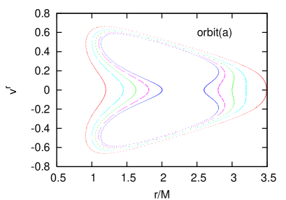
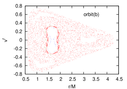
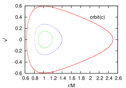
Figure 1: Poincaré maps of orbits of a particle with $H=-0.2$ and $L=1$ across the plane $z=0$ in a system of a point mass with a disk. We set the thickness the of the disk $z_{0}=0.5$, and its surface density (a) $\alpha=0.01$, (b) $\alpha=0.1$, or (c) $\alpha=10.0$. All figures are superpositions of trajectories starting from different initial conditions. In Figs. (a) and (c), all trajectories form regular tori. In Fig. (b), some trajectories from certain initial conditions still seem to form tori, but others do not. In fact, one initial condition, $(\varpi,v^{\varpi},z,v^{z})=(1.2,0,0,0.76)$ gives an almost two dimensional map on which the orbital points are widely scattered, which means that the particle motion is chaotic (We call it Orbit (b)). The outermost trajectories in Fig. (a) and (c) are called Orbit (a) and (c), whose initial conditions are $(\varpi,v^{\varpi},z,v^{z})=(1.2,0,0,0.76)$ and $(2.5,0,0,0.49)$, respectively.

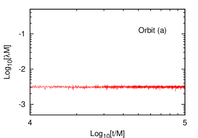
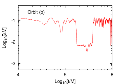
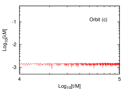
Figure 2: The time evolutions of “local” Lyapunov exponents for Orbits (a), (b), and (c) in Fig. 1. The Lyapunov exponents for Orbits (a) and (c) settle down to very small values, but that for Orbit (b) is large and changing in time. It decreases to a very small value in the time interval of $t/M=(1.6\sim 3.8)\times 10^{5}$.

We set $M=1$ to fix our units. There are two parameters of a disk which we can change, i.e., the surface density $\alpha$ and the width $z_{0}$. Which parameter dependence we should analyze ? When we change $\alpha$, there are two extreme limits, i.e., $\alpha\to 0$ and $\alpha\to\infty$, in which the system becomes integrable (see Eq. (4)). The gravity by the central mass becomes dominant when $\alpha\to 0$, while the force driven by the disk is dominant as $\alpha\to\infty$. On the other hand, if we consider two extreme limits of $z_{0}$, i.e., the limits of $z_{0}\to 0$ and of $z_{0}\to\infty$, we find that the system is still nonintegrable even in such limits  Saa:1999je . Our main aim is to make a distinction between various types of chaotic behaviours. For our purpose, the comparison of the cases with different values of $z_{0}$ may not be appropriate. Hence we analyze the cases with different values of $\alpha$, which may provide us continuous change from a regular orbit to a very strongly chaotic one.

The parameters of particle orbits such as the energy and angular momentum are appropriately chosen such that the motion is bounded. We choose the orbital parameters as $H=-0.2$ and $L=1$, and the disk width as $z_{0}=0.5$. Figure 1 shows a set of Poincaré maps for different values of the surface density ((a) $\alpha=0.01$, (b) $\alpha=0.1$, and (c) $\alpha=10.0$). The equatorial plane $(z=0)$ is chosen for a Poincaré section. We plot the points on the $(\varpi,v^{\varpi})$ plane when the particle crosses the Poincaré section with $v^{z}>0$. In these figures, trajectories starting from various initial conditions are shown. From Figs. 1 (a) and (c), we confirm these system are almost integrable. The outermost trajectories are called Orbit (a) and Orbit (c). On the other hand, a widespread chaotic sea is found in Fig. 1 (b). This is because the forces by the point mass and by the disk are comparable and those are competing each other. In Fig. 1 (b), we see the “outermost” trajectory with the initial condition of $(\varpi,v^{\varpi},z,v^{z})=(1.2,0,0,0.76)$ (called Orbit (b)) is not a simple torus but forms an almost two dimensional distribution in which the orbital points are widely scattered. It means that the particle motion is chaotic.

Figure 2 shows the time evolution of the Lyapunov exponents for Orbits (a), (b), and (c) in Fig. 1. Here we show a “local” Lyapunov exponent defined in Appendix A. We only refer to the integration time interval $t_{\Delta}$ to define it (see Appendix in more details). $t_{\Delta}$ is chosen to be $t_{\Delta}=10^{4}$, which satisfies the condition of $t_{D}\ll t_{\Delta}\ll t_{T}$ with $t_{D}(\approx 10\sim 10^{2})$ and $t_{T}(\approx 10^{6})$ being the dynamical time and the total integration period of our calculation, respectively. We also calculate it with other time intervals, $t_{\Delta}=2$ or $4\times 10^{4}$. We find that the result is not sensitive to this choice. We numerically calculate the exponents with the algorithm shown in Shimada and show the maximum component of it.

The value for Orbit (a) is very small and almost constant foot . For Orbit (c), the system is not exactly integrable. The system in the limit of $\alpha\rightarrow\infty$ is of course integrable, but there is no bound orbit in such a limit. Since we are analyzing a bound orbit, even if $\alpha$ is very large, we cannot ignore the gravitational effect of a point mass. It makes the system nonintegrable. Nevertheless, the motion looks very regular (see the Poincaré map in Fig. 1). In fact we find a very small Lyapunov exponent, which is smaller than that of Orbit (a) as shown in Fig. 2. This value is also almost constant, which means that the strength of the chaos does not change much in time. Hence we may regard this orbit as a regular one.

On the other hand Orbit (b) gives large positive Lyapunov exponent. It also shows time variation. We should note that the value quickly goes down to a very small one in the time interval of $t/M=(1.6\sim 3.8)\times 10^{5}$. We pick up the data around this interval and show the time evolution of the $r$-position of the particle and the Poincaré map in Fig. 3.

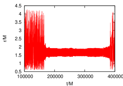
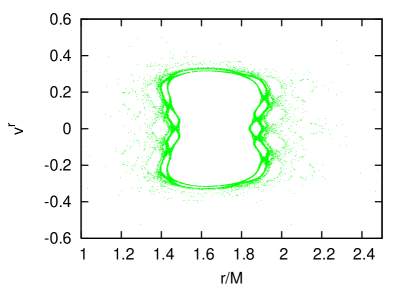
Figure 3: The particle motion in the $r$-direction in terms of time and its Poincaré map for the time interval between $t/M=10^{5}$ and $t=4\times 10^{5}$ for Orbit (b). The Poincaré map shows there exist many small tori around the origin.

From this, we find that although the particle motion in Orbit (b) is chaotic, it stays around $r\sim 1.2-2.2M$ in the time interval of $t/M=(1.6\sim 3.8)\times 10^{5}$. The motion in this period seems to be nearly regular. In fact, the “local” Lyapunov exponent decreases to $5\sim 6\times 10^{-3}$, which is almost the same as those of Orbits (a) and (c). We call this phase of motion Orbit (b-2). The phase before this interval, in which a particle motion looks very chaotic, is called Orbit (b-1). We have also performed numerical integration for longer time period and confirm such phases as Orbit (b-2) often appears in a chaotic orbit (see Fig. 4). The important point is that two different phases of motion appear and both a nearly integrable and a more strongly chaotic motion co exist in the same trajectory.

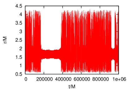
Figure 4: The particle motion of Orbit (b) in the $r$-direction for a longer time interval than that in Fig. 3. There exists new stagnant motion as the same one in Fig. 3.

The Poincaré map of Orbit (b-2) in Fig. 3 shows that many small tori exist. It is well known that such a structure appears if an orbit is nearly integrable and produces the so-called $1/f$ fluctuation  Karney:1995 ; Contopoulos:2000 ; Contopoulos:2002 ; Koyama:2007cj . Then we also analyze the power spectrum of the $r$-component of Orbit (b-2), which clearly shows a $1/f$ fluctuation for $f\leq 10^{-2}M^{-1}$ (see Fig. 5). This confirms our previous result Koyama:2007cj in the present model.

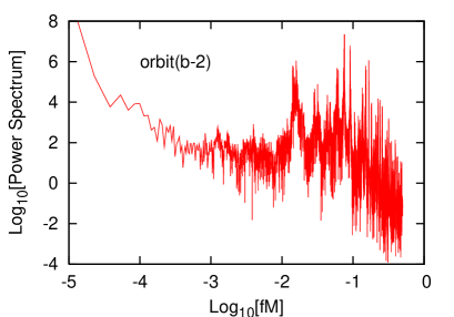
Figure 5: The power spectrum of the motion in the $r$-direction of Orbit (b-2), which is part of nearly regular motion in Orbit (b) ( $t/M=(1.6\sim 3.8)\times 10^{5}$). We find a power-law spectrum, e.g., a $1/f$ fluctuation. This is a reflects the existence of small tori in the phase space, and the particle moves almost regularly there Koyama:2007cj .

III.2 Indication of chaos in gravitational waves

Next we study how to extract information from such a chaotic system and distinguish the orbits, i.e., a nearly integrable and more strongly chaotic motions.

In Koyama:2007cj , the authors focused on the power spectrum of particle motion moving in Schwarzschild spacetime and found that it shows a power-law behaviour. In this work, we use a similar analysis for the gravitational waves emitted from our system. It could be a new and robust way to observe chaotic behaviors in astrophysical objects, as mentioned in our Introduction. The gravitational waves from the present system are calculated by the quadrupole formula Landau , which is given by

$$h_{+}=\left[\left(h^{Q}_{xx}-h^{Q}_{yy}\right)\cos 2\varphi+2h^{Q}_{xy}\sin 2\varphi\right]\frac{(\cos^{2}\theta+1)}{4}-\left(h^{Q}_{xx}+h^{Q}_{yy}-2h^{Q}_{zz}\right)\frac{\sin^{2}\theta}{4}$$

$$~{}~{}~{}~{}~{}~{}-\left(h^{Q}_{xz}\cos\varphi+h^{Q}_{yz}\sin\varphi\right)\sin\theta\cos\theta\,,$$ (5)

$$h_{\times}=\left[2h^{Q}_{xy}\cos 2\varphi-(h^{Q}_{xx}-h^{Q}_{yy})\sin 2\varphi\right]\frac{\cos\theta}{2}+\left(h^{Q}_{xz}\sin\varphi-h^{Q}_{yz}\cos\varphi\right)\sin\theta,$$ (6)

where

$$h_{ij}^{Q}\equiv\frac{2}{r}\frac{d^{2}Q_{ij}}{dt^{2}}~{}~{}~{}~{}{\rm with}~{}~{}Q_{ij}\equiv\mu\left(Z^{i}Z^{j}-\frac{1}{3}\delta_{ij}~{}\!\!\!\mbox{ \boldmath$Z$}^{2}\right)~{}~{}({\rm the~{}reduced~{}quadrupole~{}moment~{}of~{}a~{}point~{}mass}).$$ (7)

$(r,\theta,\varphi)$ [or $(x,y,z)$] is the position of a distant observer in spherical coordinates [or Cartesian coordinates], and $\!\!\!\mbox{ \boldmath$Z$}(t)$ is a trajectory of a particle. We assume that the observer is on the equatorial plane, i.e. $(\theta,\varphi)=(\pi/2,0)$. Figure 6 shows the waveforms from Orbits (a), (b), and (c). The left panels show the “$+$” polarization modes of those waves, while the right ones are the “$\times$” polarization. The top, middle, and bottom panels correspond to the waves from Orbits (a), (b), and (c), respectively. The waves from Orbits (a) and (c) show a periodic feature, which is expected from the Poincaré maps in Fig. 1. On the other hand, the waves from Orbit (b) show a completely different behaviour. We find much random spiky noise in the waveform before $t/M=1.6\times 10^{5}$ and after $t/M=3.8\times 10^{5}$. This is a typical feature of the gravitational waves from highly chaotic motion Kiuchi:2004bv ; Suzuki . We also find that the amplitude decreases for the time interval of $t/M=(1.6\sim 3.8)\times 10^{5}$. As shown in Fig. 3, in this time interval, the particle moves near the small tori in the phase space. This adjective feature of this particle motion appears clearly in the gravitational amplitudes. That is, in the phase of a nearly regular motion, the particle position and its velocity do not change much compared with those in the more strongly chaotic phase (b-1) (see Fig. 1(b) and Fig. 3(b)). The time variation of the quadrupole moment of the system is small and hence the wave amplitude decreases as well.

We also calculate the energy spectra of the gravitational waves, which will be one of the most important observable quantities in the near future. In Fig. 7, we show the energy spectra for each orbit. Figures 7(a) and (c) show many sharp peaks at certain characteristic frequencies. If a motion is regular, we expect several typical frequencies with those harmonics. So such a result reflects that the particle moves regularly. Figure 7 (b) gives the spectrum of Orbit (b). It is clearly different from the previous two almost regular cases. It looks just like white noise, below a typical frequency $fM\sim 10^{-2}$, i.e., the shape of the spectrum is flat and it contains many noisy components. However, the spectrum of Orbit (b-2) (Fig. 7(b-2)), which is analyzed by the orbit only in the time interval of $t/M=(1.6\sim 3.8)\times 10^{5}$, does not do so. Rather it looks similar to the spectrum of a regular orbit. Contrary to Fig. 7(b), it does not contain much noise at the low frequency region ($fM\leq 10^{-2}$).

To see more detail, dividing the time interval of Orbit (b) into two, we show the magnifications of the spectra of Orbits (a), (b-1), (b-2), and (c) in Fig. 8. Compared to the spectra (a) and (c), the spectra (b-1) and (b-2) contain many noisy spikes. Such noisy spikes are usually found in the gravitational waves from a chaotic orbit Kiuchi:2004bv . However, the spectra (b-1) and (b-2) are completely different. The spectrum (b-1) is just white noise. No structure is found. On the other hand, the spectrum (b-2) looks similar to those for regular orbits. The “sharp” peaks appear at some frequencies, but the widths of those peaks are broadened by many noisy spikes. Therefore, we conclude that Orbit (b-2) looks nearly regular but still holds its chaotic character, and such a feature imprints in the spectrum of the waves. The important point is that two phases in the particle orbit (b), i.e., the nearly regular phase and the more strongly chaotic one, are also distinguishable in the gravitational wave forms and the energy spectra. With this analysis, we could constrain orbital parameters.

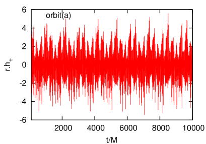
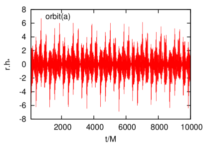
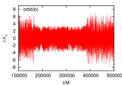
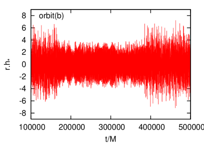
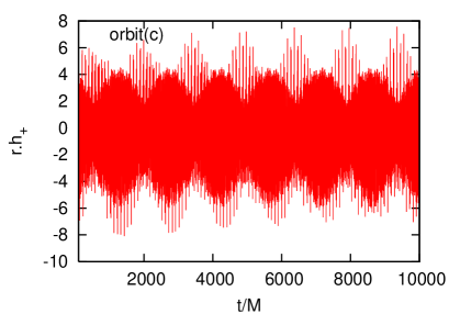
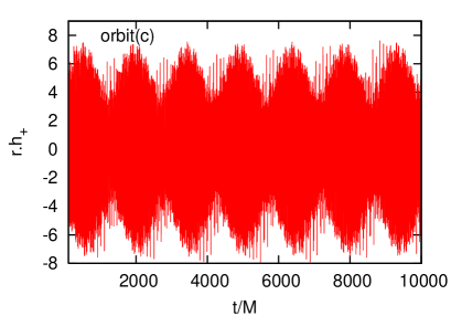
Figure 6: The gravitational waveforms evaluated by the quadrupole formula. Top, middle, and bottom figures correspond to those for Orbits (a), (b), and (c), respectively. The left and right rows give the “$+$” and “$\times$” polarization modes, respectively.

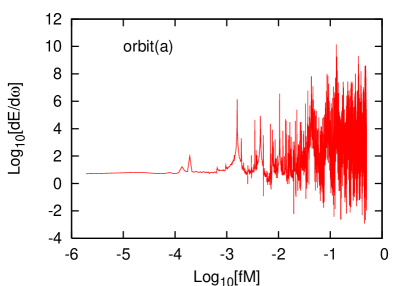
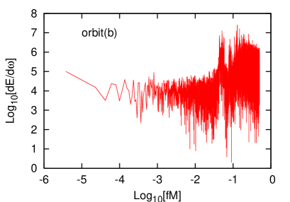
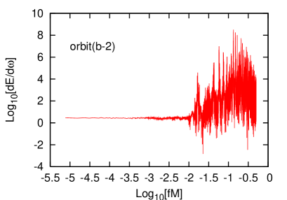
Figure 7: The energy spectra of the gravitational waves shown in Fig. 6. Orbit (b-2) gives the spectrum of the waves for the “stagnant motion”, i.e., when the particle motion of Orbit (b) becomes near regular for $t/M=(1.6\sim 3.8)\times 10^{5}$. Figures (a) and (c) show many sharp peaks at certain characteristic frequencies. This is because of the regular motion. The spectrum in Fig. (b), which looks like white noise for $fM\leq 10^{-2}$, is clearly different from those in Figs. (a) and (c), but the spectrum in Fig. (b-2) does not look like white noise. It looks similar to the cases (a) and (c). However, the peaks are not sharp but rather broadened by appearing so many other spikes. Note that the typical frequency of the orbits is in the range of $fM=10^{-2}\sim 10^{-1}$ (see Fig. 5).

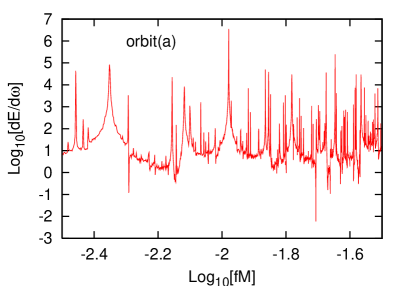
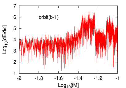
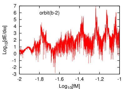
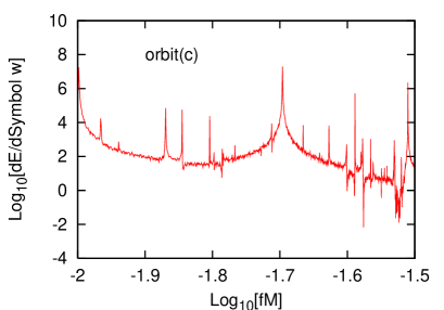
Figure 8: Magnification of energy spectra of Orbits (a), (b-1), (b-2), and (c).

IV Summary and Discussion

In this paper we have investigated chaos characteristic for a test particle motion in a system of a point mass with a massive disk in Newtonian gravity. To distinguish such characteristics, we propose the gravitational waves emitted from this system. At first, we analyzed the motion of the particle by use of the Poincaré map and the “local” Lyapunov exponent. We found that the phase in which particle motion becomes nearly regular always appears even though the global motion is chaotic. We emphasize that both phases of nearly regular and more strongly chaotic motions are found in the same orbit.

The gravitational wave forms and their energy spectra have been evaluated by use of the quadrupole formula in each case. In two almost regular cases, the waves show the periodic behaviour and certain sharp peaks appear in those energy spectra. In the chaotic case, we have found that the waves show two phases, the nearly regular phase and a more strongly chaotic one. In the nearly regular phase, wave amplitude gets smaller in the more strongly chaotic phase. The energy spectra are also clearly different. The spectrum in the more strongly chaotic phase looks like white noise, but in the nearly regular one, it becomes similar to those in the regular ones. However it is accompanied by many small noisy spikes, which is a characteristic feature of a chaotic system. These spikes make the widths of the spectrum peaks broader than those in the regular cases. Comparing information from the waves with the particle motion, we conclude that we can extract chaotic characteristics of a particle motion of the gravitational waves of the system. In the present analysis, in the spectrum (b-2) of the gravitational waves, we do not find a power-law structure, which appears in the spectrum of the particle motion. This may be because the waveform is given by the change of the quadrupole moment, which contains higher time derivatives of a particle trajectory such as acceleration. It may be much more interesting if one can find the $1/f$ behaviour in some information of the gravitational waves because such an indication may specify the type of chaos more clearly. This is under investigation.

Finally, we mention a possibility to constrain parameters in a dynamical system. If the gravitational waves are observed for a sufficiently long time, we can monitor the time variation of the wave amplitudes, their forms and polarizations. We can then calculate the energy spectra for some durations. If the spectra show one of the typical characteristics found in this paper, the parameters of a particle motion could be constrained. Of course, a realistic system can be more complicated, and the present model may be too simple. But we believe the characteristic behaviour of the gravitational waves found in this paper will help us to understand a chaotic system. Therefore our next task is to analyze the gravitational waves from various chaotic systems, especially relativistic chaotic systems Lemos:1993qp ; Karas ; Varvoglis ; Bombelli ; Moeckel ; Yust ; Sota ; Suzuki ; letelier_viera ; podolsky_vesely ; Kiuchi:2004bv ; Koyama:2007cj . Then, we should investigate whether or not the correlation between the gravitational waves and chaos in dynamical systems found in this work is generic.

Appendix A Local Lyapunov Exponent

In this appendix, we give the definition of “local” Lyapunov exponent. Our definition of “local” Lyapunov exponent is somewhat different from the conventional oneLLE , but those are essentially the same.

At first, let us consider the system whose time evolution is described by a set of differential equations in $N$-dimensional space,

$$\dot{{\bf x}}={\bf F}({\bf x})\,,$$ (8)

where ${\bf x}(t)$ is a $N$-dimensional vector.

The time evolution of the orbital deviation $\delta{\bf x}$, which is the difference between two nearby orbits, obeys the following set of linear differential equations:

$$\delta\dot{{\bf x}}=\frac{\partial{\bf F}}{\partial{\bf x}}({{\bf x}(t)})\delta{\bf x}.$$ (9)

The solution of Eq. (9) can be written formally as

$$\delta{\bf x}(t)=U^{t}_{~{}t_{0}}\delta{\bf x}_{0},$$ (10)

where $\delta{\bf x}_{0}$ is an “initial” deviation at some time $t_{0}$ and $U^{t}_{~{}t_{0}}$ is an evolution matrix, which is given by the following integration;

$$U^{t}_{~{}t_{0}}=\exp\left[\int^{t}_{t_{0}}\frac{\partial{\bf F}}{\partial{\bf x}}({{\bf x}(t^{\prime})})dt^{\prime}\right]\,.$$ (11)

We define the “local” Lyapunov exponent in time interval $[t_{0},t]$ by

$$\lambda(e^{k},t)=\frac{1}{t-t_{0}}\log\frac{||U^{t}_{~{}t_{0}}{\bf e}_{1}\wedge U^{t}_{~{}t_{0}}{\bf e}_{2}\wedge\cdots\wedge U^{t}_{~{}t_{0}}{\bf e}_{k}||}{||{\bf e}_{1}\wedge{\bf e}_{2}\cdots\wedge{\bf e}_{k}||}$$ (12)

for $k=1,2,\cdots,N$, where $e^{k}$ is a $k$-dimensional subspace in the tangent space at the initial point ${\bf x}_{0}$, which is spanned by $k$ independent vectors ${{\bf e}_{i}}$ $(i=1,2,\cdots,k)$, $\wedge$ is an exterior product, and $||\circ||$ is a norm with respect to some appropriate Riemannian metric. If we take a limit of $t\rightarrow\infty$, $\lambda(e^{k},\infty)$ correspond to the conventional Lyapunov exponents.

If the integration time interval $t_{\Delta}\equiv t-t_{0}$ is much longer than the dynamical time of the system, we may find convergent values for each $\lambda(e^{k},t)$, which are almost independent of $t_{\Delta}$ (or $t_{0}$). We may call them “local” Lyapunov exponents at $t$. The maximum value of “local” Lyapunov exponents, i.e. $\lambda(t)=\max\{\lambda(e^{k},t)|k=1,2,\cdots,N\}$ is the most important one for our discussion. So we also call it the “local” Lyapunov exponent at $t$.

References

- (1) Deterministic Chaos in General Relativity, edited by D. Hobill, A. Burd, and A. Coley (Plenum, New York, 1994), and references therein.
- (2) J.D. Barrow, Phys. Rep. 85, 1 (1982).
- (3) G. Contopoulos, Proc. R. Soc. London A431,183(1990).
- (4) V. Karas and D. Vokrouhlický, Gen. Rela. Grav. 24,729(1992).
- (5) H. Varvoglis and D. Papadopoulos, Astron. Astrophys. 261,664(1992).
- (6) L. Bombelli and E. Calzetta, Class. Quantum Grav. 9,2573(1992).
- (7) R. Moeckel, Commun. Math. Phys. 150,415(1992).
- (8) C.P. Dettmann, N.E. Frankel and N.J. Cornish, Phys. Rev. D 50, 618(1994).
- (9) U. Yurtsever, Phys. Rev. D 52,3176(1995).
- (10) Y. Sota, S. Suzuki, and K. Maeda, Class. Quantum Grav. 13,1241(1996).
- (11) S. Suzuki and K. Maeda, Phys. Rev. D 55,4848(1997); 58,023005(1998); 61,024005(1999).
- (12) P.S. Letelier and W.M. Viera, Phys. Rev. D 56,8095(1997).
- (13) J. Podolsky and K. Vesely, Phys. Rev. D 58, 081501(1998).
- (14) J. Levin, Phys. Rev. Lett. 84,3515(2000).
- (15) J.D. Schnittman and F.A. Rasio, Phys. Rev. Lett. 87, 121101 (2001).
- (16) N.J. Cornish and J. Levin, Phys. Rev. Lett. 89,179001(2002).
- (17) K. Kiuchi and K. Maeda, Phys. Rev. D 70,064036(2004)
- (18) C.F.F. Karney, Physica D 8,360(1983)
- (19) G. Contopoulos, M. Harsoula and N. Voglis, Celest. Mech. Dyn. Astron. 78,197(2000)
- (20) G. Contopoulos, Order and Chaos in Dynamical Astronomy, (Springer, 2002)
- (21) H. Koyama, K. Kiuchi and T. Konishi, arXiv:gr-qc/0702072.
- (22) K. Tsubono, Prepared for Edoardo Amaldi Meeting on Gravitational Wave Experiments, Rome, Italy, 14-17 Jun 1994
- (23) A. Abramovici et al., “LIGO: The Laser interferometer gravitational wave observatory,” Science 256, 325 (1992).
- (24) J. Hough et al., Prepared for TAMA Workshop on Gravitational Wave Detection, Saitama, Japan, 12-14 Nov 1996
- (25) K.S. Thorne, arXiv:gr-qc/9506086.
- (26) A. Saa and R. Venegeroles, Phys. Lett. A 259,201(1999)
- (27) A. Saa, Phys. Lett. A 269,204(2000)
-
(28)
The recent observation suggests there exist huge black holes
at the centers of many galaxies.
See, for example,
J. Kormendy and D. Richstone, Astrophys. J. 393,559(1992) - (29) I. Shimada and T. Nagashima, PTP 61, 1605 (1979)
- (30) The reason why we find non-zero positive Lyapunov exponent for an integrable system is that we solve the equation of motion by a finite difference method and the finite difference approximation does not provide an exact integrable system. In fact, if we reduce the time step for integration, the value decreases.
- (31) W.C.Saslaw, Gravitational physics of stellar and galactic systems, Cambridge University Press, 1985.
- (32) J.P.S. Lemos and P.S. Letelier, Phys. Rev. D 49,5135(1994).
- (33) L. D. Landau and E. M. Lifshitz, The Classical Theory of Fields, (Pergamon, Oxford, 1951).
- (34) P. Grassberger, R. Badii, and A. Politi, J. Stat. Phys. 51, 135 (1988); H. E. Kandrup, B. L. Eckstein, and B. O. Bradley, Astron. Asrophys. 320, 65 (1997)