Flavor Composition and Energy Spectrum of Astrophysical Neutrinos

Abstract

The measurement of the flavor composition of the neutrino fluxes from astrophysical sources has been proposed as a method to study not only the nature of their emission mechanisms, but also the neutrino fundamental properties. It is however problematic to reconcile these two goals, since a sufficiently accurate understanding of the neutrino fluxes at the source is needed to extract information about the physics of neutrino propagation. In this work we discuss critically the expectations for the flavor composition and energy spectrum from different types of astrophysical sources, and comment on the theoretical uncertainties connected to our limited knowledge of their structure.

I Introduction

There is the expectation that in the near future we will see the opening of the new field of observational high energy neutrino astronomy nuh ; nuh1 ; lip-catania . Theoretically there are very robust reasons to expect the existence of high energy ($E_{\nu}\gtrsim 10^{12}$ eV) neutrino sources. The strongest motivation is the observation of a cosmic ray flux, mostly composed of protons and fully ionized nuclei that extends in energy up to $E\sim 10^{20}$ eV. These hadronic particles can interact inside or near their acceleration sites or during their propagation in interstellar or intergalactic space. These interactions produce weakly decaying particles (such as $\pi^{\pm}$ and kaons) that generate neutrinos. These “astrophysical neutrinos” are intimately connected with the high energy photons that are created in the decay of $\pi^{\circ}$ and $\eta$ particles produced in the same hadronic primaries interactions, or in the radiation processes of relativistic electrons and positrons co–accelerated in the sources. A rich variety of high energy gamma ray sources has been observed with detectors on satellites egret-3rd and ground–based hess-scan Cherenkov telescopes, suggesting several possible neutrino sources.

Observations with neutrinos have the potential to give us unique information about their astrophysical sources, and hopefully could also result in the discovery of new classes of sources. On the other hand the possibility to use these observations to obtain information about the fundamental properties of the neutrinos has been widely discussed nuh ; double-bang ; Athar:2000yw ; Ahluwalia:2001xc ; Pakvasa:2004hu ; Barenboim:2003jm ; Beacom-flavor . Astrophysical neutrinos travel pathlengths of order $10$ Kpc ($\sim 3\times 10^{22}$ cm) for galactic sources, and as large as $\sim 1$ Gpc ($\sim 3\times 10^{27}$ cm) for extragalactic sources. These remarkably long baselines allow the study of phenomena such as $\nu$ flavor transitions or $\nu$ decay in a range of parameters that is unaccessible with other methods. Only observations with SuperNova neutrinos, very likely only observable from galactic sources, but having much smaller energy ($E_{\nu}\sim 10$ MeV) could provide larger $L/E_{\nu}$.

In order to extract information about the neutrino fundamental properties from the observations one needs to have sufficiently good understanding of the properties of the neutrino emission at the source. The common assumption in several studies of this type is that the properties of the $\nu$ emission, and in particular the flavor composition at the source can be robustly predicted. There is of course a well known historical precedent for the successful use of this concept in the discovery of neutrino oscillations with atmospheric neutrinos. In fact, the first hints of the existence of the now solidly established $\nu_{\mu}\leftrightarrow\nu_{\tau}$ transitions were obtained with the Kamiokande Kamiokande and IMB IMB detectors as the measurement of a $\mu/e$ ratio for contained events smaller than the expectations. It is natural to try to make use of new, very distant neutrino sources (when they will be discovered) to perform additional studies of the properties of neutrino propagation.

Several “exotic” processes, beyond standard flavor oscillations, could reveal themselves only in the propagation of neutrinos over very long distances. For example, it has been suggested that some neutrinos could decay into a lighter neutrino and a majoron majoron , if the lifetime is sufficiently long this phenomenon could be only detectable for neutrinos propagating over astronomical distances Acker:1991ej ; nu-decay . A second interesting possibility is that neutrinos are pseudo–Dirac states pseudoDirac where each generation is actually composed of two maximally-mixed Majorana neutrinos separated by a tiny mass difference. If the pseudo-Dirac splittings are sufficiently small, the phenomenology of oscillations on short baselines remains unchanged, however when $E_{\nu}/L$ becomes comparable or smaller than the pseudo–Dirac splittings new transitions become possible, and can in principle be detectable with astrophysical neutrinos beacom-pd . More in general, oscillations into sterile states that are quasi degenerate to the active neutrinos can in principle be investigated down to very small squared mass splittings steriles . Several other mechanisms such as quantum decoherence Hooper:2004xr , violations of the equivalence principle Gasperini:1989rt ; Minakata:1996nd , neutrinos with varying masses Fardon:2003eh ; Hung:2003jb could leave their signature on the propagation of astrophysical neutrinos.

A well known “naive” argument states that since the dominant source of astrophysical neutrinos is the decay of charged pions, and each $\pi^{\pm}$, after chain decays such as: $\pi^{+}\to\mu^{+}\nu_{\mu}\to(\overline{\nu}_{\mu}\,e^{+}\,\nu_{e})\,\nu_{\mu}$, generates two muon neutrinos and one electron neutrino, the flavor ratio at the source is $R_{\mu e}=(\nu_{\mu}+\overline{\nu}_{\mu})/(\nu_{e}+\overline{\nu}_{e})\simeq 2$. This naive argument has some pedagogical value, but must be considered only as a first approximation. In fact, even if charged pions are the only source of neutrinos, $R_{\mu e}$ is only equal to 2 after integration over all $\nu$ energies, because the three neutrinos generated in a charged pion decay have different energy spectra, and therefore in general the flavor ratio will depend on the spectral shape of the $\nu$ signal, and will vary with the neutrino energy. An effect that can be of large importance is the presence of sufficiently efficient energy loss mechanisms in the source. In this situation the particles that are most affected are the muons. The presence of additional neutrino sources (such as kaons) can also be important for the flavor ratio. In this work we will re–examine critically the uncertainties in the predictions of the spectra and flavor composition of astrophysical neutrinos and discuss the implications for the extraction of information on the neutrino properties.

This paper is organized as follows: in the next section we discuss how the observable neutrino flavor ratios carry information at the same time about the flavor composition at the source and about the flavor transition probabilities. In section 3 we outline the general structure of the calculation of the neutrino signal from an astrophysical source. The different steps of these calculations are considered in more details in sections 4–7. In section 8, as an illustration, we describe an explicit calculation of the neutrino emission from the fireballs of Gamma Ray Bursts following the model of Waxman and Bahcall Waxman-grb . Section 9 contains a short discussion of the problem of the experimental determination of the flavor composition and energy spectra of a neutrino signal. The last section presents our conclusions.

II Flavor Ratios of Astrophysical Neutrinos

The observable fluxes of astrophysical neutrinos from a source at distance $L$ will be linear combinations of the fluxes at the source. Leaving implicit the energy and distance dependences one can write:

$$\phi_{\nu_{\alpha}}=\sum_{\nu_{\beta}}P_{\nu_{\beta}\to\nu_{\alpha}}~{}\phi_{\nu_{\beta}}^{\circ}~{}~{}.$$ (1)

The transition probabilities $P_{\nu_{\beta}\to\nu_{\alpha}}$ have certainly a non trivial structure because of the known existence of “standard” flavor oscillations, but might depend on additional “new physics” contributions, such as neutrino decay, that become significant only for very long pathlengths. In the standard scenario the neutrino number is conserved and therefore $\sum_{\beta}P_{\alpha\to\beta}=1$. More in general, in the presence of a non negligible decay probability or of transitions to additional sterile states, the sum can be less than unity.

The flavor, energy and pathlength dependences of the standard oscillation probabilities are well known, and are determined by two squared mass differences ($\Delta m^{2}_{12}\simeq 8.0\times 10^{-5}$ eV², $|\Delta m^{2}_{23}|\simeq 2.5\times 10^{-3}$ eV²) and the neutrino mixing matrix. The oscillation lengths ($\lambda_{ij}=4\pi\,E_{\nu}/|\Delta m^{2}_{ij}|$) of the standard flavor transitions are short with respect to the typical astrophysical distances and, in most cases, it is a good approximation to consider only the probability averaged over distance. In this case the probability becomes independent from $E_{\nu}$ and $L$ and takes the form:

$$\langle P_{\nu_{\alpha}\to\nu_{\beta}}^{\rm standard}\rangle_{L}=\sum_{j}|U_{\alpha j}|^{2}\,|U_{\beta j}|^{2}$$ (2)

where $U$ is the unitary mixing matrix that relates the neutrino flavor and mass eigenstates. This matrix can be written in terms of three mixing angles and one CP violating phase. From a global fit to all existing neutrino data Strumia:2005tc one can extract the best fit values: $\theta_{12}\simeq 34^{\circ}$, $\theta_{23}\simeq 45^{\circ}$, $\theta_{13}\simeq 0$, and 99% C.L. intervals for the mixing angles: $\theta_{12}\in[30^{\circ},38^{\circ}]$, $\theta_{23}\in[36^{\circ},54^{\circ}]$, $\theta_{13}\leq 10^{\circ}$; the phase $\delta$ remains completely undetermined.

Assuming to know sufficiently well the properties of the source, the observed flavor ratios can give information on the flavor transition probabilities. This can be used to help in the determination of the “standard” parameters in the flavor oscillations, or more ambitiously to investigate the possible existence of additional phenomena in neutrino propagation.

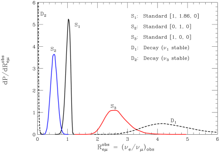
Figure 1: Distribution of the observable flavor ratio $R_{e\mu}=(\nu_{e}/\nu_{\mu})_{\rm obs}$ for different models of the $\nu$ source and different neutrino properties. A source model is defined by the relative intensity (summing over $\nu$ and $\overline{\nu}$) of the emission for the three flavors: [$\nu_{e},\nu_{\mu},\nu_{\tau}]_{\rm source}$. The distribution of $R_{e\mu}$ is entirely due to the present uncertainties in the determination of the $\nu$ mixing parameters. The source models $[0,1,0]$, and $[1,0,0]$ correspond to pure $\nu_{\mu}$ or $\nu_{e}$ emission; the model $[1,1.86,0]$ corresponds to the pion dominated emission from a thin source with a power law spectrum of slope 2. The two dashed curves show the distributions of $R_{e\mu}$ for a $\nu$–decay model nu-decay where only the lowest $\nu$ mass eigenstate (in the direct and inverse hierarchy) is stable.

As an illustration in fig. 1 and 2 we show the expectations for the two independent flavor ratios $R_{e\mu}=(\nu_{e}/\nu_{\mu})_{\rm obs}$ and $R_{\mu\tau}=(\nu_{\mu}/\nu_{\tau})_{\rm obs}$, calculated for different assumptions for the source emission, in the presence of simple standard oscillations, or also including neutrino decay (with two different assumptions) nu-decay . The distributions of the flavor ratio for a given model are determined only by the present uncertainties on the neutrino mixing parameters. A source model is defined by the relative intensity of the emission for the three neutrino flavors. For our illustration we have considered three source models. The first model is the emission of form: [$\nu_{e},\nu_{\mu},\nu_{\tau}]_{\rm source}=[1,1.86,0]$. This corresponds (as we will discuss more extensively in the following) to pion dominated emission from a thin source (no significant energy loss for secondaries) with a power law energy spectrum of slope 2. Several classes of $\nu$ sources of this type (such as Supernova Remnants and Gamma Ray Bursts) have been predicted. Note that the flavor relative abundances in this model are close but not identical to the naive expectation [1,2,0]. The deviations are a simple consequence of the shape of the energy spectra of the neutrinos in pion chain decay. The observable $R_{e\mu}$ ratio for this model takes value in the interval $\simeq(0.7,1.2)$ with a most likely value close to unity, while the other independent ratio $R_{\mu\tau}$ has a narrow distribution sharply peaked at the value 1, with a tail extending up to $\simeq 1.3$.

Figures 1 and 2 also show the predicted flavor ratios for emission with (summing over $\nu$ and $\overline{\nu}$) flavor abundances $[0,1,0]$, and $[1,0,0]$, that is pure muon or electron neutrino emission. The motivation for using these two models is that, to a very good approximation, they can be considered the two extreme models for the emission from a “standard” (not involving new physics) source, since a significant production of $\nu_{\tau}$ in an astrophysical environment is extraordinary unlikely. Sources emitting pure fluxes of $\nu_{\mu}$ or $\nu_{e}$ are in principle possible, and have been in fact advocated in the literature. They correspond to a source dominated by pions where muons lose all their energy before decay, or to a pure neutron source, that generates a $\overline{\nu}_{e}$ flux. A pure neutron ($\overline{\nu}_{e}$) neutrino source is in fact unrealistic since it is natural that neutron production is associated with pion production and therefore with some $\nu_{\mu}$ emission. We will comment more extensively on these issues in the following.

For the [0,1,0] ([1,0,0]) model the most likely value for the observable flavor ratio is $R_{e\mu}\simeq 0.55$ ($R_{e\mu}\simeq 2.7$). In both cases $R_{\mu\tau}$ is centered at the value unity, this is a simple consequence of the large (approximately maximal) mixing between $\nu_{\mu}$ and $\nu_{\tau}$. In the case of a [1,0,0] source the $R_{\mu\tau}$ distribution is noticeably broader extending to the interval $R_{\mu\tau}\in(0.5,1.5)$.

Neutrino decay with a very long lifetime is one of the most interesting possibilities that can be investigated with astrophysical neutrinos. Assuming nu-decay ; Barenboim:2003jm that only the lowest mass eigenstate is stable, and that the distance of the source is much longer than the decay lengths, the observable flavor ratios depend uniquely on the flavor composition of the lightest eigenstate. Depending on the sign of $\Delta m^{2}_{23}$ this is $\nu_{1}$ (direct mass hierarchy) or $\nu_{3}$ (inverse hierarchy). The flavor ratios for these two models are also shown in fig. 1 and 2 as dashed lines. The $R_{e\mu}$ ratio is particularly interesting. In the case of direct mass hierarchy, the most probable value of the $e\mu$ ratio is large ($R_{e\mu}\simeq 4.2$), the distribution is also remarkably wide, allowing in principle to constrain the mixing parameters nu-decay . For the inverse hierarchy, when the stable neutrino is the $\nu_{3}$ that has a small (or perhaps vanishing) overlap with $\nu_{e}$, the observable $R_{e\mu}$ is close to zero.

It is remarkable that the predictions for the $e\mu$ flavor ratio in neutrino decay are in both (direct and inverse mass hierarchy) models significantly different from the standard model predictions for nearly all assumptions about the flavor composition of the emission. Only a pure $\nu_{e}$ emission has some overlap with the decay model with stable $\nu_{1}$. The study of the $e\mu$ flavor ratio of astrophysical neutrinos can therefore give evidence in favor or against the existence of $\nu$ decay.

The determination of the neutrino mixing parameters in the standard oscillation scenario is more problematic. For the most sensitive $e\mu$ ratio, the range of possible values due to the present uncertainties on the mixing parameters is in fact smaller than the variations that result from different flavor abundances at the source. Therefore the possibility to obtain interesting bounds on the mixing parameters depends crucially on having a sufficiently precise knowledge of the source.

To illustrate this problem, we can write an approximate expression for the flavor ratio $R_{e\mu}$ in terms of the relevant mixing matrix parameters expanding in first order around the best fit values

$$\left(\frac{\nu_{e}}{\nu_{\mu}}\right)_{\rm obs}^{[1,1.86,0]}\simeq 1.026-0.0218~{}\delta\theta_{23}^{\circ}+0.0087~{}\theta_{13}^{\circ}\;\cos\delta-0.0014~{}\delta\theta_{12}^{\circ}+0.370~{}\delta\left(\frac{\nu_{e}}{\nu_{\mu}}\right)_{0}~{}~{}~{}$$ (3)

$$\left(\frac{\nu_{e}}{\nu_{\mu}}\right)_{\rm obs}^{[0,1,0]}\simeq 0.547-0.0296~{}\delta\theta_{23}^{\circ}+0.0119~{}\theta_{13}^{\circ}\;\cos\delta+0.0197~{}\delta\theta_{12}^{\circ}+1.152~{}\delta\left(\frac{\nu_{e}}{\nu_{\mu}}\right)_{0}~{}~{}~{}$$ (4)

$$\left(\frac{\nu_{e}}{\nu_{\mu}}\right)_{\rm obs}^{[1,0,0]}\simeq 2.65+0.093~{}\delta\theta_{23}^{\circ}-0.037~{}\theta_{13}^{\circ}\;\cos\delta-0.131~{}\delta\theta_{12}^{\circ}-3.846~{}\delta\left(\frac{\nu_{\mu}}{\nu_{e}}\right)_{0}~{}~{}~{}$$ (5)

In these equations $\delta\theta_{12}^{\circ}$ and $\delta\theta_{23}^{\circ}$ are the deviations in degrees of the mixing angles from their best fit value ($\theta_{12}=34^{\circ}$, $\theta_{23}=45^{\circ}$), $\theta_{13}^{\circ}$ is the value (always in degrees) of the third angle and $\delta$ is the CP violating phase. The superscript labels of the flavor ratio indicate the source model. The last term in equations (3), (4) and (5) gives an estimate of the variation in the observable ratio due to the uncertainty in the flavor ratio at the source obtained expanding in first order in $\delta(\nu_{\alpha}/\nu_{\beta})_{0}$ around the flavor abundances of the model considered. One can see that uncertainties in flavor abundances at the source can be so large to make impossible a meaningful constraint on the mixing parameters.

In the remaining sections of this paper we will discuss how the properties of the astrophysical sources determine the flavor abundances of their emission, and estimate the associated theoretical uncertainties.

III Production of Astrophysical Neutrinos

Astrophysical neutrinos are generated when a population of relativistic hadrons (protons or nuclei) interacts with some target material (gas or a radiation field) inside, near, or outside the acceleration site. These interactions produce weakly decaying secondary particles whose decay generate neutrinos either directly, or indirectly with the subsequent decay of muons. The description of these processes therefore requires the following elements:

1. The description of the energy spectrum and composition of the primary particles.

2. The definition of the target material with which the primary particles interact.

3. The modeling of the properties of particle production in hadronic interactions.

4. The description of the properties of the medium where the interactions are taking place, to determine the relevant mechanisms for energy loss.

5. The (well known) properties of weak decays.

In our discussion we will describe the source as one stationary homogeneous region. This is an important limitation, because in general we can expect that the sources will have non trivial space structures, with the neutrinos emerging from different regions that can produce different spectral shapes and flavor contents; most high energy radiation sources are also expected to show important time variabilities. Because of the limited statistics and angular resolution, the observations of astrophysical neutrinos will necessarily integrate over the entire volume of the source (that in most cases will appear as point–like) and average over most or all time variations. Describing this situation requires the averaging over different source regions and conditions.

Some of the most interesting postulated sources of neutrinos, in particular the jets of Active Galactic Nuclei (AGN) and Gamma Ray Bursts (GRB), are expected to be associated with astrophysical jets with ultra–relativistic bulk motion. These relativistically moving sources are best described in the rest frame of the jet, where the emitted radiation is approximately isotropic, and the electromagnetic fields can be described as a purely magnetic field. The observable fluxes can then be obtained by an appropriate Lorentz boost.

The $\nu$ emission from a given source can be described by the emissivities $Q_{\nu_{\alpha}}(E_{\nu},\Omega)$ (in units (s sr GeV)^-1) that give the number of neutrinos of type $\alpha$ emitted with energy $E_{\nu}$ in the direction $\Omega$. The $\nu$ fluxes at the Earth are obtained from the neutrino emissivities as:

$$\phi_{\nu_{\alpha}}(E_{\nu})=\frac{(1+z)^{2}}{4\pi d_{L}^{2}}~{}\sum_{\nu_{\beta}}P_{\nu_{\beta}\to\nu_{\alpha}}(E_{\nu})~{}Q_{\nu_{\beta}}[E_{\nu}(1+z),\Omega_{\oplus}]$$ (6)

where $d_{L}$ is the source luminosity distance, $z$ is its redshift, and $P_{\nu_{\beta}\to\nu_{\alpha}}$ are the flavor transition probabilities. The observable fluxes depend only on the emission in the direction $\Omega_{\oplus}$ that corresponds to the line of sight from the source to the Earth. In the following we will not consider the angular dependence of the source emission, since this is not observable for any individual source.

The calculation of the neutrino emissivities $Q_{\nu_{\alpha}}(E_{\nu})$, starts from a decription of the energy spectrum and composition of the primary particles. In the following we will assume that the primary particles are protons and are described by the energy spectrum $N_{p}(E_{p})$ (in units GeV^-1). The extension to the case where there is a significant contribution from nuclei is straightforward, and to a very good approximation can be calculated introducing effective proton and neutron spectra ($N_{p}(E_{p})$ and $N_{n}(E_{n})$) that take also into account the bound nucleons. The description of the environment of the source must include the density and properties of the target material and of all other fields that can be a source of energy loss. The interactions of the primary particles result in the emission of secondary particles $(\pi^{+},\pi^{-},K^{+},\ldots$) that are sources of neutrinos. These particles must be propagated in the source medium until they decay. All muons generated by these decays must also be propagated and their decay studied.

The scheme of the calculation is therefore the following. The rate of production of secondary particle of type $a$ can be calculated with the convolution:

$$Q_{a}(E_{a})=\int dE_{p}~{}N_{p}(E_{p})~{}K_{p}(E_{p})~{}~{}\frac{dn_{p\to a}}{dE_{a}}(E_{a};E_{p})$$ (7)

where $K_{p}(E_{p})$ is the interaction probability per unit time of a proton of energy $E_{p}$, and $dn_{p\to a}/dE_{a}(E_{a};E_{p})$ is the number of particles of type $a$ in the final state in the energy interval ($E_{a}$, $E_{a}+dE_{a}$).

The energy distribution of particle $a$ at decay $Q_{a}^{\rm dec}(E)$ will in general differ from the distribution at production and can be obtained with the integration:

$$Q_{a}^{\rm dec}(E)=\int_{E}^{\infty}dE_{i}~{}Q_{a}(E_{i})~{}\frac{dp_{\rm dec}^{a}}{dE}(E;E_{i}).$$ (8)

where $dp_{\rm dec}^{a}/dE(E;E_{i})$ is the probability density that particle $a$ created with energy $E_{i}$ will decay with energy $E$.

The neutrinos created in the direct decay of particle $a$ can be calculated as:

$$Q_{a\to\nu_{\alpha}}(E_{\nu})=\int_{E_{\nu}}^{\infty}dE_{a}~{}Q_{a}^{\rm dec}(E_{a})~{}\frac{dn_{a\to\nu_{\alpha}}}{dE_{\nu}}(E_{\nu};E_{a})$$ (9)

folding the parent energy distribution (at decay) with the appropriate decay spectra $dn_{a\to\nu}/dE_{\nu}(E_{\nu};E_{a})$.

The muon production rate can be calculated with an expression that is the analogous of (9) substituting the appropriate decay distributions:

$$Q_{\mu}(E_{\mu})=\sum_{a}~{}\int_{E_{\mu}}^{\infty}dE_{a}~{}Q_{a}^{\rm dec}(E_{a})~{}\frac{dn_{a\to\mu}}{dE_{\mu}}(E_{\mu};E_{a}).$$ (10)

The sum runs over all weakly decaying hadrons.

In out calculation we explicitely included charged pions, kaons and neutrons, neglecting the much smaller contributions of heavier particles. An important complication is that the spectra of the particles generated in muon decay depend on the muon helicity (see discussion in section IV). It is therefore convenient to calculate separately the production of muons with different helicity: {$\mu^{+}_{L}$, $\mu^{+}_{R}$, $\mu^{-}_{L}$ and $\mu^{-}_{R}$} (where $L$ and $R$ indicate the helicity). It is expected that the helicity of the muons is to a good approximation conserved even in the presence of a strong magnetic field and of significant energy losses, and therefore the energy distributions of the muon of different helicities at decay can be obtained with a convolution similar to (8):

$$Q_{\mu^{\pm}_{h}}^{\rm dec}(E)=\int_{E}^{\infty}dE_{i}~{}Q_{\mu^{\pm}_{h}}(E_{i})~{}\frac{dp_{\rm dec}^{\mu}}{dE}(E;E_{i}).$$ (11)

The last step is to compute the neutrinos generated by muon decay:

$$Q_{\mu^{\pm}_{h}\to\nu_{\alpha}}(E_{\nu})=\int_{E_{\nu}}^{\infty}dE_{\mu}~{}Q_{\mu^{\pm}_{h}}^{\rm dec}(E_{\mu})~{}\frac{dn_{\mu^{\pm}_{h}\to\nu_{\alpha}}}{dE_{\nu}}(E_{\nu};E_{\mu}).$$ (12)

The neutrino flux is obtained summing over all possible sources.

In the following sections we will give more details about the neutrino production. Our discussion starts from the neutrinos and goes backward along the chain of processes that lead to their production. The next section contains a discussion of the decay energy distributions; after discussing the consequences for exact power law spectra in section V, in section VI we will discuss possible mechanisms for energy loss and the calculation of the decay energy distribution; in section VII we will discuss the interaction probability $K_{p}(E_{p})$ and the properties of particle production in hadronic interactions.

IV Energy Spectra in weak decays

For an accurate prediction of the neutrino fluxes it is necessary to include a precise description of the energy spectra produced in weak decays. The energy distribution of particle $b$ in the decay $a\to b+\ldots$ in the frames where the parent particle $a$ is ultrarelativistic, takes the scaling form:

$$\frac{dn_{a\to b}}{dE}(E_{b};E_{a})=\frac{1}{E_{a}}~{}F_{a\to b}\left(\frac{E_{b}}{E_{a}}\right).$$ (13)

The functions $F_{a\to b}(x)$ for the relevant weak decays are calculable using the measured branching fractions in the possible final states, and their matrix elements.

For the two body decay $\pi^{+}\to\mu^{+}\nu_{\mu}$, that accounts for approximately 100% of charged pion decay, the scaling distributions are fully determined by elementary kinematics:

$$F_{\pi^{+}\to\nu_{\mu}}(x)={1\over 1-r_{\pi}}~{}\Theta(1-r_{\pi}-x)$$ (14)

$$F_{\pi^{+}\to\mu^{+}}(x)={1\over 1-r_{\pi}}~{}\Theta(x-r_{\pi})$$ (15)

where $\Theta(x)$ is the step function and $r_{\pi}=(m_{\mu}/m_{\pi})^{2}$. It is also necessary to take into account the spin state of the final state muons, that can be described by the helicity $h=P_{R}-P_{L}$, where $P_{R,L}$ is the probability that the muon has spin parallel (anti–parallel) to its momentum. The helicity, in a frame where the parent pion is ultrarelativistic, is a function of the fractional energy $x$ Lipari-lep :

$$h_{\pi^{+}\to\mu^{+}}(x)=\frac{2\,r_{\pi}}{\left(1-r_{\pi}\right)\,x}-\frac{1+r_{\pi}}{1-r_{\pi}}.$$ (16)

Because of $CP$ invariance:

$$h_{\pi^{-}\to\mu^{-}}(x)=-h_{\pi^{+}\to\mu^{+}}(x)$$ (17)

The helicity $h_{\pi^{+}\to\mu^{+}}(x)$ takes the value $-1$ for $x\to 1$ (forward muon emission) and $+1$ for $x\to r_{\pi}$ (backward muon emission) reflecting the fact that the $\mu^{+}$ is created as a left–handed particle in the pion rest frame in order to compensate the angular monentum of a left–handed neutrino.

A useful method to take into account the effect of muon polarization in the presence of energy loss for the muons is to consider separately the production of left–handed and right–handed muons, that have two well determined decay spectra. Combining equations (15) and (16) one obtains the distributions:

$$F_{\pi^{+}\to\mu^{+}_{R}}(x)=F_{\pi^{-}\to\mu^{-}_{L}}(x)=\frac{r_{\pi}(1-x)}{(1-r_{\pi})^{2}\,x}~{}\Theta(x-r_{\pi})$$ (18)

$$F_{\pi^{+}\to\mu^{+}_{L}}(x)=F_{\pi^{-}\to\mu^{+}_{R}}(x)=\frac{x-r_{\pi}}{(1-r_{\pi})^{2}\,x}~{}\Theta(x-r_{\pi})$$ (19)

Because of CP invariance one has: $F_{\pi^{+}\to\mu^{+}_{R,L}}(x)=F_{\pi^{-}\to\mu^{-}_{L,R}}(x)$.

The above discussion is also valid for the decay mode $K^{+}\to\mu^{+}\nu_{\mu}$ (and charge conjugate), with the simple replacement $m_{\pi}\to m_{K}$.

The scaling functions that describe the decay of a muon of helicity $h$ are:

$$F_{\mu^{+}\to\overline{\nu}_{\mu}}(x;h)=\left(\frac{5}{3}-3\,x^{2}+\frac{4\,x^{3}}{3}\right)+h~{}\left(-\frac{1}{3}+3\,x^{2}-\frac{8\,x^{3}}{3}\right)$$ (20)

$$F_{\mu^{+}\to\nu_{e}}(x;h)=\left(2-6\,x^{2}+4\,x^{3}\right)+h~{}\left(2-12\,x+18\,x^{2}-8\,x^{3}\right)$$ (21)

Because of $CP$ invariance the spectra for the charged conjugate decays are obtained with the replacement $h\to-h$. The spectra for unpolarized muons can be obtained setting $h=0$.

If the muon energy loss before decay is negligible, it is straightforward to convolute the previous expressions to obtain the $\nu$ spectra after a chain decay ($\pi\to\mu\to\nu$) or ($K\to\mu\to\nu$). In the more general case the energy loss of the muon must be taken into account.

The energy spectra of neutrinos and muons emitted in the three body decays of kaons ($K^{\pm,\circ}_{e3}$ and $K^{\pm,\circ}_{\mu 3}$) can be written in terms of vector form factors that have been experimentally determined PDG .

Neutrons are also a source of $\overline{\nu}_{e}$. The energy spectrum of these neutrinos is also well known. The $\overline{\nu}_{e}$ carry a very small fraction of the parent neutron energy and are negligible in most (but not all) cases.

Several works on the fluxes of astrophysical neutrinos make simplifying assumptions about the energy distributions of the neutrinos produced in weak decays. For example the calculation of Kashti and Waxman Kashti approximates the decay spectra of charged pions and muons into muons and neutrinos as:

$$F_{\pi^{+}\to\nu_{\mu}}(x)=\delta\left[x-\frac{1}{4}\right]$$ (22)

$$F_{\pi^{\pm}\to\mu^{\pm}}(x)=\delta\left[x-\frac{3}{4}\right]$$ (23)

$$F_{\mu^{+}\to\overline{\nu}_{\mu}}(x)=F_{\mu^{+}\to\nu_{e}}(x)=\delta\left[x-\frac{1}{3}\right]$$ (24)

These approximations, together with the assumption that muon energy loss before decay is negligible, imply that a $\nu$ source dominated by pions has a flavor ratio ($\nu_{\mu}+\overline{\nu}_{\mu})/(\nu_{e}+\overline{\nu}_{e})=2$. With the use of the correct expressions (18), (19), (20) and (21) for the decay spectra one obtains the result that even for a pure pion source the flavor ratio is not exactly two, and is in general a function of the $\nu$ energy determined by the shape of the neutrino spectrum.

V Power law Spectra

The situation where the neutrino energy spectrum is a power law of form $\phi_{\nu}\propto E_{\nu}^{-\alpha}$ is phenomenologically very important, and is simple to discuss. A power law $\nu$ spectrum implies that the spectrum of the parent particles (pions and kaons) is also a power law with the same slope ($\alpha_{\pi,K}=\alpha_{\nu}$). Such a spectrum arises when the interacting primary particles have a power law spectrum and the target is either composed of normal matter at rest, or is a photon field with an energy distribution that has again a power law form. In the first case the slope of the secondary particles spectrum is equal to the one for the primary particles ($\alpha_{\pi,K}\simeq\alpha_{p}$); in the second case the slope of the secondaries is $\alpha_{\pi,K}\simeq\alpha_{p}-\beta+1$ where $\alpha_{p}$ the slope of the primary particles and $\beta$ the slope of the target photon distribution ($n_{\gamma}\propto\varepsilon^{-\beta}$).

In general the spectrum of neutrinos produced in the decay of particle type $a$ can be obtained convoluting the energy spectrum of the parent particles with the appropriate weak decay spectrum (see equation (9)). If the parent particle spectrum has a power law form, because of the scaling form (13) of the decay spectra the resulting neutrino energy distribution can be written as:

$$Q_{\nu}(E_{\nu}) = \int_{E_{\nu}}^{\infty}~{}dE_{a}~{}Q_{a}(E_{a})~{}{dn_{a\to\nu}\over dE_{\nu}}(E_{\nu};E_{a})$$ (25)

$$= \int_{E_{\nu}}^{\infty}~{}dE_{a}~{}\left(C_{a}\;E_{a}^{-\alpha}\right)~{}{1\over E_{a}}~{}F_{a\to\nu}\left({E_{\nu}\over E_{a}}\right)$$

$$= C_{a}\;E_{\nu}^{-\alpha}~{}\int_{0}^{1}~{}dx~{}x^{\alpha-1}~{}F_{a\to\nu}(x)=C_{a}\;Z_{a\to\nu}(\alpha)\;E_{\nu}^{-\alpha}.$$

In other words the neutrino spectrum is a power law with the same slope of the parent particles, with a proportionality factor that is commonly called the “$Z$–factor”, and is the momentum of order $\alpha-1$ of the decay spectrum:

$$Z_{a\to\nu_{j}}(\alpha)=\int_{0}^{1}dx~{}x^{\alpha-1}~{}F_{a\to\nu_{j}}(x).$$ (26)

$Z_{a\to\nu_{j}}(1)$ is the average multiplicity of $\nu_{j}$ in the final state, and $Z_{a\to\nu_{j}}(2)$ is the fraction of the parent particle energy carried away by neutrinos of type $j$.

In the case of $\pi^{\pm}$ chain decay the three relevant $Z$–factors are:

$$Z_{\pi^{+}\to\nu_{\mu}}(\alpha)=\frac{(1-r_{\pi})^{\alpha-1}}{\alpha}$$ (27)

$$Z_{\pi^{+}\to\mu^{+}\to\overline{\nu}_{\mu}}(\alpha)=\frac{4\,\left(3-2\,r_{\pi}-\left(3+\alpha\right)\,r_{\pi}^{\alpha}+\left(2+\alpha\right)\,r_{\pi}^{1+\alpha}\right)}{\alpha^{2}\,\left(2+\alpha\right)\,\left(3+\alpha\right)\,{\left(1-r_{\pi}\right)}^{2}}$$ (28)

$$Z_{\pi^{+}\to\mu^{+}\to\nu_{e}}(\alpha)=\frac{24\,\left(\alpha\,\left(1-r_{\pi}\right)-r_{\pi}\,\left(1-r_{\pi}^{\alpha}\right)\right)}{\alpha^{2}\,\left(1+\alpha\right)\,\left(2+\alpha\right)\,\left(3+\alpha\right)\,{\left(1-r_{\pi}\right)}^{2}}$$ (29)

with $r_{\pi}=(m_{\mu}/m_{\pi})^{2}$. The $Z$–factors for charged conjugate modes are identical because of $CP$ invariance. The $Z$–factors given above are calculated neglecting the energy loss of muons before decay, and assuming that the muon helicity is exactly conserved. This assumption remains valid, to a very good approximation, also in the presence of a magnetic field, because the bending of the momentum and the spin precession exactly cancel for a particle of electric charge $\pm 1$ and magnetic moment of one Bohr magneton. Neglecting the effects of the muon polarization leads to an overestimate (underestimate) of the $Z$–factor for the $\pi^{+}\to\mu^{+}\to\overline{\nu}_{\mu}$ ($\pi^{+}\to\mu^{+}\to\nu_{e}$) channel. For $\alpha=2$ the $Z$–factors for pion decay take the values:

$$\{Z_{\pi^{+}\to\nu_{\mu}},Z_{\pi^{+}\to\mu^{+}\to\overline{\nu}_{\mu}},Z_{\pi^{+}\to\mu^{+}\to\nu_{e}}\}_{\alpha=2} = \left\{\frac{1-r_{\pi}}{2},\frac{3+4\,r_{\pi}}{20},\frac{2+r_{\pi}}{10}\right\}$$

$$\simeq \{0.2135,~{}0.2646,~{}0.2573\}~{},$$

i.e. the three neutrinos carry approximately one quarter of the charged pion energy. This happens because in the first decay the muon carries away a large fraction ($(1+r_{\pi})/2\simeq 0.787$) of the pion energy.

Because of the different shapes of the energy distributions of the three neutrinos emitted in a pion decay, the flavor ratio

$$R_{\mu e}=\frac{(\nu_{\mu}+\overline{\nu}_{\mu})}{(\nu_{e}+\overline{\nu}_{e})}=\frac{Z_{\pi^{+}\to\nu_{\mu}}+Z_{\pi^{+}\to\mu^{+}\to\overline{\nu}_{\mu}}}{Z_{\pi^{+}\to\mu^{+}\to\nu_{e}}}$$ (31)

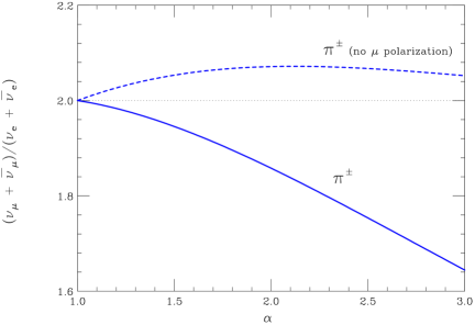
Figure 3: Neutrino flavor ratio $(\nu_{\mu}+\overline{\nu}_{\mu})/(\nu_{e}+\overline{\nu}_{e})$ at the source obtained from the chain decay of charged pions with a power law energy spectrum $\propto E_{\pi}^{-\alpha}$. Energy losses are assumed to be negligible. The dashed line neglects the effect of muon polarization in pion decay.

for a power law spectrum of parent pions is a function of its slope. The ratio is shown in fig. 3. For $\alpha=1$ one has $R_{\mu e}=2$, since in this case the $Z$ factors correspond to the neutrino multiplicities. With increasing $\alpha$ the flavor ratio decreases monotonically, this reflects the fact that the muon neutrinos produced in the direct pion decay are softer than the neutrinos of the muon decay. For the value $\alpha=2$ one has $R_{\mu e}\simeq 1.858$. Figure 3 also shows the predictions obtained neglecting the effects of muon polarization to illustrate the importance of their inclusion.

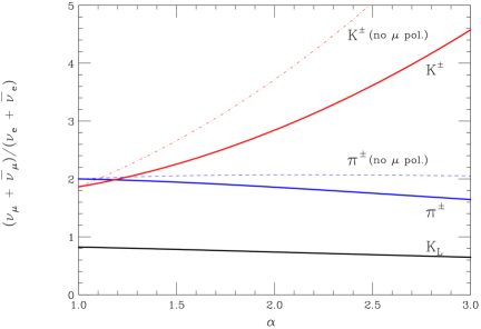
Figure 4: Neutrino flavor ratio $(\nu_{\mu}+\overline{\nu}_{\mu})/(\nu_{e}+\overline{\nu}_{e})$ at the source for the chain decay of different mesons having a power law spectrum $\propto E^{-\alpha}$. The different lines refer to the decay of $\pi^{\pm}$, $K^{\pm}$ and $K_{L}$. The dashed (dotdashed) line show the effect of neglecting muon polarization in the chain decay of charged pions (kaons).

The second most important source of neutrinos is the decay of kaons. Charged kaons can produce neutrinos with three different decay channels: the two body mode $K^{+}\to\mu^{+}\nu_{\mu}$ (with branching ratio 0.6343), and the three body modes $K^{\pm}_{e3}$ ($K^{+}\to\pi^{\circ}e^{+}\nu_{e}$) and $K^{\pm}_{\mu 3}$ ($K^{+}\to\pi^{\circ}\mu^{+}\nu_{\mu}$) that have branching ratios $B^{\pm}_{e3}\simeq 0.0487$ and $B^{\pm}_{\mu 3}\simeq 0.0327$ PDG . The $K_{L}$ can also produce neutrinos in the $K^{\circ}_{e3}$ decay mode ($K_{L}\to\pi^{\mp}e^{\pm}\nu_{e}(\overline{\nu}_{e})$) with combined branching ratio $B^{0}_{e3}\simeq 0.3881$, and $K^{\circ}_{\mu 3}$ mode ($K_{L}\to\pi^{\mp}\mu^{\pm}\nu_{\mu}(\overline{\nu}_{\mu})$) with combined branching ratio $B^{0}_{\mu 3}\simeq 0.2719$. The $R_{\mu e}$ ratios for neutrinos produced by the chain decay of charged or neutral kaons is shown in fig. 4. In the case of charged kaons the 2–body decay mode is the dominant one, the $Z$–factors for this mode have the same form as in pion decay, with the replacement $r_{\pi}\to r_{K}$, however for charged kaons the flavor ratio grows when $\alpha$ increases, reflecting the fact that the muon neutrinos produced in the direct decay carry nearly half ($(1-r_{K})/2\simeq 0.48$) of the parent particle energy while the neutrinos produced in the second stage (from muon decay) take on average only 18% ($\nu_{\mu}$) and 16% ($\nu_{e}$) of the kaon energy. The inclusion of the three body decay modes ($K^{\pm}_{e3}$ and $K^{\pm}_{\mu 3}$) that have smaller branching fractions reduces the flavor ratio, but it is a small correction.

In the case of the decay of $K_{L}$, the three body decays are the only source of neutrinos. The $K^{\circ}_{e3}$ mode has a larger branching fraction than the $K^{\circ}_{\mu 3}$ channel, because of the larger phase space available. When $\alpha=1$, when the flavor ratio reflects the neutrino multiplicities in the final state, the flavor ratio is $R_{\mu e}=2B^{\circ}_{\mu 3}/(B^{\circ}_{e3}+B^{\circ}_{\mu 3})\simeq 0.82$. Increasing $\alpha$ the ratio decreases, because the $\nu_{e}$ from the $K^{\circ}_{e3}$ decay have the hardest spectrum, and their contribution is enhanced.

Note that for power laws with slope $\simeq 2$ the net effect of including kaon decay as a $\nu$ source is a only a small (positive) correction, because of a cancellation between the contributions of charged kaons (that increase the relative importance of muon neutrinos) and neutral kaons (that do the opposite).

VI Energy Loss Mechanisms

In the most general case, the unstable particles that create neutrinos can lose a significant amount of energy during the time that elapses from the moment of their creation to the moment of their decay. This effect can have very important consequences for the spectrum and flavor composition of the neutrinos.

As an illustration, muon energy losses are very important for the prediction of the atmospheric neutrino fluxes. The largest effect is due to the fact that the muons that reach the ground lose rapidly energy because of ionization and electromagnetic radiation processes, and decay practically at rest (or are captured by heavy nuclei Conversi:1947ig ) producing only very low energy neutrinos. Pion energy losses are also very important for the calculation of the atmospheric $\nu$ fluxes. In this case the dominant mechanism for energy loss are hadronic interactions in air. The pion decay length grows linearly with $E_{\pi}$, and (for $E_{\pi}\gtrsim 100$ GeV) it becomes (for vertical particles) comparable to the interaction length. Most pions of higher energy interact before decaying. These hadronic interactions result in a multiplication of the pions, but the secondary particles have much lower energy and the net effect is a strong suppression of the neutrino flux at high energy.

There are several mechanisms for energy loss that could be present in the astrophysical environment where neutrinos are produced. In several circumstances synchrotron radiation could be the dominant source of energy loss Rachen:1998fd ; Kashti . In the presence of a magnetic field of value $B$, the energy loss of a particle of electric charge $e$, mass $m$ and energy $E$, after averaging over all possible orientation of the magnetic field direction is given by the well known expression:

$$-\frac{dE}{dt}=\frac{4}{9}\frac{e^{4}\,B^{2}}{m^{4}}\;E^{2}$$ (32)

The energy loss is significant only for $E\gtrsim E_{\rm syn}$ the critical energy where the the synchrotron loss time $t_{\rm syn}=-[(dE/dt)/E]^{-1}$ is equal to the decay time $t_{\rm dec}=\tau\,E/m$:

$$E_{\rm syn}=\frac{3}{2}\frac{m^{5/2}}{e^{2}\,B\,\sqrt{\tau}}=\frac{5.8\times 10^{18}~{}{\rm eV}}{B_{\rm Gauss}}~{}\left(\frac{m}{m_{\mu}}\right)^{\frac{5}{2}}~{}\left(\frac{\tau}{\tau_{\mu}}\right)^{-\frac{1}{2}}$$ (33)

The critical energy for synchrotron losses scales $\propto m^{5/2}\;\tau^{-1/2}$. It is smallest for muons, it becomes 18.4 times larger for charged pions, and 628 times larger for charged kaons. There is therefore an energy range where the losses are only significant for muons, and a second energy range where the synchroton losses are significant for both pions and muons but not for kaons.

In the presence of ordinary matter in gas form the particles can also lose energy because of ionization and radiation processes (with radiation dominating at large energies). These energy losses take the form $-dE/dt\simeq\rho\,(a+b\,E)$ where $\rho$ is the medium density and $a$ and $b$ are slowly varying coefficients that depend on the gas composition. For a medium mostly composed of protons, as it is likely in astrophysical environments, the critical energy for the energy losses with ordinary matter in gaseous form (where the loss time equals the decay time) is for muons:

$$E^{\mu}_{\rm matter}\simeq 6.5\times 10^{18}~{}(\rho_{-10})^{-1}~{}{\rm eV}$$ (34)

where $\rho_{-10}$ is the matter density in units of $10^{-10}$ g cm^-3.

In the presence of a gas of ordinary matter the dominant source of energy loss for charged pions and kaons is due to hadronic interactions. The critical energy at which the hadronic interaction time $t_{\rm int}=\langle A\rangle/(N_{A}\,\rho\,\sigma_{int})$ equals the decay time $\tau\,E/m$ can be estimated for pions as:

$$E_{\rm matter}^{\pi}\simeq 7.4\times 10^{16}~{}({\rho_{-10})^{-1}~{}{\rm eV}}~{}.$$ (35)

This critical energy scales $\propto m/\tau$ and for charged kaons (assuming the same hadronic cross section) is approximately 7.4 times larger.

The effects of ordinary matter on the secondary particles can be safely neglected for all energies (including those above $E_{\rm matter}$) and all particle types if the density is below the critical value:

$$\rho_{\rm crit}\simeq 2.0\times 10^{-15}~{}B_{\rm Gauss}~{}{\rm g~{}cm}^{-3}~{}.$$ (36)

For $\rho<\rho_{\rm crit}$ the energy losses on matter are either negligibly small, or dominated by the synchrotron losses.

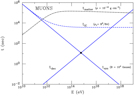
Figure 5: Characteristic times for a muon plotted as a function of its energy. The different lines correspond to (i) the decay time $t_{\rm dec}$; (ii) the time $t_{\rm matter}$ for energy loss in ordinary matter, assuming a gaseous medium with the average composition of the interstellar medium (ISM) and the density $\rho=10^{-10}$ g cm^-3 (this time scales as $t_{\rm matter}\propto\rho^{-1}$); (iii) the time $t_{\rm syn}$ for synchrotron losses in a magnetic field $B=10^{4}$ Gauss ($t_{\rm syn}\propto B^{-1}$), and (iv) the time $t_{IC}$ for Inverse Compton losses. The target radiation field is assumed isotropic, with energy spectrum of GRB form (63) with $\varepsilon_{\rm b}=1$ KeV, and energy density $\rho_{\gamma}=\rho_{B}$ (with $B=10^{4}$ Gauss).

Figures 5 and 6 illustrate the above discussion showing the characteristic times $t_{\rm dec}$ (decay), $t_{\rm syn}$ (synchrotron losses) and $t_{\rm matter}$ for muons and pions.

Gamma Ray Bursts have been proposed by Waxman and Bahcall Waxman-grb as a neutrino source having a potentially very strong magnetic field. In the WB model, the strength of the magnetic field is estimated by energy equipartition, assuming that it corresponds to an energy density of the same order of magnitude as the energy density carried by the fireball photons. It is natural to ask the question if this radiation field can be an important source of energy loss for secondary particles produced in it. The calculation of the time $t_{IC}$ for Inverse Compton losses of charged particles traveling in the fireball radiation field requires to take into account the energy spectrum of the target photons (assumed to be isotropic in the GRB jet frame). In fact the Compton scatterings with sufficiently high energy photons $\varepsilon\gtrsim m^{2}/E$ happen in the Klein–Nishina regime and are inefficient as a source of energy loss. For the predicted GRB photon spectrum Waxman-grb , (given also in equation (63)) that falls at high energy $\propto\varepsilon^{-2}$, the energy loss for Inverse Compton grows at high energy as $-(dE/dt)_{IC}\propto E\,\rho_{\gamma}/m^{2}$, (where $\rho_{\gamma}$ is the target photon energy density), and the loss time $t_{IC}$ becomes constant. The results of a detailed integration are also shown in fig. 5 and 6, where we have assumed that the densities $\rho_{B}=B^{2}/(8\pi)$ and $\rho_{\gamma}$ are equal. In most circumstances (unless equipartition is very badly violated) Inverse Compton losses can be neglected.

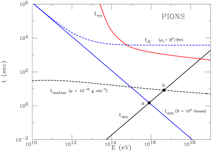
Figure 6: Characteristic times for charged pions. The different lines correspond to: (i) the decay time $t_{\rm dec}$; (ii) the time $t_{\rm matter}$ for hadronic interactions with a gaseous medium with the ISM composition and density $\rho=10^{-10}$ g cm^-2; (iii) the time $t_{\rm syn}$ for synchrotron losses (in a randomly oriented magnetic field $B=10^{4}$ Gauss); (iv) the time $t_{IC}$ for Inverse Compton losses; (v) the time $t_{\pi\gamma}$ for photo–hadronic interactions. The last two times are calculated for a radiation field of GRB form (63) with $\varepsilon_{\rm b}=1$ KeV, and energy density $\rho_{\gamma}=\rho_{B}$ (with $B=10^{4}$ Gauss). Point a (b) is the intersection of the $t_{\rm dec}$ and $t_{\rm syn}$ ($t_{\rm matter}$) curves. The energy that correspond to the point is the critical energy above which synchrotron losses (the hadronic interaction probability) are (is) important before decay. For the values of $B$ and $\rho$ chosen in this illustration the presence of a gas of ordinary matter is negligible.

Charged pions (and kaons) traveling in a radiation field can also lose energy for photo–hadronic interactions. For completeness we have calculated the interaction time of pions in the GRB radiation field. The result is also shown in fig. 6. For this calculation the $\pi\gamma$ hadronic cross section has been estimated as the sum of contributions for production of the relevant resonances PDG : $\rho(770)$, $a1(1260)$, $b1(1235)$ and $a2(1320)$ and a non resonant background. At high energy ($s\gtrsim 30$ GeV²) the cross section is described by a formula obtained using Pomeron universality and Regge poles factorization from the fits to the $\gamma$-proton and $\pi$-proton cross sections reported in PDG . The lower energy non–resonant background has been normalized to obtain a smooth energy dependence.

At very high energy pion–photon interactions are more important that Inverse Compton losses, however if the energy density in photons and magnetic field are comparable, the synchrotron losses dominate.

VI.1 Decay Energy Distribution

To describe the effect of energy losses, it is useful to consider the function $dp_{\rm dec}/dE(E,E_{i})$ that gives the probability density for an unstable particle of mass $m$ and lifetime $\tau$, created with initial energy $E_{i}$ to decay with energy $E$. Assuming that the energy loss is a continuous process, and can be described by the equation:

$$-\frac{dE}{dt}(E)=f(E)~{},$$ (37)

(with $f(E)$ is the average loss per unit time), the distribution $dp_{\rm dec}/dE(E,E_{i})$ can be calculated as:

$$\frac{dp_{\rm dec}}{dE}(E;E_{i})=\frac{m}{\tau}\;\frac{1}{f(E)\;E}~{}\exp\left[-\frac{m}{\tau}\;\int_{E}^{E_{i}}\frac{dE^{\prime}}{f(E^{\prime})\,E^{\prime}}\right].$$ (38)

For an energy loss of form $f(E)=a\,E^{n}$ (with $n>0$) the decay probability becomes Kashti :

$$\frac{dp_{\rm dec}}{dE}(E;E_{i})=\frac{\epsilon^{n}}{E^{n+1}}~{}\exp\left[-\frac{\epsilon^{n}}{n}\;\left(\frac{1}{E^{n}}-\frac{1}{E_{i}^{n}}\right)\right]$$ (39)

with:

$$\epsilon=\left(\frac{m}{\tau\,a}\right)^{\frac{1}{n}}.$$ (40)

The quantity $\epsilon$ has the physical meaning of the energy for which the loss-time: $t_{\rm loss}=E/f(E)=1/(a\,E^{n-1})$ is equal to the decay time: $t_{\rm decay}=\tau\,E/m$.

For $E_{i}\ll\epsilon$, the energy loss is negligible and the decay energy distribution becomes a simple delta function:

$$\left(\frac{dp_{\rm dec}}{dE}(E;E_{i})\right)_{E_{i}\ll\epsilon}\simeq\delta[E-E_{i}],$$ (41)

while for $E_{i}\gg\epsilon$ the decay energy distribution takes a universal form

$$\left(\frac{dp_{\rm dec}}{dE}(E;E_{i})\right)_{E_{i}\gg\epsilon}=\frac{\epsilon^{n}}{E^{n+1}}~{}\exp\left[-\frac{1}{n}\frac{\epsilon^{n}}{E^{n}}\right].$$ (42)

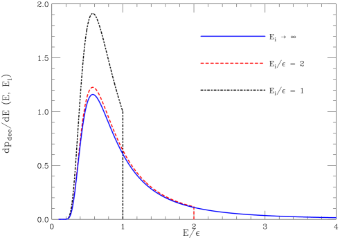
Figure 7: Decay energy distribution $dp_{\rm dec}/dE(E,E_{i})$ for particles losing energy as $-dE/dt=a\,E^{2}$. The critical energy $\epsilon=\sqrt{m/(a\tau)}$ is the energy where the decay time and the energy loss time are equal.

An illustration of the decay energy distribution for the case $f(E)=a\;E^{2}$, relevant for synchrotron emission is shown in fig. 7. The important qualitative feature in fig. 7 is that all particles with sufficiently high initial energy ($E_{i}\gtrsim 2~{}\epsilon$) have nearly identical final energy distributions, with a well defined maximum at $E\sim 0.6\,\epsilon$. In many cases this can result in “pile–up” effects in the final state particle spectra.

VII Hadronic interactions

The target for the primary particles interactions can be either normal matter in gaseous form, or a radiation field. In the following we will consider both cases separately.

VII.1 Gas Target

For a target material made of normal matter at rest the interaction rate of a primary particle of energy $E_{p}$ is:

$$K_{pp}(E_{p})=n_{\rm gas}~{}\sigma_{pp}(s).$$ (43)

where $n_{\rm gas}$ is the number density of the target material. Equation (43) is valid for a situation where the primary particles are protons and the target material is also dominated by protons. This is likely to be a good approximation in most circumstances. It is straightforward to consider the more general case.

Since the target is at rest, the interaction rate is proportional to the cross section at a well defined c.m. energy $s=m_{p}^{2}+2m_{p}\,E_{p}$. Since hadronic cross sections grow only logarithmically with c.m. energy (or as power law $\propto s^{\epsilon}$ with a small exponent $\epsilon$), the interaction rate of the primary particles changes only very slowly with energy.

It is well known that the multiplicity and energy distributions of the particles produced in hadronic interactions cannot be calculated from first principles, however it is believed that particle production, to a a reasonably good approximation, satisfies Feynman scaling, defined by the condition:

$$E\;{d\sigma_{j}\over dp_{\parallel}^{*}}(p_{\parallel}^{*},\sqrt{s})=F_{j}(x_{F})$$ (44)

where $p_{\parallel}^{*}$ is the longitudinal momentum in the c.m. frame, $d\sigma_{j}$ is the inclusive differential cross section for the production of particle type $j$, and $x_{F}=2\,p_{\parallel}^{*}/\sqrt{s}$ is the Feynman variable.

For large c.m. energy ($s\gg m_{p}^{2}$) the target rest frame energy of secondary particles in the forward hemisphere ($x_{F}>0$) is well approximated by the expression $E\simeq E_{p}\;x_{F}$ (where $E$ ($E_{p}$) is the energy of the final state (projectile) particle in this frame). It follows that the validity of Feynman–scaling in the fragmentation region implies also the approximate validity of scaling of the inclusive cross sections in the target rest frame:

$${dn_{pp\to a}\over dE}(E;E_{p})\simeq{1\over E_{p}}~{}F_{pp\to a}\left({E\over E_{p}}\right)~{}~{}~{}~{}~{}~{}({\rm for}~{}~{}E\gg m)$$ (45)

The approximate validity of the scaling law (45) together with the slow variation of the hadronic cross sections with c.m. energy have the important consequence (based on essentially the same argument previously discussed in connection with decay (25)) that a power law spectrum of primary particles generates spectra of secondaries also having a power law form. For example for final state particles of type $\pi$:

$$Q_{\pi}(E_{\pi}) = C_{p}\;n_{\rm gas}\;\sigma_{pp}\;E_{\pi}^{-\alpha}~{}\int_{0}^{1}~{}dx~{}x^{\alpha-1}~{}F_{pp\to\pi}(x)=C_{p}\;n_{\rm gas}\;\sigma_{pp}\;Z_{pp\to\pi}(\alpha)\;E_{\pi}^{-\alpha}~{}.$$ (46)

In general, one expects some deviations from a perfect power law. First of all, this can reflect a shape of the primary spectrum different from a power law. In addition the energy dependence of the cross sections, and the existence of violations of Feynman scaling (as measured in hadron colliders) introduce some distortions. Another situation that can result in large deviations from a power law emission arises when particles of different rigidities have different confinement volumes having different target densities (while our derivation of (46) implicitely assumed a homogeneous source volume).

VII.2 Photoproduction

In several of the proposed neutrino sources, the target of the primary particles is a radiation field. In this case the interaction rate and the energy distribution of the particles produced in an interaction depend not only on the density, but also on the energy and angular distribution of the target photons. The interaction probability per unit time of a proton of energy $E_{p}$ traveling in the radiation field described by $n_{\gamma}(\varepsilon,\Omega_{\gamma})$ can be calculated as:

$$K_{p\gamma}\left(E_{p}\right)=\frac{1}{\lambda_{p\gamma}(E_{p})}=\int d\varepsilon~{}\int_{-1}^{+1}\;\frac{d\cos\theta_{p\gamma}}{2}\;(1-\cos\theta_{p\gamma})~{}n_{\gamma}(\varepsilon,\cos\theta_{p\gamma})~{}\sigma_{p\gamma}(\epsilon_{r})$$ (47)

where $\theta_{p\gamma}$ is the angle between the photon and the proton momenta in the interaction, $\sigma_{p\gamma}$ is the photoproduction cross section, and $\epsilon_{r}$ is the photon energy in the proton rest frame:

$$\epsilon_{r}=\frac{E_{p}\,\varepsilon}{m_{p}}\;(1-\cos\theta_{p\gamma})$$ (48)

The quantity $\epsilon_{r}$ is in one to one correspondence with the c.m. energy of the reaction. It is convenient to change the integration variable from $\cos\theta_{p\gamma}$ to $\epsilon_{r}$. Restricting ourselves to a situation (and a frame) where the photon distribution is isotropic one can then rewrite (47) as:

$$K_{p\gamma}(E_{p})=\frac{1}{2}\,\frac{m_{p}^{2}}{E_{p}^{2}}\;~{}\int_{\epsilon_{\rm th}}^{\infty}\;d\epsilon_{r}~{}\epsilon_{r}~{}\sigma_{p\gamma}(\epsilon_{r})\int_{(m_{p}\epsilon_{r})/(2E_{p})}^{\infty}\;d\varepsilon~{}\frac{n_{\gamma}(\varepsilon)}{\varepsilon^{2}}$$ (49)

where $\epsilon_{\rm th}$ is the threshold photon energy for pion production in the proton rest frame:

$$\epsilon_{\rm th}=m_{\pi}+\frac{m_{\pi}^{2}}{2m_{p}}$$ (50)

Equation (49) can be recast in the form

$$K_{p\gamma}(E_{p})=~{}\int_{\epsilon_{\rm th}}^{\infty}\;d\epsilon_{r}~{}f_{p\gamma}\left(\epsilon_{r};~{}E_{p}\right)~{}.$$ (51)

This expression shows explicitely the fact that the $p\gamma$ interactions of a proton of energy $E_{p}$ do not correspond to a single value of the c.m. energy but have a distribution, that in general is a function of $E_{p}$, and is determined by the energy (and angular) distribution of the target photons. The probability distribution for $\epsilon_{r}$ is:

$$p(\epsilon_{r};~{}E_{p})=\frac{f(\epsilon_{r},E_{p})}{K_{p\gamma}(E_{p})}~{}.$$ (52)

A phenomenologically important case for the target radiation field is the form: $n_{\gamma}(\varepsilon)=C_{\gamma}\,\varepsilon^{-\beta}$, that is an (isotropic) power law spectrum of slope $\beta$. For this form the last integration in (49) can be performed analytically with the result:

$$K_{p\gamma}(E_{p})=C_{\gamma}\;\frac{2^{\beta}}{\beta+1}\;\left(\frac{E_{p}}{m_{p}}\right)^{\beta-1}~{}\int_{\epsilon_{\rm th}}^{\infty}~{}d\epsilon_{r}~{}\epsilon_{r}^{-\beta}~{}\sigma_{p\gamma}(\epsilon_{r})=K_{0}(\beta)~{}E_{p}^{\beta-1}$$ (53)

One can see that the interaction rate has the energy dependence $E_{p}^{\beta-1}$. The growth with energy (for $\beta>1$) of the interaction rate can be understood observing that a proton of energy $E_{p}$ can interact inelastically only with photons above a minimum energy $m_{p}\,\epsilon_{\rm th}/(2E_{p})$. This minimum target energy decreases proportionally to $E_{p}^{-1}$, and therefore protons of higher energy can interact with a softer and more abundant photon population. A result essentially equivalent to equation (53) was originally shown by Waxman and Bahcall in Waxman-grb . An important feature of equation (53) is that the probability distribution for $\epsilon_{r}$ takes a form that is independent from $E_{p}$:

$$p(\epsilon_{r})=\epsilon_{r}^{-\beta}~{}\sigma_{p\gamma}(\epsilon_{r})\left[\int_{\epsilon_{\rm th}}^{\infty}~{}d\epsilon_{r}~{}\epsilon_{r}^{-\beta}~{}\sigma_{p\gamma}(\epsilon_{r})\right]^{-1}$$ (54)

This fact has interesting consequences discussed below. It should be noted however that equations (53) and (54) are calculated assuming a power law that extends to very large energy without any cutoff. This is not only unrealistic, but in some important cases also untenable. In fact the integral over $\epsilon_{r}$ in (53) diverges at its upper limit (since $\sigma_{p\gamma}$ is slowly increasing with energy) for $\beta\leq 1$, and the expression for $K_{p\gamma}$ becomes meaningless. The divergence corresponds to the divergence of the photon number density in the absence of an upper limit cutoff (note that in fact the energy density of the photon population diverges at the upper end already for $\beta\leq 2$). The introduction of a high energy cutoff for the energy distribution of the target photons is therefore mandatory. This will be discussed in the next section.

The properties of particle production in $p\gamma$ interactions is clearly intimately related to the distribution of c.m. energy (or equivalently $\epsilon_{r}$) of the interactions. It is necessary to consider the energy distributions of secondary particles in the “source frame” (where the primary proton has energy $E_{p}$). In this frame the energy of a secondary particle can obviously be expressed as function of quantities in the c.m. frame with an appropriate Lorentz boost:

$$E=\gamma\;(E^{*}+v\,p_{z}^{*})$$ (55)

where $v$ and $\gamma$ are the velocity and gamma–factor of the c.m. of the reaction in the source frame, $E^{*}$ is the c.m. energy of the secondary particle and $p_{z}^{*}$ the momentum component parallel to $\beta$. The Lorentz $\gamma$ that connects the source and c.m. frames is:

$$\gamma=\frac{E_{p}+\varepsilon}{\sqrt{s}}\simeq\frac{E_{p}}{\sqrt{s}}~{}.$$ (56)

In the second approximated equality we have neglected the photon energy $\varepsilon$ with respect to $E_{p}$, this is expected to be an excellent approximation. Similarly one can safely make the approximation $v\simeq 1$. With these approximations we can rewrite the Lorentz boost from the c.m. to the source frame as:

$$E=E_{p}\;\frac{E^{*}+p_{z}^{*}}{\sqrt{s}}=E_{p}\;\xi~{}.$$ (57)

This equations indicates that to a good approximation all secondary particles of source frame energy $E$ are created in the c.m. frame of the interaction with (to a very good approximation) the same value of the quantity $\xi=(E^{*}+p_{z}^{*})/\sqrt{s}$. The energy spectrum of (for example) pions created in the interaction of a proton of energy $E_{p}$ can then be written as:

$$\frac{dn_{p\gamma\to\pi}}{dE_{\pi}}(E_{\pi};~{}E_{p})\simeq\frac{1}{E_{p}}~{}\int_{\epsilon_{\rm th}}^{\infty}d\epsilon_{r}~{}p(\epsilon_{r};E_{p})~{}\left[\frac{dn_{p\gamma\to\pi}}{d\xi}(\xi;~{}\epsilon_{r})\right]_{\xi=E_{\pi}/E_{p}}$$ (58)

where $dn_{p\gamma\to\pi}/d\xi(\xi,\epsilon_{r})$ is the $\xi$ distributions of the secondary particles of type $\pi$ in $p\gamma$ interactions with c.m. energy that correspond to $\epsilon_{r}$; this distribution is convoluted for a fixed value $\xi=E_{\pi}/E_{p}$ over all possible value of the $\epsilon_{r}$ with the appropriate distribution. If the energy distribution of the target photon field has a power law form, the function $p(\epsilon_{r};~{}E_{p})$ is independent from $E_{p}$, and equation (58) becomes the expression of a scaling law of form:

$$\frac{dn_{p\gamma\to\pi}}{dE_{\pi}}(E_{\pi};~{}E_{p})\simeq\frac{1}{E_{p}}~{}F_{p\gamma\to\pi}\left(\frac{E_{\pi}}{E_{p}};~{}\beta\right)~{}.$$ (59)

The scaling function $F_{p\gamma\to\pi}$ is not truly universal, but depends on the slope of the target photon spectrum. Integrating over all primary particle energies one can obtain the production rate of pions as:

$$Q_{\pi}(E_{\pi}) = \int_{E_{\pi}}^{\infty}~{}dE_{p}~{}N_{p}(E_{p})~{}K_{p\gamma}(E_{p})~{}{dn_{p\gamma\to\pi}\over dE_{\pi}}(E_{\pi};E_{p})$$ (60)

$$= \int_{E_{\pi}}^{\infty}~{}dE_{p}~{}\left(C_{p}\;E_{p}^{-\alpha}\right)~{}~{}\left(K_{0}(\beta)\;E_{p}^{\beta-1}\right){1\over E_{p}}~{}F_{p\gamma\to\pi}\left(\frac{E_{\pi}}{E_{p}};~{}\beta\right)$$

$$= C_{p}\;K_{0}(\beta)E_{\pi}^{-(\alpha-\beta+1)}~{}\int_{0}^{1}~{}d\xi~{}\xi^{\alpha-\beta}~{}F_{p\gamma\to\pi}(\xi;~{}\beta)$$

$$= C_{p}\;K_{0}(\beta)\;Z_{p\gamma\to\pi}[\alpha-\beta+1,\beta]\;E_{\pi}^{-(\alpha-\beta+1)}~{}~{}.$$

This equation shows that under the assumptions made, that is: (i) a power law spectrum of protons, and (ii) an isotropic power law spectrum of target photons, the energy distribution of produced secondaries is again a power law with slope $\alpha-\beta+1$. Note that this result is based on purely kinematical considerations, while the result (46) about the interactions on an ordinary matter target was based on a dynamical assumption about the approximate validity of Feynman scaling in hadronic interactions, and on the weak energy dependence of hadronic cross sections.

A result roughly equivalent to (60) was obtained by Waxman and Bahcall in Waxman-grb , who concluded that in the case $\beta=1$ the neutrino emission has a power law spectrum with the same slope of the parent protons. However, the validity of equation (60), as the validity of equation (53), relies on the untenable assumption that the power law spectrum of target photons has no high energy cutoff. The important effects of the existence of an high energy cutoff for equations (53) and (60) will be discussed in section VIII.

VII.3 Nuclear photodisintegration

The beta decay of neutrons produces $\overline{\nu}_{e}$. In many circumstances the contribution of this anti–neutrino source is of negligible importance. This is because the average fraction of the neutron energy $E_{n}$ carried away by the $\overline{\nu}_{e}$ (in a frame where the neutron is ultrarelativistic) is $\langle E_{\overline{\nu}_{e}}\rangle/E_{n}\simeq 5.1\times 10^{-4}$, with end–point $E^{\rm max}_{\overline{\nu}_{e}}/E_{n}\simeq 2(m_{n}-m_{p}-m_{e})/m_{n}\simeq 1.66\times 10^{-3}$. In most cases the flux of the softer $n$–decay neutrinos is neglible with respect to the contribution of neutrinos from $\pi/K$ of decay that carry a much larger fraction (of order $\sim 0.25$) of their parent energy. There are two circumstances where the $n$ contribution can become important. The first one is when the neutrino spectrum has a low energy cutoff. This happens naturally when the target of the primary particles is a radiation field and there is an interaction energy threshold. In this case the $\overline{\nu}_{e}$ produced in neutron decay can become the dominant component of the neutrino flux at low energy, because most of the neutrinos from pion and kaon decay have higher energy. An example of this situation will be shown in the following section. A second, more interesting case is when the neutrons are produced in the photodisintegration of high energy nuclei neutron-decay . In this case it is in principle possible to have the emission of a pure $\overline{\nu}_{e}$ flux. In fact the threshold for photodisintegration of a nucleus of mass number $A$ expressed in terms of energy per nucleon ($E_{0}=E_{\rm tot}/A$) is of order:

$$\left(E_{0}\right)_{\rm th}^{\gamma A}\simeq\frac{m_{p}\epsilon_{\rm bind}}{2\;\varepsilon_{\gamma}}$$ (61)

where $\varepsilon_{\gamma}$ is the energy of the target photons and $\epsilon_{\rm bind}\simeq 8$ MeV is the binding energy of a nucleon in the nucleus. The threshold for pion photoproduction is:

$$\left(E_{0}\right)_{\rm th}^{\pi}\simeq\frac{m_{p}\;m_{\pi}}{2\;\varepsilon_{\gamma}}\left(1+\frac{m_{\pi}^{2}}{2\,m_{p}}\right)~{}.$$ (62)

Since the binding energy $\epsilon_{\rm bind}$ is approximately fifteen times smaller than a pion mass, it is in principle possible to have circumstances where the primary particles are below the threshold for pion production, but above the threshold for photodisintegration. This would clearly result in a pure $\overline{\nu}_{e}$ flux. It should be noted that the photodisintegration and pion photoproduction thresholds differ by only one order of magnitude, and therefore a pure $\overline{\nu}_{e}$ flux can only extend for a small interval of energy. In general one expects important contributions from neutrinos from meson decays. In fact, even a very small number of pion production interactions created by the high energy tails of the photon and/or primary particles spectra can result in an important “contamination” of $\nu_{e}$ and muon neutrinos. Most of these neutrinos have an energy two orders of magnitude larger that the $\overline{\nu}_{e}$ produced in $n$ decay and have a correspondingly larger cross section.

VIII Neutrino Production in Gamma Ray Bursts

As an illustration of the spectra and flavor composition of neutrinos from astrophysical sources, in this section we will consider the model of neutrino production in Gamma Ray Bursts (GRB) developed by Waxman and Bahcall (WB) Waxman-grb . Our goal is not to analyze critically the assumptions that underline the model, but to recalculate with a more detailed modeling of particle production the neutrino fluxes starting from the same general assumptions.

In the (WB) model Waxman-grb the GRB prompt emission is generated by the synchrotron radiation of high energy electrons accelerated by internal shocks in a relativistic expanding wind (for more discussion see Piran-grb ; zhang-meszaros ; alternative explanations of the GRB mechanism exist in the literature, see for example dar-derujula-grb ).

The internal shocks also accelerate protons, that can interact with the radiation field of the wind and produce secondary particles that generate neutrinos. The accelerated protons have a power law spectrum of slope $\alpha\simeq 2$, while the target radiation field is isotropic in the wind frame, and approximated as a broken power law of form:

$$n_{\gamma}(\varepsilon)=\cases{C_{\gamma}\;\varepsilon^{-1}&for $\varepsilon\leq\varepsilon_{\rm b}$,\cr C_{\gamma}\;\varepsilon_{\rm b}\;\varepsilon^{-2}&for $\varepsilon>\varepsilon_{\rm b}$}$$ (63)

where $\varepsilon_{\rm b}$ is a break energy. The photon energy distribution in the wind frame is related to the obervable spectrum of the GRB prompt emission by a Lorentz transformation with parameter $\Gamma\simeq 300$. Since the observed break energies are distributed around an average value $\langle\varepsilon_{\rm b}^{\rm obs}\rangle\sim 300$ KeV batse , the typical value of $\varepsilon_{\rm b}$ in the wind frame is of order 1 KeV.

The energy spectra of individual GRB are indeed well fitted by two power laws smoothly joined at a break energy, however the fitted values of the exponents of the spectrum have rather broad distributions centered at $\beta\simeq 1$ below the break energy, and $\beta\simeq 2.2$ above the break energy batse . In our calculation we have therefore considered a generalization of (63) that leaves the two exponents as free parameters. We have also introduced a high energy cutoff $\varepsilon_{\rm max}$, because in its absence the energy density of the radiation field would diverge for a high energy slope $\leq 2$. Our description of the energy spectrum of the target radiation field then becomes:

$$n_{\gamma}(\varepsilon)=\cases{(C_{\gamma}/\varepsilon_{\rm b})\;(\varepsilon/\varepsilon_{\rm b})^{-\beta_{1}}&for $\varepsilon\leq\varepsilon_{\rm b}$,\cr(C_{\gamma}/\varepsilon_{\rm b})\;(\varepsilon/\varepsilon_{\rm b})^{-\beta_{2}}&for $\varepsilon_{\rm b}<\varepsilon<\varepsilon_{\rm max}$,\cr 0&for $\varepsilon\geq\varepsilon_{\rm max}$.\cr}$$ (64)

The calculation of the interaction rate of a proton of energy $E_{p}$ in such a radiation field is straightforward. The target photon field (64) can be seen as the sum of two power law spectra with sharp low and high–energy cutoffs $\varepsilon_{\rm min}$ and $\varepsilon_{\rm max}$.

We have already obtained the expression for the proton interaction rate for a power law that extends to all energies. The expression (53) must however be modified in the presence of low and high energy cutoffs. In the presence of a high energy cutoff $\varepsilon_{\rm max}$ the interaction rate vanishes below a threshold energy $E_{\rm th}$. Above the threshold, in the interval:

$$E_{\rm th}=\frac{m_{p}\;\epsilon_{\rm th}}{2\,\varepsilon_{\rm max}}\leq E_{p}\leq\frac{m_{p}\;\epsilon_{\rm th}}{2\,\varepsilon_{\rm min}}.$$ (65)

the interaction rate is

$$K_{p\gamma}(E_{p})=\frac{2^{\beta}\,C_{\gamma}}{\beta+1}\;\left(\frac{E_{p}}{m_{p}}\right)^{\beta-1}~{}\int_{\epsilon_{\rm th}}^{2E_{p}\varepsilon_{\rm max}/m_{p}}~{}d\epsilon_{r}~{}\sigma_{p\gamma}(\epsilon_{r})~{}\left[\epsilon_{r}^{-\beta}-\epsilon_{r}\,\left(\frac{m_{p}}{2E_{p}\,\varepsilon_{\rm max}}\right)^{\beta+1}\right]$$ (66)

coinciding with (53) in the limit $\varepsilon_{\rm max}\to\infty$. The effect of a lower energy cutoff $\varepsilon_{\rm min}$ is to stop the $E_{p}^{\beta-1}$ growth of the interaction rate. For $E_{p}>m_{p}\epsilon_{\rm th}/(2\varepsilon_{\rm min})$ equation (66) must be replaced by:

$$K_{p\gamma}(E_{p}) = \frac{C_{\gamma}\,m_{p}^{2}}{2\,E_{p}^{2}\,(1+\beta)}~{}(\varepsilon_{\rm min}^{-(\beta+1)}-\varepsilon_{\rm max}^{-(\beta+1)})~{}~{}\int_{\epsilon_{\rm th}}^{2E_{p}\,\varepsilon_{\rm min}/m_{p}}~{}d\epsilon_{r}~{}\epsilon_{r}~{}\sigma_{p\gamma}(\epsilon_{r})$$ (67)

$$+ \frac{2^{\beta}\,C_{\gamma}}{\beta+1}\;\left(\frac{E_{p}}{m_{p}}\right)^{\beta-1}\int_{2E_{p}\varepsilon_{\rm min}/m_{p}}^{2E_{p}\varepsilon_{\rm max}/m_{p}}~{}d\epsilon_{r}~{}\sigma_{p\gamma}(\epsilon_{r})~{}\left[\epsilon_{r}^{-\beta}-\epsilon_{r}\,\left(\frac{m_{p}}{2E_{p}\,\varepsilon_{\rm max}}\right)^{\beta+1}\right]~{}~{}~{}~{}$$

For a qualitative understanding, it can be useful to consider the $p\gamma$ cross section as approximately constant above threshold. The integrations over $\epsilon_{r}$ in (66) and (67) are then trivial. For $\beta\neq 1$ one finds:

$$\left[K_{p\gamma}(E_{p})\right]^{\beta\neq 1}\simeq\cases{0&for $x<1$\cr C_{\gamma}\,\sigma_{p\gamma}~{}\left(\frac{2\,\varepsilon_{\rm max}^{1-\beta}}{\beta^{2}-1}\right)~{}\left[x^{\beta-1}-\frac{1}{2}\left(1+\beta+(1-\beta)\,x^{-2}\right)\right]&for $1\leq x\leq r$\cr C_{\gamma}\,\sigma_{p\gamma}~{}\varepsilon_{\rm min}^{1-\beta}~{}\left[\frac{1-r^{1-\beta}}{\beta-1}-\frac{1}{x^{2}\,(1+\beta)}\;\left(r^{2}-r^{1-\beta}\right)\right]&for $x>r$}$$ (68)

where $x=E_{p}/E_{\rm th}$ is the proton energy expressed in units of the threshold energy, and $r=\varepsilon_{\rm max}/\varepsilon_{\rm min}$. For $\beta=1$, one finds:

$$\left[K_{p\gamma}(E_{p})\right]^{\beta=1}\simeq\cases{0&for $x<1$\cr C_{\gamma}\,\sigma_{p\gamma}~{}\left[\log[x]-\frac{1}{2}\,\left(1-\frac{1}{x^{2}}\right)\right]&for $1\leq x\leq r$\cr C_{\gamma}\,\sigma_{p\gamma}~{}\left[\log[r]-\frac{1}{2\,x^{2}}\,\left(r^{2}-1\right)\right]&for $x>r$\cr}$$ (69)

These expressions show that the interaction rate for a power law spectrum of target photons in a restricted range do maintain the approximate behaviour $K_{p\gamma}\propto E_{p}^{\beta-1}$ but only in a limited energy region (in the limit $\beta\to 1$ the interaction rate grows logarithmically: $K_{p\gamma}\propto\log[E_{p}\,\varepsilon_{\rm max}]$). The interaction probability vanishes below threshold and goes asymptotically to a constant for very large $E_{p}$. It can also be useful to consider the high energy limit ($E_{p}/E_{\rm th}\to\infty$) of expressions (68) and (69):

$$\left[K_{p\gamma}(E_{p})\right]^{\beta\neq 1}_{E_{p}\to\infty}=\sigma_{p\gamma}\;\frac{C_{\gamma}}{\beta-1}~{}\left(\varepsilon_{\rm min}^{-\beta+1}-\varepsilon_{\rm max}^{-\beta+1}\right)~{},$$ (70)

$$\left[K_{p\gamma}(E_{p})\right]^{\beta=1}_{E_{p}\to\infty}=\sigma_{p\gamma}\;C_{\gamma}~{}\log\left[\frac{\varepsilon_{\rm max}}{\varepsilon_{\rm min}}\right]~{}.$$ (71)

These expressions have the form $K_{p\gamma}=\sigma_{p\gamma}\;N_{\gamma}$ with $N_{\gamma}$ the integrated number density of the target photons, that can be immediately recognized as the correct high energy limit.

The interaction probability for the radiation field (64) can be obtained combining two expressions corresponding to the parts of the photon spectrum below and above the break energy $\varepsilon_{\rm b}$ that plays in the two cases the role of the maximum or the minimum target photon energy. An illustration of the energy dependence of the proton interaction rate is shown in figure 8. The curves in this and the following figures are made independent from the value of $\varepsilon_{\rm b}$ measuring all energies in units of:

$$E^{*}=\frac{m_{p}\,\epsilon_{\rm th}}{2\,\varepsilon_{\rm b}}=\frac{m_{p}\,m_{\pi}}{2\,\varepsilon_{\rm b}}\;\left(1+\frac{m_{\pi}}{2\,m_{p}}\right)\simeq 6.9\times 10^{13}~{}\left(\frac{\varepsilon_{\rm b}}{\rm KeV}\right)^{-1}~{}{\rm eV}.$$ (72)

The energy $E^{*}$ has the physical meaning of the threshold proton energy for inelastic interactions with photons having the break energy $\varepsilon_{\rm b}$. In figure 8 we have chosen for the target photons energy spectrum the original form (63) with exponents $\beta_{1}=1$, $\beta_{2}=2$ and no high energy cutoff. For low $E_{p}$ the interaction rate grows approximately linearly with energy according to the scaling law (53) because low energy protons interact inelastically only with the high energy part of the radiation field (with slope $\beta_{2}=2$). For larger energy ($E_{p}\gtrsim E^{*}$) the growth becomes logarithmic following the qualitative behaviour of equation (69). It should be noted that the assumption made in Waxman-grb of considering the interaction rate as approximately constant for $E_{p}>E^{*}$ is not a good approximation.

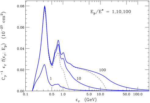
Figure 9: Distribution of $\epsilon_{\rm r}$ (the photon energy in the proton rest frame) for the $p\gamma$ interactions of protons of different energy $E_{p}$. The isotropic photon field has the energy spectrum of GRB form (63). The dashed line neglect the contribution of photons above the break energy $\varepsilon_{\rm b}$.

In fig. 9 we show the distribution $f(\epsilon_{r};~{}E_{p})$ of the c.m. energy of the interaction for different values of the proton energy ($E_{p}/E^{*}=1$, 10, 100). The distribution is proportional to the $p\gamma$ cross section, and the shape of the curves in the figure reflects the energy dependence of $\sigma_{p\gamma}$ that has prominent resonances. The most important one (at $\epsilon_{r}\sim 0.3$ GeV) corresponds to the production of the $\Delta$ resonance. The important feature in the figure is that with increasing energy, higher and higher c.m. energies become possible. This has significant phenomenological consequences. For example, for $\epsilon_{r}$ sufficiently small, only production of a single pion, in the two channels $p\pi^{\circ}$ and $n\pi^{+}$, is kinematically allowed, and therefore there is no $\pi^{-}$ production, and consequently no $\overline{\nu}_{e}$ production. For larger c.m. energy multiple pion production becomes possible, $\overline{\nu}_{e}$ can be produced, and the ratio $\nu_{e}/\overline{\nu}_{e}$ decreases. Above the $K\Lambda$ energy threshold, also the production of kaons becomes possible introducing an additional neutrino source.

In the following we will show some examples of the neutrino fluxes that are obtained varying the parameters of the model. Our calculations have been performed by Montecarlo methods using a detailed model for the $p\gamma$ cross section that includes the production of all relevant resonances and a non–resonant component photo-mc . In order to perform a calculation one needs to specify: (i) the primary proton spectrum, (ii) the target photon spectrum, and finally the value of the magnetic field $B$ (all other sources of energy losses for secondary particles are considered as negligible). The target photon energy distribution is taken with the form (64) that depends on 4 parameters: {$C_{\gamma}$, $\varepsilon_{\rm b}$, $\varepsilon_{\rm max}$, $\beta_{1}$, $\beta_{2}$}. Different values of $\varepsilon_{\rm b}$ correspond to different values for $E^{*}\propto\varepsilon_{\rm b}^{-1}$. The proton spectrum is taken with the form:

$$N_{p}(E_{p})=C_{p}\;E_{p}^{-\alpha}~{}\exp\left[-\left(\frac{E_{p}}{E_{\rm max}}\right)^{2}\right]$$ (73)

that is a power law with a smooth high energy cutoff: defined by the three parameters: {$C_{p}$, $\alpha$, $E_{\rm max}$}. In all of the following we have kept fixed two of the parameters, the proton maximum energy: $E_{\rm max}/E^{*}=10^{4}$, and the photon high energy cutoff $\varepsilon_{\rm max}/\varepsilon_{\rm b}=300$. The parameters $C_{p}$ and $C_{\gamma}$ determine the absolute value of the neutrino emission, but not its shape, and will be left unspecified in the following.

The absolute value of the neutrino flux from an individual source can be obtained specifying the values of $C_{p}$ (that fixes the amount of energy in relativistic protons in the wind frame), $C_{\gamma}$ that specifies the density of the photon target field, the exact Lorentz Boost and obviously also the source redshift (distance). The integration over the ensemble of all sources requires additional assumptions about the distributions of the relevant parameters used for their description and of their cosmological evolution. In this work we will not discuss this integration.

The value $B$ of the magnetic field is in a one to one correspondence with the muon synchrotron energy, defined in equation (33), that can also be expressed as:

$$\epsilon_{\mu}=\frac{E^{\mu}_{\rm syn}}{E^{*}}=8.4\times 10^{4}~{}\left(\frac{\rm Gauss}{B}\right)~{}\left(\frac{\varepsilon_{\rm b}}{\rm KeV}\right)$$ (74)

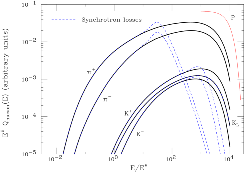
Figure 10: Energy distributions (in the form $Q_{j}(E)\,E^{2}$ versus $E$) for different secondary particles ($\pi^{\pm}$, $K^{\pm}$, $K_{L}$) produced by the $p\gamma$ interactions of relativistic protons in a GRB radiation field. The shape of the primary proton spectrum is also shown (in the form $N_{p}(E)\,E^{2}$ versus $E$) as a thin solid line. The energy spectrum of the isotropic target photons has the form (63). All energies are in units of the characteristic energy $E^{*}$ (defined in equation (72)). The dashed lines are the distributions of the meson energy at decay assuming the presence of magnetic field with value $B=2.78\times 10^{3}~{}(\varepsilon_{\rm b}/{\rm KeV})$ Gauss.

As an intermediate step toward the calculation of the neutrino fluxes we show in fig. 10 the yields of different mesons. The meson yields are calculated for a proton spectrum with exponent $\alpha=2$, and a radiation field with slopes (below and above the break energy) $\beta_{1}=1$ and $\beta_{2}=2$. The solid lines in fig. 10 show the energy distributions of the different mesons at the moment of their creation. In the absence of significant energy losses the curves also describe the energy distributions at decay. One can see that all possible mesons are produced, but with different abundances. The most abundant particles are charged pions, reflecting the fact that a large fraction of the $p\gamma$ interactions happens close to threshold where only single (neutral or positive) pion production is possible. The production of $\pi^{-}$ becomes possible only above the threshold for two pion production, and is therefore suppressed. The production of kaons is significantly smaller, because it is suppressed both dynamically (since it requires the creation of $s\overline{s}$ pairs) and kinematically (because of the larger strange hadron masses). The threshold for the production of mesons containing a strange antiquark $\overline{s}$ ($K^{+}$ and $K^{\circ}$) is lower, since it corresponds to final states containing a strange baryon (such as $\Lambda\,K^{+}$). The production of mesons containing a strange quark $s$ ($K^{-}$ and $\overline{K}^{\circ}$) has a higher threshold since the final state must contain a minimum of two kaons (as for example: $pK^{+}K^{-}$). Accordingly one finds that the productions of different kaon types is ordered as follows: $K^{+}>K_{L}>K^{-}$. The shapes of energy spectra of the mesons are never well approximated by a simple power law, but are always “curving” in a log–log representation. The shapes of these spectra reflect the energy dependence of the proton interaction rate, and the opening up of the different kinematical channels. At the highest energy the rapid drop in the meson yields is connected to the cutoff in the primary proton energy at $E_{\rm max}/E^{*}\sim 10^{4}$. Note that the ratio $\pi^{-}/\pi^{+}$ and $K/\pi$ are not constant but increase with energy reflecting the increasing importance of $\pi^{-}$ and kaon production with growing c.m. energy.

The dashed lines in fig. 10 describe the decay energy distributions of the produced mesons assuming the presence of a magnetic field that corresponds to $\epsilon_{\mu}=3$ (or $B=2.8\times 10^{3}~{}\varepsilon_{\rm b}^{\rm KeV}$ Gauss). Pions created with energy above their critical energy for synchrotron losses (in units of $E^{*}$: $\epsilon_{\pi}\simeq 18.4\epsilon_{\mu}\simeq 55$) lose most of their energy before decay, and therefore the number of pions decaying above this critical energy is strongly suppressed ($\propto(E_{\pi}/\epsilon_{\pi})^{-2}$). One can also notice that synchrotron losses result in an enhancement of the number of pions decaying with energy just below $\epsilon_{\pi}$. This is a pile–up effect due to the fact that all high energy pions (with $E_{\pi}\gg\epsilon_{\pi}$) decay with similar energy distributions. The same effects are present also for charged kaons at higher energy, because the synchrotron energy for charged kaons (in unit of $E^{*}$) is $\epsilon_{K}\simeq 628\epsilon_{\mu}\simeq 34\epsilon_{\pi}\simeq 1900$.

Secondary neutrons are also produced in $p\gamma$ interactions. Assuming that they can freely exit from the source, the $\overline{\nu}_{e}$ spectra from their decay have been calculated and included in the following figures.

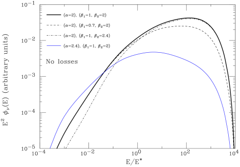
Figure 11: Neutrino energy spectrum (summed over all flavors) from a GRB source, according to the model Waxman-grb . The calculation is performed assuming a proton spectrum $N_{p}(E)\propto E^{-\alpha}$, traveling in an isotropic radiation field of form (63). The different curves are obtained varying the exponent $\alpha$ of the proton spectrum, or the exponents $\beta_{1}$ and $\beta_{2}$ of the radiation field. All energies are measured as fraction of $E^{*}=m_{p}\,\epsilon_{\rm th}/(2\varepsilon_{\rm b})$. The energy losses of all secondary particles are assumed to be negligible.

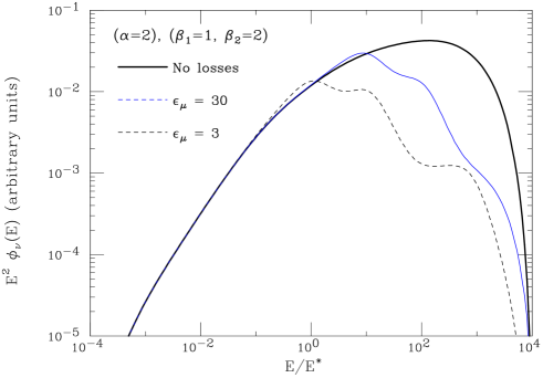
Figure 12: Neutrino energy spectrum (summed over all flavors) from a GRB source (see text). The primary proton spectrum has slope $\alpha=2$, while the target photons have a broken power law energy distribution (see equation (63)) with slopes $\beta_{1}=1$ and $\beta_{2}=2$ below and above the break energy $\varepsilon_{\rm b}$. The curves are calculated assuming different values for the magnetic field, corresponding to values of the critical energy for muons $\epsilon_{\mu}=\infty$, 30 and 3 (see eq. (74)).

Some examples of the resulting neutrino fluxes obtained summing over all possible parent particles and all $\nu$ types are shown in fig. 11 and fig. 12. The lines in fig. 11 are calculated assuming that energy losses for secondary particles are negligible. The different curves correspond to different assumptions about the shape of the energy spectra for the primary protons and target photons. The thick solid curve is calculated with the choice of slopes (for the proton flux and for the radiation field below and above the break energy): $\{\alpha,\beta_{1},\beta_{2}\}=\{2,1,2\}$. The other three curves show the effect of changing the slopes one by one. The largest effect is related to the slope of the primary protons, increasing $\alpha$ from 2 to 2.4 results in an important softening of the neutrino spectrum. The modification of the shape of the energy distribution of the target photons also distorts the neutrino spectrum. Changing the slope below (above) the break energy, modifies the high (low) energy part of the neutrino spectrum. This is easily understood, since high (low) energy neutrinos are produced by higher (lower) energy protons that mostly interact with lower (higher) energy photons. Note that (reflecting the spectra of the parent pions and kaons) the neutrino energy distribution changes gradually its slope and cannot be well fitted by a power law.

Figure 12 illustrates the effect of including synchrotron losses on the neutrino fluxes. The different lines in fig. 12 show the neutrino flux (summed over all $\nu$ types) calculated with the slopes $\{\alpha,\beta_{1},\beta_{2}\}=\{2,1,2\}$, and three different assumptions for the magnetic field that correspond to muon synchrotron energy $\epsilon_{\mu}=\infty$, 30 and 3 (the first case corresponds to negligible losses). Increasing the magnetic field (reducing $\epsilon_{\mu}$) suppresses the neutrino flux at high energy. In general, in the presence of a strong magnetic field in the source, one can identify four interesting neutrino energy ranges, that are related to the ordering of the synchrotron critical energies for different particles: $\epsilon_{\mu}<\epsilon_{\pi}<\epsilon_{K}$. At sufficiently low energies the synchrotron losses are completely negligible; at higher energy the muons energy losses have to be taken into account; at still higher energy also the losses of charged pions must be considered; at the highest energy the emission of synchrotron radiation is important also for charged kaons. In general, in the presence of important synchrotron emission, one can have some pile–up effects, due to the fact that all high energy particles decay just below their critical synchrotron energy.

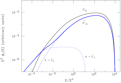
Figure 13: Energy spectra for $\nu_{e}$ and $\overline{\nu}_{e}$ from a GRB source (proton slope $\alpha=2$, target photon slopes $\beta_{1}=1$ and $\beta_{2}=2$, no magnetic field) For the $\overline{\nu}_{e}$ flux also the contributions from meson and neutron decay are separately shown. Neutron decay dominates at low energy.

The inclusive neutrino spectra shown in the previous figures contain the contribution of the $\overline{\nu}_{e}$ from $n$ decay. The structure of this contribution is illustrated in fig. 13. The anti–neutrinos from neutron decay have significantly lower energies that the neutrinos from meson decay. They are the main component of the neutrino flux at the lowest energies, where however they are difficult to observe because the flux is suppressed and the cross section is small.

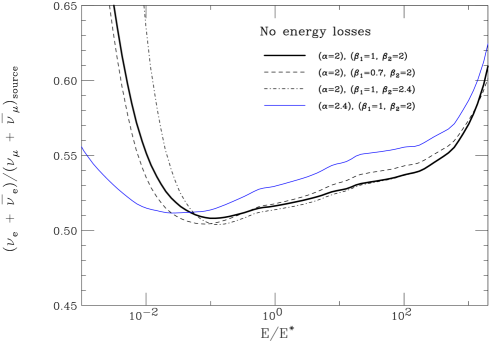
Figure 14: Ratio $(\nu_{\mu}+\overline{\nu}_{\mu})/(\nu_{e}+\overline{\nu}_{e})$ for neutrinos from a GRB source. The ratio correspond to the spectra shown in fig. 11. The rapid increase at low energy is due to the effect of $\overline{\nu}_{e}$ from $n$ decay.

The flavor ratios $R_{e\mu}=(\nu_{e}+\overline{\nu}_{e})/(\nu_{\mu}+\overline{\nu}_{\mu})$ that correspond to the neutrino spectra of the previous figures are shown in figures 14 and 15. The flavor ratio is energy and model dependent. The $R_{e\mu}$ ratios shown in figure 14 correspond the energy spectra of fig. 11 and are calculated assuming that all energy losses are negligible. At the lowest energy the ratio $R_{e\mu}$ increases rapidly due to the contribution of $\overline{\nu}_{e}$ from $n$ decay. At higher energy the ratio $R_{e\mu}$ stays close to the value of 1/2, however the expanded scale allows to see that the “naive” result is not exact. The value of $R_{e\mu}$, for the reasons illustrated in section V, are correlated with the shape of the energy spectrum. The gradual softening of the neutrino energy distribution with growing $E_{\nu}$ is reflected in a slow increase of $R_{e\mu}$. Comparing the different curves, one can also see that the curve calculated for $\alpha=2.4$ that gives the softest neutrino spectrum correspond (at sufficiently high energy) to the highest $R_{e\mu}$.

The effects of the existence of significant synchrotron losses are very important for the flavor ratio. The main effect is the effective loss of the neutrinos from high energy muon decay. This results in a “pile–up” effects that produced an increase in the ratio for neutrino energies below the synchrotron muon energy $\epsilon_{\mu}$. Above this energy the ratio falls steeply reflecting the effective absence of the main source (muon decay) of electron neutrinos. The flavor ratio however does not vanish because kaons have decay modes into electron neutrinos, and reaches a level of a few percent. At very large energy the role of neutral kaons (that do not suffer synchrotron losses) become enhanced and the flavor ratio grows because of the importance of the $K^{\circ}_{e3}$ decay mode.

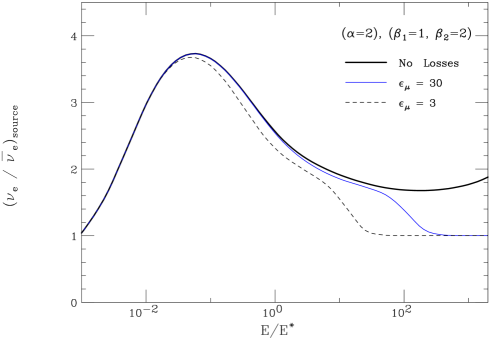
Figure 16: Ratio $(\nu_{e}/\overline{\nu}_{e})$ at the source for neutrinos from a GRB source. The ratio correspond to the spectra shown in fig. 12. At low energy the ratio is low because of the importance of $\overline{\nu}_{e}$ from $n$ decay. At higher energy the ratio decreases because of the increased importance of $\pi^{-}$ production. For high magnetic field, at high energy the dominant source of $\nu_{e}$ and $\overline{\nu}_{e}$ becomes $K_{L}$ decay, and the $(\nu_{e}/\overline{\nu}_{e})$ ratio becomes unity.

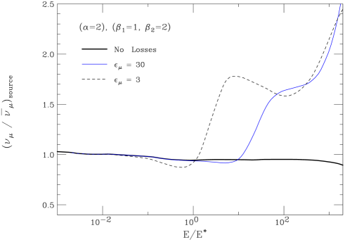
Figure 17: Ratio $(\nu_{\mu}/\overline{\nu}_{\mu})$ at the source for neutrinos from a GRB source. The ratio correspond to the spectra shown in fig. 12. The three curves correspond to three different values of the magnetic field in the source. At low energy (and at all energies for small $B$) the ratio is unity, reflecting the fact that the chain decay of a charged pion produces a $\nu_{\mu}$ and a $\overline{\nu}_{\mu}$. In the presence of a large magnetic field, the neutrinos from muon decay are suppressed, and the flavor ratio is determined by the $\pi^{+}/\pi^{-}$ ratio. At the highest energies charged kaon decay becomes the dominant source of $\nu_{\mu}$ and $\overline{\nu}_{\mu}$ and the flavor ratio reflects the $K^{+}/K^{-}$ ratio.

Figure 16 and figure 17 show the neutrino/anti–neutrino ratios $\nu_{e}/\overline{\nu}_{e}$ and $\nu_{\mu}/\overline{\nu}_{\mu}$ calculated for the same three situations present in fig. 12 and 15 (that is slopes $\{\alpha,\beta_{1},\beta_{2}\}=\{2,1,2\}$ and three values of the magnetic field that corresponds to $\epsilon_{\mu}=\infty$, 30 and 3).

The $\nu/\overline{\nu}$ ratios are difficult to measure because the detectors have no capability to measure the charge of the final state charged lepton in charged current neutrino interactions. The most attractive idea Anchordoqui:2004eb to estimate the $\nu_{e}/\overline{\nu}_{e}$ ratio is the comparison of the event rate at and near the “Glashow resonance” glashow at $E_{\nu}\sim M_{W}^{2}/(2\,m_{e})$. The resonance is present only for $\overline{\nu}_{e}$ in reactions such as $\overline{\nu}_{e}+e^{-}\to{\rm hadrons}$ that can proceed via the formation of a $W^{-}$ boson in the $s$ channel, while non–resonant events proceed via the normal charged current interaction on nucleons.

The study of $\nu_{e}/\overline{\nu}_{e}$ ratio is particularly interesting because it has been proposed Anchordoqui:2004eb as a method to distinguish $pp$ and $p\gamma$ interactions as the source of the neutrinos. The idea is that the $\nu_{e}/\overline{\nu}_{e}$ ratio at the source is close to unity for a $pp$ source, when the interactions produce approximately equal numbers of positive and negative pions (that decay into $\nu_{e}$ and $\overline{\nu}_{e}$), and is very large (or actually diverges) for $p\gamma$ interactions, when most interactions happen close to threshold, and the cross section is dominated by single pion production (via the $\Delta$ resonance), and therefore only $\pi^{+}$ production is present. This argument is qualitatively right, but quantitatively incorrect, in fact as discussed above, in general increasing $E_{p}$ a broader range of c.m. energies becomes possible, and this results in a growing contribution of negative pions to neutrino production. In certain circumstances also the contribution of kaons can become important. This is illustrated in fig. 16 that shows the $\nu_{e}/\overline{\nu}_{e}$ ratio. At the lowest energies the flux is dominated by the $\overline{\nu}_{e}$ from $n$ decay, and the $\nu_{e}/\overline{\nu}_{e}$ ratio is therefore small. When the contribution of neutrinos from pion decay becomes dominant the ratio $\nu_{e}/\overline{\nu}_{e}$ is significantly larger than one, because positive pions are more abundantly produced than negative ones. In fact below the threshold for two pion production the ratio $\pi^{+}/\pi^{-}$ diverges. With growing energy the ratio $\pi^{+}/\pi^{-}$ decreases because of the growing importance of multiple pion production. This is reflected in a decrease of the $\nu_{e}/\overline{\nu}_{e}$ ratio that at large energies becomes $\sim 2$. If a large magnetic field is present, at large energy the synchrotron energy losses for muons become important and neutrinos from muon decay are suppressed. The decay of neutral kaons ($K_{L}$) becomes the dominant source of $\nu_{e}$ and $\overline{\nu}_{e}$, and the ratio $\nu_{e}/\overline{\nu}_{e}$ becomes unity.

The ratio $\nu_{\mu}/\overline{\nu}_{\mu}$ (shown in fig. 17) is approximately unity at low energy, reflecting the fact that each charged pion, after chain decay, contributes a $\nu_{\mu}$ and a $\overline{\nu}_{\mu}$. The existence of important synchrotron losses can modify this quite robust prediction. At high energy, when muons energy losses become significant, only the neutrinos from direct pion decay are important, and the ratio $\nu_{\mu}/\overline{\nu}_{\mu}$ is approximately equal to the $\pi^{+}/\pi^{-}$. At larger energy, charged kaons become the dominant $\nu_{\mu}$ and $\overline{\nu}_{\mu}$ source and the $\nu_{\mu}/\overline{\nu}_{\mu}$ ratio increases reflecting the higher $K^{+}/K^{-}$ ratio.

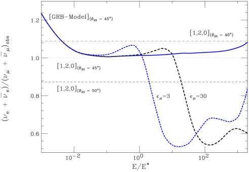
Figure 18: Observable ratio $(\nu_{\mu}+\overline{\nu}_{\mu})/(\nu_{e}+\overline{\nu}_{e})$ after propagation for the neutrinos from a GRB source. The solid lines corresponds to the source models shown in fig. 12, and 15. The three curves differ for the value of the magnetic field that corresponds to $\epsilon_{\mu}=3$, 30 and $\infty$ (no field). The neutrino oscillation parameters have been chosen as $\theta_{23}=45^{\circ}$, $\theta_{12}=34^{\circ}$ and $\theta_{13}=0$. The thin dotted are calculate for the “naive” assumption of a source composition $[\nu_{e},\nu_{\mu},\nu_{\tau}]=[1,2,0]$. The dotted line assumes the same mixing parameters as above. The Dashes (dot–dashed) line has $\theta_{23}=50^{\circ}$ ( $40^{\circ}$).

In fig. 18 we show the $(\nu_{e}/\nu_{\mu})$ ratio for an Earth observer. To propagate neutrino we have used standard oscillations with mixing parameters $\theta_{23}=45^{\circ}$, $\theta_{12}=34^{\circ}$ and $\theta_{13}=0$. In the figure we have also shown the same observable ratio for a source with the “naive” composition $[\nu_{e},\nu_{\mu},\nu_{\tau}]=[1,2,0]$. For the “best fit” values of the mixing parameters the observable $(\nu_{e}/\nu_{\mu})$ has the well known value of unity. Changing the value of the $\theta_{23}$ angle by $\pm 5^{\circ}$ the ratio changes by $-13\%$ ($+7\%$). Similarly for $\theta_{13}=5^{\circ}$ the ratio take values in the interval (0.95,1.04) depending on the value of the phase $\delta$. This figure illustrates the interplay between astrophysical and particle physics uncertainties (also shown before in equations (3), (4) and (5)). In order to perform a measurement of $\theta_{23}$ one clearly needs an accurate control of the initial flux composition.

The description of the emission of neutrinos from GRB that we have used in this section following reference Waxman-grb is very simplified, and could be improved in many aspects. The results of our calculation show that one obtains non trivial and intriguing energy dependences of the flavor ratios, that could reveal important informations about the source. This qualitative observation is of a much more general validity and one expects that in most cases, and also using more realistic descriptions of the sources, one should find non trivial structures in the energy spectra and flavor composition of the astrophysical neutrino signals.

IX Experimental Flavor identification

In this work we will not consider in detail the crucial problem of the experimental determination of the flavor ratios. Several experimental approaches for the detection are at present being developed. The concept that is in the most advanced stage is a large volume (cubic Kilometer) ice or water Cherenkov detector, with photon detectors distributed inside the volume, as originally proposed by the Dumand group Dumand and now in different stages of development at the South Pole Amanda ; IceCube , in the Baikal lake Baikal and in the mediterranean sea Nestor ; Antares ; Nemo . Several other alternative techiques are also being developed Learned:2003 , that includes radio Rice ; Anita , acoustic and air shower Letessier-Selvon ; euso-nu detection methods.

A very imporant problem is of course the amount of data that is required in order to reduce the statistical errors to the level needed for a meaningful measurement. Today we only have upper limits for the astrophysical neutrino fluxes, optimistically one can expect that these fluxes will be soon discovered just below the current upper limits, however even in this case the event rates will remain small, and one will need very long data taking periods, or much larger mass detectors to collect sufficient data vissani ; meloni .

In this section we want to stress the point that in all the experimental methods that are envisaged, the measurement of the flavor ratio is connected with a determination of (or a theoretical assumption on) the shape of the energy distribution of the neutrino fluxes. This happens because the detection methods of different neutrino flavors have efficiencies with different dependences on $E_{\nu}$. If the statistical errors are sufficiently small (with very large mass detectors), and having achieved perfect control of the detector acceptances and efficiencies, the uncertainties in the determination of the neutrino spectral shapes will remain as the dominant source of error in the measurement of the flavor ratios.

To illustrate the interplay between the spectral shapes and the determination of the flavor ratio one can consider the case of the Km³ type Cherenkov telescopes. In these detectors one expects to find different classes of neutrino induced events Beacom-flavor .

• In “Track Events” a single up–going muon is seen entering the detector. The energy of the muons can be estimated from the amount of Cherenkov light produced by the photons and $e^{\mp}$ pairs radiated from the muon track.

• In “Shower Events” one observes the release of a large amount of Cherenkov light generated by the shower induced by a neutrino interaction in the detector volume. The amount of light can be translated in the estimate of a visible energy release $E_{\rm vis}$.

• In “Double Bang Events” double-bang ; Fargion:1997eg one detects two distinct energy releases inside the detector volume, with space and time separations that are consistent with the propagation and decay of an energetic tau lepton.

Events in class (i) are associated with the charged current (CC) interactions of muon neutrinos below the detector. Events in class (ii) can be produced by several types of neutrino interactions. Electron (anti)neutrino CC interactions are the main source of shower events, there are also contributions from the neutral current interactions of all neutrino types, and in general also from the CC interactions of $\nu_{\mu}$ and $\nu_{\tau}$. Finally events in class (iii) are generated by $\nu_{\tau}$ CC interactions. Clearly, the ratio of the frequencies of these three classes of events does give information about the flavor composition of the neutrino fluxes. In fact the ratio of the event rates for “Shower” and “Tracks” events has been proposed as the best method for a measurement of the $\nu_{e}/\nu_{\mu}$ flavor ratio.

The frequency of “Track” events can be studied as a function of the visible muon energy $E_{\mu}$. The differential event rate can be calculated as:

$$\frac{dN_{\rm Tracks}}{dE_{\mu}\;d\Omega_{\oplus}\;dt}(E_{\mu},\Omega_{\oplus})=A_{\rm det}^{\rm Tracks}(E_{\mu},\Omega_{\oplus})~{}\sum_{\nu_{\mu},\overline{\nu}_{\mu}}~{}\int dE_{\nu}~{}\phi_{\nu}(E_{\nu},\Omega_{\oplus})~{}\frac{dY_{\nu\to\mu}}{dE_{\mu}}(E_{\mu};~{}E_{\nu})$$ (75)

where $A_{\rm det}^{\rm Tracks}(E_{\mu},\Omega_{\oplus})$ is the detector effective area for the detection of muons with energy $E_{\mu}$ from the direction $\Omega_{\oplus}$, $dY_{\nu\to\mu}/dE_{\mu}(E_{\mu};~{}E_{\nu})$ is the “muon yield”, that is the probability that a $\nu_{\mu}$ ($\overline{\nu}_{\mu}$) of energy $E_{\nu}$ produces a $\mu^{\mp}$ of energy $E_{\mu}$ at the detector. In this equation we have assumed that the muon and the neutrino are collinear. Even for an individual source, the energy spectrum will depend on the zenith angle $\theta_{\oplus}$, because of the effects of neutrino absorption in the Earth. This procedure hower implies a good understanding of the neutrino energy spectrum.

The rate of “Shower” events with a visible energy release $E_{\rm vis}$ can be estimated as the convolution

$$\frac{dN_{\rm Showers}}{dE_{\rm vis}\;d\Omega_{\oplus}\;dt}(E_{\rm vis},\Omega_{\oplus}) \simeq \frac{M_{\rm det}(E_{\rm vis})}{m_{p}}~{}\Big{\{}\sum_{\nu_{e},\overline{\nu}_{e}}\left[\phi_{\nu}(E_{\nu},\Omega_{\oplus})~{}\sigma_{\nu}^{\rm cc}(E_{\nu})\right]_{E_{\nu}\simeq E_{\rm vis}}$$ (76)

$$+ \sum_{{\rm All}~{}\nu}\int dE_{\nu}~{}\phi_{\nu}(E_{\nu},\Omega_{\oplus})\int_{0}^{1}dy~{}\frac{d\sigma_{\nu}^{\rm nc}}{dy}(y,E_{\nu})\;\delta[E_{\rm vis}-E_{\nu}\,y]~{}~{}~{}~{}~{}$$

$$+ \left[(\nu_{\mu},~{}\overline{\nu}_{\mu})~{}{\rm CC}\right]+\left[(\nu_{\tau},~{}\overline{\nu}_{\tau})~{}{\rm CC}\right]~{}~{}\Big{\}}~{}.$$

In this equation $M_{\rm det}(E_{\rm vis})$ is the effective detector mass; the first line is the contribution from the charged current interactions of electron (anti)–neutrinos, in this case the visible energy, in first approximation (neglecting differences in the light to energy conversion for e.m. and hadronic showers) equals the initial $\nu$ energy; the second line is the contribution from neutral current interactions, in this case the visible energy is only a fraction of the initial energy because the neutrino in the final state carries away an invisible energy $E_{\nu}\,(1-y)$. The contributions of $\nu_{\mu}$ and $\nu_{\tau}$ CC interactions to the shower event rate in (76) has been left implicit. A fraction of these interactions can probably be identified and eliminated selecting events with a muon in the final state, or a double bang structure, but the rest will contribute to the “shower” class of events.

From (75) and (76) it is clear that the energy response for the two classes of events is different, with the “Track” events selecting larger $E_{\nu}$. Therefore the ratio for the integral rates for “Shower” and “Tracks” events is strongly dependent on the spectral shape of the fluxes. Use of the differential distributions in $E_{\mu}$ and $E_{\rm vis}$ allows in principle to unfold the shape of the neutrino energy spectra, however an important difficulty is that a narrow interval in the muon energy $E_{\mu}$ (that can however be measured only with modest resolution) corresponds to a very broad interval in $E_{\nu}$. Also $E_{\rm vis}$ in shower events is not in a one to one correspondence with $E_{\nu}$. The unfolding procedure has therefore some significant limitations.

As an illustration of these problems, one can look back at the original discovery of neutrino oscillations Kamiokande ; IMB ; SK with atmospheric neutrinos. The evidence collected by the SK SK experiment for subGeV fully contained events ($E_{\rm vis}\leq 1.33$ GeV) implied comparing the ratio of the observed rates of $e$–like and $\mu$–like events with a MC prediction $(\mu/e)_{\rm MC}\simeq 1.50$. This prediction is significantly smaller than the no–oscillation ratio $(\nu_{\mu}+\overline{\nu}_{\mu})/(\nu_{e}+\overline{\nu}_{e})\simeq 2$ for the combination of several reasons, related to the difference in detector acceptances for $e$–like and $\mu$–like events. The experimental cuts select for the $e$–like events a broader energy range, both at the low and high energy ends (at low energy because electrons have a larger yield of Cherenkov photons, and at high energy because electrons have a shorter range and are more easily contained). For this reason the MC prediction does depend on the shape of the neutrino fluxes. For these sub–GeV events, the intervals of $E_{\nu}$ for the two classes of $e$–like and $\mu$–like events are very similar, and therefore the associated systematic uncertainty in the $(\mu/e)$ prediction is relatively small, but it remains as a relevant source of error.

The comparison of the rates of classes of events that correspond to very different atmospheric neutrino energy, such as samples of fully contained $e$–like events and upgoing muons (that are produced by $\nu_{\mu}$ charged current interaction with a median energy of order 100 GeV) also allows in principle to verify the existence of $\nu_{\mu}\leftrightarrow\nu_{\tau}$ transitions. However in this case the systematic uncertainty in the prediction of the shape of the energy distribution is much larger, and in practice this method gives only marginal evidence for the existence of a suppression of the upgoing muon rate.

In conclusion, the extraction of the $e/\mu$ flavor ratio from the comparison of the rates of “Track” and “Shower” events in high energy neutrino telescopes requires excellent control of the detector performances, and a sufficiently precise knowledge of the shapes of the neutrino spectra. The determination of these shapes could be obtained from the data themselves (the “unfolding method”) or with the help of reliable theoretical models for the source. In both cases the task appears as remarkably difficult.

X Conclusions

The study of astrophysical neutrinos can be used for two distinct goals: the understanding of their sources and the investigations of the neutrino properties. These two goals are in a sense contradictory. The investigation of the neutrino fundamental properties requires a comparison of the observations with expectations that must necessarily be based on a sufficiently accurate understanding of the source. On the other hand the flavor composition of a neutrino signal encodes information about the source properties, but in order to extract this information one needs to know the properties of flavor transitions over galactic or cosmological distances with sufficient accuracy.

Several recent works Pakvasa:2004hu ; Beacom-flavor ; Barenboim:2003jm have speculated that it is possible to discovery new neutrino properties, or even measure precisely the parameters of the already established standard oscillations astro-standard from the observation of future astrophysical neutrino sources assuming that the flavor ratios at the source are robustly predictable. The often repeated argument is that a “standard neutrino source” is dominated by charged pion decay, and therefore emits the different flavors (summing over $\nu$ and $\overline{\nu}$) with relative intensities: [$\nu_{e},\nu_{\mu},\nu_{\tau}]\simeq[1,2,0]$. This statement however must be understood as a first approximation of only limited validity. First of all it requires that the energy losses of the muons created in charged pion decay are negligible. This crucial assumption is satisfied for several but not all of the proposed neutrino sources. Even for “thin environment sources” (where the density of ordinary matter and magnetic field is sufficiently low so that the energy losses for all secondary unstable particles can be safely neglected) the flavor ratios are (slowly varying) functions of the neutrino energy, with values that are determined by the shape of the neutrino spectra and by the nature of target material. This dependence arises from two effects: the first is that in general the contributions of other weakly decaying particles (kaons and in some cases also neutrons) is not negligible, the second is that, even if charged pions are the only significant neutrino source, the three neutrinos that are emitted in a $\pi^{\pm}$ chain decay have different energy spectra. Folding these decay spectra with the energy distribution of the parent particles, one obtains slightly different shapes, and therefore energy dependent flavor ratios. In the special case where the parent pion spectrum is a power law, the neutrino energy distributions have also a power law form with the same slope, and the $\nu$ flavor ratios are constants. As a (phenomenologically important) example, the neutrino fluxes with spectrum $\propto E_{\nu}^{-2}$ emerging from a “thin”, charged pion source, have relative intensity (at the source) [$\nu_{e},\nu_{\mu},\nu_{\tau}]\simeq[1,1.86,0]$, a 7% deviation from the naive expectation.

In general, the combined effects of different shapes for the $\nu$ energy spectra, and different contributions of the relevant weakly decaying particles correspond to variations of order 10% of the $\nu_{e}/\nu_{\mu}$ ratio (in some special circumstances even larger). The size of these corrections is however comparable to the effects on the observable flavor ratios due to the present uncertainties in the values of the standard oscillation parameters (for a quantitative illustration of this point see equations (3), (4) and (5)). The very ambitious program astro-standard to attempt a precision measurement of $\theta_{23}$ or a determination of $\theta_{13}$ with astrophysical neutrinos cannot therefore ignore these problems, and requires a very precise control of the structure and properties of the neutrino sources.

Much larger effects on the neutrino flavor ratio arise from situations where the environment of the source contains large energy densities in magnetic field, or in ordinary matter. In the presence of sufficiently large magnetic fields, such as those that could exist in a GRB fireball, high energy muons can lose most of their energy to synchrotron radiation Rachen:1998fd ; Kashti and their contribution to the neutrino fluxes becomes strongly suppressed. This results in a very small $\nu_{e}/\nu_{\mu}$ ratio, with a value determined by the size of the kaon contribution (that generate electron neutrinos in direct decay modes). At higher energy also pions suffer important synchrotron losses, and kaon decay become the dominant $\nu$ source for all flavors. In some extreme circumstances neutral kaon decay will remain as the only significant neutrino source with a $\nu_{e}/\nu_{\mu}$ ratio at the source of order unity.

In some circumstances it is possible that interactions with ordinary matter play a major rôle. If the density is sufficiently large high energy pions reinteract before decaying. This supresses the neutrino fluxes and enhances the contribution of kaon decay. Summing over charged and neutral kaons, this also results in a significantly reduced $\nu_{e}/\nu_{\mu}$ ratio.

The prediction of the neutrino flavor ratios in these circumstances (strong magnetic field or large densities of ordinary matter) is going to be very difficult, because the assumption of a “single volume” homogeneous source is very likely a poor (and in any case not demonstrable) assumption. The neutrinos will likely emerge with different spectra and flavor ratios from different regions of the source, and for example fitting the data including a value of the field $B$, and/or a matter density $n_{\rm gas}$ is likely to be only a poor approximation.

The existence of neutrino sources dominated by neutron decay are also a theoretical possibility, in situations where photodisintegration of relativistic nuclei interacting on a radiation field is possible while pion photoproduction is kinematically forbidden. If such sources exist, it will however be very difficult to use these fluxes for studies of the neutrino flavor transitions because in general one expect them to have an important “contamination” of muon neutrinos in their initial flavor composition. In fact it is unnatural to have the pion photoproduction to be absolutely forbidden, because the energy thresholds for nuclear photodisintegration and pion production differ only by one order of magnitude. The size of the contribution of pion decay to the neutrino fluxes in these circumstances is difficult to control.

Even considering all the caveats of our discussion, there are some circumstances where observations of astrophysical neutrinos could lead to the discovery that new physics is involved in the propagation of neutrinos over astrophysical distances. In particular the investigation of the existence of neutrino decay nu-decay is a very attractive possibility. The observation of the absence (or very strong suppression) of a $\nu_{e}$ component in the measured fluxes cannot be explained with even extreme variations of the source astrophysical properties, and is on the contrary predicted (for any type of source) in a neutrino decay model with inverse mass hierarchy. For the normal mass hierarchy the neutrino decay model predicts a large $(\nu_{e}/\nu_{\mu})_{\rm obs}$ ratio between 3 and 6. If the neutrinos have standard properties, ratios $(\nu_{e}/\nu_{\mu})_{\rm obs}$ much larger than unity are only possible (and limited to $\lesssim 4$) for sources dominated by $\nu_{e}$ emission. Therefore from the observation of a large $(\nu_{e}/\nu_{\mu})_{\rm obs}$ ratio it could be possible to infer the existence of $\nu$ decay in the normal mass hierarchy case. This could require some understanding of the properties of the $\nu$ source.

In the general case the observation of flavor ratios very different from the “standard source” values (relative intensities $[\nu_{e},\nu_{\mu},\nu_{\tau}]_{\rm obs}\sim[1,1,1]$) could be interpreted as evidence for some form of new physics in neutrino propagation, but also, and probably more economically, as an indication of the existence of some unexpected properties in the $\nu$ source. Resolving these ambiguities is in principle possible, but certainly not easy, and requires a careful interpretation of the multi–messenger (photons, neutrinos and possibly cosmic rays) and multi–wavelength observations.

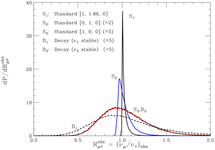
Figure 2: Distribution of the observable flavor ratio $R_{\mu\tau}=(\nu_{\mu}/\nu_{\tau})_{\rm obs}$ (see caption of fig. 1). Some of the curves have been renormalized for an easier observation of their shape.

Figure 8: Proton interaction rate in a radiation field of the form (63). The energy $E^{*}$ (defined in equation (72)) corresponds to the threshold proton energy for interaction with photons with energy $\varepsilon_{\rm b}$. The dashed line neglects the interactions with all photons with energy $\varepsilon>\varepsilon_{\rm b}$.

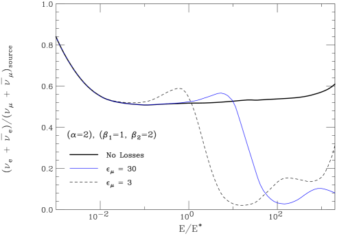
Figure 15: Ratio $(\nu_{\mu}+\overline{\nu}_{\mu})/(\nu_{e}+\overline{\nu}_{e})$ for neutrinos from a GRB source. The ratio correspond to the spectra shown in fig. 12. The three curves are calculated assuming different values of the magnetic field in the source (and proton slope $\alpha=2$, target photon slopes $\beta_{1}=1$ and $\beta_{2}=2$). The decrease of the flavor ratio at high energy for large $B$ is associated to the important synchrotron losses of high energy muons.

References

- (1) T. K. Gaisser, F. Halzen and T. Stanev, Phys. Rept. 258, 173 (1995) [Erratum-ibid. 271, 355 (1996)];
- (2) J. G. Learned and K. Mannheim, Ann. Rev. Nucl. Part. Sci. 50, 679 (2000); F. Halzen and D. Hooper, Rept. Prog. Phys. 65, 1025 (2002);
- (3) P. Lipari, Nucl. Instrum. Meth. A 567, 405 (2006) [astro-ph/0605535].
- (4) EGRET Collaboration, Astrophys. J. Suppl. 123, 79 (1999).
- (5) HESS Collaboration, Science 307, 1938 (2005) [astro-ph/0504380]. HESS Collaboration, Astrophys. J. 636, 777 (2006) [astro-ph/0510397].
- (6) K.S. Hirata, et al., Phys. Lett. B 205 416 (1988); Phys. Lett. B280 146 (1992).
- (7) IMB Coll., Casper et al., Phys. Rev. Lett. 66 2561 (1991); Phys. Rev. D46 3720 (1992).
- (8) J. G. Learned and S. Pakvasa, Astropart. Phys. 3, 267 (1995).
- (9) H. Athar, M. Jezabek and O. Yasuda, Phys. Rev. D 62, 103007 (2000) [hep-ph/0005104].
- (10) D. V. Ahluwalia, Mod. Phys. Lett. A 16, 917 (2001) [hep-ph/0104316].
- (11) S. Pakvasa, Mod. Phys. Lett. A 19, 1163 (2004) [Yad. Fiz. 67, 1179 (2004)] [hep-ph/0405179].
- (12) G. Barenboim and C. Quigg, Phys. Rev. D 67, 073024 (2003) [hep-ph/0301220].
- (13) J. F. Beacom, N. F. Bell, D. Hooper, S. Pakvasa and T. J. Weiler, Phys. Rev. D 68, 093005 (2003) [Erratum-ibid. D 72, 019901 (2005)] [hep-ph/0307025].
- (14) Y. Chikashige, R. N. Mohapatra and R. D. Peccei, Phys. Rev. Lett. 45, 1926 (1980). G. B. Gelmini and M. Roncadelli, Phys. Lett. B 99, 411 (1981);
- (15) A. Acker, S. Pakvasa and J. T. Pantaleone, Phys. Rev. D 45, 1 (1992).
- (16) J. F. Beacom, N. F. Bell, D. Hooper, S. Pakvasa and T. J. Weiler, Phys. Rev. Lett. 90, 181301 (2003) [hep-ph/0211305].
- (17) L. Wolfenstein, Nucl. Phys. B 186, 147 (1981); S. T. Petcov, Phys. Lett. B 110, 245 (1982); S. M. Bilenky and B. Pontecorvo, Sov. J. Nucl. Phys. 38, 248 (1983); C. Giunti, C. W. Kim and U. W. Lee, Phys. Rev. D 46, 3034 (1992); M. Kobayashi and C. S. Lim, Phys. Rev. D 64, 013003 (2001). K. R. Balaji, A. Kalliomaki and J. Maalampi, Phys. Lett. B 524, 153 (2002).
- (18) J. F. Beacom, N. F. Bell, D. Hooper, J. G. Learned, S. Pakvasa and T. J. Weiler, Phys. Rev. Lett. 92, 011101 (2004) [hep-ph/0307151].
- (19) P. Keranen, J. Maalampi, M. Myyrylainen and J. Riittinen, Phys. Lett. B 574, 162 (2003) [hep-ph/0307041].
- (20) D. Hooper, D. Morgan and E. Winstanley, Phys. Lett. B 609, 206 (2005) [hep-ph/0410094].
- (21) M. Gasperini, Phys. Rev. D 39, 3606 (1989).
- (22) H. Minakata and A. Y. Smirnov, Phys. Rev. D 54, 3698 (1996) [hep-ph/9601311];
- (23) R. Fardon, A. E. Nelson and N. Weiner, JCAP 0410, 005 (2004) [astro-ph/0309800].
- (24) P. Q. Hung and H. Päs, Mod. Phys. Lett. A 20, 1209 (2005) [astro-ph/0311131].
- (25) E. Waxman and J. N. Bahcall, Phys. Rev. Lett. 78, 2292 (1997) [astro-ph/9701231].
- (26) A. Strumia and F. Vissani, Nucl. Phys. B 726, 294 (2005) [hep-ph/0503246].
- (27) P. Lipari, Astropart. Phys. 1, 195 (1993).
- (28) W. M. Yao et al. [Particle Data Group], J. Phys. G 33, 1 (2006).
- (29) T. Kashti and E. Waxman, Phys. Rev. Lett. 95, 181101 (2005) [astro-ph/0507599].
- (30) M. Conversi, E. Pancini and O. Piccioni, Phys. Rev. 71, 209 (1947).
- (31) J. P. Rachen and P. Meszaros, Phys. Rev. D 58, 123005 (1998) [astro-ph/9802280].
- (32) L. A. Anchordoqui, H. Goldberg, F. Halzen and T. J. Weiler, Phys. Lett. B 593, 42 (2004) [astro-ph/0311002].
- (33) T. Piran, Rev. Mod. Phys. 76, 1143 (2004) [astro-ph/0405503].
- (34) B. Zhang and P. Meszaros, Int. J. Mod. Phys. A 19, 2385 (2004) [astro-ph/0311321].
- (35) A. Dar and A. De Rujula, Phys. Rept. 405, 203 (2004) [astro-ph/0308248].
- (36) R.D. Preece et al., Astrophys.J.Suppl.Ser. 126, 19 (2000).
- (37) L. A. Anchordoqui, H. Goldberg, F. Halzen and T. J. Weiler, Phys. Lett. B 621, 18 (2005) [hep-ph/0410003].
- (38) The details of the Montecarlo code will be presented elsewhere.
- (39) S.L. Glashow, Phys. Rev. 118, 316, (1960).
- (40) A. Roberts, Rev. Mod. Phys. 64, 259 (1992);
- (41) E. Andres et al., Nature 410, 441 (2001).
- (42) A. Achterberg et al. [IceCube Collaboration], Astropart. Phys. 26, 155 (2006) [astro-ph/0604450].
- (43) V. Balkanov et al., Astropart. Phys. 14, 61 (2000).
- (44) S. E. Tzamarias, Nucl. Instrum. Meth. A 502, 150 (2003).
- (45) J. A. Aguilar et al. [ANTARES Collaboration], Astropart. Phys. 26, 314 (2006) [astro-ph/0606229].
- (46) F. Ameli, M. Bonori and F. Massa, Eur. Phys. J. C 25, 67 (2002).
- (47) J.Learned, Nucl. Phys. Proc. Suppl. 118 (2003) 405.
- (48) I. Kravchenko et al., Int. J. Mod. Phys. A 21S1, 153 (2006).
- (49) H. Falcke, P. Gorham and R. J. Protheroe, New Astron. Rev. 48, 1487 (2004) [astro-ph/0409229].
- (50) A. Letessier-Selvon, Nucl. Phys. Proc. Suppl. 118, 399 (2003) [astro-ph/0208526].
- (51) Euso Collaboration, Nuovo Cim. 24C (2001) 445.
- (52) F. Vissani, astro-ph/0609575.
- (53) D. Meloni and T. Ohlsson, hep-ph/0612279.
- (54) D. Fargion, astro-ph/9704205.
- (55) Y. Fukuda et al. [Super-Kamiokande Collaboration], Phys. Rev. Lett. 81, 1562 (1998) [hep-ex/9807003].
- (56) P. D. Serpico and M. Kachelriess, Phys. Rev. Lett. 94, 211102 (2005) [hep-ph/0502088]. P. Bhattacharjee and N. Gupta, hep-ph/0501191. W. Winter, Phys. Rev. D 74, 033015 (2006) [hep-ph/0604191]. P. D. Serpico, Phys. Rev. D 73, 047301 (2006) [arXiv:hep-ph/0511313]. W. Rodejohann, JCAP 0701, 029 (2007) [hep-ph/0612047].