Néel order in the two-dimensional $S=\frac{1}{2}$-Heisenberg Model

Abstract

The existence of Néel order in the $S=\frac{1}{2}$ Heisenberg model on the square lattice at $T=0$ is shown using inequalities set up by Kennedy, Lieb and Shastry in combination with high precision Quantum Monte Carlo data.

The ground state order of quantum spin systems, in particular the issue whether the ground state shows long range magnetic order, has attracted long and continuous interest. For the prototype of spin models, the antiferromagnetic Heisenberg model, the existence of Néel order at low temperatures was proved in the seminal paper of Dyson, Lieb and Simon DLS in 1978 for spin $S\geq 1$ and spatial dimension $d\geq 3$ and also for $S=\frac{1}{2}$ and $d>3$.

Ten years later Kennedy, Lieb and Shastry KLS showed that also for $S=\frac{1}{2}$ and $d=3$ Néel order in the ground state exists.

The situation in two dimensions is different and more subtle, since the Mermin-Wagner-Hohenberg theorem forbids Néel order at finite $T$, leaving open however the possibility of Néel order in the ground state. The existence of Néel order for the two-dimensional model and $S\geq 1$ was shown in AKLT ; NP and later in KLS by an independent derivation of the relevant inequality at $T=0$.

However the inequalities sufficient to show Néel order for $S=1$ in the two-dimensional case are not sufficient to construct an analogous proof for $S=\frac{1}{2}$. Thus the case of $S=\frac{1}{2}$ remains an open problem. Still it is possible to derive inequalities concerning spin-spin correlations at short distances KLS which are violated if Néel order is present. That is, with a minimum of numerical information, the question of Néel order in the ground state can be decided.

The issue of this paper is to evaluate the spin-spin correlations of the two-dimensional $S=\frac{1}{2}$ antiferromagnetic Heisenberg model at short distances and demonstrate that these results combined with the analytic expressions of KLS show the existence of Néel order in the two-dimensional $S=\frac{1}{2}$ antiferromagnetic Heisenberg model at $T=0$. Such a study has become possible, due to the developement of high precision Monte-Carlo techniques over the last decade.

In Ref.KLS Kennedy, Lieb and Shastry used data of Gross, Sanchez-Velasco and Siggia GSS for a comparison, however these data clearly deviate from the results presented here. The authors of GSS used a Quantum Monte Carlo method without loop updates and with discrete Trotter time (see below). Their data served only as a crude comparison to extrapolated Lanczos data and data produced by the Neumann-Ulam method, which were the best algorithms to study the properties of the two-dimensional Heisenberg model in 1988. Today modern loop algortihms by far outreach both methods.

As will be shown in the following an accurate evaluation of correlation functions at short distances is possible with modern Quantum Monte Carlo methods, which allow us to compute expectation values at very low temperatures and even though the short distance results have a certain finite size and finite temperature correction, these uncertainties are well controlled and allow to draw definite conclusions.

The approach and intention of this paper is diffrent from a completely numerical evaluation of e.g. the correlation length, which involves a calculation of correlations at long distances and an appropriate extrapolation to infinite distances, which cannot be used as a proof of long range order in any rigorous sense.

At first sight a ”Quantum Monte Carlo algorithm” seems a puzzling concept, since an important step in any Monte-Carlo-method is the evaluation of Boltzmann weights for given energies of the system. For quantum models these energies are hard if not impossible to calculate. A key idea to make Monte Carlo methods applicable to quantum systems is to map the quantum model onto a classical model by introducing an extra dimension, usually referred to as Trotter-time SUZ .

In the first generation of algorithms this mapping was straightforwardly applied to the quantum Heisenberg model. Though this allowed for a wealth of new studies of the finite temperature properties in one and in particular in two-dimensional systems, these algorithms had two major drawbacks, which became most evident at low temperatures. Firstly the extra Trotter dimension was discretized, introducing the number of time slices as a parameter which had to be eliminated from the final results by an extrapolation. Secondly the update procedure, i.e. the construction of new independent configurations, was done locally. As a consequence one had to move through the lattice site by site several times to obtain a configuration independent of the starting configuration and useful for a new evaluation of an observable.

A first improvement was introduced by the so called loop-algorithms ELM , which uses nonlocal updates similar to the Swendsen-Wang algorithm for classical models. A second and important step towards high precision Quantum Monte Carlo techniques were algorithms which work directly in the Euclidian time continuum FG and require no extrapolation in Trotter time. For the algorithm BW used for the analysis presented here no approximations enter, and statistical errors are the only source of inaccuracy.

Since this work intends to produce highly accurate data it seems appropriate to assess the precision of the method by a comparison with exact results. The best candidate for such a comparison are the correlations of one-dimensional systems evaluated by the Bethe-ansatz with almost arbitrary precision up to distance seven SST and with results for finite chains from Ref.DGHK . This is done in the Appendix for chains of 400 sites at T=0.005.

After these introductory remarks we now return to our actual goal, which is the two-dimensional system. Our starting point is a $S=\frac{1}{2}$ Heisenberg model

$$H=\sum_{\underset{x,y\varepsilon\Lambda}{<\large xy>}}\vec{S}_{x}\vec{S}_{y}$$ (1)

with nearest neighbour interaction on a finite square lattice $\Lambda$ with an even number of sites in every direction and periodic boundary conditions.

The Fourier transform of the spin-spin correlation function at $T=0$ is given by

$$g_{q}=\langle S_{-q}S_{q}\rangle=\sum_{x\varepsilon\Lambda}e^{-iqx}\langle S_{0}^{3}S_{x}^{3}\rangle$$ (2)

where

$$S_{q}=\frac{1}{\sqrt{|\Lambda|}}\sum_{x\varepsilon\Lambda}e^{-iqx}S^{3}_{x}.$$ (3)

For the corresponding finite temperature expectation value of $g_{q}$ an upper bound $f_{q}$ was derived in DLS . The $T=0$ limit of this bound was obtained in Ref.NP and a direct proof of the bound at $T=0$ was given in KLS . Following the notation and arguments of Kennedy, Lieb and Shastry KLS the inequality for $d=2$ reads

$$g_{q}\leq f_{q}\ \ \ \ {\text{f}or}\ \ \ q\neq Q$$ (4)

where $f_{q}=\sqrt{\frac{e_{0}E_{q}}{12E_{q-Q}}}$, $E_{q}=2-\cos q_{1}-\cos q_{2}$, $Q=(\pi,\pi)$ and $-e_{0}$ is the ground state energy per site of the Heisenberg model Eq.1 on the lattice $\Lambda$.

The fundamental idea is, that the existence of Néel order in the limit of infinite system size corresponds to a delta-function in the Fourier transform of the spin-spin correlation $g_{q}$ at Q. This means, if Eq. 4 is integrated over the whole Brillouin zone one finds in the case of Néel order

$$m^{2}+\int d^{2}q\ f_{q}\geq\int d^{2}q\ g_{q}=S(S+1)/3$$ (5)

where $m^{2}$ is the coefficient of the delta-function at $Q$.

If there is no Néel order $m^{2}$ is zero. By numerically evaluating the integral over $f_{q}$, and by using exact variational upper and lower bounds on the ground state energy $-e_{0}$ one sees, that the above inequality and its analogon for $d\geq 3$ cannot be fulfilled with $m^{2}=0$ and $S\geq 1$, which proves Néel order.

Inequalities of type Eq. 5 are not sufficient to prove the existence of a nonzero $m^{2}$ for $d=2,3$ and $S=\frac{1}{2}$, but a new relation is obtained by multiplying $g_{q}$ by $\cos q_{i}$ and again integrating over the Brillouin zone:

$$\int d^{d}q\ g_{q}\ \cos q_{i}=\langle S_{0}^{z}S_{\delta_{i}}^{z}\rangle=-e0/3d$$ (6)

with i=1,2 for d=2 and i=1,2,3 for d=3 and $\delta_{i}$ the unit vector in i-direction and the value of the ground state energy form Ref.Sand is $e_{0}=0.669437(5)$.

Carrying out an analogous integral over $f_{q}$ and using again Eq.4 one finds:

$$\frac{e_{0}}{3d}\leq-\sqrt{\frac{e_{0}}{6d}}\int d^{d}q\sqrt{\frac{E_{q}}{d^{2}E_{q-Q}}}\left(\sum_{i=1}^{d}\cos q_{i}\right)_{+}$$ (7)

were the $f_{+}$ means the positive part of a function, which equals f, when f is positive and is zero otherwise.

Again Eq.7, which is valid if no Néel order exists, was shown to be violated for $d=3$ and $S=\frac{1}{2}$ in Ref.KLS by using bounds on $e_{0}$ and thus the existence of Néel order was proved also for $d=3$ and $S=\frac{1}{2}$.

For $S=\frac{1}{2}$ and $d=2$ one cannot construct a contradiction by using only the ground state energy. Here more input from numerical data is needed. This can be incorporated by multiplying $g_{q}$ by $\cos(mq_{i})$ with $m=2,3...$ and again integrating over the whole Brillouin zone:

$$\int d^{2}q\ g_{q}\ \cos(mq_{i})=\langle S^{3}_{0}S^{3}_{m\delta_{i}}\rangle$$ (8)

with i=1,2.

Next, defining $\bar{g}(n)$ as

$$\bar{g}(n)=\frac{1}{n+1}\sum_{m=0}^{n}(-1)^{m}\langle S_{0}^{3}S^{3}_{m\delta_{i}}\rangle$$ (9)

and using again inequality 4 one constructs the following relations involving the correlation functions:

$$\bar{g}(n)=\int d^{2}q\frac{1}{2n+2}\sum_{m=0}^{n}(-1)^{m}\{\cos(mq_{1})+\cos(mq_{2})\}\ g_{q}$$

$$\leq\int d^{2}q\frac{1}{2n+2}\sum_{m=0}^{n}(-1)^{m}\{\cos(mq_{1})+\cos(mq_{2})\}_{+}\ f_{q}.$$

(10)

Whenever the inequality Eq. Néel order in the two-dimensional $S=\frac{1}{2}$-Heisenberg Model is violated for a certain n, a nonzero $m^{2}$ multiplying the delta-function at $Q$ is needed and therefore the existence of Néel order is proved.

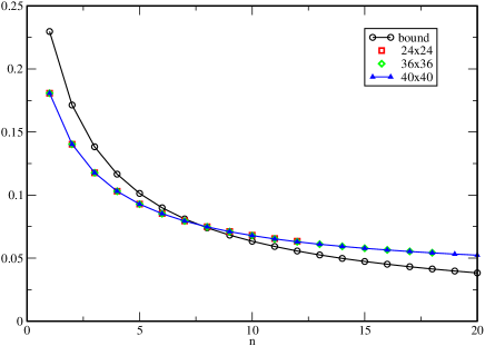
Figure 1: Bound on $\bar{g}(n)$ obtained from Eq.9 and $\bar{g}(n)$ for $24\times 24$, $36\times 36$ and $40\times 40$ at $T=0.025$.

The $\bar{g}(n)$ as defined in Eq.9 were calculated by the Quantum Monte Carlo method BW . The results, displayed in table 1, show that the $\bar{g}(n)$ calculated by Quantum Monte Carlo cross the bound obtained by integrating over $f_{q}$ at $n=8$. This is also depicted in Fig. 1. Thus inequality Eq.Néel order in the two-dimensional $S=\frac{1}{2}$-Heisenberg Model is violated and Néel order must exists in the two-dimensional antiferromagnetic Heisenberg model with $S=\frac{1}{2}$ at $T=0$.

n	Bound	$T=0.005$	$T=0.025$	$T=0.075$
1	2.297e-01	1.80799e-01 $\pm$ 3.63e-06	1.80794e-01	1.80792e-01
2	1.714e-01	1.40308e-01 $\pm$ 5.63e-06	1.40302e-01	1.40298e-01
3	1.383e-01	1.17686e-01 $\pm$ 6.84e-06	1.17678e-01	1.17670e-01
4	1.166e-01	1.03005e-01 $\pm$ 7.67e-06	1.02997e-01	1.02985e-01
5	1.013e-01	9.27815e-02 $\pm$ 8.27e-06	9.27743e-02	9.27544e-02
6	8.990e-02	8.52115e-02 $\pm$ 8.73e-06	8.52048e-02	8.51770e-02
7	8.107e-02	7.93875e-02 $\pm$ 9.10e-06	7.93811e-02	7.93436e-02
8	7.400e-02	7.47551e-02 $\pm$ 9.40e-06	7.47496e-02	7.47012e-02
9	6.820e-02	7.09844e-02 $\pm$ 9.64e-06	7.09795e-02	7.09191e-02
10	6.334e-02	6.78504e-02 $\pm$ 9.85e-06	6.78464e-02	6.77734e-02
11	5.921e-02	6.52055e-02 $\pm$ 1.00e-05	6.52021e-02	6.51163e-02
12	5.563e-02	6.29418e-02 $\pm$ 1.02e-05	6.29389e-02	6.28404e-02
13	5.252e-02	6.09835e-02 $\pm$ 1.03e-05	6.09806e-02	6.08695e-02
14	4.976e-02	5.92718e-02 $\pm$ 1.04e-05	5.92692e-02	5.91456e-02
15	4.732e-02	5.77638e-02 $\pm$ 1.06e-05	5.77617e-02	5.76255e-02

Table 1: Bound obtained by integrating numerically over the right hand side of Eq.Néel order in the two-dimensional $S=\frac{1}{2}$-Heisenberg Model compared with $\bar{g}(n)$ for a $40\times 40$ lattice and different temperatures.

There are three type of corrections to the data of table 1, which need to be taken into account, but which, as we shall show in the following, do not change the above conclusion of a crossing of the curves at $n=8$:

(i) effects of finite temperature,

(ii) effects of the finiteness of the system,

(iii) statistical errors.

In the following we comment on how these corrections modify the data.

(i) The Quantum Monte Carlo data presented are at $T\geq 0.005$. The overall effect of finite temperature is to lower the absolute value of the correlations and therefore also the value of the $\bar{g}(n)$. The effect of finite temperature is to shift the crossing of the bound and $\bar{g}(n)$ to larger n, or eventually to destroy a crossing completely.

The functional dependence of the internal energy $U(T)$, which up to an overall factor $3z$ ($z=2$ is the coordination number of the two-dimensional square lattice) equals the correlation-function at distance one, has been determined for low $T$ by spin wave theory Kubo ; Oguchi as

$$U(T)=-e_{0}+bT^{3}.$$ (11)

The coefficient is given in Taka as $b=\frac{\zeta(3)}{2e_{0}\pi}\approx 0.2853626$, so the correction for distance one is $\approx\frac{b}{6}10^{-7}$, which is two orders of magnitude smaller than the statistical error, (see point (iii)).

For distances larger than one, we fitted the data as a function of temperature (taking the exponent of T as fit parameter) for $T=0.005,0.025,0.05,0.075$ and found the corrections due to finite temperature all of the order of $10^{-5}$, which is the order of the statistical error. Therefore we do not give any finite temperature corrections.

(ii) The absolute value of the correlations in the thermodynamic limit are smaller than in systems of finite size. This means that the effect of finite system size is opposite to the effect of temperature. The finite size behaviour of the ground state energy is well studied for the Heisenberg model on the square lattice. Arguments originating from the quantum nonlinear sigma model description CHN of the Heisenberg model to lowest order in system size give

$$-e_{0}=-e_{0}(N)+\frac{c}{N^{3}},\ \ \text{with}\ \ c>0$$ (12)

where $-e_{0}(N)$ is the ground state energy of a system of size $N\times N$. Though the corrections are not substantial, they do effect the results, and taking into account, that the finite size errors in contrast to the finite temperature effects, might falsely lead to a crossing, we extrapolated the data for $N=24...40$ using the functional dependence Eq.12, which we found well satisfied also for larger distances. The results are shown in table 2. One sees that the numeric values are changed but the crossing point is still at $n=8$.

n	Bound	$T=0.025$	T=0.025 extrapolated
1	2.297e-01	1.80794e-01	1.80791e-01 $\pm$ 5.09e-06
2	1.714e-01	1.40302e-01	1.40295e-01 $\pm$ 7.87e-06
3	1.383e-01	1.17678e-01	1.17668e-01 $\pm$ 9.53e-06
4	1.166e-01	1.02997e-01	1.02983e-01 $\pm$ 1.07e-05
5	1.013e-01	9.27743e-02	9.27534e-02 $\pm$ 1.15e-05
6	8.990e-02	8.52048e-02	8.51762e-02 $\pm$ 1.21e-05
7	8.107e-02	7.93811e-02	7.93428e-02 $\pm$ 1.26e-05
8	7.400e-02	7.47496e-02	7.46995e-02 $\pm$ 1.30e-05
9	6.820e-02	7.09795e-02	7.09154e-02 $\pm$ 1.34e-05
10	6.334e-02	6.78464e-02	6.77663e-02 $\pm$ 1.37e-05
11	5.921e-02	6.52021e-02	6.51035e-02 $\pm$ 1.39e-05
12	5.563e-02	6.29389e-02	6.28188e-02 $\pm$ 1.41e-05
13	5.252e-02	6.09806e-02	6.08346e-02 $\pm$ 1.43e-05
14	4.976e-02	5.92692e-02	5.90923e-02 $\pm$ 1.45e-05
15	4.732e-02	5.77617e-02	5.75473e-02 $\pm$ 1.46e-05

Table 2: Bound obtained by integrating numerically over the right hand side of Eq.Néel order in the two-dimensional $S=\frac{1}{2}$-Heisenberg Model compared with $\bar{g}(n)$ extrapolated for N=40,36,32,24 at $T=0.025$.

(iii) We compute $\Delta x=\frac{1}{\sqrt{N_{MC}}}\sqrt{\langle x^{2}\rangle-\langle x\rangle^{2}}$ (where the observable x stands for the value of a correlation at a given distance, temperature and system size and $N_{MC}$ is the number of Monte Carlo iterations), which is a reliable estimate for the statistical error of the mean value $\langle x\rangle$, since for the algorithm of Ref.BW the autocorrelation time is of order one and the Monte Carlo configurations are almost independent. To assess the quality of our error analysis we also returned to the case of the one-dimensional antiferromagnetic Heisenberg model ( see Appendix ) and compared results with independent streams of random numbers.

To calculate an upper limit to the errors of $\bar{g}(n)$, the errors of the correlations where added up ( being evaluated with the same configurations, they are not independent).

To conclude, the error analysis shows that the short range correlations entering Eq.9 were determined with sufficiently high accuracy to prove the existence of a crossing of the bound and the Quantum Monte Carlo data for $\bar{g}(n)$ at $n=8$ and therefore to show the existence of long range order.

Appendix

(1) In this Appendix we list the correlations of a one-dimensional Heisenberg model with periodic boundary conditions and chain length $N=400$ at T=0.005 compared with results of Ref.SST for infinite chain length and $T=0$.

Distance	Quantum Monte Carlo	Bethe-Ansatz
0	0.25000000 ( 0)
1	-0.14771586 (198)	-0.1477157268
2	0.06067787 (324)	0.0606797699
3	-0.05024194 (282)	-0.0502486272
4	0.03464515 (281)	0.0346527769
5	-0.03088096 (260)	-0.0308903666
6	0.02443619 (255)	0.0244467383
7	-0.02248413 (242)	-0.0224982227
8	0.01895736 (236)

Table 3: Correlations for a chain with $N=400$ sites at T/J=0.005 compared with results from Ref. SST .

For the internal energy $U(T)$ of the Heisenberg chain the temperature dependence for low $T$ is $U(T)=-e_{0}^{1}+aT^{2}$ with the ground-state energy $e_{0}^{1}=0.4431471804$ for 400 sites and $e_{0}^{1}=-\frac{1}{4}+\ln 2$ for the infinite size systemHulthen . and the coefficient $a=\frac{1}{3}$ given in Ref. Babujian ; Affleck . This means that the correction for the correlations in table3 due to finite temperatures are of the order of $10^{-5}$.

(2) The exact values of the correlation functions DGHK ; Dam for distance one and two at $T=0$ for a chain with 400 sites are $\langle S^{3}_{0}S^{3}_{1}\rangle_{400}=-0.147717441765735$ and $\langle S^{3}_{0}S^{3}_{2}\rangle_{400}=0.0606813790491800$. The above data show that the error analysis concerning statistical errors and finite temperature effects is consistent.

Acknowledgement

I am indebted to Prof. E.H. Lieb for bringing the problem of longrange order to my attention and for his interest in this work.

References

- (1) F.J. Dyson, E.H. Lieb and B. Simon, J.Stat.Phys. 18 335-383 (1978).
- (2) T. Kennedy, E. H.Lieb and S. Shastry, J.Stat.Phys. 53, 1019-1030,(1988).
- (3) I. Affleck, T. Kennedy, E.H. Lieb and H. Tasaki, Comm. Math. Phys. 115:477-528.
- (4) E. Jordão Neves and J. Fernando Perez, Phys.Lett.114A 331-333 (1986).
- (5) M. Gross, E. Sanchez-Velasco, and E. Siggia, Phys.Rev.B 39 2484(1989).
- (6) M. Suzuki, Commun. Math. Phys. 51, (1976).
- (7) H.G. Evertz, G. Lana, M.Marcu, Phys. Rev. Lett 70, 875 (1993).
- (8) E. Farhi and S. Gutmann, Ann.Phys. (N.Y.)213, 182 (1992).
- (9) B. B. Beard and U. -J. Wiese, Phys. Rev. Lett. 77, 5130 (1996).
- (10) J. Sato, M. Shiroishi, M. Takahashi hep-th/0507290.
- (11) J.Damerau, F.Göhmann, N.P.Hasenclever, A.Klümper, cond-mat/0701463.
- (12) A. W. Sandvik, Phys.Rev.B56 (1997) 11678.
- (13) R. Kubo, Phys.Rev.87, 568 (1952).
- (14) T. Oguchi, Phys. Rev.117, 117 (1960).
- (15) M. Takahashi, Phys. Rev.B 40, 2494 (1989).
- (16) S. Chakravaty, B.I. Halperin, D.R. Nelson, Phys.Rev.B39,2344(1989).
- (17) L. Hulthén, Arkiv Mat.Astron.Fysik 26A,1 (1938).
- (18) H.M. Babujian, Nucl.Phys. B215, 317 (1982).
- (19) I. Affleck, Phys.Rev.Lett. 56,746 (1986).
- (20) J. Damerau, private communication.