Interference effects in above-threshold ionization from diatomic molecules: determining the internuclear separation

Abstract

We calculate angle-resolved above-threshold ionization spectra for diatomic molecules in linearly polarized laser fields, employing the strong-field approximation. The interference structure resulting from the individual contributions of the different scattering scenarios is discussed in detail, with respect to the dependence on the internuclear distance and molecular orientation. We show that, in general, the contributions from the processes in which the electron is freed at one center and rescatters off the other obscure the interference maxima and minima obtained from single-center processes. However, around the boundary of the energy regions for which rescattering has a classical counterpart, such processes play a negligible role and very clear interference patterns are observed. In such energy regions, one is able to infer the internuclear distance from the energy difference between adjacent interference minima.

I Introduction

The interaction of matter with an intense laser field ($I\gtrsim 10^{13}\mathrm{W/cm}^{2}$) leads to several phenomena, such as above-threshold ionization (ATI) or high-order harmonic generation (HHG). Such phenomena owe their existence to physical mechanisms, in which an electron reaches the continuum, by tunneling or multiphoton ionization, at an instant $t^{\prime}$. Subsequently, it is accelerated by the field and driven back towards its parent ion, or molecule, with which it rescatters or recombines at a later time $t$ tstep . Such laser-induced recombination or rescattering processes take place within a fraction of a laser-field cycle. The period of a typical near-infrared Ti:sapphire laser pulse is $T=2\pi/\omega\sim 2.6\mathrm{fs}$. Thus, HHG and ATI occur on a time scale of hundreds of attoseconds Scrinzi2006 . Hence, above-threshold ionization and high-order harmonic generation may be employed for probing, or even controlling, dynamic processes with attosecond and sub-angstrom resolution.

This fact, together with new alignment techniques, has opened a whole new range of possibilities for studying molecules in strong laser fields, employing high-energy photoelectrons or high-order harmonic radiation. Concrete examples are the attosecond reconstruction of the nuclear motion in a molecule Baker2006 , the real-time imaging of vibrational wavepackets vibration , the tomographic reconstruction of molecular orbitals Itatani2004 , the time-resolved measurement of intramolecular quantum-interference effects tokyo2005 , or the determination of internuclear distances Hu2005 .

These applications are a direct consequence of the fact that a molecule possesses a very specific configuration of ions from which the electron may leave, or off which it may rescatter causing above-threshold ionization, or recombine generating high-harmonics. This leads to characteristic quantum-interference patterns in the HHG or ATI spectra, in which structural information about the molecule is hidden. This is true both for polyatomic organic and diatomic molecules interfexp ; tokyo2005 ; Hu2005 ; MBBF00 ; doubleslit ; KBK98 ; ATIangleexp ; Madsen ; Usach2006 ; Usachenko ; Kansas ; Hetzheim2005 ; PRACL2006 ; DM2006 ; SFAvibrMads ; SFAvibrLein ; SFAvibrBeck ; fewcyc ; elliptical . In particular for diatomic molecules, it has been shown that the high-order harmonic or ATI spectra exhibit overall maxima and minima, which are highly dependent on the spatial separation between both centers in the molecules, and can be described as the interference between two radiating point sources. In this sense, HHG or ATI by a diatomic molecule may be viewed as the microscopic analog of a double-slit experiment tokyo2005 ; MBBF00 ; doubleslit . Furthermore, such features depend on the symmetry of the highest occupied molecular orbitals, and on the alignment angle of the molecule with respect to the laser-field polarization tokyo2005 ; Hu2005 ; MBBF00 ; doubleslit ; KB2005 ; KBK98 ; Madsen ; Usach2006 ; Usachenko ; Kansas ; Hetzheim2005 ; PRACL2006 ; DM2006 ; SFAvibrMads ; SFAvibrLein ; SFAvibrBeck .

Specifically in the diatomic case, several aspects of this interference have been extensively studied in the past few years, such as the influence of the orbital symmetry, the internuclear distance, the alignment angles tokyo2005 ; Hu2005 ; MBBF00 ; doubleslit ; KB2005 ; KBK98 ; Madsen ; Usach2006 ; Usachenko ; Kansas ; Hetzheim2005 ; PRACL2006 ; DM2006 , and molecular vibration SFAvibrMads ; SFAvibrLein ; SFAvibrBeck , as well as the role of the laser-field shape fewcyc ; fewcycvibr or polarization elliptical . Furthermore, an adequate modeling of bound molecular states, in comparison with existing ionization experiments ATIangleexp , has also raised considerable debate Usachenko ; Usach2006 ; Madsen ; DM2006 .

For that purpose, both the purely numerical solution of the time-dependent Schrödinger equation Hu2005 ; doubleslit ; KB2005 , and the strong-field approximation KBK98 ; MBBF00 ; Madsen ; Usach2006 ; Usachenko ; Kansas ; PRACL2006 ; DM2006 ; SFAvibrMads ; SFAvibrLein ; SFAvibrBeck have been employed. The latter method allows a transparent physical interpretation of the phenomena in question as laser-induced rescattering or recombination processes, and permits a clear space-time picture, which can be related to the classical orbits of an electron in a strong laser field orbitshhg . For a diatomic molecule, there exist two main rescattering or recombination scenarios: the electron born through ionization at the center $C_{i}$ upon its return may recollide and interact with either the same ion $(C_{i})$, or with the other one ( $C_{j}$ $(i\neq j)$) Such processes have been taken into account for high-order harmonic generation employing a two-center zero-range potential KBK98 ; Hetzheim2005 , using Bessel function expansions Usach2006 , and by means of saddle-point methods Hetzheim2005 ; PRACL2006 .

In this paper, we calculate the energy spectra and angular distributions of ATI produced electrons in linearly polarized laser fields, within the framework of the strong-field approximation (SFA) and the single-active electron approximation (SAE). We employ a zero-range potential model similar to that in KBK98 , and consider both the direct electrons, which reach the detector without interacting with their parent molecule, and the electrons that suffer a single act of rescattering before reaching the detector. In the latter case, we put particular emphasis on interference effects: A final state with given momentum outside the laser field can be reached via two different scenarios. An electron can be born at and rescatter off the same center, or it can be born at one center and rescatter off the other. We show that the processes involving two centers, in general, obscure the interference patterns in the ATI spectra, in almost all energy-angle regions. An exception, however, is the boundary of the region that after tunneling is classically accessible to the ionized electron, in other words, the region before the classical cutoff. Near this boundary, the two-center processes yield negligible contributions, and one may identify very clear interference patterns. This makes it possible to provide a recipe to determine the internuclear distance $R$ out of the angle-resolved ATI spectra. Throughout the article we will use the velocity gauge and atomic units $(e=m=\hbar=1,\ c=137)$.

The paper is organized as follows: In Sec. II we provide the ATI transition amplitudes for the direct and for the rescattered electrons, which in Sec. III are employed to compute the ATI spectra. The interference patterns in the spectra are analyzed with respect to molecular orientation, internuclear distance, and the position of the detector with respect to the polarization of the laser field and the molecular axis (Sec III.1). In Sec. III.2, we present angle-resolved spectra, from which we infer the internuclear distance. Finally, in Sec. IV, we summarize the paper.

II Transition amplitudes

The transition amplitude for direct ionization, within the strong-field approximation (SFA) footnote , is given by the Keldysh-Faisal-Reiss amplitude KelFaisReiss

$$M_{\mathbf{p}}=-i\int_{-\infty}^{\infty}dt\langle\Psi_{\mathbf{p}}^{(V)}(t)|V|\Psi_{0}(t)\rangle,$$ (1)

where $|\Psi_{0}(t)\rangle=|\Psi_{0}\rangle\exp(i|E_{0}|t)$. The amplitude describes an electron, initially in the ground state $|\Psi_{0}\rangle$, that is injected in the continuum by the laser field overcoming the ionization potential $|E_{0}|$, and reaches the detector with final momentum $\mathbf{p}$. The form of the transition amplitude given here, which contains the binding potential $V(\mathrm{r})$ rather than the interaction with the laser field, was first presented in Ref. PPT . In the SFA, the final state with momentum $\mathbf{p}$ is described by a Volkov state, which in velocity gauge has the form

$$\langle\mathbf{r}|\Psi_{\mathbf{p}}^{(V)}(t)\rangle=\frac{1}{(2\pi)^{3/2}}e^{i\mathbf{p}\cdot\mathbf{r}}e^{-\frac{i}{2}\int_{-\infty}^{t}d\tau[\mathbf{p}+\mathbf{A}(\tau)]^{2}}.$$ (2)

In the amplitude (1), the electron once ionized does not interact with the ion (that is, with the binding potential $V$) anymore. If we allow for at most one single act of rescattering, the amplitude (1) is replaced by

$$M_{\mathbf{p}}^{(0,1)} = -\int_{-\infty}^{\infty}dt\int_{-\infty}^{t}dt^{\prime}$$ (3)

$$\times\langle\Psi_{p}^{(V)}(t)|VU^{(V)}(t,t^{\prime})V|\Psi_{0}(t^{\prime})\rangle.$$

Here, $U^{(V)}(t,t^{\prime})$ denotes the Volkov time-evolution operator, which describes the evolution of the electron in the presence of the external laser field, ignoring the binding potential. Equation (3) incorporates direct ionization, as described by Eq. (1), as well as ionization followed by rescattering (for details, see, e.g., Ref. LKKB97 ).

In order to apply Eqs. (1) and (3) to a diatomic molecule, we consider the two-center binding potential

$$V(\mathbf{r})=V_{0}(\mathbf{r}-\mathbf{R}_{1})+V_{0}(\mathbf{r}-\mathbf{R}_{2}),$$ (4)

where $\mathbf{R}_{i}\ (i=1,2)$ denote the coordinates of the centers $C_{i}\ (i=1,2).$ For the ground-state wave function, we employ a linear combination of atomic orbitals (LCAO):

$$\Psi(\mathbf{r})=c_{1}\Psi_{0}(\mathbf{r}-\mathbf{R}_{1})+c_{2}\Psi_{0}(\mathbf{r}-\mathbf{R}_{2}).$$ (5)

Specifically, we will use the zero-range potential

$$V(\mathbf{r})=\frac{2\pi}{\kappa}\delta(\mathbf{r})\frac{\partial}{\partial r}r,$$ (6)

whose single bound state is described by the wave function

$$\Psi_{0}(\mathbf{r})=\left(\frac{\kappa}{2\pi}\right)^{1/2}\frac{1}{r}e^{-\kappa r},$$ (7)

with $\kappa=\sqrt{2|E_{0}|}$. The regularization operator $\partial/\partial r\;r$ acts on the wave function to its right in order to satisfy the proper boundary conditions at the origin Fermi1936 . For direct ionization by a monochromatic linearly polarized laser field

$$\mathbf{A}(t)=A_{0}\cos\omega t\;\mathbf{e},$$ (8)

the evaluation of the amplitude (1) is straightforward. Taking $\mathbf{R}_{1}=\mathbf{R}/2$ and $\mathbf{R}_{2}=-\mathbf{R}/2$, so that $\mathbf{R}$ is the internuclear distance of the two centers, one obtains by expanding the exponent in the Volkov wave function in Eq. (2) into Bessel functions

$$M_{\mathbf{p}}^{0} = \frac{2F}{(2\pi)^{\frac{3}{2}}}\cos\left(\frac{\mathbf{p}\cdot\mathbf{R}}{2}\right)\sum_{N,l}\delta\left(\frac{p^{2}}{2}+U_{p}+\left|E_{0}\right|-N\omega\right)$$ (9)

$$\times J_{l}\left(\frac{U_{p}}{2\omega}\right)J_{-(2l+N)}\left(\frac{2\mathbf{p\cdot e}}{\omega}\sqrt{U_{p}}\right),$$

where $U_{p}=A_{0}^{2}/4$ denotes the ponderomotive energy of the laser field (8). The prefactor, which is proportional to

$$F=-\kappa+\exp(-\kappa R)/R,$$ (10)

is of no relevance, since we do not attempt to calculate total ionization rates. It is, however, worth mentioning that the limit of $R\rightarrow 0$ is not straightforward. Below we will not face this limit. For a more detailed discussion, see, e.g., Refs. KMJ91 ; KBK98 .

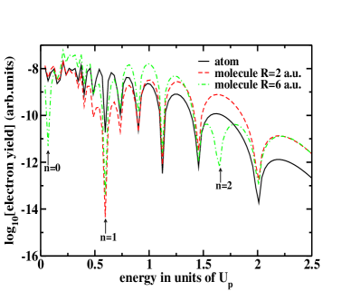
Figure 1: (Color online) ATI spectra of the direct electrons in the laser polarization direction in the atomic and molecular case, for a molecule aligned parallel to a laser field of frequency $\omega=0.058$ a.u. and ponderomotive potential $U_{p}=2.08$ a.u. We consider a symmetric combination of atomic orbitals [$c_{1}=c_{2}=1/\sqrt{2}$ in Eq. (5)], with ionization potential $|E_{0}|=0.9$ a.u. In order to facilitate the comparison, the same ionization potential $V_{0}(\mathbf{r})$ was chosen in the atomic and molecular cases. The arrows mark the various destructive interference energies $(n=0,1,2)$ for $R=6$ a.u..

The only difference between the matrix element (9) for a molecule and the corresponding matrix element for an atom, besides the $R$-dependent prefactor, is the presence of the term $\cos(\mathbf{p\cdot R}/2)$. This term describes the interference of electron orbits with momentum $\mathbf{p}$ originating from one or the other center of the two-center potential (4). The cosine term comes from assuming a symmetric combination of orbitals in the ground-state wave function (5), so that $c_{1}=c_{2}=1/\sqrt{2}$. For an antisymmetric combination, so that $c_{1}=-c_{2}$, the cosine is replaced by a sine, leading to suppression of electrons with low momenta due to destructive interference MBBF00 ; interfexp ; doubleslit . The interference factor $\cos(\mathbf{p\cdot R}/2)=\cos(pR\cos\theta/2)$ yields destructive interference for electrons with energies

$$E\equiv\frac{p^{2}}{2}=\frac{1}{2}\left(\frac{(2n+1)\pi}{R\cos\theta}\right)^{2}$$ (11)

for integer $n$. An illustration of the interference effect is given in Fig. 1, which shows the spectrum of the direct electrons for an atom and for a symmetric diatomic molecule aligned parallel to the laser-field polarization. The clearly visible sharp dips in the spectrum, due to destructive interference, are indicated by the arrows in the figure. Next, we turn to the evaluation of the matrix element (3), which allows rescattering. With the two-center potential (4) and the symmetric ground-state wave function (5), the matrix element reads

$$M_{\mathbf{p}} = \frac{-i}{(2\pi)^{3/2}}\int_{-\infty}^{\infty}dt\int_{-\infty}^{t}dt^{\prime}\int d^{3}r\int d^{3}r^{\prime}\;e^{-i\mathbf{p}\cdot\mathbf{r}}e^{\frac{i}{2}\int_{-\infty}^{t}d\tau(\mathbf{p}+\mathbf{A}(\tau))^{2}}\left[V_{0}(\mathbf{r}+\mathbf{R/2})+V_{0}(\mathbf{r}-\mathbf{R/2})\right]$$ (12)

$$\times U^{(V)}(\mathbf{r}t;\mathbf{r^{\prime}}t^{\prime})\left[V_{0}(\mathbf{r^{\prime}}+\mathbf{R/2})+V_{0}(\mathbf{r^{\prime}}-\mathbf{R/2})\right]\left[\Psi_{0}(\mathbf{r^{\prime}}+\mathbf{R/2})+\Psi_{0}(\mathbf{r^{\prime}}-\mathbf{R/2})\right]e^{i|E_{0}|t^{\prime}}\;.$$

For the zero-range potential (6), the integrations over space can be carried out easily LKKB97 , which leaves a two-dimensional integral over the ionization time $t^{\prime}$ and the rescattering time $t$. For finite-range potentials, one may proceed by introducing form factors and employing saddle-point methods. In this case, the single-center prefactors cause an overall decrease of the yield for increasing photoelectron energy. There are, however, no significant changes in the interference patterns in comparison with the zero-range case, since these prefactors do not influence the action or the cosine factor. For a detailed discussion of the single-atom case, see, e.g., Ref. Faria2002 .

We split the eight integrals into those where the electron rescatters off the same center from which it was ionized $(\mathbf{r}=\mathbf{r^{\prime}}=\pm\mathbf{R/2})$ and those where it rescatters off the opposite center $(\mathbf{r}=-\mathbf{r^{\prime}}=\pm\mathbf{R/2})$. We refer to the respective terms by $M^{ij}$ where $i=+,-$ denote the center of ionization and $j=+,-$ the center of rescattering. The integrals $M^{++}$ and $M^{--}$, which specify the electrons coming from and rescattering off the same center, are essentially identical to the corresponding results for an atom LKKB97 . The structure of the molecule is reflected in the integrals $M^{+-}$ and $M^{-+}$, which characterize the electrons that experience the presence of both centers. Evaluating the remaining two integrals over $t$ and $t^{\prime}$, we substitute $t^{\prime}=t-\tau$. The doubly infinite integral over $t$ then yields a $\delta$-function expressing energy conservation, while the semi-infinite integration over $\tau$ has to be calculated numerically. Expanding all oscillating exponents in terms of Bessel functions, we obtain for the transition amplitudes

$$M_{\mathbf{p}}^{++}+M_{\mathbf{p}}^{--} = 2F\cos\left(\frac{\mathbf{p\cdot R}}{2}\right)\sum_{N}\delta\left(\frac{p^{2}}{2}+U_{p}+|E_{0}|-N\omega\right)\sum_{l=-\infty}^{\infty}J_{-(2l+N)}\left(\frac{2\mathbf{p\cdot e}}{\omega}\sqrt{U_{p}}\right)$$ (13)

$$\times\int_{0}^{\infty}d\tau\left(\frac{i}{2\pi\tau}\right)^{3/2}\left\{e^{-i(|E_{0}|\tau+l\alpha)}e^{-iU_{p}\tau[1-(\frac{\sin\omega\tau/2}{\omega\tau/2})^{2}]}J_{l}\left(\frac{U_{p}}{2\omega}A\right)-J_{l}\left(\frac{U_{p}}{2\omega}\right)\right\}$$

$$= 2F\cos\left(\frac{\mathbf{p\cdot R}}{2}\right)M_{\mathbf{p}}^{(\mathrm{atom})},$$

$$M_{\mathbf{p}}^{+-} = Fe^{-i\frac{\mathbf{p\cdot R}}{2}}\sum_{N,l}\delta\left(\frac{p^{2}}{2}+U_{p}+|E_{0}|-N\omega\right)\int_{0}^{\infty}d\tau\left(\frac{i}{2\pi\tau}\right)^{3/2}$$ (14)

$$\times\left\{e^{i\frac{R^{2}}{2\tau}}e^{-i[|E_{0}|\tau+l\alpha+(2l+N)\beta_{-}]}e^{-iU_{p}\tau[1-(\frac{\sin\omega\tau/2}{\omega\tau/2})^{2}]}J_{l}\left(A\frac{U_{p}}{2\omega}\right)J_{-(2l+N)}\left(\frac{2\sqrt{U_{p}}}{\omega}B_{-}\right)\right\},$$

$$M_{\mathbf{p}}^{-+} = Fe^{i\frac{\mathbf{p\cdot R}}{2}}\sum_{N,l}\delta\left(\frac{p^{2}}{2}+U_{p}+|E_{0}|-N\omega\right)\int_{0}^{\infty}d\tau\left(\frac{i}{2\pi\tau}\right)^{3/2}$$ (15)

$$\times\left\{e^{i\frac{R^{2}}{2\tau}}e^{-i[|E_{0}|\tau+l\alpha+(2l+N)\beta_{+}]}e^{-iU_{p}\tau[1-(\frac{\sin\omega\tau/2}{\omega\tau/2})^{2}]}J_{l}\left(A\frac{U_{p}}{2\omega}\right)J_{-(2l+N)}\left(\frac{2\sqrt{U_{p}}}{\omega}B_{+}\right)\right\}.$$

The real quantities $A$, $B_{\pm}$ and the phases $\alpha$ and $\beta_{\pm}$ are defined by

$$Ae^{-i\alpha} = e^{-2i\omega\tau}+\frac{8i}{\omega\tau}\sin^{2}\frac{\omega\tau}{2}e^{-i\omega\tau},$$ (16)

$$B_{\pm}e^{-i\beta_{\pm}} = \mathbf{p\cdot e}\pm\frac{\mathbf{R\cdot e}}{\tau}[i\sin\omega\tau-(1-\cos\omega\tau)].$$ (17)

Upon $\mathbf{R}\rightarrow-\mathbf{R}$, we have $B_{\pm}\exp(-i\beta_{\pm})\rightarrow B_{\mp}\exp(-i\beta_{\mp})$. Consequently, the matrix element $M_{\mathbf{p}}$ does not change when $\mathbf{R}\rightarrow-\mathbf{R}$. The complete matrix element is the sum of the terms (13) – (15),

$$M_{\mathbf{p}}=M_{\mathbf{p}}^{++}+M_{\mathbf{p}}^{--}+M_{\mathbf{p}}^{+-}+M_{\mathbf{p}}^{-+}.$$ (18)

The first two terms describe electrons originating from and rescattering off the same center. They are proportional to the atomic ionization amplitude $M_{\mathbf{p}}^{(\mathrm{atom})}$ LKKB97 multiplied by the wave-function overlap $F$ and the two-center interference factor $\cos(\mathbf{p\cdot R}/2)$, which we observed for the direct electrons in Eq. (9). The behavior of the exchange terms $M_{\mathbf{p}}^{+-}$ and $M_{\mathbf{p}}^{-+}$ is more complicated and will be discussed below.

The transition amplitude $M_{\mathbf{p}}$ simplifies enormously when the molecule is aligned perpendicularly to the field so that $\mathbf{R}\cdot\mathbf{e}=0$. Equation (17) shows that in this case $B_{+}=B_{-}$ and $\beta_{+}=\beta_{-}=0$. Hence, the integrals on the right-hand side of Eqs. (14) and (15) are equal and $M_{\mathbf{p}}^{+-}+M_{\mathbf{p}}^{-+}$ becomes proportional to $2\cos(\mathbf{p}\cdot\mathbf{R}/2)$ just like $M_{\mathbf{p}}^{++}+M_{\mathbf{p}}^{--}$. If, in addition, the electron is emitted perpendicularly to the field so that also $\mathbf{p}\cdot\mathbf{e}=0$, then $B_{+}=B_{-}=0$ and we have $M_{\mathbf{p}}=0$ unless $N$ is even.

Substituting $\tau\to\tau/\omega$ in Eqs. (13)–(17) one can see that the amplitudes $M^{ij}_{\mathbf{p}}$ and their sum $M_{\mathbf{p}}$ depend on the parameters of the problem through the dimensionless quantities $p^{2}/\omega$, $U_{p}/\omega$, and $\omega R^{2}$ when the relative orientations of the vectors $\mathbf{R}$, $\mathbf{p}$, and $\mathbf{e}$ are kept fixed.

III Photoelectron spectra

In this section we discuss the ATI spectra computed employing the transition matrix elements (1) and (3), and a symmetric combination of equivalent centers [$c_{1}=c_{2}=1/\sqrt{2}$ in Eq. (5)]. For the sake of simplicity, in the comparison between the atomic and molecular case the same ionization potential $V_{0}$ is chosen. Specifically, we take $|E_{0}|=0.9$ a.u. in Eqs. (5) and (7) throughout footnIp . In Sec. III.1, we perform a detailed analysis of the interference patterns with respect to the molecular orientation, rescattering scenarios, and the direction of electron emission, while in Sec. III.2 we provide a recipe for measuring the internuclear distance from an analysis of the interference patterns in the angle-resolved spectra.

III.1 Analysis of the interference patterns

As a first step, we investigate how the interference patterns are influenced by the orientation of the molecule with respect to the laser-polarization direction. Such results are displayed in Figs. 2 and 3 for parallel and perpendicular orientations, respectively. In both cases, we compare the entire ATI spectrum consisting of the direct and the rescattered electrons in the atomic and the molecular case. Unless stated otherwise (cf. Fig. 5), we consider electron emission in the laser-polarization direction.

As expected from Eq. (9), for energies smaller than $2U_{p},$ the main contributions to the yield come from the direct-ionization matrix element (9). Apart from the interference-related factor of $\cos(\mathbf{p}\cdot\mathbf{R}/2)$, the transition matrix element is identical to that obtained for a single atom (cf. Fig. 1). This factor is responsible for the sharp interference dips at the positions given by Eq. (11). In the plateau energy region, however, the spectra depend on the laser-field polarization in a more complex way, as will be discussed next. In case the molecule is aligned parallel to the laser-field polarization (Fig. 2), the plateau is strongly enhanced in the molecular case, and the structure of the spectrum is very different from the atomic case and dependent on the internuclear distance $R$. Indeed, inspection of the exchange integrals (14) and (15) does not reveal any simple dependence on the internuclear distance. Generally, for the molecular case there are more pathways into a given final state. For our case of a two-center potential, there are four pathways in place of one for the atomic case. If they add coherently, a significant enhancement can result, ideally by a factor of 16, which is roughly what is observed in Fig.  2 before the cutoff. The structure caused by the cosine factor is suppressed in the plateau region. This is caused by the contribution of the processes in which the electron is ejected from one center and rescatters off the other. Such processes correspond to the transition amplitudes $M_{p}^{-+}$ and $M_{p}^{+-}$, which do not exhibit the proportionality to the cosine that is characteristic of the the one-center scattering amplitudes $M_{p}^{++}$ and $M_{p}^{--}$. A further particular feature observed in this case is the displacement of the cut-off to higher energies with increasing internuclear distance. This can be understood by the fact that an electron that moves from one center to the other may gain more energy from the field since it may be accelerated over a longer distance before it recollides.

A strikingly different behavior is observed if the molecule is aligned perpendicular to the direction of the laser field so that $\mathbf{R}\cdot\mathbf{e}=0$. In Fig. 3 we consider the case where the electron is emitted in the direction of the laser polarization so that $\mathbf{p}\cdot\mathbf{R}=0$, too. In this case, there is a general enhancement of the ATI yield in comparison to that of a single atom by roughly a factor of two for the direct electrons and a much larger factor for the rescattered electrons. Notice that the molecular spectrum is practically independent of the internuclear distance Hetzheim2005 , since the $R$ dependence of the prefactor (10) is weak for $R\gtrsim 2$ and the exponential of $R^{2}/(2\tau)$ is small for the values of $R$ that we consider and the values of $\tau$ that give the dominant contributions to the integral. The entire ATI spectrum does not show any interference structure, since the contributions from the two centers add constructively for $\mathbf{p}\cdot\mathbf{R}=0$. In fact, the cosine term in the matrix elements $M_{\mathbf{p}}^{0}$, $M_{p}^{++}$ and $M_{p}^{--}$ simply reduces to one and the spectrum therefore looks like that of an atom. Specifically within the plateau, by symmetry the contributions from the two centers always interfere constructively. This results in a spectrum that is largely independent on the internuclear separation $R$, except that the plateau is enhanced, compared with the atomic case, by the existence of four pathways. Formally, this can be understood as discussed above at the end of Sec. II.

For arbitrary $\mathbf{p}\cdot\mathbf{R}$, if the electron is emitted perpendicular to the laser polarization so that $\mathbf{p\cdot e}=0$, then we see from Eqs. (16) and (17) that $B_{+}=B_{-}\!$, while $\beta_{-}=\beta_{+}+\pi$. The sum of the two exchange terms then goes like $\cos(\mathbf{p\cdot R}/2)$ for even $N$ and like $\sin(\mathbf{p\cdot R}/2)$ for odd $N$. This holds regardless of the orientation of the molecule. If the laser polarization is perpendicular to both the electron momentum and the internuclear axis, then $B_{+}=B_{-}=0$. This implies that $M_{\mathbf{p}}$ is nonzero only for integer $N$. Each other electron peak is missing.

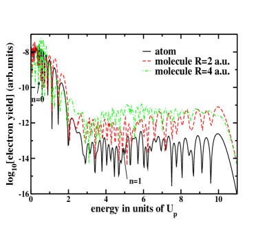
Figure 2: (Color online) Comparison of the complete ATI spectra consisting of direct and rescattered electrons in the atomic and the molecular case for internuclear distances of $R=2$ a.u. and $R=4$ a.u.. The molecule is aligned parallel to the laser-polarization direction, and the electrons are emitted in the same direction. The arrows mark the destructive interferences $(n=0,1)$ of the molecule for $R=2$ a.u.. The destructive interference for $n=1$ is already in the plateau region, where the role of exchange terms becomes important. The remaining parameters are the same as in Fig. 1.

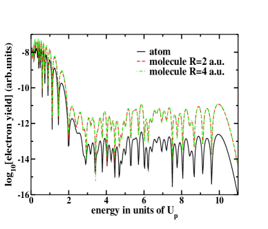
Figure 3: (Color online) The same as Fig. 2 but with the molecular axis perpendicular to the laser polarization. The electrons are emitted parallel to the laser polarization.

Next, we discuss the interference pattern in more detail by analyzing the individual contributions to the transition matrix element. In Fig. 4, we separately investigate the individual contributions to the amplitude (18). If only $M_{p}^{++}$ and $M_{p}^{--}$ are taken, a very pronounced mininum is observed near $5U_{p}.$ These matrix elements correspond to the case in which the electron is ejected from and rescatters off the same center, so that the minimum is due to the term $\cos(\mathbf{p\cdot R}/2)$. In the full spectrum $|M_{\mathbf{p}}|^{2},$ however, this minimum is absent because it is filled by the contributions from the exchange terms $M_{p}^{-+}$ and $M_{p}^{+-}$. For a given orientation of the molecule with respect to the laser field and for fixed momentum $\mathbf{p,}$ Fig. 4 shows that the contribution $|M_{p}^{-+}|^{2}$ of the scenario in which the electron is freed at the center $C_{1}$ and rescatters off at the center $C_{2}$ is different from that of $|M_{p}^{+-}|^{2}$ where it is released at $C_{2}$ and rescatters at $C_{1}$. The same has been observed for high-order harmonic generation in a two-center system KBK98 .

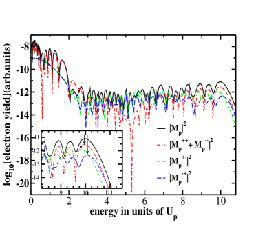
Figure 4: (Color online) Individual contributions of the various rescattering scenarios to the total amplitude (18) for a diatomic molecule with internuclear distance $R=2$ a.u. aligned parallel to the laser-field polarization, for the same molecular and field parameters as in Fig. 2. The electrons are emitted in the polarization direction. The arrows mark the respective cutoff energies for the various transition amplitude matrix elements. The inset at the lower left is an enlargement of the region near the cutoff where the direct terms and the exchange terms differ in a characteristic fashion, allowing for the determination of the internuclear separation.

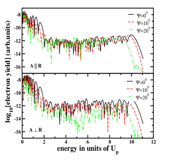
Figure 5: (Color online) Electron yield for the parameters of Fig. 1 and internuclear distance $R=2$ a.u. for different emission angles $\psi$ with respect to the polarization of the laser field. The molecule is aligned parallel (perpendicular) to the laser field in the upper (lower) panel.

The imprints of interference can still be observed if the electron is emitted away from the laser polarization direction. This will cause, however, an overall decrease in the photoelectron energies for both the direct and the rescattered electrons. Examples are presented in Fig. 5. This behavior is known from atomic ionization, and its origin is the same in the molecular case; for a discussion, see, e.g., Ref. LKKB97 .

III.2 Determining the internuclear distance

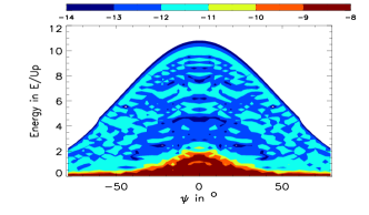
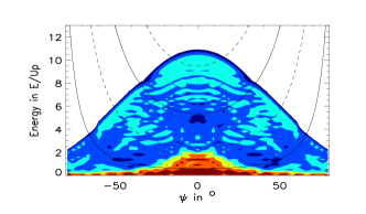
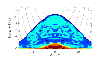
Figure 6: (Color online) Angle-resolved ATI spectra on a logarithmic scale for a diatomic molecule with internuclear distances $R=2$ a.u. and $R=3$ a.u. (middle and bottom panels, respectively), aligned parallel to the laser-field polarization, compared to the single-atom case (upper panel). The binding energy is $E_{0}=0.9$ a.u. in all cases, and the laser frequency and the ponderomotive potential are $\omega=0.058$ a.u. and $U_{p}=2.08$ a.u., respectively. The plotted lines depict the minima (solid lines) and the maxima (dashed lines) of the energy distribution given by Eq. (11).

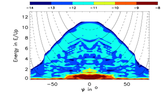
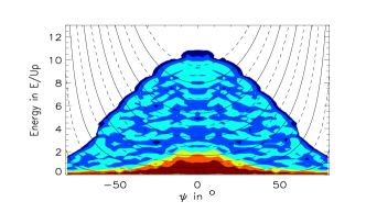
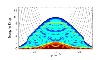
Figure 7: (Color online) Angle-resolved ATI spectra on a logarithmic scale for a diatomic molecule with ionization potential $E_{0}=0.9$ a.u. and internuclear distances $R=4$ a.u., $R=6$ a.u. and $R=8$ a.u. (upper, middle and bottom panels, respectively), aligned parallel to the laser-field polarization. The field parameters are the same as in the previous figure. The plotted lines depict the minima (solid lines) and the maxima (dashed lines) of the energy distribution given by Eq. (11).

For a complete picture of the angle-resolved ATI spectrum, not restricted to emission in particular directions, we will now present density plots. While they invariably imply loss of fine details and depend on the positioning and gradient of the false-color scale, they give a comprehensive overview of the general structure. We restrict ourselves to the case of parallel alignment . In this case the spectrum is symmetrical with respect to the internuclear axis. It is obvious that the electrons with maximal kinetic energy will be detected in the direction of the laser field.

The angle-resolved spectra displayed in Figs. 6 and 7 are very intricate and do not exhibit any simple structures. They depend strongly on the internuclear separation but do not, on a first inspection, lend themselves in any obvious way to the assignment of a specific value of $R$ to a given spectrum. Especially, owing to the presence and magnitude of the exchange terms (14) and (15), the two-center interference, which is expressed in the $\cos(\mathbf{p}\cdot\mathbf{R}/2)$ term, is not immediately visible. However, looking more closely, one can observe a very distinct manifestation of this term just near the classical boundary of the spectrum. Roughly, the latter agrees with the boundaries of the colored areas in the various panels of Figs. 6 and 7. We observe well-defined indents in the overall smooth curve that defines the classical boundary. The positions of these indents and, especially, their separations agree quite well with the interference minima predicted by Eq. (11). The figures show that the separation $\delta E$ between the indents (on the scale of $U_{p}$) monotonically decreases with increasing $R$. Hence, by comparing a measured angle-resolved spectrum with Figs. 6 and 7 we can infer the internuclear separation. For the parameters underlying Figs. 6 and 7, the resulting function $R(\delta E)$ is given in Table 1. Fig. 8 exhibits an enlargement of the relevant area around the classical cutoff for the case of $R=8$ a.u. with a higher resolution of the electron yield. The indents are very clearly visible like valleys that cut into the drop of a plateau on a topographical map.

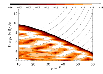
Figure 8: (Color online) Enlargement of a limited energy-angle region of Fig. 7 for $R=8$ a.u. (lowest panel) with increased resolution. The indents of Fig. 7 are distinctly visible as valleys deeply cut into the high ridge that precedes the cutoff.

An analytical formula for $R(\delta E)$ can be gained from an analytical formula for the classical cutoff energy $E(\theta)$ as a function of the angle $\theta$. Intersecting this with the energies of the interference minima given by Eq. (11) allows one to determine the function $R(\delta E)$ in dependence of the parameters of the problem. For the case of an atom, such a formula for $E(\theta)$ is actually known haso07 . At least for $R\leq 6$ a.u., Figs. 6 and 7 show that this classical boundary does not depend very strongly on the internuclear separation $R$, so that the atomic result could be employed. However, even with this simplification, the resulting formula is quite complicated and we refrain from presenting it here.

The question arises of why near the classical boundary the interference term $\cos(\mathbf{p}\cdot\mathbf{R}/2)$ roughly multiplies the angle-resolved spectrum, like it does for the direct electrons. The answer can be inferred from Fig. 4. The total ionization amplitude $M_{\mathbf{p}}$ is the superposition (13) of four different scenarios such that the electron starts from and rescatters off one or the other center. The two contributions (13) where they start from and rescatter off the same center are identical except for the geometrical phase, which leads to the cosine in Eq. (13). In contrast, the other two contributions (14) and (15) are uncorrelated since they are generated by geometrically different scenarios. Their magnitudes are different and almost nowhere do they exhibit a significant constructive interference. The two contributions (13) are individually large when the long orbit and the short orbit add constructively, as is the case specifically just before the classical cutoff. In this case, they dominate the other two terms (14) and (15) by a factor of the order of 2 to 4. Hence the complete spectrum distinctly exhibits the geometrical interference, which is expressed in the factor $\cos(\mathbf{p}\cdot\mathbf{R}/2)$.

Internuclear distances	Energy differences of the indents
of the molecule	at the spectral boundary
$R=2$ a.u.	$\delta E\approx 4.5U_{p}$
$R=3$ a.u.	$\delta E\approx 3.2U_{p}$
$R=4$ a.u.	$\delta E\approx 2.4U_{p}$
$R=6$ a.u.	$\delta E\approx 1.3U_{p}$
$R=8$ a.u.	$\delta E\approx 1.1U_{p}$

Table 1: Energy differences between adjacent indents around the classical boundary of the angle-resolved spectrum of Fig. 6. The differences are taken, for each internuclear separation, by starting with the first indent for $\Psi\geq 0^{\circ}$ as a function of the energy.

IV Conclusions

We have analyzed ATI spectra for a two-center molecule in a linearly polarized laser field. The terms of the two-center wave function contributing to the interference structure within the SFA formalism could be identified as well as the absence of the interference structure throughout most of the plateau region. We have shown that the angle-resolved spectra can be used to determine the internuclear distance of a molecule aligned with the laser field, by reading off the energy differences between subsequent interference minima at the classical boundary of the spectrum.

The validity of this method depends upon how close to reality is the angle-resolved spectrum calculated for our model molecule. Certainly, the spectrum of the direct electrons cannot be trusted for this purpose. However, high-order ATI of an atom is well described by the SFA and a zero-range potential, especially near the classical boundary LKKB97 ; for a comparison of spectra calculated from the SFA with the solution of the time-dependent Schrödinger equation, see Ref. BMB06 for the case of an atom. Experimentally, application of the method requires a high detection efficiency that allows one to obtain a sufficient number of counts down to the classical boundary.

The problem of how to extract the internuclear separation from a diffraction pattern has been addressed by a different method in Ref. Hu2005 , employing the numerical solution of the time-dependent Schrdinger equation. In Hu2005 , however, it is necessary to compute a radial distribution function from the diffraction intensity, whereas, with the method discussed in this paper, one may determine the internuclear distances directly from the spectra. The method suggested in Ref. Hu2005 has the advantage that it analyzes direct electrons and, therefore, does not require exceptionally high detection efficiency.

Finally, in a real physical system, there exist additional effects, which have not been incorporated in this model and may alter the interference patterns. Molecular vibration, for instance, causes an intensity loss in the high-harmonic signal SFAvibrLein , which may lead to a blurring in the patterns. However, recently, numerical ATI computations in which such an effect is included have shown that for H${}_{2}^{+}$ the angle-dependent interference patterns related to the double-slit physical picture remain distinguishable in the case considered fewcycvibr . Generally, the amount of blurring depends on the rigidity of the vibrational potential. Since the period of vibrations is much longer than the laser period, with a few-cycle laser pulse our method could be used to track a vibrational wave packet or the dissociation of a molecule vibration . Another feature which has not been incorporated in our model is the dependence of the ionization potential on the internuclear distance. In fact, we have taken $E_{0}$ to be constant, whereas, in reality, it decreases with $R$ KBK98 . This feature, however, will only cause an overall energy shift in the spectra. Therefore, it will not affect the distance between two consecutive minima or maxima in the patterns for constant internuclear distance (Figs. 6 and 7). Therefore, we expect our method to be applicable to real physical systems and a wide parameter range.

- (1) P. B. Corkum, Phys. Rev. Lett. 71, 1994 (1993); K. C. Kulander, K. J. Schafer, and J. L. Krause in: B. Piraux et al. eds., Proceedings of the SILAP conference, (Plenum, New York, 1993).
- (2) A. Scrinzi, M. Y. Ivanov, R. Kienberger, and D. M. Villeneuve, J. Phys. B 39, R1 (2006).
- (3) S. Baker, J. Robinson, C. Haworth, H. Teng, R. Smith, C. Chirilă, M. Lein, J. Tisch, and J. P. Marangos, Science 312, 424 (2006).
- (4) H. Niikura, F. Légaré, R. Hasbani, A. D. Bandrauk, M. Yu. Ivanov, D. M. Villeneuve, and P. B. Corkum, Nature 417, 917 (2002); H. Niikura, F. Légaré, R. Hasbani, M. Yu. Ivanov, D. M. Villeneuve, and P. B. Corkum, Nature 421, 826 (2003); E. Goll, G. Wunner, and A. Saenz, Phys. Rev. Lett. 97, 103003 (2006); F. Légaré, K. F. Lee, A. D. Bandrauk, D. M. Villeneuve, and P. B. Corkum, J. Phys. B 39, S503 (2006).
- (5) J. Itatani, J. Levesque, D. Zeidler, H. Niikura, H. Pépin, J.C. Kieffer, P. B. Corkum, and D. M. Villeneuve, Nature 432, 867 (2004).
- (6) T. Kanai, S. Minemoto, and H. Sakai, Nature 435, 470 (2005).
- (7) S. X. Hu and L. A. Collins, Phys. Rev. Lett. 94, 073004 (2005).
- (8) For experiments see, e.g., N. Hay, R. de Nalda, T. Halfmann, K. J. Mendham, M. B. Mason, M. Castillejo, and J. P. Marangos, Phys. Rev. A 62, 041803(R)(2000); C. Altucci, R. Velotta, E. Heesel, E. Springate, J. P. Marangos, C. Vozzi, E. Benedetti, F. Calegari, G. Sansone, S. Stagira, M. Nisoli, and V. Tosa, Phys. Rev. A 73, 043411 (2006); H. Ohmura, F. Ito, and M. Tachyia, Phys. Rev. A 74, 043410 (2006); and for theory T. K. Kjeldsen, C. Z. Bisgaard, L. B. Madsen, and H. Stapelfeld, Phys. Rev. A 71, 013418 (2005).
- (9) B. Shan, X. M. Tong, Z. Zhao, Z. Chang, and C. D. Lin, Phys. Rev. A 66, 061401(R) (2002); F. Grasbon, G. G. Paulus, S. L. Chin, H. Walther, J. Muth-Böhm, A. Becker, and F. H. M. Faisal, Phys. Rev. A 63, 041402(R)(2001); C. Altucci, R. Velotta, J. P. Marangos, E. Heesel, E. Springate, M. Pascolini, L. Poletto, P. Villoresi, C. Vozzi, G. Sansone, M. Anscombe, J. P. Caumes, S. Stagira, and M. Nisoli, Phys. Rev. A 71, 013409 (2005).
- (10) J. Muth-Böhm, A. Becker, and F. H. M. Faisal, Phys. Rev. Lett. 85, 2280 (2000); A. Jarón-Becker, A. Becker, and F. H. M. Faisal, Phys. Rev. A 69, 023410 (2004)
- (11) M. Lein, N. Hay, R. Velotta, J. P. Marangos, and P. L. Knight, Phys. Rev. Lett. 88, 183903 (2002); Phys. Rev. A 66, 023805 (2002); M. Lein, J. P. Marangos, and P. L. Knight, Phys. Rev. A 66, 051404(R) (2002); M. Spanner, O. Smirnova, P. B. Corkum, and M. Y. Ivanov, J. Phys. B 37, L243 (2004).
- (12) D. A. Telnov and Shih-I Chu, Phys. Rev. A 71, 013408 (2005); G. Lagmago Kamta and A. D. Bandrauk, Phys. Rev. A 71, 053407 (2005).
- (13) R. Kopold, W. Becker, and M. Kleber, Phys. Rev. A 58, 4022 (1998).
- (14) C. Guo, M. Li, J. P. Nibarger, and G. N. Gibson, Phys. Rev. A 58, R4271 (1998); M. J. DeWitt, E. Wells, and R. R. Jones, Phys. Rev. Lett. 87, 153001 (2001); E. Wells, M. J. DeWitt, and R. R. Jones, Phys. Rev. A 66, 013409 (2002); I. V. Litvinyuk, K.F. Lee, P.W. Dooley, D.M. Rayner, D.M. Villeneuve, and P.B. Corkum, Phys. Rev. Lett. 90, 233003 (2003).
- (15) T. K. Kjeldsen and L. B. Madsen, J. Phys. B 37, 2033 (2004); Phys. Rev. A 73, 047401 (2006).
- (16) C. P. J. Martiny, and L. B. Madsen, Phys. Rev. Lett. 97, 093001 (2006); ibid. 97, 169903 (2006); S. Baier, C. Ruiz, L. Plaja, and A. Becker, Phys. Rev. A 74, 033405 (2006).
- (17) S. Seltsø, J. F. McCann, M. Førre, J. P. Hansen, and L. B. Madsen, Phys. Rev. A 73, 033407 (2006).
- (18) M. Lein, P. P. Corso, J. P. Marangos, and P. L. Knight, Phys. Rev. A 67, 023819 (2003).
- (19) V. I. Usachenko, P. E. Pyak, and S.-I Chu, Laser Phys. 16, 1326 (2006).
- (20) V. I. Usachenko, and S.-I Chu, Phys. Rev. A 71, 063410 (2005); V. I. Usachenko, Phys. Rev. A 73, 047402 (2006).
- (21) H. Hetzheim, M. Sc. thesis (Humboldt Universität zu Berlin, 2005).
- (22) C. C. Chirilă and M. Lein, Phys. Rev. A 73, 023410 (2006); ibid. 74, 051401(R) (2006).
- (23) X. Zhou, X. M. Tong, Z. X. Zhao, and C. D. Lin, Phys. Rev. A 71, 061801(R) (2005); ibid. 72, 033412 (2005).
- (24) T. K. Kjeldsen and L. B. Madsen, Phys. Rev. A 71, 023411 (2005); Phys. Rev. Lett. 95, 073004 (2005); C. B. Madsen and L. B. Madsen, Phys. Rev. A 74, 023406 (2006).
- (25) M. Lein, Phys. Rev. Lett. 94, 053004 (2005); C. C. Chirilă and M. Lein, J. Phys. B 39, S437 (2006).
- (26) A. Requate, A. Becker, and F. H. M. Faisal, Phys. Rev. A 73, 033406 (2006).
- (27) D. B. Milošević, Phys. Rev. A 74, 063404 (2006).
- (28) P. Salières, B. Carré, L. LeDéroff, F. Grasbon, G. G. Paulus, H. Walther, R. Kopold, W. Becker, D. B. Milošević, A. Sanpera, and M. Lewenstein, Science 292, 902 (2001).
- (29) The SFA consists in neglecting the atomic binding potentials when the electron is in the continuum, the external laser field when the electron is bound, and the internal structure of the molecule.
- (30) L. V. Keldysh, Sov. Phys. JETP 20, 1307 (1964); F. H. M. Faisal, J. Phys. B 6, L89 (1973); H. R. Reiss, Phys. Rev. A 22, 1786 (1980).
- (31) A. Perelomov, V. Popov, and M. Terent’ev, JETP 23, 924 (1966).
- (32) A. Lohr, M. Kleber, R. Kopold, and W. Becker, Phys. Rev. A 55, R4003 (1997).
- (33) W. Becker, S. Long, and J. K. McIver Phys. Rev. A 50, 1540 (1994); M. Lewenstein, Ph. Balcou, M. Yu. Ivanov, A. L’Huillier, and P. B. Corkum Phys. Rev. A 49, 2117 (1994); W. Becker, A. Lohr, M. Kleber, and M. Lewenstein, Phys. Rev. A 56, 645 (1997).
- (34) E. Fermi, Ric. Sci. 7, 13 (1936).
- (35) P. Krstić, D. B. Milošević, and R. Janev, Phys. Rev. A 44, 3089 (1991).
- (36) C. Figueira de Morisson Faria, H. Schomerus, and W. Becker, Phys. Rev. A 66, 043413 (2002).
- (37) In reality, the ionization potential of a molecule decreases with increasing internuclear distance. This effect, however, will only cause an overall shift in the interference patterns. Since it will neither modify their shapes, nor the energy difference between neighboring maxima, it is not relevant to the present discussion. For the specific computation of this shift within the context of a zero-range model potential see, e.g., Ref. KBK98 .
- (38) W. Becker, F. Grasbon, R. Kopold, D. B. Milošević, G. G. Paulus, and H. Walther, Adv. At. Mol. Opt. Phys. 48, 36 (2002).
- (39) E. Hasović, M. Busuladžić, A. Gasibegović-Busuladžić, D. B. Milošević, and W. Becker, Laser Phys. 17, 376 (2007).
- (40) D. Bauer, D. B. Milošević, and W. Becker, J. Mod. Opt. 53, 135 (2006).