Modeling the field of laser welding melt pool by RBFNN

Abstract

Efficient control of a laser welding process requires the reliable prediction of process behavior. A statistical method of field modeling, based on normalized RBFNN, can be successfully used to predict the spatiotemporal dynamics of surface optical activity in the laser welding process. In this article we demonstrate how to optimize RBFNN to maximize prediction quality. Special attention is paid to the structure of sample vectors, which represent the bridge between the field distributions in the past and future.

I Introduction

Laser systems are efficiently applied in welding processes [1], where a laser beam is used to melt material. To maintain high performance in a welding process, efficient control should be established.

The crucial task in planning the control system is to determine representative variables which can effectively describe the welding process. For this purpose, the intensity and spatial distribution of reflected light, surface temperature values or properties of the emitted electron plasma are usually chosen. However, characteristic dynamic properties in space and time can also be obtained by recording surface optical activity in the heated zone, known as the melt pool [2].

After choosing the representative variables, extraction of evolution laws from temporal data becomes a crucial problem. To date, this problem has been extensively studied in relation to chaotic time series prediction [3, 4, 5, 6, 7]. The basis of these methods is to reconstruct a state-space from a recorded scalar time series by using an embedded technique, and then to estimate deterministic dynamic evolution from the reconstructed trajectory using statistical average estimators. We present a generalization of this approach, where the modeling of dynamic laws is extended from one dimension (time) to multiple dimensions in spatiotemporal space. This generalization requires a new embedding method, which makes feasible a reconstruction of trajectory in the state-space from spatiotemporal data. The embedded technique, which was initially developed for time series analysis, can be simply generalized to spatially related data [8, 9, 10, 11, 12] and results in a good agreement between predicted and original chaotic fields over short time scales. Since, in a properly reconstructed state-space, the modeled dynamics must have similar statistical properties to the actual dynamics, we use a new state-space reconstruction method which also considers statistical properties of a field structure. Such reconstruction results in an accurate short-term prediction as well as a statistically proper long-term prediction of deterministic chaotic field evolution [13].

In this article, a statistical method of field generators, which is based on normalized radial basis function neural network (RBFNN), is used to model the spatiotemporal dynamics of laser welding melt pool images. The stochastic field evolution is modeled from sample state vectors reconstructed from recorded spatiotemporal data. The field evolution equation is estimated non-parametrically from the samples, using the conditional average estimator which determines the governing equation of RBFNN. The goal of this article is to find an optimal dimensionality of the neural network, i.e., to determine its optimal structure and an adequate number of sampling patterns, which will result in the best quality $Q$ of field generator prediction.

Accurate modeling of laser welding images, together with a criterion function specified by the operator of the laser system, provides the basis for optimal control of the laser welding process.

II Description of RBFNN

II-A Non parametric statistical modeling

Experimental analysis of process dynamics is based on a representative record of the field ${\bf\varphi}={\bf\varphi}({\bf s})$, where the variable ${\bf s}$ represents space as well as time components ${\bf s}={\bf s}({\bf r},$t$)$. Most commonly, the spatiotemporal field evolution of ${\bf\varphi}({\bf s})$ is described analytically by a system of nonlinear partial differential equations or integrodifferential equations. An analytical form of the model can be estimated from the recorded data, based on spatial and temporal derivatives  [15, 16, 17]. In the case of experimentally obtained data, it is difficult to estimate derivatives. Therefore, for a more general approach, a model of field evolution should be expressed in terms of recorded data only.

In our model, field evolution is expressed in terms of data recorded at equally spaced discrete points in space and time. We assume that the dynamics of the field can be described in terms of the generator equation

$${\bf\varphi}({\bf s})={\cal G}\left({\bf\varphi}({\bf s^{\prime}}\in{\cal S}({\bf s})),\sigma\right),$$ (1)

where ${\bf\varphi}({\bf s^{\prime}}\in{\cal S})$ represents the past distribution of the record, while ${\bf\varphi}({\bf s})$ represents its future distribution. ${\cal S}$ represents the surroundings of point ${\bf s}$. The field generator ${\cal G}$ provides for determination of the future field distribution from its past distribution. $\sigma$ is a model parameter depending on the experimental setup and will be specified in greater detail later. An arbitrary point ${\bf s}$ and its surroundings ${\bf s}^{\prime}\in{\cal S}$ are illustrated in Fig. 1.

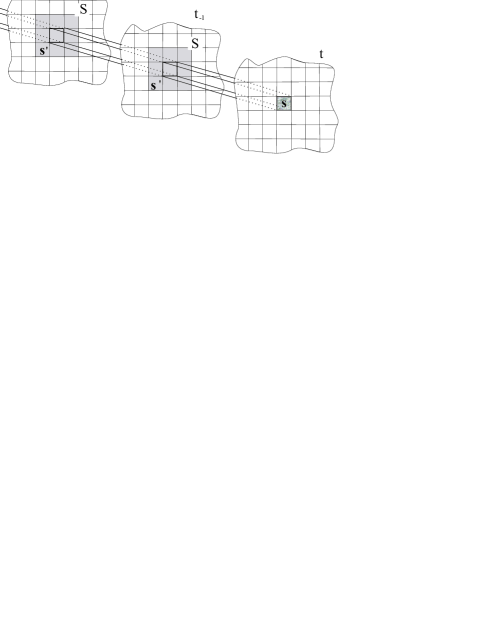
Figure 1: Illustration of point ${\bf s}$ and its surroundings ${\bf s}^{\prime}\in{\cal S}$. The future distribution of field ${\bf\varphi}$ (${\bf s}$) is located in plane $t_{+1}$, while the surrounding points ${\bf s}^{\prime}\in{\cal S}$, which represent the past distribution of field, are located in planes $t$, $t_{-1}$, $t_{-2}$…

The source of information for modeling the field generator is a field record containing joint sample pairs ${\bf\varphi}({\bf s})$ and ${\bf\varphi}({\bf s^{\prime}}\in{\cal S})$. These joint sample pairs form a sample vector ${\bf V}_{i}({\bf s})=({\bf\varphi}_{i}({\bf s}),{\bf\varphi}_{i}({\bf s}^{\prime}\in{\cal S}))$. To make further derivation more transparent, the past field distribution ${\bf\varphi}_{i}({\bf s^{\prime}})$ and the future field distribution ${\bf\varphi}_{i}({\bf s})$ will be denoted by ${\bf x}_{i}$ and ${\bf y}_{i}$, respectively. Hence ${\bf V}_{i}({\bf s})=({\bf y}_{i},{\bf x}_{i})$.

The samples ${\bf V}_{i}$ are interpreted as random variables and can therefore be used to express the joint probability distribution function (PDF) by the kernel estimator [14]

$$f_{N}({\bf V})=\frac{1}{N}\sum_{i=1}^{N}\psi({\bf V}-{\bf V}_{i},\sigma),$$ (2)

in which $\psi$ denotes an acceptable kernel function such as the Gaussian function $\psi(x-x_{i},\sigma)=1/(\sqrt{2\pi}\sigma){\rm exp}(-(x-x_{i})^{2}/2\sigma)$ and $N$ is the number of sample pairs.

Once the samples from the field record have been taken, the question of how to determine the optimal predictor becomes relevant. We consider as an optimal predictor of the future field distribution ${\bf y}$ from a given value ${\bf x}$ the value ${\bf\hat{y}}$ at which the mean square prediction error is minimal:

$${\rm E}[({\bf y}-{\bf\hat{y}})^{2}|x]={\rm min}({\bf\hat{y}}).$$ (3)

Here ${\rm E}[\,\,]$ denotes averaging over all points in a field record at a given time $t$. The solution of Eq. (3) yields together with PDF from Eq. (2) the conditional average estimator

$${\bf\hat{y}}({\bf x})=\frac{\sum_{i=1}^{N}{\bf y}_{i}\psi({\bf x}-{\bf x}_{i},\sigma)}{\sum_{j=1}^{N}\psi({\bf x}-{\bf x}_{j},\sigma)}=\sum_{i=1}^{N}{\bf y}_{i}C_{i}({\bf x}),$$ (4)

where coefficients of the expansion $C_{i}({\bf x})$ represent basis functions that measure the similarity between the temporary vector ${\bf x}$ and vector ${\bf x}_{i}$ from the field record. The conditional average estimator described by Eq. 4 represents a radial basis function neural network in which the recorded data ${\bf x}_{i},{\bf y}_{i}$ represent the memorized contents of neurons, ${\bf x}$ and ${\bf\hat{y}}({\bf x})$ are the input and the output of the network, while the basis functions $C_{i}({\bf x})$ correspond to activation functions of neurons. Since $\sum_{i=1}^{N}C_{i}({\bf x})=1$, the conditional average estimator represents a normalized RBFNN. In this function, the parameter $\sigma$ can be interpreted as the width of receptive fields of neurons.

II-B Quality of predictor

Working towards optimal modeling of future field distributions requires a quantitative estimation of modeling quality. We therefore introduce a testing field ${\bf y}$ and define the prediction quality $Q$, based upon the difference between the predicted field ${\bf\hat{y}}$ and the testing field ${\bf y}$ as:

$$Q=1-\frac{{\rm E}[({\bf\hat{y}}-{\bf y})^{2}]}{{\rm E}[({\bf\hat{y}}-{\bf\hat{\bar{y}}})^{2}]+{\rm E}[({\bf y}-{\bf\bar{y}})^{2}]}.$$ (5)

Here ${\bf\hat{\bar{y}}}$ and ${\bf\bar{y}}$ stand for the average values of predicted field ${\bf\hat{y}}$ and testing field ${\bf y}$, i.e., ${\rm E}[{\bf\hat{y}}]={\bf\hat{\bar{y}}}$ and ${\rm E}[{\bf y}]={\bf\bar{y}}$. A perfect prediction ${\bf\hat{y}}={\bf y}$ yields $Q=1$, while uncorrelated ${\bf\hat{y}}$ and ${\bf y}$ result in $Q=0$.

II-C Prediction of field evolution

The prediction process consists of three steps:

1. Learning, that corresponds to setting up the basis of joint sample pairs $({\bf\varphi}_{i}({\bf s}),{\bf\varphi}_{i}({\bf s}^{\prime}\in{\cal S}))$ = $({\bf x}_{i}$, ${\bf y}_{i})$ from the field record,

2. predicting the field ${\bf\hat{y}}$ by using the conditional average estimator from Eq. (4),

3. and, if the testing field exists, comparing predicted field with testing field and calculating prediction quality $Q$.

In order to achieve the highest quality of prediction for the process, answers to the following crucial questions are needed:

• How to find the surrounding ${\cal S}$ of a given point ${\bf s}$, which gives the best prediction of field ${\bf\hat{\varphi}}({\bf s})$ at this point?

• How to determine an optimal number of joint sample pairs $({\bf\varphi}_{i}({\bf s}),{\bf\varphi}_{i}({\bf s}^{\prime}\in{\cal S}))$ = $({\bf x}_{i}$, ${\bf y}_{i})$?

These questions will be addressed in the following chapters.

III Time evolution of melt pool

Characteristic dynamic properties of laser welding process in space and time can be experimentally obtained by recording the surface optical activity of the melt pool. With respect to the energy supplied to the material, various dynamic regimes of the welding process can be distinguished. In Fig. 2 visual records of two different welding regimes are shown, a deep welding regime (a) and a heat conduction welding regime (b). In the following discussion, only the deep welding regime is considered.

Figure 2: Time series of laser welding records for two different welding regimes: (a) a deep welding regime , and (b) a heat conduction welding regime. The next time-step images denoted by ? are unknown and must be predicted.

Dynamics of the welding regime are here represented by a record of 1000 images of size 32 $\times$ 32 points in space with sampling time 1/220 s. This experimental record forms a three-dimensional field of light intensity ${\bf\varphi}$(${\bf s}={\bf r},t$) in two-dimensional space $\{(r_{x,i},r_{y,i});i=1,..32,j=1..32\}$ and time $\{t_{k};k=1..1000\}$. Due to local energy supply, the field is non-homogeneous in space. Consequently, we model its evolution locally at each spatial point separately. A model of field evolution, i.e., the learning sample is formed from the first 800 images. We then predict the time evolution of the field and compare it with the next 200 images, which represent the testing sample. Based on the quality $Q$ of these predicted images, we optimize our prediction procedure, i.e., and define the structure of the surroundings ${\cal S}$, and the optimal number of joint sample pairs $N$ and parameter $\sigma$.

III-A Optimal value of parameter $\sigma$

Parameter $\sigma$ in the conditional average estimator ${\bf\hat{y}}$ (Eq. (4)) was to this point left undetermined. However, as shown in Fig. 3, obtained for the deep welding regime, the quality of prediction depends on the value of $\sigma$. The learning sample consisted of 800 images and the surrounding of predicted field distribution in point ${\bf s}=({\bf r},t)$ was taken to be just one neighboring point with the same space coordinate and the time coordinate being one step behind ${\bf s}^{\prime}=({\bf r},t_{-1})$. Based on the learning sample, ten images from the testing interval have been predicted and compared with the corresponding images from the testing field. The value $Q$ shown in Fig. 3 is the average quality of these ten images.

As Fig. 3 shows, the quality exhibits a strong $\sigma$ dependence at the beginning of the interval, and reaches its largest value for $\sigma$ approximately equal to 4. For larger values, it becomes a weakly decreasing function of $\sigma$. Since the optimal quality is reached for $\sigma\approx 4$, this value is used in our further calculations.

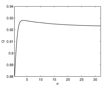
Figure 3: Dependence of prediction quality $Q$ on the value of parameter $\sigma$ from conditional average estimator ${\bf\hat{y}}$. Surrounding set ${\cal S}$ is taken to be only one point with the same spatial position and a neighboring position in time. Number of learning images in the learning field is set to 800.

As shown in Eq. (4), prediction of the field distribution at a given point is determined on the basis of similarity between the field distribution surrounding this point and the field distribution in surrounding points taken from the learning field. If we keep in mind that the parameter $\sigma$ defines the width of the Gaussian kernel function $\psi$ (see comment to Eq. 2), we can conclude, that for very small $\sigma$, only those joint sample pairs from the learning field which have a field distribution in the surrounding points (${\bf x_{i}}$) very similar to the field distribution in the surroundings of the point to be predicted (${\bf x}$) contribute to the predicted value of the field. On the other hand, for larger $\sigma$ those joint sample pairs with larger difference ${\bf x}-{\bf x_{i}}$ also contribute to the prediction of ${\bf\hat{y}}$. In the limit of large $\sigma$, almost all joint sample pairs contribute equally to ${\bf\hat{y}}$.

III-B Optimal number of joint sample pairs

If the prediction of welding pool images is to be part of a laser welding control system, the prediction operation has to be performed in the shortest time interval possible. Since the number of operations needed to predict a field distribution in a given point increases linearly with the number of joint sample pairs (see Eq. 4), it is necessary to find the smallest number of joint sample pairs which is still able to give predicted images of good quality.

In Fig. 4 we show the dependence of the quality of prediction on the number of images $N$ defining the learning field. As in the case of Fig. 3, the surrounding of the predicted field distribution in point ${\bf s}=({\bf r},t)$ was taken to be just one neighboring point with the same space coordinate and the time coordinate being one step behind ${\bf s}^{\prime}=({\bf r},t_{-1})$. Parameter $\sigma$ is set to 4. Again $Q$ is taken to be the average quality of ten predicted images, which were compared with the corresponding images from the testing field.

As one can see from Fig. 4, $Q$ increases rather strongly with small values of $N$ ($N<400$), while for $N>600$ an increase in $N$ does not result in a significant improvement of prediction quality. Therefore, in further calculations we apply $N=600$.

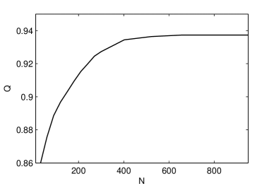
Figure 4: Dependence of prediction quality $Q$ on number of images defining the learning field. The surrounding set ${\cal S}$ is taken to be only one point with the same spatial position and a neighboring position in time. Parameter $\sigma$ is set to 4.

III-C Choosing the surrounding ${\cal S}$

Our next goal is to find an optimal structure of RBFNN which yields the best quality of prediction in the shortest time interval. The structure of surrounding set ${\cal S}$ plays an important role in this optimization process since each additional point in the surrounding increases the dimensionality of vectors ${\bf x}_{i}$ and therefore the time needed to predict the field distribution in a given point. Our task is to find the smallest surrounding of point ${\bf s}$, which results in high prediction quality.

In Fig. 5 the prediction quality is presented for various selections of surrounding set ${\cal S}$. Parameters $N$ and $\sigma$ are 600 and 4, respectively. As before, $Q$ represents the average quality of ten predicted images which were compared with the corresponding images from the testing field. All the member points of the first six surrounding sets in the diagram lie in the plane $t_{-1}$. Member points of other surrounding sets lie in several planes. For each of these, only those planes containing the member points are plotted..

As can be seen in Fig. 5, the smallest surrounding sets give the best quality of prediction - see sets Nr. 1-3 and 7-10. If more points belonging to the same time-plane are added to ${\cal S}$, prediction quality is decreased- compare, for example sets Nr. 1 and Nr. 6 or Nr. 14 and Nr. 15. In contrast, surrounding sets containing points from two planes, $t_{-1}$ and $t_{-2}$, give a slightly better $Q$ than sets containing only points from $t_{-1}$ - compare for example sets Nr. 1 and Nr. 7. However, an addition of multiple time-planes reduces the quality (see set Nr. 12).

As the best quality is obtained for set Nr. 7, this surrounding set is considered optimal in further calculations. We would like to stress, that in Fig. 5 only those surrounding sets which seemed to have the potential to give the best quality were taken into account. The optimal structure of ${\cal S}$ was chosen on the basis of selected sets. To be sure that the chosen structure was really optimal, it is necessary to calculate the prediction quality of all the subsets containing all combinations of neighboring points. Since the number of points in our learning set is 32$\times$32$\times$600, a calculation of $Q$ for all sets would become a computationally prohibitive task.

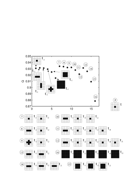
Figure 5: Dependence of prediction quality $Q$ (*) on the structure of the surrounding set ${\cal S}$. Parameters are $N=600$ and $\sigma=4$. The netlike patterns (1-16) describe the position of surrounding points, while the netlike pattern denoted by P describes the position of prediction point ${\bf s}$. In the netlike patterns, only those time planes which contain points from ${\cal S}$ are plotted.

III-D Optimal prediction of melt pool evolution

After determining the optimal parameters of our RBFNN model, we next show the discrepancy between the predicted images of the laser welding melt pool and the corresponding images from the testing field. In Fig. 6 we therefore present predicted laser welding images and corresponding images from the testing field for the optimal structure of RBFNN. Parameters are $N=600$, and $\sigma=4$, while the surrounding set ${\cal S}$ has only two member points, both having the same spatial position as the predicted point, but neighboring positions in time. Since the quality of prediction is 0.93 (see Fig. 5), a very good similarity between the predicted and corresponding image from the testing field is expected. Comparison of predicted images and images from the testing field in Fig. 6 indeed exhibits a good resemblance. However, we would like to draw attention to surface smoothness. As can be seen, the predicted surface is smoother than the original surface. This can be easily understood if the origin of prediction of images in the conditional average estimator (Eq. 4) is taken into account. Predicted ${\bf\hat{y}}$ is therefore a weighted average of all those ${\bf y}_{i}$, for which ${\bf x}_{i}$ is similar to ${\bf x}$. Consequently, the surface roughness is diminished due to conditional averaging.

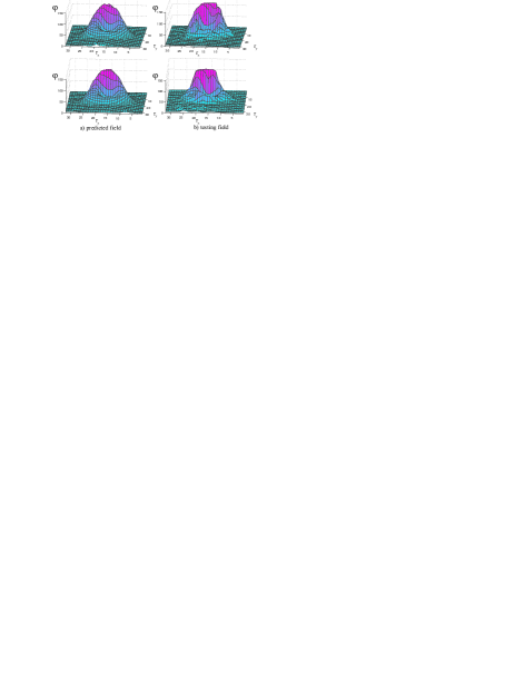
Figure 6: Comparison of predicted melt pool images (a) with corresponding images from the testing field (b) for two randomly chosen testing records. $\varphi$ stands for field, $r_{x}$ and $r_{y}$ denote spatial coordinates of the record. Parameters are $N=600$ and $\sigma=4$. The surrounding set ${\cal S}$ has only two member points, both having the same spatial position (${\bf r}$) as the predicted point ${\bf s}$=(${\bf r}$,t), but different neighboring positions in time, i.e., $t_{-1}$ and $t_{-2}$.

IV Conclusion

Time evolution of multi-dimensional fields is usually obtained by solving a system of partial differential equations. However, if the only source of information is a record of the field, a neural network can successfully replace differential equations by extracting field evolution properties from the recorded data. Neural-network-like structures are also expected to be the working algorithm of living organisms’ intelligence. In the same way as neural networks, living organisms predict the evolution of events in their surroundings solely on the basis of recorded data. It could be conjectured that this operation is probably performed by extracting simple evolution laws from recorded data.

In this paper we show how to optimize a statistical modeling of a field generator performed by the normalized RBFNN, to efficiently learn spatiotemporal dynamics of multi-dimensional fields. In our experimental approach, all information about process dynamics is contained in a measured space-time record of the characteristic variable. To extract the model of field evolution from the corresponding discrete sample data, we employ a non-parametric approach, following a state-space reconstruction technique. The basis of state-space reconstruction is the formation of sample vectors which are composed of past and future field distributions. We assume that the field distribution in a given spatiotemporal point ${\bf s}$ is correlated with the field distribution in the spatiotemporal surroundings of this point, ${\cal S}$. The prediction of field distribution in ${\bf s}$ is then accomplished as a mapping relation between the field distribution in the surroundings ${\cal S}$ and field distribution in ${\bf s}$.

Since the optimization of the state-space reconstruction technique also requires a quantitative measure of the prediction quality, we introduce the quality estimator $Q$, which incorporates the difference between the predicted field and the corresponding testing field. We consider as a proper set of model parameters those values at which the prediction quality achieves a maximum. This strategy is used here to find a proper value of parameter $\sigma$ and the structure of the surrounding ${\cal S}$ utilized in the prediction process. Generally, an estimation of the proper number of sample points must also consider the complexity of the experiments, which is numerically demanding in a multidimensional case [18]. Consequently, we also specify here the proper number $N$ based upon the analysis of prediction quality.

We demonstrate the proposed method of modeling of the properties of the laser-heated melt pool. For this purpose, we employ non-parametric statistical modeling of field evolution on a spatiotemporal record of the melt pool of the laser welding process. The major part of the field record is used for learning, while the minor part of the record serves for testing. We show how to construct the set of joint sample pairs containing past and future values of field distributions and pay special attention to the structure of these sample pairs. We also present the optimal structure of sample vectors, which gives the highest resemblance between predicted images and images from the testing field and has a small number of member points in order to make the prediction algorithm work quickly.

References

- [1] E. Govekar, J. Gradišek, I. Grabec, M. Geisel, A. Otto, M. Geiger, ”On characterization of CO2 laser welding process by means of light emitted by plasma and images weld pool”, in Third Int. Symp: Investigation of Non-linear Dynamics Effects in Production Systems (Cottbus, Germany), 2000.
- [2] E. Govekar, J. Gradišek, I. Grabec, M. Geisel, A. Otto, M. Geiger, ”Influence of feed rate on dynamics of laser welding process” in Second Int. Symp: Investigation of Non-linear Dynamics Effects in Production Systems (Aachen, Germany), 1999.
- [3] M. Casdagli, S. Eubank, ”Nonlinear Modeling and Forcasting”, Santa Fe Institute: Addison-Wesley, 1992.
- [4] H. D. I. Abarbanel, R. Brown, J. J. Sidorowich, L. S.Tsmiring, ”The analysis of observed chaotic data in physical systems”,Rev. Mod. Phys. Vol. 65, pp.1331-1392, 1993.
- [5] E. J. Kosterlich, T. Schreiber, ”Noise reduction in chaotic time-series data: A survey to common methods ”,Phys. Rev. E Vol. 48, pp.1752-1763, 1993.
- [6] H. Kantz, T. Schreiber, ”Nonlinear Time Series Analysis”, Cambridge University Press, 1997.
- [7] S. Sigert, R. Friedrich, J. Peinke, ”Analysis of data sets of stochasitc systems”, Phys. Lett. A Vol. 243, pp.275-289, 1998.
- [8] D. M. Rubin, ”Use of forecasting signatures to hlep destinguish periodicity, randomness, and chaos in ripples and other spatial patterns”, Chaos Vol. 2, pp.525-535, 1992.
- [9] I. Grabec, S. Mandelj, ”Continuation of chaotic fields by RBFNN”, in Bilological and Artificial Computation: From Neuroscience to Technology: Proc., eds. J. Mira, R. Moreno-Diaz, J. Cebestany, Lecture Notes in Computer Science (Springer-Verlag, Berlin), Vol. 1240, pp.597-606, 1997.
- [10] S. Ørstavik, J. Stark, ”Reconstruction and cross-prediction in coupled map lattices using spatiotemporal embedding techniques”, Phys. Lett. A Vol. 247, pp.145-160, 1998.
- [11] U. Parlitz, C. Merkwirth, ”Prediction of spatiotemporal time series based on reconstructed local states”, Phys. Rev. Lett. Vol. 84, pp.1890-1893, 2000.
- [12] S. Mandelj, I. Grabec and E. Govekar, ”Statistical modeling of stochastic surface profiles”, CIRP-J. Manuf. Syst, Vol. 30, pp 281-287, 2000.
- [13] S. Mandelj, I. Grabec and E. Govekar, ”Nonparametric statistical modeling of spatiotemporal dynamics based on recorded data”, Int. Jour. Bifur. Chaos, Vol. 14, No. 6, pp 2011-2025, 2004.
- [14] R. O. Duda, P. E. Hart, ”Pattern Clasification and Scene analysis”, J. Wiley and Sons, New York, Chap. 4. 1997.
- [15] H. U. Voss, M. J. Bünner, M. Abel, ”Identification of continuous, spatiotemporal systems”, Phys. Rev. E Vol. 57, pp.2820-2823, 1998.
- [16] M. Bär, R. Hegger, H.Kantz, ”Fitting partial differential equations to space-time dynamics”, Phys. Rev. E Vol. 59, pp.337-342, 1999.
- [17] H. U. Voss, P. Kolodner, M. Abel, J. Kurths, ”Amplitude equations from spatiotemporal binary-fluid convection data”, Phys. Rev. Lett Vol. 83, pp.3422-3425, 1999.
- [18] I. Grabec, ”Extraction of Physical Laws from Joint Experimental Data,” Eur. Phys. J. B, vol. 48, pp. 279-289, 2005.