Shocks in nonlocal media

Abstract

We investigate the formation of collisionless shocks along the spatial profile of a gaussian laser beam propagating in nonlocal nonlinear media. For defocusing nonlinearity the shock survives the smoothing effect of the nonlocal response, though its dynamics is qualitatively affected by the latter, whereas for focusing nonlinearity it dominates over filamentation. The patterns observed in a thermal defocusing medium are interpreted in the framework of our theory.

Shock waves are a general phenomenon thoroughly investigated in disparate area of physics (fluids and water waves, plasma physics, gas dynamics, sound propagation, physics of explosions, etc.), entailing the propagation of discontinuous solutions typical of hyperbolic PDE models Whitman74 ; Liberman86 . They are also expected in (non-hyperbolic) universal models for dispersive nonlinear media, such as the Korteweg-De Vries (KdV) and nonlinear Schrödinger (NLS, or analogous Gross-Pitaevskii) equations, since hydrodynamical approximations of such models hold true in certain regimes (typically, in the weakly dispersive or strongly nonlinear case) gp ; wkb ; Kamchatnov02 . However, in the latter cases, no true discontinuous solutions are permitted. The general scenario, first investigated by Gurevich and Pitaevskii gp , is that dispersion regularizes the shock, determining the onset of oscillations that appear near wave-breaking points and expand afterwards. This so-called collisionless shock has been observed for example in ion-acoustic waves Taylor70 , or wave-breaking of optical pulses in a normally dispersive fiber Grischkowsky89 , and recently in a Bose-Einstein condensate with positive scattering length Perez-Garcia04 .
In this Letter we investigate how nonlocality of the nonlinear response affects the formation of a collisionless shock in a system ruled by a NLS model. In fact nonlocality plays a key role in many physical systems due to transport phenomena and finite range interactions (e.g. as in Bose-Einstein condensation), and can be naively thought to smooth and eventually wipe out steep fronts characteristic of shocks. More specifically, we place this problem in the context of nonlinear optics where nonlocality arises quite naturally in different media Wyller02 ; Conti ; Yakimenko05 ; Segev05 , studying the spatial propagation of a fundamental (gaussian TEM₀₀) laser mode subject to diffraction and nonlocal focusing/defocusing action (Kerr effect). In a defocusing and ideal (local and lossless) medium, high intensity portions of the beam diffract more rapidly than the tails leading, at sufficiently high powers, to overtaking and oscillatory wave-breaking similar (in 1D) to what observed in the temporal case . We find that, while shock is not hampered by the presence of (even strong) nonlocality, the mechanism of its formation as well as post-shock patterns are qualitatively affected by the nonlocality. Experimental results obtained with a thermal defocusing nonlinearity are consistent with our theory and shed new light on the interpretation of the thermal lensing phenomenon.
Importantly, our theory permits also to establish that nonlocality allows the shock to form also in the focusing regime where, contrary to the local case, it can prevails over filamentation or modulational instability (MI).

Theory We start from the paraxial wave equation obeyed by the envelope $A$ of a monochromatic field $E=(\frac{2}{c\epsilon_{0}n})^{1/2}A\exp(ikZ-i\omega T)$ ($|A|^{2}$ is the intensity)

$$i\frac{\partial A}{\partial Z}+\frac{1}{2k}\left(\frac{\partial^{2}A}{\partial X^{2}}+\frac{\partial^{2}A}{\partial Y^{2}}\right)+k_{0}\Delta nA=-i\frac{\alpha_{0}}{2}A\text{.}$$ (1)

where $k=k_{0}n=\frac{\omega}{c}n$ is the wave-number, and $\alpha_{0}$ the intensity loss rate. A sufficiently general nonlocal model can be obtained by coupling Eq. (1) to an equation that rules the refractive index change $\Delta n$ of nonlinear origin. Introducing the scaled coordinates $x,y,z=X/w_{0},Y/w_{0},Z/L$, and complex variables $\psi=A/\sqrt{I_{0}}$ and $\theta=k_{0}L_{nl}\Delta n$, where $L_{nl}=(k_{0}|n_{2}|I_{0})^{-1}$ is the nonlinear length scale associated with peak intensity $I_{0}$ and a local Kerr coefficient $n_{2}$ ($\Delta n=n_{2}|A|^{2}$), $L_{d}=kw_{0}^{2}$ is the characteristic diffraction length associated with the input spot-size $w_{0}$, and $L\equiv\sqrt{L_{nl}L_{d}}$, such model can be conveniently written as follows Conti

$$\displaystyle i\varepsilon\frac{\partial\psi}{\partial z}+\frac{\varepsilon^{2}}{2}\nabla^{2}_{\perp}\psi+\chi\theta\psi=-i\frac{\alpha}{2}\varepsilon\psi,$$ (2)

$$-\sigma^{2}\nabla^{2}_{\perp}\theta+\theta=|\psi|^{2},$$ (3)

where $\alpha=\alpha_{0}L$, $\nabla^{2}_{\perp}=\partial_{x}^{2}+\partial_{y}^{2}$, $\chi=n_{2}/|n_{2}|=\pm 1$ is the sign of the nonlinearity, and $\sigma^{2}$ is a free parameter that measures the degree of nonlocality. The peculiar dimensionless form of Eqs. (2-3) where $\varepsilon\equiv L_{nl}/L=\sqrt{L_{nl}/L_{d}}$ is a small quantity, highlights the fact that we will deal with the weakly diffracting (or strongly nonlinear) regime, such that the local $\sigma=0$ and lossless $\alpha=0$ limit yields a semiclassical Schrödinger equation with cubic potential ($\varepsilon$ and $z$ replace Planck constant and time, respectively). We study Eqs. (2-3) subject to the axi-symmetric gaussian input $\psi_{0}(r)=\exp(-r^{2})$, $r\equiv\sqrt{x^{2}+y^{2}}$, describing a fundamental laser mode at its waist. For $\varepsilon\ll 1$, its evolution can be studied in the framework of the WKB trasformation $\psi(r,z)=\sqrt{\rho(r,z)}\exp\left[i\phi(r,z)\right/\varepsilon]$ wkb . Substituting in Eqs. (2-3) and retaining only leading orders in $\varepsilon$, we obtain

$$\rho_{z}+\left[\frac{(D-1)}{r}\rho u+(\rho u)_{r}\right] = -\alpha\rho;\;\;u_{z}+uu_{r}-\chi\theta_{r}=0,$$

$$-\sigma^{2}\left(\theta_{rr}+\frac{D-1}{r}\theta_{r}\right)+\theta = \rho.$$ (4)

where $u\equiv\phi_{r}$ is the phase chirp, and $D=2$ is the transverse dimensionality. The 1D case described by Eqs. (4) with $D=1$ and $r\rightarrow x$ ($\partial_{y}=0$) illustrates the basic physics with least complexity. In the defocusing case ($\chi=-1$) for an ideal medium ($\sigma=\alpha=0$, $\theta=\rho$), Eqs. (4) are a well known hyperbolic system of conservation laws (Eulero and continuity equations) with real celerities (or eigenspeeds, i.e. velocities of Riemann invariants) $v^{\pm}=u\pm\sqrt{-\chi\rho}$, which rules gas dynamics ($u$ and $\rho$ are velocity and mass density of a gas with pressure $\propto\rho^{2}$). A gaussian input is known to develop two symmetric shocks at finite $z$ wkb . Importantly the diffraction, which is initially of order $\varepsilon^{2}$, starts to play a major role in the proximity of the overtaking point, and regularize the wave-breaking through the appearance of fast (wavelength $\sim\varepsilon$) oscillations which connect the high and low sides of the front and expand outwards (far from the beam center) gp . Such oscillations, characteristic of a collisionless shock, appear simultaneously in intensity and phase chirp ($u$) as clearly shown in Fig. 1(a,c).

In the nonlocal case, the index change $\theta(x)$ can be wider than the gaussian mode (for large $\sigma$) and the shock dynamics is essentially driven by the chirp $u$ with $\rho$ adiabatically following. This can be seen by means of the following approximate solution of Eqs. (4): considering that the equation for $\rho$ is of lesser order [$O(\epsilon)$], with respect to those for $\theta$ and $u$ [$O(1)$], we assume $\rho=\exp(-2x^{2})$ unchanged in $z$ and solve exactly the third of Eq. (4) for $\theta(x)$ (though derived easily, its full expression is quite cumbersome). Then, applying the theory of characteristics Whitman74 , the second of Eqs. (4) is reduced to the following ODEs, where dot stands for $d/dz$

$$\dot{x}=u\;;\;\dot{u}=\chi\theta_{x},$$ (5)

equivalent to the motion of a unit mass in the potential $V(x)=-\chi\theta$ with conserved energy $E=\frac{u(z)^{2}}{2}+V(x)$. The solution of Eqs. (5) with initial condition $x(0)=s,u(0)=0$ yields $x(s,z),u(s,z)$ in parametric form, from which overtaking is found whenever $u(x,z)$ (obtained by eliminating $s$) becomes a multivalued function of $x$ at finite $z=z_{s}$. The shock point corresponding to $|du/dx|\rightarrow\infty$ is found from the solution $u(x,z)$ displayed in Fig. 2(a) [ 2(b)], at positions $x=\pm x_{s}\neq 0$ (defocusing case) or $x_{s}=0$ (focusing case). The shock distance $z_{s}$ increases with $\sigma$ in both cases, as shown in Fig. 2(c).

We have tested these predictions by integrating numerically Eqs. (2-3). Simulations with $\chi=-1$ [see Fig. 1(b,d)] show indeed steepening and post-shock oscillations in the spatial chirp $u$, which are accompanied by a steep front in $\rho$ moving outward. The shock location in $x$ and $z$ is in good agreement with the results of our approximate analysis summarized in Fig. 2.

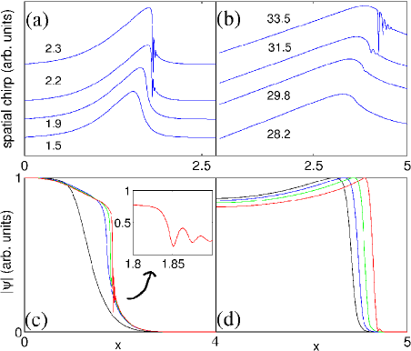
Figure 1: (Color online) 1D spatial profiles of phase chirp $u(x)$ (a-b) and amplitude $|\psi(x)|=\sqrt{\rho(x)}$ (c-d), as obtained from Eqs. (2-3) with $\varepsilon=10^{-3}$, $\alpha=0$, $\chi=-1$ (defocusing), and $\psi_{0}=\exp(-x^{2})$, for different $z$ as indicated: (a-c) local case, $\sigma^{2}=0$; (b-d) nonlocal case, $\sigma^{2}=5$.

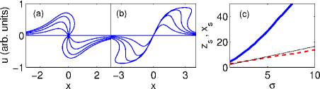
Figure 2: (Color online) (a) $u(x)$ for different $z$ and $\chi=1$ (focusing), $\sigma=1$; (b) as in (a) for $\chi=-1$ (defocusing); (c) shock distance $z_{s}$ ($\chi=-1$ bold solid, $\chi=1$ thin solid) and shock position $x_{s}$ in the defocusing case (dashed line).

Numerical simulations of Eqs. (2-3) validates also the focusing scenario. The field evolution displayed in Fig. 3(a) exhibits shock formation at the focus point ($x_{s}=0,z_{s}\simeq 8$, for $\sigma=5$) driven the phase whose chirp is shown in Fig. 3(b). This is remarkable because, in the local limit $\sigma=0$, the celerities become imaginary (the equivalent gas would have pressure decreasing with increasing density $\rho$), and no shock could be claimed to exist. In this limit, the reduced problem (4) is elliptic and the initial value problem is ill-posed focusing , an ultimate consequence of the onset of MI: modes with transverse (normalized) wavenumber $q<\Delta q$ grow exponentially with $z$, with both gain $g$ and bandwidth $\Delta q$ scaling as $1/\varepsilon$. However, the nonlocal response tends to frustrate MI (see also Refs. Wyller02 ; Conti ), as shown by standard linear stability analysis which yields $g=\sqrt{d(2\overline{\chi}-d)/\varepsilon^{2}}$ (we set $d\equiv\varepsilon^{2}q^{2}/2$ and $\overline{\chi}\equiv\chi/(1+\sigma^{2}q^{2})$), in turn implying a strong reduction of both gain and bandwidth for large $\sigma$. In order to emphasize the difference between the local and nonlocal regime, we contrast Fig. 3(a) with the analogous evolution [see Fig. 3(c)] obtained in the quasi-local limit ($\sigma^{2}=10^{-5}$), which appears to be clearly dominated by filamentation.

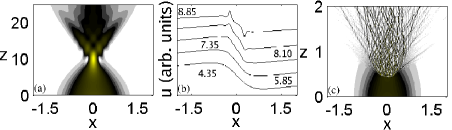
Figure 3: (Color online) Level plot of the intensity in the focusing case ($\chi=1$, $\varepsilon=0.01$): (a) nonlocal case ($\sigma^{2}=25$); (b) chirp profile for various $z$ for (a); (c) quasi-local case ($\sigma^{2}=10^{-5}$).

Thermal nonlinearity The physics of the defocusing case can be experimentally tested by exploiting thermal nonlinearities of strongly absorptive bulk samples, that we show below to fit our model. In this case, the system relaxes to a steady-state refractive index change $\Delta n=(dn/dT)\Delta T$, where $dn/dT$ is the thermal coefficient, and $\Delta T$ the local temperature change due to optical absorption. It is well known that this so-called thermal lens distorts a laser beam propagating in the medium tl ; rings ; Brochard97 . However, only perturbative approaches to the problem have been proposed (ray optics or Fresnel diffraction theory is applied after the lens profile is worked out from gaussian ansatz tl ), while the role of shock phenomena was completely overlooked.

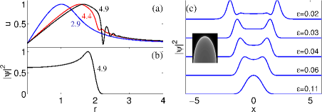
Figure 4: 2D evolution according to Eqs. (2-3) with $\sigma^{2}=1$, $\alpha=1$: (a) radial phase chirp at different $z$, as indicated, showing steepening and shock formation for $\varepsilon=10^{-2}$; (b) corresponding intensity profile $|\psi|^{2}$ (maximum scaled to unity) at $z=4.9$; (c) transverse intensity profile vs. $x$ (at $y=0$) at $z=1/(4\varepsilon)$ and different values of $\varepsilon$ ($\alpha_{0}=62$cm^-1, $\sigma=0.3$).

We assume that the temperature field $\Delta T=\Delta T_{\perp}(X,Y)$ obeys the following 2D heat equation

$$(\partial_{X}^{2}+\partial_{Y}^{2})\Delta T_{\perp}-C\Delta T_{\perp}=-\gamma|A|^{2}$$ (6)

where the source term account for absorption proportional to intensity through the coefficient $\gamma=\alpha_{0}/(\rho_{0}c_{p}D_{T})$, where $\rho_{0}$ the material density, $c_{p}$ the specific heat at constant pressure, and $D_{T}$ is the thermal diffusivity (see e.g. Brochard97 ). Eq. (6) has been already employed to model a refractive index of thermal origin in Ref. Yakimenko05 , and in Ref. Segev05 in the limit $C=0$ which is equivalent to consider the range of nonlocality (measured by $1/C$, see below) to be infinite. Starting from the 3D heat equation $\nabla^{2}\Delta T=-\gamma|A|^{2}$, the latter regime amounts to assume $\Delta T(X,Y,Z)=\Delta T_{\perp}(X,Y)$, which is justified when longitudinal changes in intensity $|A|^{2}$ are negligible as for solitary (invariant in $Z$) wave-packets in the presence of low absorption Segev05 . Viceversa, in the regime of strong absorption, we need to account for longitudinal temperature profiles that are known from solutions of the 3D heat equations to be peaked at characteristic distance $\hat{Z}$ in the middle of sample and decay to room temperature on the facets tl . Since highly nonlinear phenomena occurs in the neighborhood of $\hat{Z}$ where the index change is maximum, we can use a (longitudinal) parabolic approximation with characteristic width $L_{eff}(\sim L$) of the 3D temperature field $\Delta T(X,Y,Z)=\left[1-\frac{(Z-\hat{Z})^{2}}{2L_{eff}^{2}}\right]\Delta T_{\perp}(X,Y)$ and consequently approximate $\nabla^{2}\Delta T\simeq(\partial_{X}^{2}+\partial_{Y}^{2})\Delta T_{\perp}-L_{eff}^{-2}\Delta T_{\perp}$, so that the 3D heat equation reduces to Eq. (6) with $C=1/L_{eff}^{2}$. Following this approach, Eq. (6) coupled to Eq. (1) can be casted in the form of Eqs. (2-3) by posing $\theta=k_{0}L_{nl}|dn/dT|\Delta T_{\perp}$ and $\sigma^{2}=1/(Cw_{0}^{2})=L_{eff}^{2}/w_{0}^{2}$. The model reproduces the infinite range nonlocality for negligible losses ($L_{eff}\rightarrow\infty$); while for thin samples [$|(\partial_{X}^{2}+\partial_{Y}^{2})\Delta T_{\perp}|<<|L_{eff}^{-2}\Delta T_{\perp}|$], $L_{eff}$ can be related to the Kerr coefficient $n_{2}$ as

$$L_{eff}=\sqrt{\frac{|n_{2}|}{\gamma|dn/dT|}}=\sqrt{\frac{D_{T}\rho_{0}c_{p}|n_{2}|}{\alpha_{0}|dn/dT|}}$$ (7)

which establishes a link between the degree of nonlocality and the strength of the nonlinear response (similarly to other nonlocal materials Conti ).
Having retrieved the model Eqs. (2-3), let us show next that the scenario illustrated previously applies substantially unchanged in bulk (2D case) even on account for the optical power loss ($\alpha\neq 0$). An example of the general dynamics is shown in Fig. 4, where we report a simulation of the full model (2-3), with $\sigma^{2}=1$ and relatively large loss $\alpha=1$. In analogy to the 1D case, Fig. 4(a) clearly shows that the radial chirp $u=\phi_{r}$ steepens and then develop characteristic oscillations after the shock point ($z\simeq 6$, where $|\partial_{r}u|\rightarrow\infty$). Correspondingly the intensity exhibits also an external front which is connected to a flat central region with a characteristic overshoot [see Fig. 4(b)] corresponding to a brighter ring [inset in Fig. 4(c)]. For larger distances this structure moves outward following the motion of the shock. In the experiment such motion can be observed, at fixed physical lenght, by increasing the power, which amounts to decrease $\varepsilon$ while scaling $z$ and $\alpha$ accordingly ($z\propto 1/\varepsilon$, $\alpha\propto\varepsilon$), as displayed in Fig. 4(c) for $\sigma=0.3$.

As a sample of a strongly absorbing medium we choose a $1$ mm long cell filled with an acqueous solution of Rhodamine B ($0.6$ mM concentration). Our measurements of the linear and nonlinear properties of the sample performed by means of the Z-scan technique gives data consistent with the literature Sinha00 , and allows us to extrapolate at the operating vacuum wavelength of 532 nm, a linear index $n=1.3$, a defocusing nonlinear index $n_{2}=7\times 10^{-7}$ cm²W^-1, and $\alpha_{0}=62$ cm^-1. For our sample $D_{T}=1.5\times 10^{-7}$ m²s^-1, $\rho_{0}=10^{3}$ kg m^-3, $c_{p}=4\times 10^{3}Jkg^{-1}K^{-1}$ and $|dn/dT|=10^{-4}$ K^-1 ($\gamma\cong 10^{4}$ K W^-1), and exploiting Eq. (7) we estimate $L_{eff}\cong 10\mu$m ($L_{eff}<<L$ because of the strong absorption that causes strong heating of our sample near the input facet), and correspondingly the degree of nonlocality $\sigma\cong 0.3$. We operate with an input gaussian beam with fixed intensity waist $w_{0I}=w_{0}/\sqrt{2}=20~{}\mu$m ($L_{d}\cong 12$ mm) focused onto the input face of the cell. With these numbers, an input power $P=\pi w_{0I}^{2}I_{0}=200$ mW yields a nonlinear length $L_{nl}\cong 8~{}\mu$m ($L\cong 0.3$ mm), which allows us to work in the semiclassical regime with $\varepsilon\cong 0.025$. The radial intensity profiles together with the 2D patterns imaged by means of a $40\times$ microscope objective and a recording CCD camera are reported in Fig. 5. As shown the beam exhibits the formation of the bright ring whose external front moves outward with increasing power, consistently with the reported simulations. We point out that, at higher powers, we observe (both experimentally and numerically) that the moving intensity front leaves behind damped oscillations that correspond to inner rings of lesser brightness, as reported in literature rings . This, however, occurs well beyond the shock point that we have characterized so far.
In summary, the evolution of a gaussian beam in the strong nonlinear regime is characterized by occurence of collisionless (i.e., regularized by diffraction) shocks that survive the smoothing effect of (even strong) nonlocality. While experimental results support the theoretical scenario in the defocusing case, the remarkable result that the nonlocality favours shock dynamics over filamentation requires future investigation.

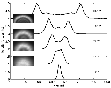
Figure 5: Radial profiles of intensity observed in the thermal medium for different input powers. The insets show the corresponding 2D output patterns.

References

- (1) G. B. Whitman, Linear and Nonlinear Waves (Wiley, New York, 1974);
- (2) L. D. Landau and E. M. Lifshitz, Fluid Mechanics (Pergamon, 1995); M. A. Liberman and A. L. Yelikovich, Physics of Shock Waves in Gases and Plasmas (Springer, Heidelberg, 1986).
- (3) A.V. Gurevich and L.P. Pitaevskii, Sov. Phys. JETP 38, 291 (1973); A.V. Gurevich and A. L. Krylov, Sov. Phys. JETP 65, 944 (1987).
- (4) J. C. Bronski and D. W. McLaughlin, in Singular Limits of Dispersive Waves, NATO ASI Series, Ser. B 320, pp. 21-28 (1994); M. G. Forest and K. T. R. McLaughlin, J. Nonlinear Science 7, 43 (1998); Y. Kodama, SIAM J. Appl. Math. 59, 2162 (1999). M. G. Forest, J. N. Kutz, and K. T. R. McLaughlin, J. Opt. Soc. Am. B 16, 1856 (1999).
- (5) A. M. Kamchatnov, R. A. Kraenkel, and B. A. Umarov, Phys. Rev. E 66, 036609 (2002).
- (6) R. J. Taylor, D.R. Baker, and H. Ikezi, Phys. Rev. Lett. 24, 206 (1970).
- (7) J. E. Rothenberg and D. Grischkowsky, Phys. Rev. Lett. 62, 531 (1989).
- (8) M. A. Hoefer, M. J. Ablowitz, I. Coddington, E. A. Cornell, P. Engels, and V. Schweikhard, Phys. Rev. A74, 023623 (2006). V. M. Perez-Garcia, V.V. Konotop, V.A. Brazhnyi, Phys. Rev. Lett. 92, 220403 (2004); B. Damski, Phys. Rev. A 69, 043610 (2004);
- (9) J. Wyller, W. Krolikowski, O. Bang, J. J. Rasmussen, Phys. Rev. E 66, 066615 (2002).
- (10) A. Yakimenko, Y. Zaliznyak and Y.S. Kivshar, Phys. Rev. E71, 065603(R) (2005).
- (11) C. Rotschild, O. Cohen, O. Manela, M. Segev and T. Carmon, Phys. Rev. Lett. 95, 213904 (2005).
- (12) C. Conti, M. Peccianti and G. Assanto, Phys. Rev. Lett. 91 073901 (2003); Phys. Rev. Lett. 92 113902 (2004); C. Conti, G. Ruocco and S. Trillo, Phys. Rev. Lett. 95 183902 (2005).
- (13) P. D. Miller and S. Kamvissis, Phys. Lett. A 247, 75 (1998); J. C. Bronski, Physica D 152, 163 (2001).
- (14) C. A. Carter and J. M. Harris, Appl. Opt. 23, 476 (1984); S. Wu and N. J. Dovichi, J. Appl. Phys. 67, 1170 (1990); F. Jürgensen and W. Schröer, Appl. Opt. 34 41 (1995).
- (15) C. J. Wetterer, L. P. Schelonka, and M. A. Kramer, Opt. Lett. 14, 874 (1989).
- (16) P. Brochard, V. Grolier-Mazza and R. Cabanel, J. Opt. Soc. Am. B 14, 405 (1997).
- (17) S. Sinha, A. Ray, and K. Dasgupta, J. Appl. Phys. 87, 3222 (2000).