Dramatic Variability of X-ray Absorption Lines in the Black Hole Candidate Cygnus X-1

Chulhoon Chang¹¹affiliation: Email: chang40@physics.purdue.edu, cui@physics.purdue.edu and Wei Cui¹¹affiliation: Email: chang40@physics.purdue.edu, cui@physics.purdue.edu Department of Physics, Purdue University, West Lafayette, IN 47907

Abstract

We report results from a 30 ks observation of Cygnus X-1 with the High Energy Transmission Grating Spectrometer (HETGS) on board the Chandra X-ray Observatory. Numerous absorption lines were detected in the HETGS spectrum. The lines are associated with highly ionized Ne, Na, Mg, Al, Si, S, and Fe, some of which have been seen in earlier HETGS observations. Surprisingly, however, we discovered dramatic variability of the lines over the duration of the present observation. For instance, the flux of the Ne X line at 12.14 Å was about $5\times 10^{-3}$ photons cm^-2 s^-1 in the early part of the observation but became subsequently undetectable, with a 99% upper limit of $0.06\times 10^{-3}$ photons cm^-2 s^-1 on the flux of the line. This implies that the line weakened by nearly two orders of magnitude on a timescale of hours. The overall X-ray flux of the source did also vary during the observation but only by 20–30%. For Cyg X-1, the absorption lines are generally attributed to the absorption of X-rays by ionized stellar wind in the binary system. Therefore, they may provide valuable diagnostics on the physical condition of the wind. We discuss the implications of the results.

binaries: general — black hole physics — stars: winds,outflows — stars: individual (Cygnus X-1) — X-rays: binaries

1 Introduction

Cygnus X-1 is the first dynamically-determined black hole system (Webster & Murdin 1972; Bolton 1972). It is in a binary system with a massive O9.7 Iab supergiant, and the orbital period was determined optically to be 5.6 days. Cyg X-1 is thus intrinsically different from the majority of known black hole candidates (BHCs) whose companion stars are much less massive (see review by McClintock & Remillard 2006). Curiously, those that have a high-mass companion (including Cyg X-1, LMC X-1 and LMC X-3) are all persistent X-ray sources, while those that have a low-mass companion are exclusively transient sources. Perhaps, stellar wind from the companion star plays a significant role in this regard (Cui, Chen, & Zhang 1997).

Unlike transient BHCs, in which mass accretion is mediated by the companion star overfilling its Roche-lobe, Cyg X-1 is thought to be a wind-fed system. In this case, however, the wind is thought to be highly focused toward the black hole, because the companion star is nearly filling its Roche lobe (Gies & Bolton 1986). The observed orbital modulation of the X-ray flux (Wen et al. 1999; Brocksopp et al. 1999a) has provided tentative evidence for wind accretion, because it is probably caused by varying amount of absorption through the wind (Wen et al. 1999). On the other hand, it is generally believed that an accretion disk is also present, based on the presence of an ultra-soft component, as well as Fe K_α emission line in the X-ray spectrum (e.g., Ebisawa et al. 1996; Cui et al. 1998).

Cyg X-1 is probably still the most studied BHC. It is a fixture in the target list for all major X-ray missions. Much has been learned from modeling the X-ray continuum of the source, as well as from studying its X-ray variability. A recent development is the availability of high-resolution X-ray data, which may shed further light on the accretion process and the environment within the binary system. Cyg X-1 has been observed on many occasions with the High Energy Transmission Grating Spectrometer (HETGS) on board the Chandra X-ray Observatory and the Reflection Grating Spectrometer on board the XMM-Newton Observatory. The high-resolution spectra have revealed the presence of numerous absorption lines that are associated with highly ionized material (Marshall et al. 2001; Schulz et al. 2002; Feng et al. 2003; Miller et al. 2005).

In this work, we report the detection of absorption lines, some of which have been seen previously but are much stronger here, and, more surprisingly, the discovery of dramatic variability of the lines, based on data from our HETGS/Chandra observation of Cyg X-1 during its 2001 state transition. The fluxes of some of the lines varied by nearly two orders of magnitude over the duration of the observation, while the overall flux of the source varied only mildly.

2 Observations and Data Reduction

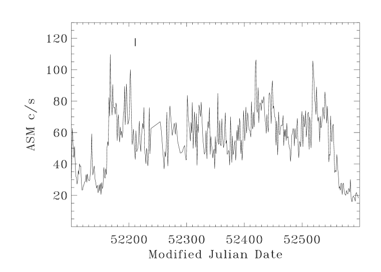
Cyg X-1 made a rare transition between the low-hard state and the high-soft state, as seen by the All-Sky Monitor (ASM) on the Rossi X-ray Timing Explorer (RXTE), about five years after a similar episode in 1996 (Cui et al. 1997a and 1997b). Figure 1 shows the ASM light curve that covers the entire period. In this case, the flux of the source stayed high for $\sim$ 400 days, about twice as long as in 1996. Otherwise, the two episodes are very similar, including the flux levels of the two states, prominent X-ray flares in both states, and rapid transitions.

Triggered by the ASM alert, the source was observed from 2001 October 28 16:13:52 to October 29 00:33:52 (UT) with the HETGS on Chandra (ObsID #3407). The HETGS consists of two gratings: Medium Energy Grating (MEG) and High Energy Grating (HEG). After passing the gratings, the photons are recorded and read out with the spectroscopic array of the Advanced CCD Imaging Spectrometer (ACIS). To avoid photon pile-up in the dispersed events, we chose to run the ACIS in continuous-clocking (CC) mode. We also applied a spatial window around the aim point to accept every $10^{th}$ event in the zeroth order, to prevent telemetry saturation yet still have a handle on the position of the zeroth-order image for accurate wavelength calibration.

The Chandra data were reduced and analyzed with the standard CIAO analysis package (version 3.2). Following the CIAO 3.2 Science Threads¹¹1See http://asc.harvard.edu/ciao3.2/threads/index.html, we prepared and filtered the data, produced the Level 2 event file from the Level 1 data products, constructed the light curves, and made the spectra and the corresponding response matrices and auxilliary response files (ARFs). We did have to work around a problem related to the use of maskfile for the CC-mode data, when we were making the ARFs. The solution is now included in the CIAO 3.3 Science Threads. To verify wavelength calibrations, we compared the plus and minus orders and found good agreement on the position of prominent lines. We did not subtract background from either the light curves or the spectra, because it is not obvious how to select background events from the CC-mode data. For a bright source like Cyg X-1, however, we expect the effects to be entirely negligible.

In coordination with the Chandra observation, we also observed Cyg X-1 with the Proportional Counter Array (PCA) and High Energy X-ray Timing Experiment (HEXTE) detectors on board RXTE. The PCA and HEXTE covers roughly the energy ranges of 2–60 keV and 15-250 keV, respectively. In this work, we made use of the combined broad spectral coverage of the two detectors to constrain the X-ray continuum more reliably. The RXTE observation was carried out in six short segments, with exposure times of 1–3 ks. The data were reduced with the standard HEASOFT package (version 5.2), along with the associated calibration files and background models. We followed the usual procedures²²2See http://heasarc.gsfc.nasa.gov/docs/xte/recipes/cook_book.html in preparing, filtering, and reducing the data, as well as in deriving light curves and spectra from the standard-mode data. While the HEXTE background was directly measured from off-source observations, the PCA background was estimated based on the background model appropriate for bright sources.

3 Analysis and Results

3.1 Light Curves

Figure 2 shows the Chandra light curve of Cyg X-1 that is made from the MEG first-order data (with plus and minus one orders coadded). For comparison, we have over-plotted the average count rate of PCU #2 for each of the RXTE exposures. The agreement is quite good. Besides the rapid flares and other short-term variability that are expected in Cyg X-1, the source also varies significantly on a timescale of hours. The MEG count rate rises from a baseline level of roughly 170 counts s^-1 to a peak of roughly 220 counts s^-1 within 3–4 hours and quickly goes back down to the baseline level. We somewhat arbitrarily divided the light curve into two time periods (which are labeled as Period I and Period II in Fig. 2) for subsequent analyses.

3.2 High-Resolution Spectroscopy

We analyzed and modeled the HETGS spectra in ISIS (version 1.2.9) (Houck & Denicola 2000)³³3See also http://space.mit.edu/CXC/ISIS/. For this work, we focused only on the first-order spectra, because of the relatively poor signal-to-noise ratio of higher-order spectra. For both the MEG and HEG, we first co-added the plus and minus orders to produce an overall first-order spectrum, again following the appropriate CIAO 3.2 science threads. The resolution of the raw data is about 0.01 Å and 0.005 Å for the MEG and HEG, respectively, which represents a factor of 2 over-sampling of the instrumental resolution. We applied no further binning of the data. Each spectrum was broken into 3-Å segments for subsequent analyses. Each segment was fitted locally with a model that consists of a multi-color disk component and a power law for the continuum and negative or positive Gaussian functions for narrow absorption or emission features, with the interstellar absorption taken into account. Such a continuum model is typical of BHCs. However, the best-fit continuum differs among the segments or between the MEG and HEG, presumably due to remaining calibration uncertainties. Since we are only interested in using the Chandra data to study lines, we think that the adopted procedure is justified. We use the RXTE data to more reliably constrain the continuum.

One thing that one notices right away is the presence of many absorption lines in the high-resolution spectra. For this work, we consider a feature real if it is present both in the MEG and HEG data, with a significance of above 4 $\sigma$ . Figure 3 shows a portion of the MEG first-order spectrum for Period I, to highlight the lines detected. No absorption lines were found at wavelengths above 15 Å. We should point out that we also see the emission-like features at 6.74 Å and 7.96 Å, which most likely instrumental artifacts associated with calibration uncertainties around the Si K and Al K edges (Miller et al. 2005 and references therein). We have identified the absorption lines with highly ionized species of Ne, Na, Mg, Al, Si, S, and Fe, based mostly on the atomic data in Verner et al. (1996) and Behar et al. (2002), but also in ATOMDB⁴⁴4See http://cxc.harvard.edu/atomdb 1.3.1 for additional transitions.

The line identification process involves three steps: (1) a transition is considered a candidate if the theoretical wavelength is within 0.03 Å of the measured value; (2) in cases where multiple candidates exist based on (1), the most probably one (based both on the oscillator strength of the transition and the relative abundance of the element) is chosen; and (3) consistency check is made to avoid the identification of a line when more probable transitions of the same ion are not seen. The last step is critical. For instance, we initially associated the lines at 10.051 Å and 11.029 Å with Fe XVIII $2s^{2}2p^{5}$ – $2s^{2}2p^{4}6d$ and Fe XVII $2s^{2}2p^{6}$ – $2s2p^{6}4p$ , respectively, because, assuming solar abundances, they are expected to be stronger than Na XI $1s$ – $2p$ and Na X $1s^{2}$ – $1s1p$ , which were also viable candidates from Step 1. However, we did not detect other more probable transitions associated with Fe XVIII and Fe XVII, which made the identifications highly unlikely. We had to conclude that Fe is under-abundant by a factor of 2–3, at minimum, so that we could associate the lines with Na instead. If so, the line at 7.480 Å would more likely be associated with Mg XI $1s^{2}$ – $1s4p$ , as opposed to Fe XXIII $2s^{2}$ – $2s5p$ , which we initially identified. The problem with this is that we saw no hint of Mg XI $1s^{2}$ – $1s3p$ , which is more probable. Therefore, we had to conclude similarly that Mg is also under-abundant by at least a similar amount (but not by too much, as constrained by other Mg lines).

Table 1 show all of the absorption lines that we detected and identified. The flux and equivalent width (EW) of each line shown were derived from the best-fit Gaussian for the line, as well as the local continuum around the line for the latter. Note that in a few cases our identifications are different from those in the literature. They include: Fe XXII at 8.718 Å and Fe XXI at 9.476 Å (cf. Marshall et al. 2001; Miller et al. 2005); Fe XX at 10.12 Å, Na X at 11.0027 Å, and Fe XX at 12.82 Å (cf. Marshall et al. 2001); and Fe XXI 11.975 Å (cf. Miller et al. 2005). Only about half of the absorption lines that we detected have been seen previously in Cyg X-1 (Marshall et al. 2001; Schulz et al. 2002; Feng et al. 2003; Miller et al. 2005). Many of these lines are much stronger in our case. On the other hand, we detected nearly all of the reported absorption lines. The exceptions include: S XVI at 4.72 Å (Marshall et al. 2001; Feng et al. 2003), which is detectable only at the $3\sigma$ level in our case (and is thus not included in the table), Fe XIX at 14.53 Å (Miller et al. 2005), which is actually detectable at about the $4\sigma$ level here (but just misses our threshold), and Fe XIX at 14.97 Å and Fe XVIII at 16.01 Å (Miller et al. 2005), whose presence is not apparent in our data ( $<3\sigma$ ). Miller et al. (2005) also reported a line at 7.85 Å (Mg XI) but only at the $3\sigma$ level. The line can also be seen in our data at the $4\sigma$ level (but also just misses our threshold). Therefore, we already see some indication that the absorption lines in Cyg X-1 may be variable from a comparison of our results with those published.

Still, it is surprising that almost all of the absorption lines become undetectable in Period II. Figure 4 shows the MEG first-order spectrum for this time period, which can be directly compared to results in Fig. 3. The only exception is the line at 14.608 Å, which is detected with a significance of $5\sigma$ in Period II. We derived 99% upper limits on the flux and EW of each line seen in Period I but not in Period II. The results are also summarized in Table 1, for direct comparison. As an example, we examine the Ne X line at 12.1339 Å in the two periods. The integrated flux of the line is about $5\times 10^{-3}$ photons cm² s^-1 in Period I, while its 99% upper limit for Period II is only $0.06\times 10^{-3}$ photons cm² s^-1. Therefore, the line weakened by nearly two orders of magnitude in flux over a timescale of merely several hours. This is the first time that such dramatic variability of the lines has been observed in any BHC. While this is the most extreme case, other lines also show large variability (see Table 1).

To quantify the column density of each ion required to account for the corresponding absorption line detected and its variability, we carried out curve-of-growth analysis, following Kotani et al. (2000). The atomic data used in the analysis were again taken from Verner et al. (1996), Behar et al. (2002), and also ATOMDB 1.3.1 in some cases. The analysis assumes that the width of the lines is due entirely to thermal Doppler broadening. For resolved lines, we derived the characteristic temperature from the measured widths. For unresolved lines, on the other hand, we adopted a temperature that would lead to a line width equal to the resolution of the MEG (0.023 Å at FWHM). In these cases, therefore, the derived column density only represents a lower limit. The results are shown in Table 1. This explains why, e.g., the density of Ne X derived from the 12.144-Å line (which is unresolved) is significantly lower than that from the 10.245-Å line. Note, however, that the latter is much lower that that from the 9.727-Å line. We think that the inconsistency arises from the fact that the 9.727-Å line is likely a mixture of the Ne line and the Fe XIX line at 9.700 Å. Similar inconsistency is also apparent in a few other cases (see Table 1), which may originate similarly in line blending. It is also worth noting that most lines that we have analyzed fall on the linear part of the curve of growth. All resolved lines at wavelengths $\lambda>11.7$ Å are saturated; so is the unresolved line at 14.203 Å. To show the degree of variability, we also derived a 99% upper limit on the column density of each of the ions for Period II (assuming the same characteristic temperatures).

3.3 X-ray Continuum

We now use the RXTE data to constrain the X-ray continuum of Cyg X-1. Both the PCA and HEXTE data were used. For the PCA, we used only data from the first xenon layer of each PCU, which is most accurately calibrated. Consequently, the PCA spectral coverage is limited to roughly 2.5–30 keV. We relied on the HEXTE data to extend spectral coverage to higher energies. The PCA consists of five detector units, known as PCUs. Not all PCUs were always operating. For simplicity, we used only data from PCU #0 and PCU #2, which stayed on throughout the observation, in the subsequent modeling. We chose to derive a spectrum for each PCU separately, as well as for each of the two HEXTE clusters. Residual calibration errors were accounted for by adding 1% systematic uncertainty to the data. We also rebinned the HEXTE spectra to a signal-to-noise ratio of at least 3 in each bin. The individual spectra were then jointly fitted with the same model that includes a multi-color disk component, a broken power-law that rolls over exponentially beyond a characteristic energy, and a Gaussian, taking into account the interstellar absorption. We also multiply the model by a normalization factor that is fixed at unity for PCU #2 but is allowed to vary for other detectors, in order to account for any uncalibrated difference in the overall throughput among the detectors. The model fits the data well for all six segments in the sense that the reduced $\chi^{2}$ is near unity (with 169 degrees of freedom).

The spectral shape of Cyg X-1 varied little from one observation to the other. The best-fit photon indices are $\sim$ 2.1 and $\sim$ 1.7 below and above $\sim$ 10 keV. The roll-over energy stays at 20–21 keV and the e-folding energy roughly at 120–130 keV. Neither the disk component nor the absorption column density is well constrained by the data, due to the lack of sensitivity (and, to some extent, large calibration uncertainty) at low energies. The results can be compared directly with those of Cui et al. (1997a), who applied the same empirical model to the RXTE spectra of Cyg X-1 during the 1996 transition. It is quite apparent that the spectra here are significantly harder, implying that the source was certainly not yet in the true high-soft state (see Cui et al. 1997a and 1997b for discussions on the “settling period”). From the long-term ASM monitoring data, we can see that Cyg X-1 was brighter during our observation than during any of the earlier Chandra observations (Marshall et al. 2001; Schulz et al. 2002; Miller et al. 2005), but not as bright as during a later observation (Feng et al. 2003), when the high-soft state appears to have been reached.

3.4 Photoionization Modeling

To shed light on the physical properties of the absorber, we carried out a photo-ionization calculation with XSTAR version 2.1 kn3⁵⁵5See http://heasarc.gsfc.nasa.gov/docs/software/xstar/xstar.html. The underlying assumption is that the absorber is photo-ionized by the X-ray radiation from the vicinity of the black hole. The input parameters include the 0.5-10 keV luminosity ( $L_{x}=3.11\times 10^{37}$ erg s^-1, for a distance of 2.5 kpc), power-law photon index (2.1), both of which are based on results from modeling one of the RXTE spectra with an assumed $N_{H}$ value of $5.5\times 10^{21}$ cm^-2 (Ebisawa et al. 1996; Cui et al. 1998). We should note that it is in general risky to extrapolating the assumed power-law spectrum to lower energies, because it could severely over-estimate the flux there. For the lines of interest here, however, only ionizing photons with energies $>$ 1 keV contribute and the spectrum of those photons is described fairly well by a power law, because the effective temperature of the disk component is expected to very low (e.g., Ebisawa et al. 1996; Cui et al. 1998).

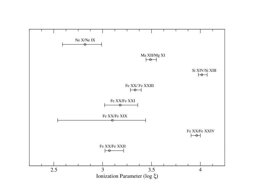
One of the outputs of the calculation is abundances of the ions of interest, as a function of the ionization parameter, $\xi=L_{x}/nr^{2}$ , where $n$ is the density of the absorber and $r$ is the distance of the absorber to the source of ionizing photons. Using these abundance curves, we could, in principle, constrain $\xi$ to a range that is consistent with the ratio of the densities of any two ions of an element. The challenge in practice is, as already mentioned, that many of the lines are likely a blend of multiple transitions (of comparable probabilities), which makes it difficult to reliably determine the densities. Nevertheless, we made an attempt at deriving such constraints with the resolved, non-mixed lines. Figure 5 summarizes the results. The intervals do not all overlap, which implies that no single value of $\xi$ could account for all the data. This is supported by the fact that we have detected all the lines that are expected for ionization parameters in the range of roughly $10^{2.5}$ – $10^{4.5}$ . If one assumes that the “absorbers” are thin shells along the line of sight and that they all have the same density, e.g., $n=10^{11}$ $cm^{-3}$ (see, e.g., Wen et al. 1999), one would have $10^{11}$ $cm$ $\lesssim r\lesssim$ $10^{12}$ $cm$ . Compared with the estimated the distance between the compact object and the companion star ( $\sim 1.4\times 10^{12}$ $cm$ ; LaSala et al. 1998), this would put the “absorbers” within the binary system. One should, however, take the results with caution, because of, e.g., gross over-simplification regarding the geometry of the “absorbers”.

4 Discussion

The observed dramatic variability of the absorption lines might be caused by a change in the degree of ionization in the wind. Since the overall X-ray luminosity varied only mildly, we speculate that it probably arises from a sudden change in the density of the wind. There is evidence that such a change could occur during a state transition or during flares (Gies et al. 2003). If the moderate decrease in the ionizing flux is accompanied by a more dramatic reduction in the density of the wind from Period I to Period II, the ionization parameter might increase sufficiently to cause a total ionization of the wind in Period II and thus the disappearance (or significant weakening) of the lines. It is worth noting that in Period I lighter elements seen are all H- or He-like but Fe is in an intermediate ionization state (as indicated by the absence of H- or He-like ions), suggesting a high but not extreme degree of ionization in the period. Conversely, a dramatic increase in the wind density could achieve the same effect. Numerical simulations of similar wind-accretion systems (e.g., Blondin, Stevens, & Kallman 1991) have revealed not only a significant jump in the column density at late orbital phases ( $\gtrsim$ 0.6) that is associated with tidal streams but also large variability of the absorbing column. It is conceivable that Period II might coincide with a sudden increase in the column density. Since we found no apparent absorption lines that correspond to a lower degree of ionization in Period II, however, such lines must be outside the spectral range covered with our data, in order for the scenario to be viable. A quantitative assessment of these scenarios is beyond the scope of this work.

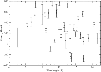
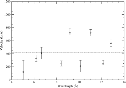
Many of the absorption lines detected by Miller et al. (2005) are much stronger during Period I of our observation (see Table 1). Using only the lines that are detected with a significance above $5\sigma$ , we looked for a systematic red- or blue- shift of the lines, following up on the reported redshift of the lines by Marshall et al. (2001) based on data taken in the low-hard state. The results are summarized in Figure 6 (in the left panel). In this case, although the lines are still systematically redshifted on average, there is not an obvious single-velocity solution. Interestingly, if we limit the results only to those lines that were used by Marshall et al. (2001), as shown in the right panel of Figure 6, we would arrive at an average velocity that is very close to what Marshall et al. reported, although the scatter of data points is much larger in our case. On the other hand, our observation spans binary orbital phases from 0.85 to 0.92, according to the most updated ephemeris (Brocksopp et al. 1999b), while Marshall et al.’s covers a phase range of 0.83–0.86. If the redshift of the lines is related to the focused-wind scenario advocated by Miller et al. (2005), we ought to see a larger (by about 30%) redshift. Given the large uncertainties, as well as the possibility that the wind geometry might be different for different states, it is difficult to draw any definitive conclusions.

Feng et al. (2003) reported the detection of a number of absorption lines of asymmetric profile, when Cyg X-1 was in the high-soft state, which they interpreted as evidence for inflows. The same lines are also present in our data during Period I and are, in fact, much stronger (except for S XVI, as noted in § 3.2). Figure 7 shows an expanded view of the Si and Mg lines, which are the strongest in the group. As is apparent from the figure, the line profile can be fitted fairly well by a Gaussian function in all cases. Therefore, the lines show no apparent asymmetry here. This also seems to be the case for the S and Fe lines, although the statistics of the data are not as good. Taken together, our results and Feng et al.’s imply that that the phenomenon is either unique to the high-soft state (in which Feng et al. made the observation) or is intermittent in nature. We should also note that Feng et al’s observation was carried out around the superior conjunction (i.e., zero orbital phase), where absorption due to the wind is expected to be the strongest (e.g., Wen et al. 1999). It is not clear, however, how such additonal absorption would lead to an asymmetry in the profile of lines.

No emission lines are apparent in our data. Evidence for weak emission lines has been presented (Schulz et al. 2002; Miller et al. 2005) but the significance is marginal in all cases. On the other hand, several absorption edges are easily detected in our data (see Figs. 3 and 4), as first reported and studied in detail by Schulz et al. (2002). The edges can almost certainly be attributed to the interstellar absorption.

We thank Harvey Tananbaum for approving this DDT observation, Norbert Schulz and Herman Marshall for helpful discussion on the pros and cons of various observing configurations, John Houck for help with the use of ISIS and Tim Kallman for help on using XSTAR, and David Huenemoerder for looking into issues related to the Chandra data products. We acknowledge the use of the curve-of-growth analysis script that Taro Kotani has made publicly available. We also thank the anonymous referee for a number of useful comments that led to significant improvement of the manuscript. Support for this work was provided in part by NASA through the Chandra Award DD1-2011X issued by the Chandra X-ray Observatory Center, which is operated by the Smithsonian Astrophysical Observatory for and on behalf of NASA under contract NAS8-03060, and through the LTSA grant NAG5-9998.

References

(1)
(2) Behar, E., & Netzer, H., 2002, ApJ, 570, 165
(3) Blondin, J. M., Stevens, I. R., & Kallman, T. R. 1991, ApJ, 371, 684
(4) Bolton, C. T., 1972, Nature, 235, 271
(5) Brocksopp, C., et al. 1999a, MNRAS, 309, 1063
(6) Brocksopp, C., Tarasov, A. E., Lyuty, V. M., & Roche, P., 1999b, A&A, 343, 861
(7) Cui, W., Heindl, W. A., Rothschild, R. E., Zhang, S. N., Jahoda, K., & Focke, W. 1997a, ApJ, 474, L57
(8) Cui, W., Zhang, S. N., Focke, W., & Swank, J. 1997b, ApJ, 484, 383
(9) Cui, W., Chen, W., & Zhang, S. N. 1997, in 1997 Pacific Rim Conference on Stellar Astrophysics, eds. K. L. Chan, et al., PASP Conf. Ser, vol 138, p. 75
(10) Cui, W., Ebisawa, K., Dotani, T., & Kubota, A. 1998, ApJ, 493, L75
(11) Ebisawa, K., et al. 1996, ApJ, 467, 419
(12) Feng, Y. X., Tennant, A. F., & Zhang, S. N., 2003, ApJ, 597, 1017
(13) Gies, D. R., & Bolton, C. T., 1986, ApJ, 304, 389
(14) Gies, D. R., et al. 2003, ApJ, 583, 424
(15) Houck, J. C., & Denicola, L. A. 2000, in Astronomical Data Analysis Software and Systems IX, eds. N. Manset, C. Veillet, and D. Crabtree, ASP Conf. Proc., Vol. 216, p.591
(16) Kotani, T., Ebisawa, K., Dotani, T., Inoue, H., Nagase, F., Tanaka, Y., & Ueda, Y., 2000, ApJ, 539, 413
(17) LaSala, J., Charles, P. A., Smith, R. A. D., Balucinska-Church, M., & Church, M. J. 1998, MNRAS, 301, 285
(18) Marshall, H. L., Schulz, N. S., Fang, T,. Cui, W., Canizares, C. R., Miller, J. M., & Lewin, W. H. G., 2001, in X-Ray Emmission from Accretion onto Black Holes, eds. T. Yaqoob, & J. H. Krolik, 45 620, 398
(19) McClintock, J. E., & Remillard, R. A. 2006, in Compact Stellar X-ray Sources, Eds. W. H. G. Lewin and M. van der Klis (Cambridge Univ. Press), p157
(20) Miller, J. M., et al. 2005, ApJ, 620, 398
(21) Schulz, N. S., Cui, W., Canizares, C. R., Marshall, H. L., Lee, J. C., Miller, J. M., & Lewin, W. H. G., 2002, ApJ, 565, 1141
(22) Verner, D. A., Verner, E. M. & Ferland, G. J., 1996, At. Data Nucl. Data Tables, 64, 1
(23) Webster, B. L., & Murdin, P., 1972, Nature, 235, 37
(24) Wen, L., Cui, W., Levine, A. M., & Bradt, H. V. 1999, ApJ, 525, 968
(25)

Table 1: Detected Absorption Lines

Ion and Transition	(Å)	(Å)	(km s^-1)	( $10^{-3}$ ph cm^-2s^-1)		(mÅ)	(mÅ)	( $10^{-16}$ cm^-2)	( $10^{-16}$ cm^-2)
	Theoretical	Measured	Shift	Flux(I)	Flux(II)	EW(I)	EW(II)	$N_{z}$ (I)	$N_{z}$ (II)
S XV 1s²-1s2p	5.039^b	5.041(3)	120 $\pm$ 180	1.8(3)	$<$ 0.9	3.8(7)	$<$ 1.5	2.5(5)	$\leq$ 1.0
Si XIV 1s-2p	6.1822^a	6.189(1)	330 $\pm$ 50	3.0(2)	$<$ 0.6	6.9(4)	$<$ 1.0	5.4(3)	$\leq$ 0.7
Si XIII 1s²-1s2p	6.648^b	6.657(2)	410 $\pm$ 90	2.6(2)	$<$ 1.7	6.1(5)	$<$ 2.9	2.4(2)	$\leq$ 1.1
Mg XII 1s-3p	7.1062^a	7.119(3)	540 $\pm$ 130	1.2(2)	$<$ 0.9	2.6(5)	$<$ 1.4	8(2)	$\leq$ 4.0
Al XIII 1s-2p	7.1727^a	$7.191(^{+3}_{-2})$	760 ${}^{+130}_{-80}$	1.3(2)	$<$ 1.7	3.0(5)	$<$ 2.7	1.6(3)^d	$\leq$ 1.5
Fe XXIII 1s²2s2p-1s²2s6d	7.2646^c	7.268(5)	140 $\pm$ 210	1.4(3)	$<$ 2.0	3.1(6)	$<$ 3.3	29(6)	$\leq$ 31
Fe XXIII 1s²2s²-1s²2s5p	7.4722^a	7.480 $(^{+5}_{-4})$	310 ${}^{+200}_{-160}$	0.9(2)	$<$ 1.4	1.9(5)	$<$ 2.3	5(1)	$\leq$ 6.5
Fe XXIV 1s²2s-1s²4p	7.9893^a	8.004(5)	550 $\pm$ 190	2.2(3)	$<$ 1.3	4.7(7)	$<$ 2.2	9(1)	$\leq$ 4.0
Fe XXII 1s²2s²2p-1s²2s²5d	8.0904^c	8.096(3)	210 $\pm$ 110	1.0(2)	$<$ 0.6	2.1(5)	$<$ 1.0	8(2)^d	$\leq$ 3.6
Fe XXII 1s²2s²2p-1s²2s²5d	8.1684^c	8.166(3)	-90 $\pm$ 110	1.0(2)	$<$ 1.1	2.3(5)	$<$ 1.9	9(2)^d	$\leq$ 7.2
Fe XXIII 1s²2s²-1s²2s4p	8.3029^a	8.319(2)	580 $\pm$ 70	3.0(3)	$<$ 0.6	6.6(6)	$<$ 1.0	6.4(6)	$\leq$ 0.9
Mg XII 1s-2p	8.4210^a	8.428(1)	250 $\pm$ 40	5.0(3)	$<$ 0.4	10.8(6)	$<$ 0.7	4.7(3)	$\leq$ 0.3
Fe XXI 1s²2s²2p²-1s²2s²2p5d	8.573^a	8.577(5)	140 $\pm$ 170	1.3(3)	$<$ 0.7	2.8(7)	$<$ 1.2	6(2)	$\leq$ 2.6
Fe XXII 1s²2s²2p-1s²2s2p_1/24p_3/2	8.718^c	8.735 $(^{+2}_{-3})$	580 ${}^{+70}_{-100}$	2.2(3)	$<$ 0.5	4.7 $(^{+7}_{-6})$	$<$ 0.9	7(1)	$\leq$ 1.3
Fe XXI 1s²2s²2p²-1s²2s2p_1/22p_3/24p_3/2	8.8254^c	8.823 $(^{+3}_{-4})$	-80 ${}^{+100}_{-140}$	1.4(3)	$<$ 0.9	3.0 $(^{+7}_{-6})$	$<$ 1.4	21 $(^{+5}_{-4})$	$\leq$ 9.4
Fe XXII 1s²2s²2p-1s²2s²4d	8.98^a	8.978 $(^{+1}_{-2})$	-70 ${}^{+30}_{-70}$	1.8(3)	$<$ 0.9	3.9(6)	$<$ 1.6	4.6(8)^d	$\leq$ 1.8
Fe XXII 1s²2s²2p-1s²2s²4d	9.07^a	9.083 $(^{+2}_{-3})$	430 ${}^{+70}_{-100}$	1.9 $(^{+3}_{-4})$	$<$ 0.6	4.0 $(^{+6}_{-8})$	$<$ 1.0	5.2 ${}^{+0.8}_{-1.1}$	$\leq$ 1.2
Mg XI 1s²-1s2p	9.170^b	9.192 $(^{+2}_{-1})$	720 ${}^{+70}_{-30}$	6.2(4)	$-$	13.5(9)	$-$	2.9(2)	$-$
Fe XXI 1s²2s²2p²-1s²2s²2p4d	9.356^a	9.378(5)	700 $\pm$ 160	1.9(4)	$<$ 2.8	4.3 ${}^{+1.0}_{-0.9}$	$<$ 4.8	9(2)	$\leq$ 10
Fe XXI 1s²2s²2p²-1s²2s²2p4d	9.476^a	9.478(1)	60 $\pm$ 30	3.8(3)	$<$ 0.8	8.6 $(^{+8}_{-7})$	$<$ 1.5	6.6 $(^{+7}_{-6})$ ^d	$\leq$ 1.0
Fe XIX 1s²2s²2p⁴-1s²2s²2p³(²D)5d	9.68^a	9.700(4)	620 $\pm$ 120	4.4 $(^{+5}_{-6})$	$<$ 1.8	9(1)	$<$ 3.1	30(3)	$\leq$ 9.8
Ne X 1s-4p	9.7082^a	9.727 $(^{+2}_{-3})$	580 ${}^{+60}_{-90}$	2.4 $(^{+3}_{-4})$	$<$ 0.7	5.3 $(^{+8}_{-9})$	$<$ 1.2	24(4)	$\leq$ 5.0
Fe XX 1s²2s²2p³-1s²2s²2p²(³P)4d	9.991^a	10.000(1)	270 $\pm$ 30	3.7(4)	$<$ 0.7	8.3(8)	$<$ 1.3	5.6(6)^d	$\leq$ 0.8
Na XI 1s-2p	10.0250^a	10.051(2)	780 $\pm$ 60	5.6 $(^{+5}_{-6})$	$<$ 2.0	13(1)	$<$ 3.5	4.0(3)	$\leq$ 1.0
Fe XX 1s²2s²2p³-1s²2s²2p²(³P)4d	10.12^a	10.127(3)	210 $\pm$ 90	1.7(4)	$<$ 0.3	3.8(9)	$<$ 0.6	2.3(6)^d	$\leq$ 0.4
Ne X 1s-3p	10.2389^a	10.245 $(^{+3}_{-2})$	180 ${}^{+90}_{-60}$	2.7 $(^{+4}_{-5})$	$<$ 0.5	6(1)	$<$ 0.9	9(2)	$\leq$ 1.2
Fe XXIV 1s²2s-1s²3p	10.619^a	10.631 $(^{+2}_{-1})$	340 ${}^{+60}_{-30}$	9.1(6)	$<$ 4.6	22(2)	$<$ 8.9	10(1)	$\leq$ 3.7
Fe XXIV 1s²2s-1s²3p	10.663^a	10.674(3)	310 $\pm$ 80	5.6(6)	$<$ 3.2	14(2)	$<$ 6.2	12(2)	$\leq$ 5.0
Fe XIX 1s²2s²2p⁴-1s²2s²2p³(⁴S)4d	10.816^c	10.818(5)	60 $\pm$ 140	7.0(9)	$<$ 3.0	18(2)	$<$ 6.0	14(2)	$\leq$ 4.3
Fe XXIII 1s²2s²-1s²2s3p	10.981^a	10.990(1)	230 $\pm$ 30	5.5(5)	$<$ 2.7	14(1)	$<$ 5.6	2.4(2)^d	$\leq$ 0.8
Na X 1s²-1s2p	11.0027^a	11.029(2)	720 $\pm$ 50	6.3 $(^{+6}_{-7})$	$<$ 4.4	17(2)	$<$ 9.2	2.7(4)	$\leq$ 1.3
Fe XVIII 1s²2s²2p⁵-1s²2s²2p⁴(¹D)4d	11.326^c	11.33(1)	100 $\pm$ 260	8(1)	$<$ 5.1	23 $(^{+4}_{-3})$	$<$ 11	24 $(^{+4}_{-3})$	$\leq$ 11
Fe XXII 1s²2s²2p-1s²2s2p(³P⁰)3p	11.44^a	11.431(1)	-240 $\pm$ 30	7.3(6)	$<$ 2.5	21(2)	$<$ 5.7	8(1)^d	$\leq$ 1.6
Fe XXII 1s²2s²2p-1s²2s2p(³P⁰)3p	11.51^a	11.500(3)	-260 $\pm$ 80	4.3 $(^{+8}_{-7})$	$<$ 0.6	12(2)	$<$ 1.4	22( ${}^{+5}_{-4}$ )	$\leq$ 2.3
Fe XXII 1s²2s²2p-1s²2s²3d	11.77^a	11.781 $(^{+3}_{-1})$	280 ${}^{+80}_{-30}$	12.6(9)	$<$ 3.8	39(3)	$<$ 9.3	7.5 ${}^{+1.0}_{-0.9}$	$\leq$ 1.2
Fe XXI 1s²2s²2p²-1s²2s2p²3p	11.975^c	11.982(2)	180 $\pm$ 50	9.1(9)	$-$	29(3)	$-$	17( ${}^{+3}_{-2})$	$-$
Ne X 1s-2p	12.1339^a	12.144( ${}^{+2}_{-1}$ )	250 ${}^{+50}_{-20}$	4.7(7)	$<$ 0.06	16(2)	$<$ 0.2	3.9 $(^{+7}_{-6})$ ^d	$\leq$ 0.04
Fe XXI 1s²2s²2p²-1s²2s²2p3d	12.259^a	12.247( ${}^{+3}_{-2}$ )	-290 ${}^{+70}_{-50}$	4.2( ${}^{+8}_{-9}$ )	$<$ 5.4	14(3)	$<$ 14	10(3)^d	$\leq$ 10
Fe XXI 1s²2s²2p²-1s²2s²2p3d	12.285^a	12.304(2)	460 $\pm$ 50	22(1)	$<$ 6.8	75(5)	$<$ 18	12(2)	$\leq$ 1.6
Fe XXI 1s²2s²2p²-1s²2s²2p3d	12.422^c	12.438(2)	390 $\pm$ 50	3.9(8)	$<$ 2.9	14(3)	$<$ 8.1	3.0( ${}^{+9}_{-8})$ ^d	$\leq$ 1.6
Fe XX 1s²2s²2p³-1s²2s2p³3p	12.576^c	12.583( ${}^{+2}_{-3}$ )	170 ${}^{+50}_{-70}$	7(1)	$<$ 3.6	26(4)	$<$ 10	19( ${}^{+6}_{-4}$ )	$\leq$ 5.2
Fe XX 1s²2s²2p³-1s²2s²2p²(³P)3d	12.82^a	12.844(2)	560 $\pm$ 50	26(2)	$<$ 6.5	100(6)	$<$ 20	34 ${}^{+16}_{-10}$	$\leq$ 1.0
Fe XX 1s²2s²2p³-1s²2s²2p_1/22p_3/23d	12.912^c	12.914(3)	50 $\pm$ 70	12(2)	$<$ 4.7	47(6)	$<$ 14	33 ${}^{+11}_{-7}$	$\leq$ 5.9
Fe XX 1s²2s²2p³-1s²2s²2p_1/22p_3/23d	12.965^c	12.953( ${}^{+3}_{-2}$ )	-280 ${}^{+70}_{-50}$	12(1)	$-$	48(6)	$-$	56 ${}^{+25}_{-14}$	$-$
Ne IX 1s²-1s2p	13.448^b	13.448( ${}^{+6}_{-5}$ )	0 ${}^{+130}_{-110}$	9(2)	$<$ 8.5	38(9)	$<$ 30	6( ${}^{+3}_{-2}$ )	$\leq$ 4.1
Fe XIX 1s²2s²2p⁴-1s²2s²2p_1/22p ${}^{2}_{3/2}$ 3d	13.479^c	13.482(3)	70 $\pm$ 70	5(1)	$<$ 3.3	20( ${}^{+6}_{-5}$ )	$<$ 12	1.0( ${}^{+4}_{-3}$ )^d	$\leq$ 0.5
Fe XIX 1s²2s²2p⁴-1s²2s²2p³(²D)3d	13.518^c	13.523(3)	110 $\pm$ 70	16(2)	$-$	70( ${}^{+8}_{-9}$ )	$-$	24 ${}^{+16}_{-9}$	$-$
Fe XVIII 1s²2s²2p⁵-1s²2s²2p⁴(¹D)3d	14.203^a	14.220(3)	360 $\pm$ 40	6(1)	$<$ 4.0	32(7)	$<$ 18	4( ${}^{+3}_{-2}$ )^d	$\leq$ 1.5
Fe XIX 1s²2s²2p⁴-1s²2s²2p³(²P)3s	14.60^a	14.608(5)^e	100 $\pm$ 100	19(3)	20(4)	81 $\pm$ 13	73 $\pm$ 14	200 ${}^{+160}_{-90}$	170 ${}^{+120}_{-60}$
Fe XVIII 1s²2s²2p⁵-1s²2s²2p⁴(³P)3d	14.610^a

Notes. — Results for Periods I and II are both shown for comparison. The errors in parentheses indicate uncertainty in the last digit of the measurement; 1 $\sigma$ errors are shown. Negative flux or EW upper limits (indicating emission) are not shown.
a Verner et al. (1996); b Behar et al. (2002); c ATOMDB 1.3.3; d Unresolved; e The two transitions are equally probable. The average wavelength was used to derive the Doppler-shift of the line.

Refer to caption — Figure 1: Daily-averaged ASM Light Curve of Cyg X-1 during the 2001 state transition. The vertical line indicates the time of the Chandra observation.