Reexamination of spin decoherence in semiconductor quantum dots from equation-of-motion approach

Abstract

The longitudinal and transversal spin decoherence times, $T_{1}$ and $T_{2}$, in semiconductor quantum dots are investigated from equation-of-motion approach for different magnetic fields, quantum dot sizes, and temperatures. Various mechanisms, such as the hyperfine interaction with the surrounding nuclei, the Dresselhaus spin-orbit coupling together with the electron–bulk-phonon interaction, the $g$-factor fluctuations, the direct spin-phonon coupling due to the phonon-induced strain, and the coaction of the electron–bulk/surface-phonon interaction together with the hyperfine interaction are included. The relative contributions from these spin decoherence mechanisms are compared in detail. In our calculation, the spin-orbit coupling is included in each mechanism and is shown to have marked effect in most cases. The equation-of-motion approach is applied in studying both the spin relaxation time $T_{1}$ and the spin dephasing time $T_{2}$, either in Markovian or in non-Markovian limit. When many levels are involved at finite temperature, we demonstrate how to obtain the spin relaxation time from the Fermi Golden rule in the limit of weak spin-orbit coupling. However, at high temperature and/or for large spin-orbit coupling, one has to use the equation-of-motion approach when many levels are involved. Moreover, spin dephasing can be much more efficient than spin relaxation at high temperature, though the two only differs by a factor of two at low temperature.

I Introduction

One of the most important issues in the growing field of spintronics is quantum information processing in quantum dots (QDs) using electron spin.Awschalom ; Hans ; Loss ; Hanson ; Taylor0 A main obstacle is that the electron spin is unavoidably coupled to the environment (such as, the lattice) which leads to considerable spin decoherence (including longitudinal and transversal spin decoherences).Amasha ; Elzerman Various mechanisms, such as, the hyperfine interaction with the surrounding nuclei,Paget ; Meier the Dresselhaus/Rashba spin-orbit coupling (SOC)Dresselhaus ; Yu together with the electron-phonon interaction, $g$-factor fluctuations,Roth the direct spin-phonon coupling due to the phonon-induced strain,Meier and the coaction of the hyperfine interaction and the electron-phonon interaction can lead to the spin decoherence. There are quite a lot of theoretical works on spin decoherence in QD. Specifically, Khaetskii and Nazarov analyzed the spin-flip transition rate using a perturbative approach due to the SOC together with the electron-phonon interaction, $g$-factor fluctuations, the direct spin-phonon coupling due to the phonon-induced strain qualitatively.Khaetskii ; Khaetskii0 ; Nazarov After that, the longitudinal spin decoherence time $T_{1}$ due to the Dresslhaus and/or the Rashba SOC together with the electron-phonon interaction were studied quantitatively in Refs. Woods, ; Sousa, ; Cheng, ; Bulaev, ; Golovach, ; Destefani, ; Jose, ; Falko2, ; Stano, ; Stano2, ; Westfahl, . Among these works, Cheng et al.Cheng developed an exact diagonalization method and showed that due to the strong SOC, the previous perturbation methodKhaetskii0 ; Nazarov ; Woods is inadequate in describing $T_{1}$. Furthermore, they also showed that, the perturbation method previously used missed an important second-order energy correction and would yield qualitatively wrong results if the energy correction is correctly included and only the lowest few states are kept as those in Refs. Khaetskii0, ; Nazarov, ; Woods, . These results were later confirmed by Destefani and Ulloa.Destefani The contribution of the coaction of the hyperfine interaction and the electron-phonon interaction to longitudinal spin decoherence was calculated in Refs. Erlingsson, and Abalmassov, . In contrast to the longitudinal spin decoherence time, there are relatively fewer works on the transversal spin decoherence time, $T_{2}$, also referred to as the spin dephasing time (while the longitudinal spin decoherence time is referred to as the spin relaxation time for short). The spin dephasing time due to the Dresselhaus and/or the Rashba SOC together with the electron-phonon interaction was studied by Semenov and KimSemenov and by Golovach et al..Golovach The contributions of the hyperfine interaction and the $g$-factor fluctuation were studied in Refs. Glazman, ; Khaetskii2, ; Schliemann2, ; Coish, ; Cakir, ; Deng, ; Erlingsson2, ; Shenvi, ; Sousa2, ; Merkulov, ; Pershin, ; Witzel3, ; Yao, ; Witzel2, ; Deng2, and in Ref. Kim, respectively. However, a quantitative calculation of electron spin decoherence induced by the direct spin-phonon coupling due to phonon-induced strain in QDs is still missing. This is one of the issues we are going to present in this paper. In brief, the spin relaxation/dephasing due to various mechanisms has been studied previously in many theoretical works. However, almost all of these works only focus individually on one mechanism. Khaetskii and Nazarov discussed the effects of different mechanisms on the spin relaxation time. Nevertheless, their results are only qualitative and there is no comparison of the relative importance of the different mechanisms.Khaetskii ; Khaetskii0 ; Nazarov Recently, Semenov and Kim discussed various mechanisms contributed to the spin dephasing,Semenov3 where they gave a “phase diagram” to indicate the most important spin dephasing mechanism in Si QD where the SOC is not important. However, the SOC is very important in GaAs QDs. To fully understand the microscopic mechanisms of spin relaxation and dephasing, and to achieve control over the spin coherence in QDs,Witzel ; DeSousa ; JHJiang one needs to gain insight into the relative importance of each mechanism to $T_{1}$ and $T_{2}$ under various conditions. This is one of the main purposes of this paper.

Another issue we are going to address relates to different approaches used in the study of the spin relaxation time. The Fermi-Golden-rule approach, which is widely used in the literature, can be used in calculation of the relaxation time $\tau_{i\to f}$ between any initial state $|i\rangle$ and final state $|f\rangle$.Roth ; Khaetskii ; Khaetskii0 ; Glavin ; Nazarov ; Woods ; Cheng ; Destefani ; lv ; Wang ; Erlingsson ; Abalmassov ; Falko2 ; Sousa ; Bulaev ; Stano ; Stano2 However, the problem is that when the process of the spin relaxation relates to many states, (e.g., when temperature is high, the electron can distribute over many states), one should find a proper way to average over the relaxation times ($\tau_{i\to f}$) of the involved processes to give the total spin relaxation time ($T_{1}$). What makes it difficult in GaAs QDs, is that all the states are impure spin states with different expectation values of spin. In the existing literature, spin relaxation time is given by the average of the relaxation times of processes from the initial state $|i\rangle$ to the final state $|f\rangle$ (with opposite majority spin of $|i\rangle$) weighted by the distribution of the initial states $f_{i}$,Cheng ; lv ; Wang i.e.,

$$T_{1}^{-1}=\sum_{if}f_{i}\tau_{i\to f}^{-1}\ .$$ (1)

This is a good approximation in the limit of small SOC as each state only carries a small amount of minority spin. However, when the SOC is very strong which happens at high levels, it is difficult to find the proper way to perform the average. We will show that Eq. (1) is not adequate any more. Thus, to investigate both $T_{1}$ and $T_{2}$ at finite temperature for arbitrary strength of SOC, we develop an equation-of-motion approach for the many-level system via projection operator techniqueArgyres in the Born approximation. With the rotating wave approximation, we obtain a formal solution to the equation of motion. By assuming a proper initial distribution, we can calculate the evolution of the expectation value of spin. We thus obtain the spin relaxation/dephasing time by the $1/e$ decay of the expectation value of spin operator $\langle S_{z}\rangle$ or $|\langle S_{+}\rangle|$ (to its equilibrium value), with $S_{+}\equiv S_{x}+iS_{y}$. With this approach, we are able to study spin relaxation/dephasing for various temperature, SOC strength, and magnetic field.

For quantum information processing based on electron spin in QDs, the quantum phase coherence is very important. Thus, the spin dephasing time is a more relevant quantity. There are two kinds of spin dephasing times: the ensemble spin dephasing time $T_{2}^{\ast}$ and the irreversible spin dephasing time $T_{2}$. For a direct measurement of an ensemble of QDsBraun or an average over many measurements at different times where the configurations of the environment have been changed,Koppens ; Petta ; Koppens2 it gives the ensemble spin dephasing time $T_{2}^{\ast}$. The irreversible spin dephasing time $T_{2}$ can be obtained by spin echo measurement.Petta ; Koppens2 A widely discussed source which leads to both $T_{2}^{\ast}$ and $T_{2}$ is the hyperfine interaction between the electron spin and the nuclear spins of the lattice. As it has been found that $T_{2}^{\ast}$ is around 10 ns, which is too short and makes a practical quantum information processing difficult in electron spin based qubits in QDs. Thus a spin echo technique is needed to remove the free induction decay and to elongate the spin dephasing time. Fortunately, this technique has been achieved first by Petta et al. for two electron triplet-singlet system and then by Koppens et al. for a single electron spin system. The achieved spin dephasing time is $\sim 1$ $\mu$s, which is much longer than $T_{2}^{\ast}$. We therefore discuss only the irreversible spin dephasing time $T_{2}$ throughout the paper, i.e., we do not consider the free induction decay in the hyperfine-interaction-induced spin dephasing.

It is further noticed that Golovach et al. have shown that the spin dephasing time $T_{2}$ is two times the spin relaxation time $T_{1}$.Golovach However, as temperature increases, this relation does not hold. Semenov and Kim on the other hand reported that the spin dephasing time is much smaller than the spin relaxation time.Semenov In this paper, we calculate the temperature dependence of the ratio of the spin relaxation time to the spin dephasing time and analyze the underlying physics.

This paper is organized as follows: In Sec. II, we present our model and formalism of the equation-of-motion approach. We also briefly introduce all the spin decoherence mechanisms considered in our calculations. In Sec. III we present our numerical results to indicate the contribution of each spin decoherence mechanism to spin relaxation/dephasing time under various conditions based on the equation-of-motion approach. Then we study the problem of how to obtain the spin relaxation time from the Fermi Golden rule when many levels are involved in Sec. IV. The temperature dependence of $T_{1}$ and $T_{2}$ is investigated in Sec. V. We conclude in Sec. VI.

II Model and Formalism

II.1 Model and Hamiltonian

We consider a QD system, where the QD is confined by a parabolic potential $V_{c}(x,y)=\frac{1}{2}m^{\ast}\omega_{0}^{2}(x^{2}+y^{2})$ in the quantum well plane. The width of the quantum well is $a$. The external magnetic field ${\mathbf{B}}$ is along $z$ direction, except in Sec. IV. The total Hamiltonian of the system of electron together with the lattice is:

$$H_{T}=H_{e}+H_{L}+H_{eL}\ ,$$ (2)

where $H_{e}$, $H_{L}$, $H_{eL}$ are the Hamiltonians of the electron, the lattice and their interaction, respectively. The electron Hamiltonian is given by

$$H_{e}=\frac{\mathbf{P}^{2}}{2m^{\ast}}+V_{c}({\mathbf{r}})+H_{Z}+H_{SO}$$ (3)

where $\mathbf{P}=-i\hbar\mathbf{\mbox{\boldmath$\nabla$\unboldmath}}+\frac{e}{c}\bf{A}$ with $\bf{A}=({B_{\perp}}/2)(-y,x)$ ($B_{\perp}$ is the magnetic field along $z$ direction), $H_{Z}=\frac{1}{2}g\mu_{B}{\mathbf{B}}\cdot\mbox{\boldmath$\sigma$\unboldmath}$ is the Zeeman energy with $\mu_{B}$ the Bohr magneton, and $H_{SO}$ is the Hamiltonian of SOC. In GaAs, when the quantum well width is small or the gate-voltage along the growth direction is small, the Rashba SOC is unimportant.flat Therefore, only the Dresselhaus termDresselhaus contributes to $H_{SO}$. When the quantum well width is smaller than the QD radius, the dominant term in the Dresselhaus SOC reads

$$H_{so}=\frac{\gamma_{0}}{\hbar^{3}}\langle P_{z}^{2}\rangle_{{\lambda_{0}}}(-P_{x}\sigma_{x}+P_{y}\sigma_{y})\ ,$$ (4)

with $\gamma_{0}$ denoting the Dresselhaus coefficient, $\lambda_{0}$ being the quantum well subband index of the lowest one and $\langle P_{z}^{2}\rangle_{\lambda}\equiv-\hbar^{2}\int\psi_{z\lambda}^{\ast}(z)\partial^{2}/\partial z^{2}\psi_{z\lambda}(z)dz$. The Hamiltonian of the lattice consists of two parts $H_{L}=H_{ph}+H_{nuclei}$, where $H_{ph}=\sum_{{\mathbf{q}}\eta}\hbar\omega_{{\mathbf{q}}\eta}a^{\dagger}_{{\mathbf{q}}\eta}a_{{\mathbf{q}}\eta}$ ($a^{\dagger}$/$a$ is the phonon creation/annihilation operator) describes the vibration of the lattice and $H_{nuclei}=\sum_{j}\gamma_{I}{\mathbf{B}}\cdot{\mathbf{I}}_{j}$ ($\gamma_{I}$ is the gyro-magnetic ratios of the nuclei and ${\mathbf{I}}_{j}$ is the spin of the $j$-th nucleus) describes the precession of the nuclear spins of the lattice in the external magnetic field. We focus on the spin dynamics due to hyperfine interaction at a time scale much smaller than the nuclear dipole-dipole correlation time ($10^{-4}$ s in GaAsMerkulov ; Coish ), where the nuclear dipole-dipole interaction can be ignored. Under this approximation, the equation of motion for the reduced electron system can be obtained which only depends on the initial distribution of the nuclear spin bath.Coish The interaction between the electron and the lattice also has two parts $H_{eL}=H_{eI}+H_{e-ph}$, where $H_{eI}$ is the hyperfine interaction between the electron and nuclei and $H_{e-ph}$ represents the electron-phonon interaction which is further composed of the electron–bulk-phonon (BP) interaction $H_{ep}$, the direct spin-phonon coupling due to the phonon-induced strain $H_{strain}$ and phonon-induced $g$-factor fluctuation $H_{g}$.

II.2 Equation-of-motion approach

The equations of motion can describe both the coherent and the dissipative dynamics of the electron system. When the quasi-particles of the bath relax much faster than the electron system, the Markovian approximation can be made; otherwise the kinetics is the non-Markovian. For electron-phonon coupling, due to the fast relaxation of the phonon bath and the weak electron-phonon scattering, the kinetics of the electron is Markovian. Nevertheless, as the nuclear spin bath relaxes much slower than the electron spin, the kinetics due to the coupling with nuclei is of non-Markovian type.Glazman ; Schliemann2 ; Coish It is further noted that there is also a contribution from the coaction of the electron-phonon and electron-nuclei couplings, which is a fourth order coupling to the bath. For this contribution, the decoherence of spin is mainly controlled by the electron-phonon scattering while the hyperfine (Overhauser) fieldSlichter acts as a static magnetic field. Thus, this fourth order coupling is also Markovian. Finally, since the electron orbit relaxation is much faster than the electron spin relaxation,Fujisawa we always assume a thermo-equilibrium initial distribution of the orbital degrees of freedom.

Generally, the interaction between the electron and the quasi-particle of the bath is weak. Therefore the first Born approximation is adequate in the treatment of the interaction. Under this approximation, the equation of motion for the electron system coupled to the lattice environment can be obtained with the help of the projection operator technique.Argyres We then assume a sudden approximation so that the initial distribution of the whole system is $\rho(t=0)=\rho^{e}(0)\otimes\rho^{L}(0)$, where $\rho^{e}$, $\rho^{L}$ is the density matrix of the system and bath respectively. This approximation corresponds to a sudden injection of the electron into the quantum dot, which is reasonable for genuine experimental setup.Coish As the initial distribution of the the lattice $\rho^{L}(0)$ commutates with the Hamiltonian of the lattice $H_{L}$, the equation of motion can be written as

$$\frac{d\rho^{e}(t)}{dt}=-\frac{i}{\hbar}[H_{e}+\mbox{Tr}_{L}(H_{eL}\rho^{L}(0)),\rho^{e}(t)]$$

$$\hskip 17.07182pt\mbox{}-\frac{1}{\hbar^{2}}\int_{0}^{t}d\tau\mbox{Tr}_{L}[H_{eL},U_{0}(\tau)(\hat{\cal{P}}[H_{eL},\rho^{e}(t-\tau)$$

$$\hskip 71.13188pt\otimes\rho^{L}(0)])U_{0}^{\dagger}(\tau)]\ ,$$ (5)

where $\rho^{e}(t)$ is the density operator of the electron system at time $t$, $\mbox{Tr}_{L}$ stands for the trace over the lattice degree of freedom, and $U_{0}(\tau)=e^{-i(H_{L}+H_{e})\tau}$ is time-evolution operator without $H_{eL}$. $\hat{\cal{P}}=\hat{1}-\rho^{L}(0)\otimes\mbox{Tr}_{L}$ is the projection operator. The initial distribution of the phonon system is chosen to be the thermo-equilibrium distribution.Golovach It has been shown by previous theoretical studies that the initial state of the nuclear spin bath is crucial to the spin dephasing and relaxation.Glazman ; Schliemann2 ; Coish Although it may take a long time (e.g., seconds) for the nuclear spin system to relax to its thermo-equilibrium state, one can still assume that its initial state is the thermo-equilibrium one. This assumption corresponds to the genuine case of enough long waiting time during every individual measurement. For a typical setup at above 10 mK and with about 10 T external magnetic field, the thermo-equilibrium distribution is a distribution with equal probability on every state. For these initial distributions of phonons and nuclear spins, the term $\mbox{Tr}_{L}(H_{eL}\rho^{L}(0))$ is zero. Thus,

$$\hat{\cal{P}}[H_{eL},\rho^{e}(t-\tau)\otimes\rho^{L}(0)]=[H_{eL},\rho^{e}(t-\tau)\otimes\rho^{L}(0)]\ .$$ (6)

The equation of motion is then simplified to,

$$\frac{d\rho^{e}(t)}{dt}=-\frac{i}{\hbar}[H_{e},\rho^{e}(t)]-\frac{1}{\hbar^{2}}\int_{0}^{t}d\tau\mbox{Tr}_{L}[H_{eL},[H^{I}_{eL}(-\tau),$$

$$U^{e}_{0}(t)\rho^{Ie}(t-\tau){U^{e}_{0}}^{\dagger}(t)\rho^{L}(0)]]\ ,$$ (7)

where $H^{I}_{eL}$ and $\rho^{Ie}$ are the corresponding operators ($H_{eL}$ and $\rho^{e}$ ) in the interaction picture, and $U^{e}_{0}(t)=e^{-iH_{e}t}$ is the time-evolution operator of $H_{e}$. It should be further noted that the first Born approximation can not fully account for the non-Markovian dynamics due to the hyperfine interaction with nuclear spins.Fulton ; Coish Only when the Zeeman splitting is much larger than the fluctuating Overhauser shift, the first Born approximation is adequate. For GaAs QDs, this requires $B\gg 3.5$ T.Coish In this paper, we focus on the study of spin dephasing for the high magnetic field regime of $B>3.5$ T under the first Born approximation, where the second Born approximation only affects the long-time behavior.Coish Later we will argue that this correction of long time dynamics changes the spin dephasing time very little.

II.2.1 Markovian kinetics

The kinetics due to the coupling with phonons can be investigated within the Markovian approximation, where the equation of motion reduces to,

$$\frac{d\rho^{e}(t)}{dt}=-\frac{i}{\hbar}[H_{e},\rho^{e}(t)]-\frac{1}{\hbar^{2}}\int_{0}^{t}d\tau\mbox{Tr}_{ph}[H_{e-ph},$$

$$\hskip 28.45274pt\mbox{}[H^{I}_{e-ph}(-\tau),\rho^{e}(t)\otimes\rho^{ph}(0)]]\ .$$ (8)

Here $\mbox{Tr}_{ph}$ is the trace over phonon degrees of freedom and $\rho^{ph}(0)$ is the initial distribution of the phonon bath. Within the basis of the eigen-states of the electron Hamiltonian, $\{|\ell\rangle\}$, the above equation reads,

$$\frac{d}{dt}\rho_{\ell_{1}\ell_{2}}^{e} =-i\frac{(\varepsilon_{\ell_{1}}-\varepsilon_{\ell_{2}})}{\hbar}\rho_{\ell_{1}\ell_{2}}^{e}$$ (9)

$$-\Big{\{}\frac{1}{\hbar^{2}}\int_{0}^{t}\!\!d{\tau}\sum_{\ell_{3}\ell_{4}}\mbox{Tr}_{p}(H_{\ell_{1}\ell_{3}}^{e-ph}H_{\ell_{3}\ell_{4}}^{I\ e-ph}\rho_{\ell_{4}\ell_{2}}^{e}\otimes\rho_{eq}^{p}$$

$$\hskip 14.22636pt-H_{\ell_{1}\ell_{3}}^{I\ e-ph}\rho_{\ell_{3}\ell_{4}}^{e}\otimes\rho_{eq}^{p}H_{\ell_{4}\ell_{2}}^{e-ph})+H.c.\Big{\}}\ .$$

Here $H_{\ell_{1}\ell_{3}}^{e-ph}=\langle\ell_{1}|H_{e-ph}|\ell_{3}\rangle$ and $H_{\ell_{1}\ell_{3}}^{I\ e-ph}=\langle\ell_{1}|H^{I}_{e-ph}(-\tau)|\ell_{3}\rangle$. A general form of the electron-phonon interaction reads

$$H_{e-ph}=\sum_{{\bf q}\eta}\Phi_{{\bf q}\eta}(a_{{\bf q}\eta}+a^{\dagger}_{-{\bf q}\eta})X_{{\bf q}\eta}({\bf r},{\mbox{\boldmath$\sigma$\unboldmath}})\ .$$ (10)

Here, $\eta$ represents the phonon branch index; $\Phi_{{\bf q}\eta}$ is the matrix element of the electron-phonon interaction; $a_{{\bf q}\eta}$ is the phonon annihilation operator; $X_{{\bf q}\eta}({\bf r},{\mbox{\boldmath$\sigma$\unboldmath}})$ denotes a function of electron position and spin. Substituting this into Eq. (9), we obtain, after integration within the Markovian approximation,JHJiang

$$\frac{d}{dt}\rho_{\ell_{1}\ell_{2}}^{e} = i\frac{(\varepsilon_{\ell_{1}}-\varepsilon_{\ell_{2}})}{\hbar}\rho_{\ell_{1}\ell_{2}}^{e}$$ (11)

$$-\Big{\{}\frac{\pi}{\hbar^{2}}\sum_{\ell_{3}\ell_{4}}\sum_{{\bf q}\eta}|\Phi_{{\bf q}\eta}|^{2}\{X_{\ell_{1}\ell_{3}}^{{\bf q}\eta}X_{\ell_{4}\ell_{3}}^{{\bf q}\eta\ast}\rho_{\ell_{4}\ell_{2}}^{e}$$

$$\hskip 14.22636pt\times C_{{\bf q}\eta}(\varepsilon_{\ell_{4}}-\varepsilon_{\ell_{3}})\mbox{}-X_{\ell_{4}\ell_{2}}^{{\bf q}\eta}X_{\ell_{3}\ell_{1}}^{{\bf q}\eta\ast}\rho_{\ell_{3}\ell_{4}}^{e}$$

$$\hskip 14.22636pt\times C_{{\bf q}\eta}(\varepsilon_{\ell_{3}}-\varepsilon_{\ell_{1}})\}+H.c.\ \Big{\}}$$

in which $X_{\ell_{1}\ell_{2}}^{{\bf q}\eta}=\langle\ell_{1}|X_{{\bf q}\eta}({\bf r},{\mbox{\boldmath$\sigma$\unboldmath}})|\ell_{2}\rangle$, and $C_{{\bf q}\eta}(\Delta\varepsilon)=\bar{n}(\omega_{{\bf q}\eta})\delta(\Delta\varepsilon+\omega_{{\bf q}\eta})+[\bar{n}(\omega_{{\bf q}\eta})+1]\delta(\Delta\varepsilon-\omega_{{\bf q}\eta})$. Here $\bar{n}(\omega_{{\bf q}\eta})$ represents the Bose distribution function. Equation (11) can be written in a more compact form

$$\frac{d}{dt}\rho_{\ell_{1}\ell_{2}}^{e}=-\sum_{\ell_{3}\ell_{4}}\Lambda_{\ell_{1}\ell_{2}\ell_{3}\ell_{4}}\rho_{\ell_{3}\ell_{4}}^{e}\ ,$$ (12)

which is a linear differential equation. This equation can be solved by diagonalizing ${\bf\Lambda}$. Given an initial distribution $\rho_{\ell_{1}\ell_{2}}^{e}(0)$, the density matrix $\rho_{\ell_{1}\ell_{2}}^{e}(t)$ and the expectation value of any physical quantity $\langle O\rangle_{t}=\mbox{Tr}({\hat{O}}{\bf{\rho}}^{e}(t))$ at time $t$ can be obtained:JHJiang

$$\langle O\rangle_{t} = \mbox{Tr}({\hat{O}}{\bf{\rho}}^{e})$$ (13)

$$= \sum_{\ell_{1}\cdots\ell_{6}}\langle\ell_{2}|{\hat{O}}|\ell_{1}\rangle{\bf P}_{(\ell_{1}\ell_{2})(\ell_{3}\ell_{4})}$$

$$\mbox{}\times e^{-{\bf\Gamma}_{(\ell_{3}\ell_{4})}t}{\bf P}_{(\ell_{3}\ell_{4})(\ell_{5}\ell_{6})}^{-1}\rho_{\ell_{5}\ell_{6}}^{e}(0)$$

with ${\bf\Gamma}={\bf P}^{-1}{\bf\Lambda}{\bf P}$ being the diagonal matrix and ${\bf P}$ representing the transformation matrix. To study spin dynamics, we calculate $\langle S_{z}\rangle_{t}$ ($|\langle S_{+}\rangle_{t}|$) and define the spin relaxation (dephasing) time as the time when $\langle S_{z}\rangle_{t}$ ($|\langle S_{+}\rangle_{t}|$) decays to $1/e$ of its initial value (to its equilibrium value).

II.2.2 Non-Markovian kinetics

Experiments have already shown that for a large ensemble of quantum dots or for an ensemble of many measurements on the same quantum dot at different times, the spin dephasing time due to hyperfine interaction is quite short, $\sim 10$ ns.Braun ; Koppens ; Petta ; Koppens2 This rapid spin dephasing is caused by the ensemble broadening of the precession frequency due to the hyperfine fields.Merkulov When the external magnetic field is much larger than the random Overhauser field, the rotation due to the Overhauser field perpendicular to the magnetic field is blocked. Only the broadening of the Overhauser field parallel to the magnetic field contribute to the spin dephasing. To describe this free induction decay for this high magnetic field case, we write the hyperfine interaction into two parts: $H_{eI}={\mathbf{h}}\cdot{\mathbf{S}}=H_{eI1}+H_{eI2}$. Here ${\mathbf{h}}=(h_{x},h_{y},h_{z})$ and ${\mathbf{S}}=(S_{x},S_{y},S_{z})$ are the Overhauser field and the electron spin respectively. $H_{eI1}=h_{z}S_{z}$ and $H_{eI2}=\frac{1}{2}(h_{+}S_{-}+h_{-}S_{+})$ with $h_{\pm}=h_{x}\pm ih_{y}$. The longitudinal part $H_{eI1}$ is responsible for the free induction decay, while the transversal part $H_{eI2}$ is responsible for high order irreversible decay. As the rapid free induction decay can be removed by spin echo,Petta ; Koppens2 elongating the spin dephasing time to $\sim 1$ $\mu$s which is more favorable for quantum computation and quantum information processing, we then discuss only the irreversible decay. We first classify the states of the nuclear spin system with its polarization. Then we reconstruct the states within the same class to make it spatially uniform. These uniformly polarized pure states, $|n\rangle$’s, are eigen-states of $h_{z}$. They also form a complete-orthogonal basis of the nuclear spin system. A formal expression of $|n\rangle$ isCoish

$$|n\rangle=\sum_{m_{1}\cdots m_{N}}\alpha^{n}_{m_{1}\cdots m_{N}}\bigotimes_{j=1}^{N}|I,m_{j}\rangle\ .$$ (14)

Here $|I,m_{j}\rangle$ denotes the eigen-state of the $z$-component of the $j$-th nuclear spin $I_{jz}$ with the eigenvalue $\hbar m_{j}$. $N$ denotes the number of the nuclei. The equation of motion for the case with initial nuclear spin state $\rho^{ns}_{1}(0)=|n\rangle\langle n|$ is given byCoish

$$\frac{d\rho^{e}(t)}{dt} = -\frac{i}{\hbar}[H_{e}+\mbox{Tr}_{ns}(H_{eI}\rho^{ns}_{1}(0)),\rho^{e}(t)]$$ (15)

$$\mbox{}-\frac{1}{\hbar^{2}}\int_{0}^{t}d\tau\mbox{Tr}_{ns}[H_{eI2},U^{eI}_{0}(\tau)$$

$$\times[H_{eI2},\rho^{e}(t-\tau)\otimes\rho^{ns}_{1}(0)]{U^{eI}_{0}}^{\dagger}(\tau)]\ .$$

As in traditional projection operator technique, the dynamics of the nuclear spin subsystem is incorporated self-consistently in the last term.Coish ; Argyres Here $\mbox{Tr}_{ns}$ is the trace over nuclear spin degrees of freedom. $U^{eI}_{0}(\tau)=\exp[-i\tau(H_{e}+H_{I}+H_{eI1})]$. The Overhauser field is given by ${\mathbf{h}}=\sum_{j}Av_{0}{\mathbf{I}}_{j}\delta({\mathbf{r}}-{\mathbf{R}}_{j})$, where the constants $A$ and $v_{0}$ are given later. ${\mathbf{I}}_{j}$ and ${\mathbf{R}}_{j}$ are the spin and position of $j$-th nucleus respectively. As mentioned above, the initial state of the nuclear spin bath is chosen to be a state with equal probability of each state, therefore $\rho^{ns}(0)=\sum_{n}1/N_{w}|n\rangle\langle n|$, with $N_{w}=\sum_{n}1$ being the number of states of the basis $\{|n\rangle\}$. To quantify the irreversible decay, we calculate the time evolution of $S_{+}^{(n)}$ for every case with initial nuclear spin state $|n\rangle$. We then sum over $n$ and obtain

$$||\langle S_{+}\rangle_{t}||=\sum_{n}|\langle S_{+}^{(n)}\rangle_{t}|.$$ (16)

It is noted that the summation is performed after the absolute value of $\langle S_{+}^{(n)}\rangle_{t}$. Therefore, the destructive interference due to the difference in precession frequency $\omega_{zn}$, which originates from the longitudinal part of the hyperfine interaction ($H_{eI1}$), is removed. We thus use $1/e$ decay of the envelope of $||\langle S_{+}\rangle_{t}||$ to describe the irreversible spin dephasing time $T_{2}$. Similar description has been used in the irreversible spin dephasing in semiconductor quantum wellsWu and the irreversible inter-band optical dephasing in semiconductors.Fossi ; Shah

Expanding Eq. (15) in the basis of $\{|n\rangle\}$, one obtains,

$$\frac{d}{dt}\rho_{\ell_{1}\ell_{2}}^{e} =-\frac{i}{\hbar}\sum_{\ell_{3}}\Big{\{}(\varepsilon_{\ell_{1}}\delta_{\ell_{1}\ell_{3}}+H_{n\ell_{1};n\ell_{3}}^{eI1})\rho^{e}_{\ell_{3}\ell_{2}}$$ (17)

$$\hskip 17.07182pt-\rho^{e}_{\ell_{1}\ell_{3}}(\varepsilon_{\ell_{3}}\delta_{\ell_{3}\ell_{2}}+H_{n\ell_{3};n\ell_{2}}^{eI1})\Big{\}}$$

$$-\Big{\{}\frac{1}{\hbar^{2}}\int_{0}^{t}\!\!d{\tau}\sum_{n_{1}}\sum_{\ell_{3}\ell_{4}}[H_{n\ell_{1};n_{1}\ell_{3}}^{eI2}H_{n_{1}\ell_{3};n\ell_{4}}^{I\ eI2}\rho_{\ell_{4}\ell_{2}}^{e}(t-\tau)$$

$$-H_{n\ell_{1};n_{1}\ell_{3}}^{I\ eI2}\rho_{\ell_{3}\ell_{4}}^{e}(t-\tau)H_{n_{1}\ell_{4};n\ell_{2}}^{eI2}]+H.c.\Big{\}}\ .$$

Here $H_{n\ell_{1};n_{1}\ell_{3}}^{eI2}=\langle n\ell_{1}|H_{eI2}|n_{1}\ell_{3}\rangle$ and $H_{n\ell_{1};n_{1}\ell_{3}}^{I\ eI2}=\langle n\ell_{1}|H^{I}_{eI2}(-\tau)|n_{1}\ell_{3}\rangle$. For simplicity, we neglect the terms concerning different orbital wavefunctions which are much smaller. For small spin mixing, assuming an equilibrium distribution in orbital degree of freedom, under rotating wave approximation, and trace over the orbital degree of freedom, we finally arrive at

$$\frac{d}{dt}\langle S_{+}^{(n)}\rangle_{t} = i\omega_{zn}\langle S_{+}^{(n)}\rangle_{t}-\frac{1}{\hbar^{2}}\int^{t}_{0}d\tau\{\frac{1}{4}\sum_{kn^{\prime}}f_{k}([h_{+}]_{k{n}{n^{\prime}}}$$ (18)

$$\mbox{}\times[h_{-}]_{{kn^{\prime}}{n}}+[h_{-}]_{k{n}{n^{\prime}}}[h_{+}]_{{kn^{\prime}}{n}})$$

$$\mbox{}\times\exp[i\tau(\omega_{kn}-\omega_{kn^{\prime}})]\}\langle S_{+}^{(n)}\rangle_{t-\tau}\ .$$

Here $\omega_{zn}=\sum_{k}f_{k}(E_{zk}/\hbar+\omega_{kn})$ with $E_{zk}$ representing the electron Zeeman splitting of the $k$-th orbital level. $[h_{i}]_{knn^{\prime}}=\langle n|\langle k|h_{i}|k\rangle|n^{\prime}\rangle$ ($i=\pm,z$). $\omega_{kn}=[h_{z}]_{knn}+\epsilon_{nz}$ with $\epsilon_{nz}$ denoting the nuclear Zeeman splitting which is very small and can be neglected. By solving the above equation, we obtain $|\langle S_{+}^{(n)}\rangle_{t}|$ for a given $|n\rangle$. We then sum over $n$ and determine the irreversible spin dephasing time $T_{2}$ as $1/e$ decay of the envelop of $||\langle S_{+}\rangle_{t}||$. By noting that only the polarization of nuclear spin state $|n\rangle$ determines the evolution of $|\langle S_{+}^{(n)}\rangle_{t}|$, the summation over $n$ is then reduced to summation over polarization which becomes a integration for large $N$. This integration can be handled numerically.

In the limiting case of zero SOC and very low temperature, only the lowest two Zeeman sublevels are concerned. The equation for $\langle S_{+}\rangle_{t}$ with initial nuclear spin state $\rho^{ns}_{1}(0)=|n\rangle\langle n|$ reduce to

$$\frac{d}{dt}\langle S_{+}\rangle_{t}=i\omega_{zn}\langle S_{+}\rangle_{t}-\frac{1}{\hbar^{2}}\int^{t}_{0}d\tau\{\frac{1}{4}\sum_{n^{\prime}}([h_{+}]_{{n}{n^{\prime}}}$$ (19)

$$\mbox{}\times[h_{-}]_{{n^{\prime}}{n}}+[h_{-}]_{{n}{n^{\prime}}}[h_{+}]_{{n^{\prime}}{n}})\exp[i\tau(\omega_{n}-\omega_{n^{\prime}})]\}\langle S_{+}\rangle_{t-\tau}$$

$$= i\omega_{z}\langle S_{+}\rangle_{t}-\int^{t}_{0}d\tau\Sigma(\tau)\langle S_{+}\rangle_{t-\tau}\ .$$

In this equation $\omega_{zn}=(g\mu_{B}B+[h_{z}]_{nn^{\prime}})/\hbar$, $[h_{\xi}]_{nn^{\prime}}=\langle n|\langle\psi_{1}|h_{\xi}|\psi_{1}\rangle|n^{\prime}\rangle$ ($\xi=\pm,z$ and $\psi_{1}$ is the orbital quantum number of the ground state), and $\omega_{n}=[h_{z}]_{nn}$. Similar equation has been obtained by Coish and Loss,Coish and later by Deng and HuDeng at very low temperature such that only the lowest two Zeeman sublevels are considered. Coish and Loss also presented an efficient way to evaluate $\Sigma(\tau)$ in terms of their Laplace transformations, $\Sigma(s)=\int_{0}^{\infty}d\tau e^{-s\tau}\Sigma(\tau)$. They gave,

$$\Sigma(s) = \frac{1}{4\hbar^{2}}\sum_{n^{\prime}}([h_{+}]_{{n}{n^{\prime}}}[h_{-}]_{{n^{\prime}}{n}}$$ (20)

$$\mbox{}+[h_{-}]_{{n}{n^{\prime}}}[h_{+}]_{{n^{\prime}}{n}})/(s-i\delta\omega_{nn^{\prime}})\ ,$$

with $\delta\omega_{nn^{\prime}}=\frac{1}{2}(\omega_{n}-\omega_{n^{\prime}})$. With the help of this technique, we are able to investigate the spin dephasing due to the hyperfine interaction.

II.3 Spin decoherence mechanisms

In this subsection we briefly summarize all the spin decoherence mechanisms. It is noted that the SOC modifies all the mechanisms. This is because the SOC modifies the Zeeman splittingCheng and the spin-resolved eigen-states of the electron Hamiltonian, it hence greatly changes the effect of the electron-BP scattering.Cheng These two modifications, especially the modification of the Zeeman splitting, also change the effect of other mechanisms, such as, the direct spin-phonon coupling due to the phonon-induced strain, the $g$-factor fluctuation, the coaction of the electron-phonon interaction and the hyperfine interaction. In the literature, except for the electron-BP scattering, the effects from the SOC are neglected except for the work by Woods et al.Woods in which the spin relaxation time between the two Zeeman sub-levels of the lowest electronic state due to the phonon-induced strain is investigated. However, the perturbation method they used does not include the important second-order energy correction. In our investigation, the effects of the SOC are included in all the mechanisms and we will show that they lead to marked effects in most cases.

II.3.1 SOC together with electron-phonon scattering

As the SOC mixes different spins, the electron-BP scattering can induce spin relaxation and dephasing. The electron-BP coupling is given by

$$H_{ep}=\sum_{{\mathbf{q}}\eta}M_{{\mathbf{q}}\eta}(a_{{\mathbf{q}}\eta}+a^{\dagger}_{-{\mathbf{q}}\eta})e^{i{\mathbf{q}}\cdot{\mathbf{r}}}\ ,$$ (21)

where $M_{{\mathbf{q}}\eta}$ is the matrix element of the electron-phonon interaction. In the general form of the electron phonon interaction $H_{e-ph}$, $\Phi_{{\bf q}\eta}=M_{{\mathbf{q}}\eta}$ and $X_{{\bf q}\eta}({\bf r},{\mbox{\boldmath$\sigma$\unboldmath}})=e^{i{\mathbf{q}}\cdot{\mathbf{r}}}$. $|M_{{\mathbf{q}}sl}|^{2}=\hbar\Xi^{2}q/2\rho v_{sl}V$ for the electron-BP coupling due to the deformation potential. For the piezoelectric coupling, $|M_{{\mathbf{q}}pl}|^{2}=(32\hbar\pi^{2}e^{2}e_{14}^{2}/\kappa^{2}\rho v_{sl}V)[(3q_{x}q_{y}q_{z})^{2}/q^{7}]$ for the longitudinal phonon mode and $\sum_{j=1,2}|M_{{\mathbf{q}}pt_{j}}|^{2}=[32\hbar\pi^{2}e^{2}e_{14}^{2}/(\kappa^{2}\rho v_{st}q^{5}V)][q_{x}^{2}q_{y}^{2}+q_{y}^{2}q_{z}^{2}+q_{z}^{2}q_{x}^{2}-(3q_{x}q_{y}q_{z})^{2}/q^{2}]$ for the two transverse modes. Here $\Xi$ stands for the acoustic deformation potential; $\rho$ is the GaAs volume density; $V$ is the volume of the lattice; $e_{14}$ is the piezoelectric constant and $\kappa$ denotes the static dielectric constant. The acoustic phonon spectra $\omega_{{\mathbf{q}}ql}=v_{sl}q$ for the longitudinal mode and $\omega_{{\mathbf{q}}pt}=v_{st}q$ for the transverse mode with $v_{sl}$ and $v_{st}$ representing the corresponding sound velocities.

Besides the electron-BP scattering, electron also couples to vibrations of the confining potential, i.e., the surface-phonons,Abalmassov

$$\delta V({\mathbf{r}})=-\sum_{{\bf q}\eta}\sqrt{\frac{\hbar}{2\rho\omega_{{\bf q}\eta}V}}(a_{{\bf q}\eta}+a_{-{\bf q}\eta}^{\dagger})\mbox{\boldmath$\epsilon$\unboldmath}_{{\bf q}\eta}\cdot{\mathbf{\nabla}}_{{\bf r}}V_{c}({\bf r})\ ,$$ (22)

in which $\epsilon$_qη is the polarization vector of a phonon mode with wave-vector ${\mathbf{q}}$ in branch $\eta$. However, this contribution is much smaller than the electron-BP coupling. Compared to the coupling due to the deformation potential for example, the ratio of the two coupling strengths is $\approx\hbar\omega_{0}/\Xi ql_{0}$ , where $l_{0}$ is the characteristic length of the quantum dot and $\hbar\omega_{0}$ is the orbital level splitting. The phonon wave-vector $q$ is determined by the energy difference between the final and initial states of the transition. Typically phonon transitions between Zeeman sublevels and different orbital levels, $ql_{0}$ ranges from $0.1$ to $10$. Bearing in mind that $\hbar\omega_{0}$ is about 1 meV while $\Xi=7$ eV in GaAs, $\hbar\omega_{0}/\Xi ql_{0}$ is about $10^{-3}$. The piezoelectric coupling is of the same order as the deformation potential. Therefore spin decoherence due to the electron–surface-phonon coupling is negligible.

II.3.2 Direct spin-phonon coupling due to phonon-induced strain

The direct spin-phonon coupling due to the phonon-induced strain is given byDyakonov

$$H_{strain}=\frac{1}{2}{\mathbf{h}}^{s}(\mathbf{p})\cdot{\mbox{\boldmath$\sigma$\unboldmath}}\ ,$$ (23)

where $h_{x}^{s}=-Dp_{x}({\epsilon}_{yy}-{\epsilon}_{zz})$, $h_{y}^{s}=-Dp_{y}({\epsilon}_{zz}-{\epsilon}_{xx})$ and $h_{z}^{s}=-Dp_{z}({\epsilon}_{xx}-{\epsilon}_{yy})$ with $\mathbf{p}=(p_{x},p_{y},p_{z})=-i\hbar{\mbox{\boldmath$\nabla$\unboldmath}}$  and $D$ being the material strain constant. ${\epsilon}_{ij}$ ($i,j=x,y,z$) can be expressed by the phonon creation and annihilation operators:

$${\epsilon}_{ij}=\sum_{{\mathbf{q}}\eta=l,t_{1},t_{2}}\frac{i}{2}\sqrt{\frac{\hbar}{2\rho{\omega_{{\mathbf{q}}\eta}V}}}(a_{{\mathbf{q}},\eta}+a_{-{\mathbf{q}},\eta}^{+})(\xi_{i\eta}q_{j}$$ (24)

$$\mbox{}+\xi_{j\eta}q_{i})e^{i{\mathbf{q}}\cdot{\mathbf{r}}}\ ,$$

in which $\xi_{il}=q_{i}/q$ for the longitudinal phonon mode and $(\xi_{xt_{1}},\xi_{yt_{1}},\xi_{zt_{1}})=(q_{x}q_{z},q_{y}q_{z},-q_{\|}^{2})/qq_{\|}$, $(\xi_{xt_{2}},\xi_{yt_{2}},\xi_{zt_{2}})=(q_{y},-q_{x},0)/q_{\|}$ for the two transverse phonon modes with $q_{\|}=\sqrt{q_{x}^{2}+q_{y}^{2}}$. Therefore, in the general form of electron-phonon interaction $H_{e-ph}$, $\Phi_{{\mathbf{q}}\eta}=-iD\sqrt{\hbar/(32\rho\omega_{{\mathbf{q}}\eta}V)}$ and $X_{{\mathbf{q}}\eta}({\mathbf{r}},{\mbox{\boldmath$\sigma$\unboldmath}})=\sum_{ijk}\epsilon_{ijk}(\xi_{j\eta}q_{j}-\xi_{k\eta}q_{k})p_{i}e^{i{\mathbf{q}}\cdot{\mathbf{r}}}\sigma_{i}$ with $\epsilon_{ijk}$ denoting the Levi-Civita tensor.

II.3.3 $g$-factor fluctuation

The spin-lattice interaction via phonon modulation of the $g$-factor is given byRoth

$$H_{g}=\frac{\hbar}{2}\sum_{ijkl=x,y,z}A_{ijkl}\mu_{B}B_{i}\sigma_{j}{\epsilon}_{kl}\ ,$$ (25)

where ${\epsilon}_{kl}$ is given in Eq. (24) and $A_{ijkl}$ is a tensor determined by the material. Therefore in $H_{e-ph}$, $\Phi_{{\bf q}\eta}=i\sqrt{\hbar/(32\rho\omega_{{\mathbf{q}}\eta}V)}$ and $X_{{\bf q}\eta}({\mathbf{r}},{\mbox{\boldmath$\sigma$\unboldmath}})=\sum_{i,j,k,l}A_{i,j,k,l}\mu_{B}B_{i}(\xi_{k\eta}q_{k}-\xi_{l\eta}q_{l})\sigma_{j}e^{i{\mathbf{q}}\cdot{\mathbf{r}}}$. Due to the axial symmetry with respect to the $z$-axis, and keeping in mind that the external magnetic field is along the $z$ direction, the only finite element of $H_{g}$ is $H_{g}=[(A_{33}-A_{31}){\epsilon}_{zz}+A_{31}\sum_{i}{\epsilon}_{ii}]\hbar{\mu_{B}B}\sigma_{z}/2$ with $A_{33}=A_{zzzz}$, $A_{31}=A_{zzxx}$ and $A_{66}=A_{xyxy}$. $A_{33}+2A_{31}=0$.Kim

II.3.4 Hyperfine interaction

The hyperfine interaction between the electron and nuclear spins isAbragam

$$H_{eI}({\mathbf{r}})=\sum_{j}Av_{0}{\mathbf{S}}\cdot{\mathbf{I}}_{j}\delta({\mathbf{r}}-{\mathbf{R}}_{j})\ ,$$ (26)

where ${\bf S}=\hbar\mbox{\boldmath$\sigma$\unboldmath}/2$ and ${\bf I}_{j}$ are the electron and nucleus spins respectively, $v_{0}=a_{0}^{3}$ is the volume of the unit cell with $a_{0}$ representing the crystal lattice parameter, and ${\mathbf{r}}$ (${\mathbf{R}}_{j}$) denotes the position of the electron (the $j$-th nucleus). $A=4\mu_{0}\mu_{B}\mu_{I}/(3Iv_{0})$ is the hyperfine coupling constant with $\mu_{0}$, $\mu_{B}$ and $\mu_{I}$ representing the permeability of vacuum, the Bohr magneton and the nuclear magneton separately.

As the Zeeman splitting of the electron is much larger (three orders of magnitude larger) than that of the nucleus spin, to conserve the energy for the spin relaxation processes, there must be phonon-assisted transitions when considering the spin-flip processes. Taking into account directly the BP induced motion of nuclei spin of the lattice leads to a new spin relaxation mechanism:Abalmassov

$$V_{eI-ph}^{(1)}({\mathbf{r}})=-\sum_{j}Av_{0}{\mathbf{S}}\cdot{\mathbf{I}}_{j}({\mathbf{u}}({\mathbf{R}}_{j}^{0})\cdot{\mathbf{\nabla}}_{{\mathbf{r}}})\delta({\mathbf{r}}-{\mathbf{R}}_{j})\ ,$$ (27)

where ${\mathbf{u}}({\mathbf{R}}_{j}^{0})=\sum_{{\mathbf{q}}\eta}\sqrt{\hbar/(2\rho\omega_{{\mathbf{q}}\eta}{v_{0}})}(a_{{\mathbf{q}}\eta}+a_{{\mathbf{q}}\eta}^{\dagger})\epsilon_{{\mathbf{q}}\eta}e^{i{\mathbf{q}}\cdot{\mathbf{R}}_{j}^{0}}$ is the lattice displacement vector. Therefore using the notation of Eq. (10), $\Phi=\sqrt{\hbar/(2\rho V\omega_{{\mathbf{q}}\eta})}$ and $X_{{\mathbf{q}}\eta}=\sum_{j}Av_{0}{\mathbf{S}}\cdot{\mathbf{I}}_{j}{\mathbf{\nabla}}_{{\mathbf{r}}}\delta({\mathbf{r}}-{\mathbf{R}}_{j})$. The second-order process of the surface phonon and the BP together with the hyperfine interaction also leads to spin relaxation:

$$V_{eI-ph}^{(2)}({\mathbf{r}}) = |\ell_{2}\rangle\Big{\{}\sum_{m\not=\ell_{1}}\frac{\langle\ell_{2}|\delta V_{c}({\mathbf{r}})|m\rangle\langle m|H_{eI}({\mathbf{r}})|\ell_{1}\rangle}{\varepsilon_{\ell_{1}}-\varepsilon_{m}}$$ (28)

$$\mbox{}+\sum_{m\not=\ell_{2}}\frac{\langle\ell_{2}|{H_{eI}({\mathbf{r}})}|m\rangle\langle m|\delta V_{c}({\mathbf{r}})|\ell_{1}\rangle}{\varepsilon_{\ell_{2}}-\varepsilon_{m}}\Big{\}}\langle\ell_{1}|\ ,$$

and

$$V_{eI-ph}^{(3)} = |\ell_{2}\rangle\Big{\{}\sum_{m\not=\ell_{1}}\frac{\langle\ell_{2}|H_{ep}|m\rangle\langle m|{H_{eI}({\mathbf{r}})}|\ell_{1}\rangle}{\varepsilon_{\ell_{1}}-\varepsilon_{m}}$$ (29)

$$\mbox{}+\sum_{m\not=\ell_{2}}\frac{\langle\ell_{2}|{H_{eI}({\mathbf{r}})}|m\rangle\langle m|H_{ep}|\ell_{1}\rangle}{\varepsilon_{\ell_{2}}-\varepsilon_{m}}\Big{\}}\langle\ell_{1}|\ ,$$

in which $|\ell_{1}\rangle$ and $|\ell_{2}\rangle$ are the eigen states of $H_{e}$. By using the notations in $H_{e-ph}$, $\Phi_{{\mathbf{q}}\eta}=\frac{i}{\hbar}\sqrt{\hbar/(2\rho\omega_{{\mathbf{q}}\eta}{v_{0}})}$ and

$$X_{{\mathbf{q}}\eta}=|\ell_{2}\rangle\mbox{\boldmath$\epsilon$\unboldmath}_{{\mathbf{q}}\eta}\cdot\Big{\{}\sum_{m\not=\ell_{1}}\frac{1}{\varepsilon_{\ell_{1}}-\varepsilon_{m}}\langle\ell_{2}|[H_{e},{\mathbf{P}}]|m\rangle\sum_{j}Av_{0}$$

$$\mbox{}\times\langle m|{\mathbf{S}}\cdot{\mathbf{I}}_{j}\delta({\mathbf{r}}-{\mathbf{R}}_{j})|\ell_{1}\rangle+\sum_{m\not=\ell_{2}}\frac{1}{\varepsilon_{\ell_{2}}-\varepsilon_{m}}\langle m|[H_{e},{\mathbf{P}}]|\ell_{1}\rangle$$

$$\hskip 5.69046pt\mbox{}\times\sum_{j}Av_{0}\langle\ell_{2}|{\mathbf{S}}\cdot{\mathbf{I}}_{j}\delta({\mathbf{r}}-{\mathbf{R}}_{j})|m\rangle\Big{\}}\langle\ell_{1}|$$ (30)

for $V_{eI-ph}^{(2)}$. Similarly $\Phi_{{\mathbf{q}}\eta}=M_{{\mathbf{q}}\eta}$ and

$$X_{{\mathbf{q}}\eta} = |\ell_{2}\rangle\Big{\{}\sum_{m\not=\ell_{1}}\frac{\langle\ell_{2}|e^{i{\mathbf{q}}\cdot{\mathbf{r}}}|m\rangle}{\varepsilon_{\ell_{1}}-\varepsilon_{m}}\sum_{j}Av_{0}\langle m|{\mathbf{S}}\cdot{\mathbf{I}}_{j}$$ (31)

$$\mbox{}\times\delta({\mathbf{r}}-{\mathbf{R}}_{j})|\ell_{1}\rangle+\sum_{m\not=\ell_{2}}\frac{1}{\varepsilon_{\ell_{2}}-\varepsilon_{m}}\langle m|e^{i{\mathbf{q}}\cdot{\mathbf{r}}}|\ell_{1}\rangle$$

$$\mbox{}\times\sum_{j}A{v_{0}}\langle\ell_{2}|{\mathbf{S}}\cdot{\mathbf{I}}_{j}\delta({\mathbf{r}}-{\mathbf{R}}_{j})|m\rangle\Big{\}}\langle\ell_{1}|$$

for $V_{eI-ph}^{(3)}$. Again as the contribution from the surface phonon is much smaller than that of the BP, $V_{eI-ph}^{(2)}$ can be neglected. It is noted that, the direct spin-phonon coupling due to the phonon-induced strain together with the hyperfine interaction gives a fourth-order scattering and hence induces a spin relaxation/dephasing. The interaction is

$$V_{eI-ph}^{(4)} = |\ell_{2}\rangle\Big{\{}{\sum_{m\not=\ell_{1}}}\frac{\langle\ell_{2}|H_{strain}^{z}|m\rangle\langle m|H_{eI}({\mathbf{r}})|\ell_{1}\rangle}{\varepsilon_{\ell_{1}}-\epsilon_{m}}$$ (32)

$$\mbox{}+{\sum_{m\not=\ell_{2}}}\frac{\langle\ell_{2}|H_{eI}({\mathbf{r}})|m\rangle\langle m|H_{strain}^{z}|\ell_{1\rangle}}{\epsilon_{\ell_{2}}-\epsilon_{m}}\Big{\}}\langle\ell_{1}|\ ,$$

with $H_{strain}^{z}=h_{s}^{z}\sigma_{z}/2$ only changing the electron energy but conserving the spin polarization. It can be written as

$$\frac{1}{2}h_{s}^{z}=-\frac{i}{2}D\sum_{{\bf q}\eta}\sqrt{\frac{\hbar}{2\rho\omega_{{\bf q},\eta}{V}}}(\xi_{y\eta}q_{y}-\xi_{z\eta}q_{z})q_{z}e^{i{\bf q}\cdot{\bf r}}\ .$$ (33)

Comparing this to the electron-BP interaction Eq. (21), the ratio is $\approx\hbar Dq/\Xi$, which is about $10^{-3}$. Therefore, the second-order term of the direct spin-phonon coupling due to the phonon-induced strain together with the hyperfine interaction is very small and can be neglected. Also the coaction of the $g$-factor fluctuation and the hyperfine interaction is very small compared to that of the electron-BP interaction jointly with the hyperfine interaction as $\mu_{B}B/\Xi$ is around $10^{-5}$ when $B=1$ T. Therefore it can also be neglected. In the following, we only retain the first and the third order terms $V_{eI-ph}^{(1)}$ and $V_{eI-ph}^{(3)}$ in calculating the spin relaxation time.

The spin dephasing time induced by the hyperfine interaction can be calculated from the non-Markovian kinetic Eq. (18), for unpolarized initial nuclear spin state $|n_{0}\rangle$, resulting in

$$\langle S_{+}^{(n_{0})}\rangle_{t}\propto\sum_{k}f_{k}A^{2}v_{0}^{2}\int d{\mathbf{r}}|\psi_{k}({\mathbf{r}})|^{4}\cos(\frac{Av_{0}}{2}|\psi_{k}({\mathbf{r}})|^{2}t)\ ,$$ (34)

where $f_{k}$ is the thermo-equilibrium distribution of the orbital degree of freedom. When only the lowest two Zeeman sublevels are considered, assuming a simple form of the wavefunction, $|\Psi(\mathbf{r})|^{2}=\frac{1}{a_{z}d_{\|}^{2}\pi}\exp(-r_{\|}^{2}/d_{0}^{2})$ with $d_{\|}$/$a_{z}$ representing the QD diameter/quantum well width, and $r_{\|}=x^{2}+y^{2}$, the integration can be carried out:

$$\langle S_{+}^{(n_{0})}\rangle_{t}\propto\frac{\cos(t/t_{0})-1}{(t/t_{0})^{2}}+\frac{\sin(t/t_{0})}{t/t_{0}}\ .$$ (35)

Here, $t_{0}=(2\pi a_{z}d_{\|}^{2})/(Av_{0})$ determines the spin dephasing time. Note that $t_{0}$ is proportional to the factor $a_{z}d_{\|}^{2}$ where $a_{z}$/$d_{\|}^{2}$ is the characteristic length/area of the QD along $z$ direction / in the quantum well plane. By solving Eq. (18) for various $n$, and summing over $n$, we obtain $||\langle S_{+}\rangle_{t}||=\sum_{n}|\langle S_{+}^{(n)}\rangle_{t}|$. We then define the time when the envelop of $||\langle S_{+}\rangle_{t}||$ decays to $1/e$ of its initial value as the spin dephasing time $T_{2}$. As mentioned above the hyperfine interaction can not transfer an energy of the order of the Zeeman splitting, thus the hyperfine interaction alone can not lead to any spin relaxation.Witzel2

In the above discussion, the nuclear spin dipole-dipole interaction is neglected. Recently, more careful examinations based on quantum cluster expansion method or pair correlation method have been performed.Witzel3 ; Yao ; Witzel2 ; Witzel In these works, the nuclear spin dipole-dipole interaction is also included. This interaction together with the hyperfine mediated nuclear spin-spin interaction is the origin of the fluctuation of the nuclear spin bath. To the lowest order, the fluctuation is dominated by nuclear spin pair flips.Witzel3 ; Yao ; Witzel2 ; Witzel This fluctuation provides the source of the electron spin dephasing, as the electron spin is coupled to the nuclear spin system via hyperfine interaction. Our method used here includes only the hyperfine interaction to the second order in scattering. However, it is found that the dipole-dipole-interaction–induced spin dephasing is much weaker than the hyperfine interaction for a QD with $a=2.8$ nm and $d_{0}$ = 27 nm until the parallel magnetic field is larger than $\sim 20$ T.Yao Therefore, for the situation in this paper, the nuclear dipole-dipole-interaction–induced spin dephasing can be ignored.comment2

III Spin decoherence due to various mechanisms

Following the equation-of-motion approach developed in Sec. II, we perform a numerical calculation of the spin relaxation and dephasing times in GaAs QDs. Two magnetic field configurations are considered: i.e., the magnetic fields perpendicular and parallel to the well plane (along $x$-axis). The temperature is taken to be $T=4$ K unless otherwise specified. For all the cases we considered in this manuscript, the orbital level splitting is larger than an energy corresponding to 40  K. Therefore, the lowest Zeeman sublevels are mainly responsible for the spin decoherence. When calculating $T_{1}$, the initial distribution is taken to be in the spin majority down state of the eigen-state of the Hamiltonian $H_{e}$ with a Maxwell-Boltzmann distribution $f_{k}=C\exp[-\epsilon_{k}/(k_{B}T)]$ for different orbital levels ($C$ is the normalization constant). For the calculation of $T_{2}$, we assign the same distribution between different orbital levels, but with a superposition of the two spin states within the same orbital level. The parameters used in the calculation are listed in Table 1.Paget ; Madelung ; Knap

Table 1: Parameters used in the calculation

$\rho$	$5.3\times 10^{3}$ kg/m3	$\kappa$	12.9
$v_{st}$	$2.48\times 10^{3}$ m/s	$g$	$-0.44$
$v_{sl}$	$5.29\times 10^{3}$ m/s	$\Xi$	$7.0$ eV
$e_{14}$	$1.41\times 10^{9}$ V/m	$m^{\ast}$	$0.067m_{0}$
$A$	$90$ $\mu$eV	$A_{33}$	$19.6$
$\gamma_{0}$	$27.5$ Å${}^{3}\cdot$eV	$I$	$\frac{3}{2}$
$D$	$1.59\times 10^{4}$ m/s	$a_{0}$	$5.6534$ Å

III.1 Spin Relaxation Time $T_{1}$

We now study the spin relaxation time and show how it changes with the well width $a$, the magnetic field $B$ and the effective diameter $d_{0}=\sqrt{\hbar\pi/m^{\ast}\omega_{0}}$. We also compare the relative contributions from each relaxation mechanism.

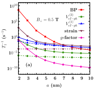
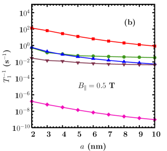
Figure 1: (Color online) $T_{1}^{-1}$ induced by different mechanisms vs. the well width for (a): perpendicular magnetic field $B_{\perp}=0.5$ T with (solid curves) and without (dashed curves) the SOC; (b) parallel magnetic field $B_{\|}=0.5$ T with the SOC. The effective diameter $d_{0}=20$ nm, and temperature $T=4$ K. Curves with $\blacksquare$ — $T_{1}^{-1}$ induced by the electron-BP scattering together with the SOC; Curves with $\bullet$ — $T_{1}^{-1}$ induced by the second-order process of the hyperfine interaction together with the BP ($V_{eI-ph}^{(3)}$); Curves with $\blacktriangle$ — $T_{1}^{-1}$ induced by the first-order process of the hyperfine interaction together with the BP ($V_{eI-ph}^{(1)}$); Curves with $\blacktriangledown$ — $T_{1}^{-1}$ induced by the direct spin-phonon coupling due to phonon-induced strain; Curves with $\blacklozenge$ — $T_{1}^{-1}$ induced by the $g$-factor fluctuation.

III.1.1 Well width dependence

In Fig. 1(a) and (b), the spin relaxation times induced by different mechanisms are plotted as function of the width of the quantum well in which the QD is confined for perpendicular magnetic field $B_{\perp}=0.5$ T and parallel magnetic field $B_{\|}=0.5$ T respectively. We first concentrate on the perpendicular magnetic field case. In Fig. 1(a), the calculation indicates that the spin relaxation due to each mechanism decreases with the increase of well width. Particularly the electron-BP scattering mechanism decreases much faster than the other mechanisms. It is indicated in the figures that when the well width is small (smaller than 7 nm in the present case), the spin relaxation time is determined by the electron-BP scattering together with the SOC. However, for wider well widths, the direct spin-phonon coupling due to phonon-induced strain and the first-order process of hyperfine interaction combined with the electron-BP scattering becomes more important. The decrease of spin relaxation due to each mechanism is mainly caused by the decrease of the SOC which is proportional to $a^{-2}$. The SOC has two effects which are crucial. First, in the second order perturbation the SOC contributes a finite correction to the Zeeman splitting which determines the absorbed/emitted phonon frequency and wave-vector.Cheng Second, it leads to spin mixing. The decrease of the SOC thus leads to the decrease of Zeeman splitting and spin mixing. The former leads to small phonon wave-vector and small phonon absorption/emission efficiency.Cheng Therefore the electron-BP mechanism decreases rapidly with increasing $a$. On the other hand, the other two largest mechanisms can flip spin without the help of the SOC. The spin relaxations due to these two mechanisms decrease in a relatively mild way. It is further confirmed that without SOC they decreases in a much milder way with increasing $a$ (dashed curves in Fig. 1). It is also noted that the spin relaxation rate due to the $g$-factor fluctuation is at least six orders of magnitude smaller than that due to the leading spin decoherence mechanisms and can therefore be neglected.

It is noted that in the calculation, the SOC is always included as it has large effect on the eigen-energy and eigen-wavefunction of the electron.Cheng We also show the spin relaxation times induced by the hyperfine interactions ($V^{(1)}_{eI-ph}$ and $V^{(3)}_{eI-ph}$) and the direct spin-phonon coupling due to the phonon-induced strain but without the SOC as in the literature.Erlingsson ; Abalmassov ; Kim It can be seen clearly that the spin relaxation that includes the SOC is much larger than that without the SOC. For example, the spin relaxation induced by the second-order process of the hyperfine interaction together with the BP ($V_{eI-ph}^{(3)}$) is at least one order of magnitude larger when the SOC is included than that when the SOC is neglected. This is because when the SOC is neglected, $\langle m|H_{eI}({\mathbf{r}})|\ell_{1}\rangle$ and $\langle\ell_{2}|H_{eI}({\mathbf{r}})|m\rangle$ in Eq. (29) are small as the matrix elements of $H_{eI}({\mathbf{r}})$ between different orbital energy levels are very small. However, when the SOC is taken into account, the spin-up and -down levels with different orbital quantum numbers are mixed and therefore $|\ell\rangle$ and $|m\rangle$ include the components with the same orbital quantum number. Consequently the matrix elements of $\langle m|H_{eI}({\mathbf{r}})|\ell_{1}\rangle$ and $\langle\ell_{2}|H_{eI}({\mathbf{r}})|m\rangle$ become much larger. Therefore, spin relaxation induced by this mechanism depends crucially on the SOC.

It is emphasized from the above discussion that the SOC should be included in each spin relaxation mechanism. In the following calculations it is always included unless otherwise specified. In particular in reference to the mechanism of electron-BP interaction, we always consider it together with the SOC.

We further discuss the parallel magnetic field case. In Fig. 1(b) the spin relaxation times due to different mechanisms are plotted as function of the quantum well width for same parameters as Fig. 1(a), but with a parallel magnetic field $B_{\|}=0.5$ T. It is noted that the spin relaxation rate due to each mechanism becomes much smaller for small $a$ compared with the perpendicular case. Another feature is that the spin relaxation due to each mechanism decrease in a much slower rate with increasing $a$. The electron-BP mechanism is dominant even at $a=10$ nm but decrease faster than other mechanisms with $a$. It is expected to be less effective than the $V_{eI-ph}^{(3)}$ mechanism or $V_{eI-ph}^{(1)}$ mechanism or the direct spin-phonon coupling due to phonon-induced strain mechanism for large enough $a$. The $g$-factor fluctuation mechanism is negligible again. These features can be explained as follows. For parallel magnetic field the contribution of the SOC to Zeeman splitting is much less than in the perpendicular magnetic field geometry.Destefani Moreover, this contribution is negative which makes Zeeman splitting smaller.Destefani Therefore, the phonon absorption/emission efficiency becomes much smaller for small $a$, i.e., large SOC. When $a$ increases, the Zeeman splitting increases. However, the spin mixing decreases. The former effect is weak, and only cancels part of the latter, thus the spin relaxation due to each mechanism decrease slowly with $a$.

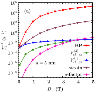
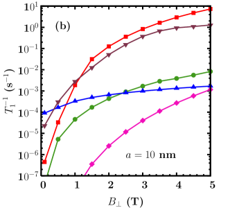
Figure 2: (Color online) $T_{1}^{-1}$ induced by different mechanisms vs. the perpendicular magnetic field $B_{\perp}$ for $d_{0}=20$ nm and (a) $a=5$ nm and (b) $10$ nm. $T=4$ K. Curves with $\blacksquare$ — $T_{1}^{-1}$ induced by the electron-BP scattering; Curves with $\bullet$ — $T_{1}^{-1}$ induced by the second-order process of the hyperfine interaction together with the BP ($V_{eI-ph}^{(3)}$); Curves with $\blacktriangle$ — $T_{1}^{-1}$ induced by the first-order process of the hyperfine interaction together with the BP ($V_{eI-ph}^{(1)}$); Curves with $\blacktriangledown$ — $T_{1}^{-1}$ induced by the direct spin-phonon coupling due to phonon-induced strain; Curves with $\blacklozenge$ — $T_{1}^{-1}$ induced by the $g$-factor fluctuation.

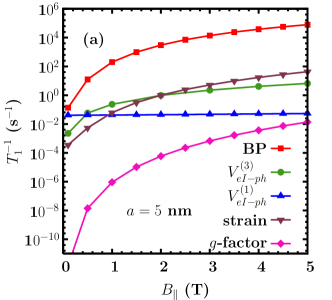
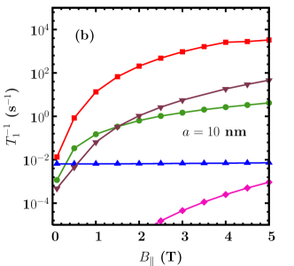
Figure 3: (Color online) $T_{1}^{-1}$ induced by different mechanisms vs. the parallel magnetic field $B_{\|}$ for $d_{0}=20$ nm and (a) $a=5$ nm and (b) $10$ nm. $T=4$ K. Curves with $\blacksquare$ — $T_{1}^{-1}$ induced by the electron-BP scattering; Curves with $\bullet$ — $T_{1}^{-1}$ induced by the second-order process of the hyperfine interaction together with the BP ($V_{eI-ph}^{(3)}$); Curves with $\blacktriangle$ — $T_{1}^{-1}$ induced by the first-order process of the hyperfine interaction together with the BP ($V_{eI-ph}^{(1)}$); Curves with $\blacktriangledown$ — $T_{1}^{-1}$ induced by the direct spin-phonon coupling due to phonon-induced strain; Curves with $\blacklozenge$ — $T_{1}^{-1}$ induced by the $g$-factor fluctuation.

III.1.2 Magnetic Field Dependence

We first study the perpendicular-magnetic-field case. The magnetic field dependence of $T_{1}$ for two different well widths are shown in Fig. 2(a) and Fig. 2(b). In the calculation, $d_{0}=20$ nm. It can be seen that the effect of each mechanism increases with the magnetic field. Particularly the electron-BP mechanism increases much faster than other ones and becomes dominant at high magnetic fields. For small well width (5 nm in Fig. 2a), the spin relaxation induced by the electron-BP scattering is dominant except at very low magnetic fields (0.1 T in the figure) where contributions from the first-order process of hyperfine interaction together with the electron-BP scattering and the direct spin-phonon coupling due to phonon-induced strain also contribute. It is interesting to see that when $a$ is increased to $10$ nm, the electron-BP scattering is the largest spin relaxation mechanism only at high magnetic fields ($>$1.1 T). For 0.4 T $<B_{\perp}<1.1$ T ($B_{\perp}<0.4$ T), the direct spin-phonon coupling due to the phonon-induced strain (the first order hyperfine interaction together with the BP ) becomes the largest relaxation mechanism. It is also noted that there is no single mechanism which dominates the whole spin relaxation. Two or three mechanisms are jointly responsible for the spin relaxation. It is indicated that the spin relaxations induced by different mechanisms all increase with $B_{\perp}$. This can be understood from a perturbation theory: when the magnetic field is small the spin relaxation between two Zeeman split states for each mechanism is proportional to $\bar{n}(\Delta E)(\Delta E)^{m}$ ($\Delta E$ is the Zeeman splitting) with $m=7$ for electron-BP scattering due to the deformation potentialCheng ; Stano2 and for the second-order process of the hyperfine interaction together with the electron-BP scattering due to the deformation potential $V_{eI-ph}^{(3)}$;Erlingsson $m=5$ for electron-BP scattering due to the piezoelectric couplingNazarov ; Cheng ; Stano2 and for the second-order process of the hyperfine interaction together with the electron-BP scattering due to the piezoelectric coupling $V_{eI-ph}^{(3)}$;Erlingsson and $m=5$ for the direct spin-phonon coupling due to phonon-induced strain;Nazarov $m=1$ for the first-order process of the hyperfine interaction together with the BP $V_{eI-ph}^{(1)}$. The spin relaxation induced by the $g$-factor fluctuation is proportional to $\bar{n}(\Delta E)(\Delta E)^{5}B_{\perp}^{2}$. For most of the cases studied, $\Delta E$ is smaller than $k_{B}T$, hence $\bar{n}(\Delta E)\sim k_{B}T/\Delta E$, and $\bar{n}(\Delta E)(\Delta E)^{m}\sim(\Delta E)^{m-1}$. $m>1$ hold for all mechanism except the $V_{eI-ph}^{(1)}$ mechanism, therefore the spin relaxation due to these mechanisms increases with increasing $B_{\perp}$. However, from Eq. (27) one can see that it has a term with ${\mathbf{\nabla}}_{{\mathbf{r}}}$, which indicates that the effect of this mechanism is proportional to $1/d_{0}$. As the vector potential of the magnetic field increases the confinement of the QD and gives rise to smaller effective diameter $d_{0}$, this mechanism also increases with the magnetic field in the perpendicular magnetic field geometry.

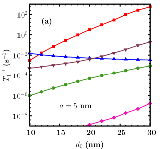
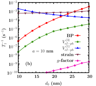
Figure 4: (Color online) $T_{1}^{-1}$ induced by different mechanisms vs. the effective diameter $d_{0}$ for $B_{\perp}=0.5$ T and (a) $a=5$ nm and (b) $10$ nm. $T=4$ K. Curves with $\blacksquare$ — $T_{1}^{-1}$ induced by the electron-BP scattering; Curves with $\bullet$ – $T_{1}^{-1}$ induced by the second-order process of the hyperfine interaction together with the BP ($V_{eI-ph}^{(3)}$); Curves with $\blacktriangle$ — $T_{1}^{-1}$ induced by the first-order process of the hyperfine interaction together with the BP ($V_{eI-ph}^{(1)}$); Curves with $\blacktriangledown$ — $T_{1}^{-1}$ induced by the direct spin-phonon coupling due to phonon-induced strain; Curves with $\blacklozenge$ — $T_{1}^{-1}$ induced by the $g$-factor fluctuation.

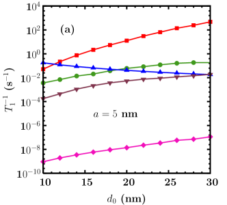
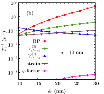
Figure 5: (Color online) $T_{1}^{-1}$ induced by different mechanisms vs. the effect diameter $d_{0}$ with $B_{\|}=0.5$ T and (a) $a=5$ nm and (b) $10$ nm. $T=4$ K. Curves with $\blacksquare$ — $T_{1}^{-1}$ induced by the electron-BP scattering; Curves with $\bullet$ — $T_{1}^{-1}$ induced by the second-order process of the hyperfine interaction together with the BP ($V_{eI-ph}^{(3)}$); Curves with $\blacktriangle$ — $T_{1}^{-1}$ induced by the first-order process of the hyperfine interaction together with the BP ($V_{eI-ph}^{(1)}$); Curves with $\blacktriangledown$ — $T_{1}^{-1}$ induced by the direct spin-phonon coupling due to phonon-induced strain; Curves with $\blacklozenge$ — $T_{1}^{-1}$ induced by the $g$-factor fluctuation.

We then study the case with the magnetic field parallel to the quantum well plane. In Fig. 3 the spin relaxation induced by different mechanisms are plotted as function of the parallel magnetic field $B_{\|}$ for two different well widths. In the calculation, $d_{0}=20$ nm. It can be seen that, similar to the case with perpendicular magnetic field, the effects of most mechanisms increase with the magnetic field. Also the electron-BP mechanism increases much faster than the other ones and becomes dominant at high magnetic fields. However, without the orbital effect of the magnetic field in the present configuration, the effect of $V_{eI-ph}^{(1)}$ changes very little with the magnetic field. For both small ($5$ nm in Fig. 3(a)) and large ($10$ nm in Fig. 3(b)) well widths, the electron-BP scattering is dominant except at very low magnetic field ($0.1$ T in the figure), where the first-order process of the hyperfine interaction together with the electron-BP interaction $V_{eI-ph}^{(1)}$ also contributes.

III.1.3 Diameter Dependence

We now turn to the investigation of the diameter dependence of the spin relaxation. We first concentrate on the perpendicular magnetic field geometry. The spin relaxation rate due to each mechanism is shown in Fig. 4a for a small ($a=5$ nm) and Fig. 4b for a large ($a=10$ nm) well widths respectively with a fixed perpendicular magnetic field $B_{\perp}=0.5$ T. In the figure, the spin relaxation rate due each mechanism except $V_{eI-ph}^{(1)}$ increases with the effective diameter. Specifically, the effect of the electron-BP mechanism increases very fast, while the effect of the direct spin-phonon coupling due to phonon-induced strain mechanism increases very mildly. The $V_{eI-ph}^{(1)}$ decreases with $d_{0}$ slowly. Other mechanisms are unimportant. The electron-BP mechanism eventually dominates spin relaxation when the diameter is large enough. The threshold increases from 12 nm to 26 nm when the well width increases from 5 nm to 10 nm. For small diameter the $V_{eI-ph}^{(1)}$ and the direct spin-phonon coupling due to phonon-induced strain mechanism dominate the spin relaxation. The increase/decrease of the spin relaxation due to these mechanisms can be understood from the following. The effect of the SOC on the Zeeman splitting is proportional to $d_{0}^{2}$ for small magnetic field.Cheng The increase of $d_{0}$ thus leads to a increase of Zeeman splitting, therefore the efficiency of the phonon absorption/emission increases. Another effect is that the increase of $d_{0}$ will increase the phonon absorption/emission efficiency due to the increase of the form factor.Cheng Thus the spin relaxation increases. Moreover, the spin mixing is also proportional to $d_{0}$ also.Cheng This leads to much faster increasing of the effect of the electron-BP mechanism and the $V_{eI-ph}^{(3)}$ mechanism. However, the spin relaxation due to $V_{eI-ph}^{(1)}$ decreases with the diameter. This is because $V_{eI-ph}^{(1)}$ contains a term ${\mathbf{\nabla}}_{{\mathbf{r}}}$ [Eq. (27)] which decreases with the increase of $d_{0}$. Physically speaking, the decrease of the effect of $V_{eI-ph}^{(1)}$ is due to the fact that the spin mixing due to the hyperfine interaction decreases with the increase of the number of nuclei within the dot $N$ as the random Overhauser field is proportional to $1/\sqrt{N}$. The spin relaxation induced by the $g$-factor is also negligible here for both small and large well width.

We then turn to the parallel magnetic field case. In the calculation, $B_{\|}=0.5$ T. The results are shown for both small well width ($a=5$ nm in Fig. 5(a)) and large well width ($a=10$ nm in Fig. 5(b)) respectively. Similar to the perpendicular magnetic field case, the effect of every mechanism except the $V_{eI-ph}^{(1)}$ mechanism increases with increasing diameter. The effect of the electron-BP mechanism increases fastest and becomes dominant for $d_{0}>12$ nm for both small and large well width. For $d_{0}<12$ nm for the two cases the first-order process of the $V_{eI-ph}^{(1)}$ mechanism becomes dominant. The effect of the $V_{eI-ph}^{(3)}$ mechanism become larger than that of the direct spin-phonon coupling due to phonon-induced strain mechanism. However, these two mechanism are still unimportant and becomes more and more unimportant for larger $d_{0}$. Here, the spin relaxation induced by the $g$-factor is negligible.

III.1.4 Comparison with Experiment

In this subsection, we apply our analysis to experiment data in Ref. Elzerman, . We first show that our calculation is in good agreement with the experimental results. Then we compare contributions from different mechanisms to spin relaxation as function of the magnetic field. In the calculation we choose the quantum dot diameter $d_{0}=56$ nm ($\hbar\omega_{0}=1.1$ meV as in experiment). The quantum well is taken to be an infinite-depth well with $a=13$ nm. The Dresselhaus SOC parameter $\gamma_{0}\langle k_{z}^{2}\rangle$ is taken to be 4.5 meV$\cdot$Åand the Rashba SOC parameter is 3.3 meV$\cdot$Å. $T=0$ K as $k_{B}T\ll g\mu_{B}B$ in the experiment. The magnetic field is applied parallel to the well plane in [110]-direction. The Dresselhaus cubic term is also taken into consideration. All these parameters are the same with (or close to) those used in Ref. Stano, in which a calculation based on the electron-BP scattering mechanism agrees well with the experimental results. For this mechanism, we reproduce their results. The spin relaxation time measured by the experiments (black dots with error bar in the figure) almost coincide with the calculated spin relaxation time due to the electron-BP scattering mechanism (curves with $\blacksquare$ in the figure).note2 It is noted from the figure that other mechanisms are unimportant for small magnetic field. However, for large magnetic field the effect of the direct-spin phonon coupling due to phonon-induced strain becomes comparable with that of the electron-BP mechanism. At $B_{\|}=10$ T, the two differs by a factor of $\sim 5$.

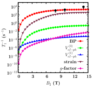
Figure 6: (Color online) $T_{1}^{-1}$ induced by different mechanisms vs. the parallel magnetic field $B_{\|}$ in the [110] direction for $d_{0}=56$ nm and $a=13$ nm with both the Rashba and Dresselhaus SOCs. $T=0$ K. The black dots with error bar is the experimental results in Ref. Elzerman, . Curves with $\blacksquare$ — $T_{1}^{-1}$ induced by the electron-BP scattering; Curves with $\bullet$ — $T_{1}^{-1}$ induced by the second-order process of the hyperfine interaction together with the BP ($V_{eI-ph}^{(3)}$); Curves with $\blacktriangle$ — $T_{1}^{-1}$ induced by the first-order process of the hyperfine interaction together with the BP ($V_{eI-ph}^{(1)}$); Curves with $\blacktriangledown$ — $T_{1}^{-1}$ induced by the direct spin-phonon coupling due to phonon-induced strain; Curves with $\blacklozenge$ — $T_{1}^{-1}$ induced by the $g$-factor fluctuation.

III.2 Spin Dephasing Time $T_{2}$

In this subsection, we investigate the spin dephasing time for different well widths, magnetic fields and QD diameters. As in the previous subsection, the contributions of the different mechanisms to spin dephasing are compared.note1 To justify the first Born approximation in studying the hyperfine interaction induced spin dephasing, we focus mainly on the high magnetic field regime of $B>3.5$ T. A typical magnetic field is $4$ T. We also demonstrate via extrapolation that in the low magnetic field regime spin dephasing is dominated by the hyperfine interaction.

III.2.1 Well Width Dependence

In Fig. 7 the well width dependence of the spin dephasing induced by different mechanisms is presented under the perpendicular (a) and parallel (b) magnetic fields. In the calculations $B_{\perp}=4$ T/$B_{\|}=4$ T and $d_{0}=20$ nm. It can be seen in both figures that the spin dephasing due to each mechanism decreases with $a$. Moreover, the spin dephasing due to the electron-BP scattering decreases much faster than that due to the hyperfine interaction. These features can be understood as following. The spin dephasing due to electron-BP scattering depends crucially on the SOC. As the SOC is proportional to $a^{-2}$, the spin dephasing decreases fast with $a$. For the hyperfine interaction, from Eq. (35) one can deduce that the decay rate of $||\langle S_{+}\rangle_{t}||$ is mainly determined by the factor $1/(a_{z}d_{\|}^{2})$ (here $a_{z}=a$), which thus decreases with $a$, but in a very mild way. The fast decrease of the electron-BP mechanism makes it eventually unimportant. For the present perpendicular-magnetic-field case the threshold is around 2 nm. For parallel magnetic field it is even smaller. A higher temperature may enhance the electron-BP mechanism (see discussion in Sec. V) and make it more important than the hyperfine mechanism. It is noted that other mechanisms contribute very little to the spin dephasing. Thus, in the following discussion, we do not consider these mechanisms. Comparing Figs 7(a) and (b), one finds that a main difference is that the electron-BP mechanism is less effective for the parallel-magnetic-field case. As has been discussed in the previous subsection, the spin mixing and the Zeeman splitting in the parallel filed case is smaller than those in the perpendicular field case. Therefore, the electron-BP mechanism is weakened markedly.

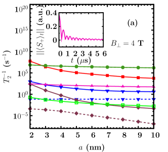
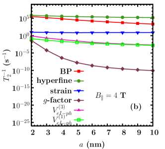
Figure 7: (Color online) $T_{2}^{-1}$ induced by different mechanisms vs. the well width for $d_{0}=20$ nm. $T=4$ K. (a): $B_{\perp}=4$ T with (solid curves) and without (dashed curves) the SOC; (b): $B_{\|}=4$ T only with the SOC. Curve with $\blacksquare$ — $T_{2}^{-1}$ induced by the electron-BP interaction; Curves with $\bullet$ — $T_{2}^{-1}$ induced by the hyperfine interaction; Curves with $\blacktriangledown$ — $T_{2}^{-1}$ induced by the direct spin-phonon coupling due to phonon-induced strain; Curves with $\blacklozenge$ — $T_{2}^{-1}$ induced by $g$-factor fluctuation; $\blacktriangle$ — $T_{2}^{-1}$ induced by the second-order process of the hyperfine interaction together with the BP ($V_{eI-ph}^{(3)}$); Curves with $\square$ — $T_{2}^{-1}$ induced by the first-order process of the hyperfine interaction together with the BP ($V_{eI-ph}^{(1)}$). The time evolution of $||\langle S_{+}\rangle_{t}||$ induced by the hyperfine interaction with $a=2$ nm is shown in the inset of (a).

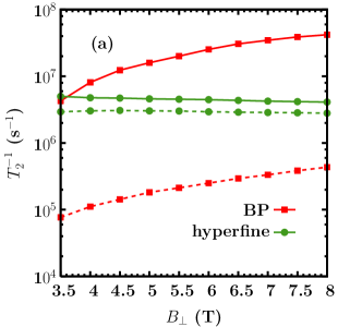
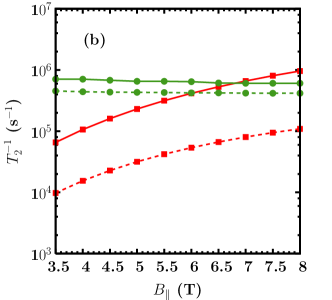
Figure 8: (Color online) $T_{2}^{-1}$ induced by the electron-BP scattering and the hyperfine interaction vs. (a): the perpendicular magnetic field $B_{\perp}$ ; (b): the parallel magnetic field $B_{\|}$ for $a=3$ nm (solid curves) and $5$ nm (dashed curves). $T=4$ K, and $d_{0}=20$ nm. Curves with $\blacksquare$ — $T_{2}^{-1}$ induced by the electron-BP interaction; Curves with $\bullet$ — $T_{2}^{-1}$ induced by the hyperfine interaction.

Similar to Fig. 1, the SOC is always included in the computation as it has large effect on the eigen-energy and eigen-wavefunction of the electrons. The spin dephasings calculated without the SOC for the hyperfine interaction, the direct spin-phonon coupling due to phonon-induced strain and the $g$-factor fluctuation are also shown in Fig. 7(a) as dashed curves. It can be seen from the figure that for the spin dephasings induced by the direct spin-phonon coupling due to phonon-induced strain and by the $g$-factor fluctuation, the contributions with the SOC are much larger than those without. This is because when the SOC is included, the fluctuation of the effective field induced by both mechanisms becomes much stronger and more scattering channels are opened. However, what should be emphasized is that the spin dephasings induced by the hyperfine interaction with and without the SOC are nearly the same (the solid and the dashed curves nearly coincide). That is because the change of the wavefunction $\Psi({\bf r})$ due to the SOC is very small (less than 1 % in our condition) and therefore the factor $1/(a_{z}d_{\|}^{2})$ is almost unchanged when the SOC is neglected. Thus the spin dephasing rate is almost unchanged.

In the inset of Fig. 7(a), the time evolution of $||\langle S_{+}\rangle_{t}||$ induced by the hyperfine interaction is shown, with $a=2$ nm. It can be seen that $||\langle S_{+}\rangle_{t}||$ decays very fast and decreases to less than 10 % of its initial value within the first two oscillating periods. Therefore, $T_{2}$ is determined by the first two or three periods of $||\langle S_{+}\rangle_{t}||$. Thus the correction of the long time dynamics due to higher order scatteringCoish contributes little to the spin dephasing time. For quantum computation and quantum information processing, the initial, e.g., 1 % decay of $||\langle S_{+}\rangle_{t}||$ may be more important than the $1/e$ decay.Yao ; Witzel2 Indeed, the spin dephasing time defined by the exponential fitting of 1 % decay is short than that defined by the $1/e$ decay. However, the two differs less than 5 times. For a rough comparison of contributions from different mechanisms to spin dephasing where only the order-of-magnitude difference is concerned (see Figs. 7-9), this difference due to the definition does not jeopardize our conclusions.

III.2.2 Magnetic Field Dependence

We then investigate the magnetic field dependence of the spin dephasing induced by the electron-BP scattering and by the hyperfine interaction for two different well widths ($a=3$ nm and $a=5$ nm) with both perpendicular and parallel magnetic field. From Fig. 8(a) and (b) one can see that the spin dephasing due to the electron-BP scattering increases with magnetic field, whereas that due to the hyperfine interaction decreases with magnetic field. Thus, the electron-BP mechanism eventually dominates the spin dephasing for high enough magnetic field. The threshold is $B_{\perp}^{c}=4$ T / $B_{\|}^{c}=7$ T for $a=3$ nm with perpendicular/parallel magnetic field. For larger well width, e.g., $a=5$ nm with parallel magnetic field or perpendicular magnetic field, the threshold magnetic fields increase to larger than $8$ T. The different magnetic field dependences above can be understood as following. Besides spin relaxation, the spin-flip scattering also contributes to spin dephasing.Golovach As has been demonstrated in Sec. IIIA, the electron-BP scattering induced spin-flip transition rate increases with the magnetic field. Therefore the spin dephasing rate increases with the magnetic field also. In contrast, spin dephasing induced by the hyperfine interaction decreases with the magnetic field. This is because when the magnetic field becomes larger, the fluctuation of the effective magnetic field due to the surrounding nuclei becomes insignificant compared. Therefore, the hyperfine-interaction-induced spin dephasing is reduced. Similar results have been obtained by Deng and Hu.Deng2

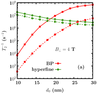
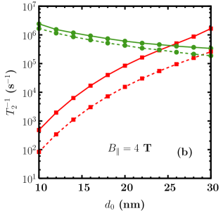
Figure 9: (Color online) $T_{2}^{-1}$ induced by the electron-BP scattering and the hyperfine interaction vs. the effective diameter $d_{0}$ $T=4$ K. (a): $B_{\perp}=4$ T ; (b): $B_{\|}=4$ T for $a=3$ nm (solid curves) and $5$ nm (dashed curves). Curves with $\blacksquare$ — $T_{2}^{-1}$ induced by the electron-BP interaction; Curves with $\bullet$ — $T_{2}^{-1}$ induced by the hyperfine interaction.

III.2.3 Diameter Dependence

In Fig. 9 the spin dephasing times induced by the electron-BP scattering and the hyperfine interaction are plotted as function of the diameter $d_{0}$ for a small ($a=3$ nm) and a large ($a=5$ nm) well widths. In the calculation, $B_{\perp}=4$ T in Fig. 9(a) and $B_{\|}=4$ T in (b). It is noted that the effect of the electron-BP mechanism increases rapidly with $d_{0}$, whereas the effect of the hyperfine mechanism decreases slowly. Consequently, the electron-BP mechanism eventually dominates the spin dephasing for large enough $d_{0}$. The threshold is $d_{0}^{c}=19$ (27) nm for $a=3$ (5) nm case with the perpendicular magnetic field and $d_{0}^{c}=26$ (30) nm for $a=3$ (5) nm case under the parallel magnetic field. As has been discussed in Sec. IIIA, both the effect of the SOC and the efficiency of the phonon absorption/emission increase with $d_{0}$. Therefore, the spin dephasing due to the electron-BP mechanism increases rapidly with $d_{0}$.Cheng ; Destefani The decrease of the effect of the hyperfine interaction is due to the decrease of the factor $1/(a_{z}d_{\|}^{2})$ [Eq. 35] with the diameter $d_{0}$.

IV spin relaxation times from Fermi Golden rule and from Equation of motion

In this section, we will try to find a proper method to average over the transition rates from the Fermi Golden rule, $\tau_{i\to f}^{-1}$, to give the spin relaxation time $T_{1}$. In the limit of small SOC, we rederive Eq. (1) from the equation of motion. We further show that Eq. (1) fails for large SOC where a full calculation from the equation of motion is needed.

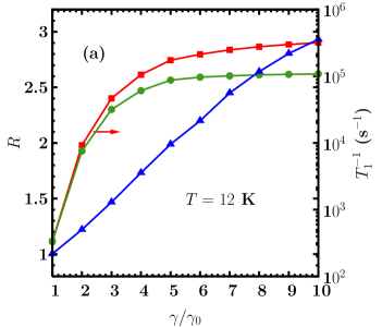
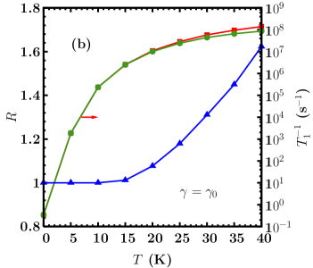
Figure 10: (Color online) Spin relaxation time $T_{1}$ calculated from the equation-of-motion approach ($\blacksquare$) v.s. that obtained from Eq. (1) ($\bullet$) as function of (a): the strength of the SOC for T=12 K; (b): the temperature for $\gamma=\gamma_{0}$. The well width $a=5$ nm, perpendicular magnetic field $B_{\perp}=0.5$ T, QD diameter $d_{0}=30$ nm. The ratio of the two $R$ is also plotted in the figure. Note the scale of $T_{1}^{-1}$ is at the right hand side of the frame.

We first rederive Eq. (1) for small SOC from the equation of motion. In QDs, the orbital level splitting is usually much larger than the Zeeman splitting. Each Zeeman sublevel has two states: one with majority up-spin, the other with majority down-spin. We call the former “minus state” (as it corresponds to a lower energy) while the latter “plus state”. For small SOC, the spin mixing is small. Thus we neglect the much smaller contribution from the off-diagonal terms of the density matrix to $S_{z}$. Therefore $S_{z}(t)=\sum_{i\pm}S_{z}^{i\pm}f_{i\pm}(t)$ where $i\pm$ denotes the plus/minus state of the $i$-th orbital state. For small SOC, the spin relaxation is much slower than the orbital relaxation.Fujisawa ; Stano2 This implies that the time takes to establish equilibrium within the plus/minus states is much smaller than the spin relaxation time. Thus we can assume a equilibrium (Maxwell-Boltzmann) distribution between the plus/minus states at any time. The distribution function is therefore given by $f_{i\pm}(t)=N_{\pm}(t)\exp(-\varepsilon_{i\pm}/k_{B}T)/Z_{\pm}$. Here $N_{\pm}(t)=\sum_{i}f_{i\pm}(t)$ is the total probability of the plus/minus states with $N_{+}(t)+N_{-}(t)=1$ for single electron in QD and $Z_{\pm}=\sum_{i}\exp(-\varepsilon_{i\pm}/k_{B}T)$ is the partition function for the plus/minus state. At equilibrium, $N_{\pm}=N_{\pm}^{eq}$. The equation for $S_{z}(t)$ is hence,

$$\frac{d}{dt}S_{z}(t) = \frac{d}{dt}[S_{z}(t)-S_{z}^{eq}]$$ (36)

$$= \sum_{i\pm}S_{z}^{i\pm}\exp(-\varepsilon_{i\pm}/k_{B}T)/Z_{\pm}\frac{d}{dt}\delta N_{\pm}(t)\ ,$$

with $\delta N_{\pm}(t)=N_{\pm}(t)-N_{\pm}^{eq}$. As the orbital level splitting is usually much larger than the Zeeman splitting, the factor $\exp(-\varepsilon_{i\pm}/k_{B}T)/Z_{\pm}$ can be approximated by $\exp(-\varepsilon_{i0}/k_{B}T)/Z_{0}$ with $\varepsilon_{i0}=\frac{1}{2}(\varepsilon_{i+}+\varepsilon_{i-})$ and $Z_{0}=\sum_{i}\exp[-\varepsilon_{i0}/k_{B}T]$. Further using the particle-conservation relation $\sum_{\pm}\delta N_{\pm}(t)=0$, one has

$$\frac{d}{dt}S_{z}(t)=[\sum_{i}(S_{z}^{i+}-S_{z}^{i-})\exp(-\varepsilon_{i0}/k_{B}T)/Z_{0}]\frac{d}{dt}\delta N_{+}(t)\ .$$ (37)

As $S_{z}(t)-S_{z}^{eq}=[\delta N_{+}(t)/Z_{0}]\sum_{i}(S_{z}^{i+}-S_{z}^{i-})\exp(-\varepsilon_{i0}/k_{B}T)$, one finds that the spin relaxation time is nothing but the relaxation time of $N_{+}$. The next step is to derive the equation of $\frac{d}{dt}\delta N_{+}(t)$, which is given in our previous work:JHJiang

$$\frac{d}{dt}\delta N_{+}(t)=\sum_{i}\frac{d}{dt}\delta f_{i+}(t)$$

$$=-\sum_{i,f}[\tau_{{i+}\to{f-}}^{-1}\delta f_{i+}(t)-\tau_{{i-}\to{f+}}^{-1}\delta f_{i-}(t)]$$

$$=-\sum_{i,f}[\tau_{{i+}\to{f-}}^{-1}+\tau_{{i-}\to{f+}}^{-1}]\frac{e^{-\varepsilon_{i0}/k_{B}T}}{Z_{0}}\delta N_{+}(t)\ .$$ (38)

Thus spin relaxation time is given by,

$$\frac{1}{T_{1}}=\sum_{i,f}(\tau_{{i+}\to{f-}}^{-1}+\tau_{{i-}\to{f+}}^{-1})\frac{e^{-\varepsilon_{i0}/k_{B}T}}{Z_{0}}\ .$$ (39)

Furthermore, substituting $e^{-\varepsilon_{i0}/k_{B}T}/Z_{0}$ by $f_{i\pm}^{0}=\exp(-\varepsilon_{i\pm}/k_{B}T)/Z_{\pm}$, we have

$$\frac{1}{T_{1}}=\sum_{i,f}(\tau_{{i+}\to{f-}}^{-1}f_{i+}^{0}+\tau_{{i-}\to{f+}}^{-1}f_{i-}^{0})\ .$$ (40)

This is exactly Eq. (1).

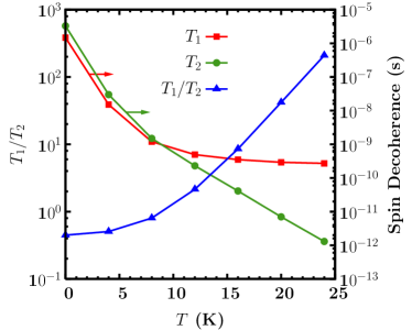
Figure 11: (Color online) Spin relaxation time $T_{1}$, spin dephasing time $T_{2}$ and $T_{1}/T_{2}$ against temperature $T$. $B_{\perp}=4$ T, $a=5$ nm and $d_{0}=30$ nm. Note the scale of $T_{1}$ and $T_{2}$ is at the right hand side of the frame.

For large SOC, or large spin mixing due to anticrossing of different spin states,Bulaev ; Stano2 the spin relaxation rate becomes comparable with the orbital relaxation rate. Furthermore, the decay of the off-diagonal term of the density matrix should contribute to the decay of $S_{z}$. Therefore, the above analysis does not hold. In this case, it is difficult to obtain such a formula, and a full calculation from the equation-of-motion is needed.

In Fig. 10(a), we show that (for $T=12$ K, $a=5$ nm, $B_{\perp}=0.5$ T, $d_{0}=30$ nm) the spin relaxation times $T_{1}$ calculated from equation-of-motion approach and that obtained from Eq. (40). Here, for simplicity and without loss of generality, we consider only the electron-BP scattering mechanism. The discrepancy of $T_{1}$ obtained from the two approaches increases with $\gamma$. At $\gamma=10\gamma_{0}$, the ratio of the two becomes as large as $\sim 3$. In Fig. 10(b), we plot the spin relaxation times obtained via the two approaches as function of temperature for $\gamma=\gamma_{0}$ with other parameters remaining unchanged. It is noted that the discrepancy of $T_{1}$ obtained from the two approaches increases with temperature. For high temperature, the higher levels are involved in the spin dynamics where the SOC becomes larger. At 40 K, the discrepancy is as large as 60 %. The ratio increases very slowly for $T<20$ K where only the lowest two Zeeman sublevels are involved in the dynamics.

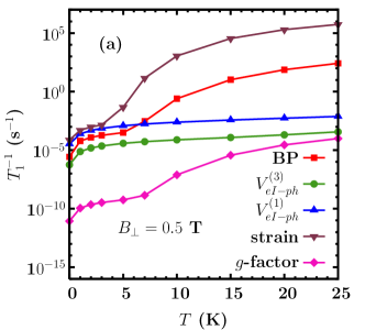
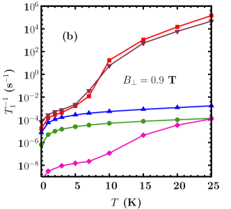
Figure 12: (Color online) Spin relaxation time $T_{1}$ against temperature $T$ for (a): $B_{\perp}=0.5$ T; (b): $B_{\perp}=0.9$ T. $a=10$ nm and $d_{0}=20$ nm. Curves with $\blacksquare$ — $T_{1}^{-1}$ induced by the electron-BP scattering together with the SOC; Curves with $\bullet$ — $T_{1}^{-1}$ induced by the second-order process of the hyperfine interaction together with the BP ($V_{eI-ph}^{(3)}$); Curves with $\blacktriangle$ — $T_{1}^{-1}$ induced by the first-order process of the hyperfine interaction together with the BP ($V_{eI-ph}^{(1)}$); Curves with $\blacktriangledown$ — $T_{1}^{-1}$ induced by the direct spin-phonon coupling due to phonon-induced strain; Curves with $\blacklozenge$ — $T_{1}^{-1}$ induced by the $g$-factor fluctuation.

V Temperature Dependence of Spin relaxation time $T_{1}$ and spin dephasing time $T_{2}$

We first study the relative magnitude of the spin relaxation time $T_{1}$ and the spin dephasing time $T_{2}$. We consider a QD with $d_{0}=30$ nm and $a=5$ nm at $B_{\perp}=4$ T where the largest contribution to both spin relaxation and dephasing comes from the electron-BP scattering (see Fig. 4(a) and Fig. 9(a), we have checked that the electron-BP scattering mechanism is dominant throughout the temperature range). From Fig. 11, one finds that when the temperature is low ($T<5$ K in the figure), $T_{2}=2T_{1}$, which is in agreement with the discussion in Ref. Golovach, . However, $T_{1}/T_{2}$ increases very quickly with $T$ and for $T=20$ K, $T_{1}/T_{2}\sim 2\times 10^{2}$. This is understood from the fact that when $T$ is low, the electron mostly distributes in the lowest two Zeeman sublevels. For small SOC, Golovach et al. have shown via perturbation theory that phonon induces only the spin-flip noise in the leading order. Consequently, $T_{2}=2T_{1}$.Golovach When the temperature becomes comparable with the orbital level splitting $\hbar\omega_{0}$, the distribution over the upper orbital levels is not negligible any more. As mentioned previously, the SOC contributes a non-trivial part to the Zeeman splitting. Specifically, the second order energy correction due to the SOC contributes to the Zeeman splitting. The energy correction for different orbital levels is generally unequal (always larger for higher levels). When the electron is scattered by phonons randomly from one orbital state to another one with the same major spin polarization, the frequency of its precession around $z$ direction changes. Continuous scattering leads to random fluctuation of the precession frequency and thus leads to spin dephasing.Semenov ; Semenov3 Note that this fluctuation only leads to a phase randomization of $S_{+}$, but not flips the $z$ component spin $S_{z}$, i.e., not leads to spin relaxation. Therefore, the spin dephasing becomes stronger than the spin relaxation for high temperatures. Moreover, this effect increases with temperature rapidly as the distribution over higher levels and the phonon numbers both increase with temperature.

We further study the temperature dependence of spin relaxation for lower magnetic field and larger quantum well width where other mechanisms may be more important than the electron-BP mechanism. In Fig. 12(a), the spin relaxation time is plotted as function of temperature for $B_{\perp}=0.5$ T, $a=10$ nm and $d_{0}=20$ nm. It is seen from the figure that the direct spin-phonon coupling due to phonon-induced strain mechanism dominates the spin relaxation throughout the temperature range. It is also noted that for $T\leq 4$ K the spin relaxation rates induced by different mechanisms all increase with temperature according to the phonon number factor $2\bar{n}(E_{z1})+1$ with $E_{z1}$ being the Zeeman splitting of the lowest Zeeman sublevels. However, for $T>4$ K, the spin relaxation rates induced by the direct spin-phonon coupling due to phonon-induced strain and the electron-BP interaction increase rapidly with temperature, while the spin relaxation rates induced by $V_{eI-ph}^{(1)}$ and $V_{eI-ph}^{(3)}$ increase mildly according to $2\bar{n}(E_{z1})+1$ throughout the temperature range. These features can be understood as what follows. For $T\leq 4$ K, the distribution over the high levels is negligible. Only the lowest two Zeeman sublevels involve in the spin dynamics. The spin relaxation rates thus increase with $2\bar{n}(E_{z1})+1$ and the relative importance of each mechanism does not change. Therefore, our previous analysis on comparison of relative importance of different spin decoherence mechanisms at 4 K holds true for the range $0\leq T\leq 4$ K. When the temperature gets higher, the contribution from higher levels becomes more important. Although the distribution at the higher levels is still very small, for the direct spin-phonon coupling mechanism, the transition rates between the higher levels and that between higher levels and the lowest two sublevels are very large. For the electron-BP mechanism the transition rates between the higher levels are very large due to the large SOC in these levels. Therefore, the contribution from the higher levels becomes larger than that from the lowest two sublevels. Consequently, the increase of temperature leads to rapid increase of the spin relaxation rates. However, for the two hyperfine mechanisms: the $V_{eI-ph}^{(1)}$ and the $V_{eI-ph}^{(3)}$, the spin relaxation rates does not change much when the higher levels are involved. They thus increase by the phonon number factor.

In Fig. 12(b) we show the temperature dependence of the spin relaxation time for the same condition but with $B=0.9$ T. It is noted that the spin relaxation rate due to the electron-BP mechanism catches up with that induced by the direct spin-phonon coupling due to phonon-induced strain at $T=9$ K and becomes larger for higher temperature. This indicates that the temperature dependence of the two mechanisms are quite different.

In Fig. 13 we show the spin dephasing induced by electron-BP scattering and the hyperfine interaction as function of temperature for $B_{\perp}=4$ T, $a=10$ nm and $d_{0}=20$ nm. We choose the conditions so that the spin dephasing is dominated by the hyperfine interaction at low temperature. However, the effect of the electron-BP mechanism increases with temperature quickly while that of the hyperfine interaction remains nearly unchanged. The fast increase of the effect from the electron-BP scattering is due to three factors: 1) the increase of the phonon number; 2) the increase of scattering channels; and 3) the increase of the SOC induced spin mixing in higher levels. On the other hand, from Eq. 35, one can deduce that the spin dephasing rate of the hyperfine interaction depends mainly on the factor $1/(a_{z}d_{\|}^{2})$ with $a_{z}$/$d_{\|}^{2}$ is the characteristic length/area along the $z$ direction / in the quantum well plane. For higher levels, the $d_{\|}^{2}$ is larger, but only about a factor smaller than 10. Thus the effect of the hyperfine interaction increases very slowly with temperature.

It should be noted that in the above discussion, we neglected the two-phonon scattering mechanism,Glavin ; Semenov3 ; Nazarov which may be important at high temperature. The contribution of this mechanism should be calculated via the equation-of-motion approach developed in this paper, and compared with the contribution of other mechanisms showed here.

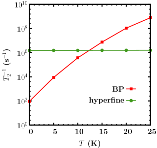
Figure 13: (Color online) Spin relaxation time $T_{1}$ against temperature $T$. $B_{\perp}=4$ T, $a=10$ nm and $d_{0}=20$ nm. Curves with $\blacksquare$ — $T_{2}^{-1}$ induced by the electron-BP scattering together with the SOC; Curves with $\bullet$ — $T_{2}^{-1}$ induced by the hyperfine interaction

VI Conclusion

In conclusion, we have investigated the longitudinal and transversal spin decoherence times $T_{1}$ and $T_{2}$, called spin relaxation time and spin dephasing time, in different conditions in GaAs QDs from the equation-of-motion approach. Various mechanisms, including the electron-BP scattering, the hyperfine interaction, the direct spin-phonon coupling due to phonon-induced strain and the $g$-factor fluctuation are considered. Their relative importance is compared. There is no doubt that for spin decoherence induced by electron-BP scattering, the SOC must be included. However, for spin decoherence induced by the hyperfine interaction, the direct spin-phonon coupling due to phonon-induced strain, $g$-factor fluctuation, and hyperfine interaction combined with electron-phonon scattering, the SOC is neglected in the existing literature.Erlingsson ; Abalmassov ; Kim Our calculations have shown that, as the SOC has marked effect on the eigen-energy and the eigen-wavefunction of the electron, the spin decoherence induced by these mechanisms with the SOC is larger than that without it. Especially, the decoherence from the second-order process of hyperfine interaction combined with the electron-BP interaction increases at least one order of magnitude when the SOC is included. Our calculations show that, with the SOC, in some conditions some of these mechanisms (except $g$-factor fluctuation mechanism) can even dominate the spin decoherence.

There is no single mechanism which dominates spin relaxation or spin dephasing in all parameter regimes. The relative importance of each mechanism varies with the well width, magnetic field and QD diameter. In particular, the electron-BP scattering mechanism has the largest contribution to spin relaxation and spin dephasing for small well width and/or high magnetic field and/or large QD diameter. However, for other parameters the hyperfine interaction, the first-order process of the hyperfine interaction combined with electron-BP scattering, and the direct spin-phonon coupling due to phonon-induced strain can be more important. It is noted that the $g$-factor fluctuation always has very little contribution to spin relaxation and spin dephasing which can thus be neglected all the time. For spin dephasing, the electron-BP scattering mechanism and the hyperfine interaction mechanism are more important than other mechanisms for magnetic field higher than 3.5 T. For this regime, other mechanisms can thus be neglected. It is also shown that spin dephasing induced by the electron-BP mechanism increases rapidly with temperature. Extrapolated from our calculation, the hyperfine interaction mechanism is believed to be dominant for small magnetic field.

We also discussed the problem of finding a proper method to average over the transition rates $\tau_{i\to f}^{-1}$ obtained from the Fermi Golden rule, to give the spin relaxation time $T_{1}$ at finite temperature. For small SOC, we rederived the formula for $T_{1}$ at finite temperature used in the existing literatureCheng ; lv ; Wang from the equation of motion. We further demonstrated that this formula is inadequate at high temperature and/or for large SOC. For such cases, a full calculation from the equation-of-motion approach is needed. The equation-of-motion approach provides an easy and powerful way to calculate the spin decoherence at any temperature and SOC.

We also studied the temperature dependence of spin relaxation $T_{1}$ and dephasing $T_{2}$. We show that for very low temperature if the electron only distributes on the lowest two Zeeman sublevels, $T_{2}=2T_{1}$. However, for higher temperatures, the electron spin dephasing increases with temperature much faster than the spin relaxation. Consequently $T_{1}\gg T_{2}$. The spin relaxation and dephasing due to different mechanisms are also compared.

- (1) Semiconductor Spintronics and Quantum Computation, edited by D. D. Awschalom, D. Loss, and N. Samarth (Springer-Verlag, Berlin, 2002); I. Zutic, J. Fabian, and S. Das Sarma, Rev. Mod. Phys. 76, 323 (2004).
- (2) H.-A. Engel, L. P. Kouwenhoven, D. Loss, and C. M. Marcus, Quantum Information Processing 3, 115 (2004); D. Heiss, M. Kroutvar, J. J. Finley, and G. Abstreiter, Solid State Commun. 135, 591 (2005); and references therein.
- (3) D. Loss and D. P. DiVincenzo, Phys. Rev. A 57, 120 (1998).
- (4) R. Hanson, L. P. Kouwenhoven, J. R. Petta, S. Tarucha, and L. M. K. Vandersypen, Rev. Mod. Phys. 79, 1217 (2007).
- (5) J. M. Taylor, H.-A. Engel, W. Dür, A. Yacoby, C. M. Marcus, P. Zoller, and M. D. Lukin, Nature Phys. 1, 177 (2005).
- (6) S. Amasha, K. MacLean, I. Radu, D. M. Zumbuhl, M. A. Kastner, M. P. Hanson, and A. C. Gossard, cond-mat/0607110.
- (7) J. M. Elzerman, R. Hanson, L. H. Willems van Beveren, B. Witkamp, L. M. K. Vandersypen and L. P. Kouwenhoven, Nature (London) 430, 431 (2004).
- (8) D. Paget, G. Lample, B. Sapoval, and V. I. Safarov, Phys. Rev. B 15, 5780 (1977).
- (9) Optical Orientation, edited by F. Meier and B. P. Zakharchenya (North-Holland, Amsterdam, 1984).
- (10) G. Dresselhaus, Phys. Rev. 100, 580 (1955).
- (11) Y. Bychkov and E. I. Rashba, J. Phys. C 17, 6039 (1984).
- (12) L. M. Roth, Phys. Rev. 118, 1534 (1960).
- (13) A. V. Khaetskii and Y. V. Nazarov, Physica E 6, 470 (2000).
- (14) A. V. Khaetskii and Y. V. Nazarov, Phys. Rev. B 61, 12639 (2000).
- (15) A. V. Khaetskii and Y. V. Nazarov, Phys. Rev. B 64, 125316 (2001).
- (16) L. M. Woods, T. L. Reinecke, and Y. Lyanda-Geller, Phys. Rev. B 66, 161318 (2002).
- (17) R. de Sousa and S. Das Sarma, Phys. Rev. B 68, 155330 (2003).
- (18) J. L. Cheng, M. W. Wu, and C. Lü, Phys. Rev. B 69, 115318 (2004).
- (19) D. V. Bulaev and D. Loss, Phys. Rev. B 71, 205324 (2005).
- (20) V. N. Golovach, A. Khaetskii, and D. Loss, Phys. Rev. Lett. 93, 016601 (2004).
- (21) C. F. Destefani and S. E. Ulloa, Phys. Rev. B 72, 115326 (2005).
- (22) P. San-Jose, G. Zarand, A. Shnirman, and G. Schön, Phys. Rev. Lett. 97, 076803 (2006).
- (23) V. I. Fal’ko, B. L. Altshuler, and O. Tsyplyatyev, Phys. Rev. Lett. 95, 076603 (2005).
- (24) P. Stano and J. Fabian, Phys. Rev. Lett. 96, 186602 (2006).
- (25) P. Stano and J. Fabian, Phys. Rev. B 74, 045320 (2006).
- (26) H. Westfahl. Jr., A. O. Caldeira, G. Medeiros-Ribeiro, and M. Cerro, Phys. Rev. B 70, 195320 (2004).
- (27) S. I. Erlingsson, and Yuli V. Nazarov, Phys. Rev. B 66, 155327 (2002).
- (28) V. A. Abalmassov and F. Marquardt, Phys. Rev. B 70, 075313 (2004).
- (29) Y. G. Semenov and K. W. Kim, Phys. Rev. Lett. 92, 026601 (2004).
- (30) A. V. Khaetskii, D. Loss, and L. Glazman, Phys. Rev. Lett. 88, 186802 (2002).
- (31) A. Khaetskii, D. Loss, and L. Glazman, Phys. Rev. B 67, 195329 (2003).
- (32) J. Schliemann, A. Khaetskii, and D. Loss, J. Phys.: Condens. Matter 15, R1809 (2003) and references there in.
- (33) W. A. Coish and D. Loss, Phys. Rev. B 70, 195340 (2004).
- (34) Ö. Cakir and T. Takagahara, cond-mat/0609217.
- (35) C. Deng and X. Hu, cond-mat/0608544.
- (36) S. I. Erlingsson and Yuli V. Nazarov, Phys. Rev. B 70, 205327 (2004).
- (37) N. Shenvi, R. de Sousa, and K. B. Whaley, Phys. Rev. B 71, 224411 (2005).
- (38) R. de Sousa, in Electron spin resonance and related phenomena in low dimensional structures, edited by M. Fanciulli (Springer-Verlag, Berlin, to be published.)
- (39) Y. V. Pershin and V. Privman, Nano Lett. 3, 695 (2003).
- (40) I. A. Merkulov, Al. L. Efros, and M. Rosen, Phys. Rev. B 65, 205309 (2002).
- (41) W. M. Witzel, R. de Sousa, and S. Das Sarma, Phys. Rev. B 72, 161306 (2005).
- (42) W. Yao, R.-B. Liu, and L. J. Sham, Phys. Rev. B 74, 195301 (2006).
- (43) W. M. Witzel and S. Das Sarma, Phys. Rev. B 74, 035322 (2006).
- (44) C. Deng and X. Hu, Phys. Rev. B 73, 241303 (2006).
- (45) Y. G. Semenov and K. W. Kim, Phys. Rev. B 70, 085305 (2004).
- (46) Y. G. Semenov and K. W. Kim, Phys. Rev. B 75, 195342 (2007).
- (47) W. M. Witzel and S. Das Sarma, Phys. Rev. Lett. 98, 077601 (2007).
- (48) R. de Sousa, N. Shenvi, and K. B. Whaley, Phys. Rev. B 72 045330 (2005).
- (49) J. H. Jiang and M. W. Wu, Phys. Rev. B 75, 035307 (2007).
- (50) B. A. Glavin and K. W. Kim, Phys. Rev. B 68, 045308 (2003).
- (51) C. Lü, J. L. Cheng, and M. W. Wu, Phys. Rev. B 71, 075308 (2005).
- (52) Y. Y. Wang and M. W. Wu, Phys. Rev. B 74, 165312 (2006).
- (53) W. H. Lau and M. E. Flatté, Phys. Rev. B 72, 161311(R) (2005).
- (54) C. P. Slichter, Principles of Magnetic Resonance, (Springer-Verlag, Berlin, 1990).
- (55) T. Fujisawa, D. G. Austing, Y. Tokura, Y. Hirayama, and S. Tarucha, Nature 419, 278 (2002).
- (56) see, e.g., P. N. Argyres and P. L. Kelley, Phys. Rev. 134, A98 (1964).
- (57) R. L. Fulton, J. Chem. Phys. 41, 2876 (1964).
- (58) P.-F. Braun, X. Marie, L. Lombez, B. Urbaszek, T. Amand, P. Renucci, V. K. Kalevich, K. V. Kavokin, O. Krebs, P. Voisin, and Y. Masumoto, Phys. Rev. Lett. 94, 116601 (2005).
- (59) F. H. L. Koppens, J. A. Folk, J. M. Elzerman, R. Hanson, L. H. Willems van Beveren, I. T. Vink, H. P. Tranitz, W. Wegscheider, L. P. Kouwenhoven, L. M. K. Vandersypen, Science 309, 1346 (2005).
- (60) J. R. Petta, A. C. Johnson, J. M. Taylor, E. A. Laird, A. Yacoby, M. D. Lukin, C. M. Marcus, M. P. Hanson, A. C. Gossard, Science 309, 2180 (2005).
- (61) F. H. L. Koppens, K. C. Nowack, and L. M. K. Vandersypen, arXiv:0711.0479.
- (62) M. W. Wu and H. Metiu, Phys. Rev. B 61, 2945 (2000).
- (63) T. Kuhn and F. Rossi, Phys. Rev. Lett. 69, 977 (1992).
- (64) J. Shah, Ultrafast Spectroscopy of Semiconductors and Semiconductor Nanostructures (Springer, Berlin, 1996).
- (65) M. I. D’yakonov and V. I. Perel’, Zh. Eksp. Teor. Fiz. 60, 1954 (1971) [Sov. Phys. JETP 33, 1053 (1971)].
- (66) A. Abragam, The Principles of Nuclear Magnetism (Oxford University Press, Oxford, 1961), Chaps. VI and IX.
- (67) This can be obtained from Eq. (17) in Ref. Yao, .
- (68) Numerical Data and Functional Relationships in Science and Technology, edited by O. Madelung, M. Schultz, and H. Weiss, Landolt-Börnstein, New Series, Group III, Vol. 17, Pt. a (Springer-Verlag, Berlin, 1982).
- (69) W. Knap, C. Skierbiszewski, A. Zduniak, E. Litwin-Staszewska, D. Bertho, F. Kobbi, J. L. Robert, G. E. Pikus, F. G. Pikus, S. V. Iordanskii, V. Mosser, K. Zekentes, and Yu. B. Lyanda-Geller, Phys. Rev. B 53, 3912 (1996).
- (70) It should be mentioned that one effect is not included : when electron is scattered by phonon from one orbital state to another, it feels a difference in the spin precession frequency since the strength of longitudinal (along the external magnetic field) component of Overhauser field differs with orbital states. This effect randomizes the spin precession phase and leads to a pure spin dephasing. However, this effect is negligible in our manuscript.
- (71) The deviation of our calculation from the experiment data at T is due to the fact that we do not include the cyclotron effect along the- direction. For T, the cyclotron orbit length is smaller than the quantum well width, which makes our model unrealistic.