Construction of initial data for 3+1 numerical relativity

Abstract

This lecture is devoted to the problem of computing initial data for the Cauchy problem of 3+1 general relativity. The main task is to solve the constraint equations. The conformal technique, introduced by Lichnerowicz and enhanced by York, is presented. Two standard methods, the conformal transverse-traceless one and the conformal thin sandwich, are discussed and illustrated by some simple examples. Finally a short review regarding initial data for binary systems (black holes and neutron stars) is given.

1 Introduction

The 3+1 formalism is the basis of most modern numerical relativity and has lead, along with alternative approaches [82], to the recent successes in the binary black hole merger problem [6, 7, 99, 25, 26, 27, 28] (see [24, 69, 86] for a review). Thanks to the 3+1 formalism, the resolution of Einstein equation amounts to solving a Cauchy problem, namely to evolve “forward in time” some initial data. However this is a Cauchy problem with constraints. This makes the set up of initial data a non trivial task, because these data must fulfill the constraints. In this lecture, we present the most wide spread methods to deal with this problem. Notice that we do not discuss the numerical techniques employed to solve the constraints (see e.g. Choptuik’s lecture for finite differences [32] and Grandclément and Novak’s review for spectral methods [58]).

Standard reviews about the initial data problem are the articles by York [106] and Choquet-Bruhat and York [36]. Recent reviews are the articles by Cook [37], Pfeiffer [79] and Bartnik and Isenberg [10].

2 The initial data problem

2.1 3+1 decomposition of Einstein equation

In this lecture, we consider a spacetime $(\mathcal{M},\boldsymbol{g})$, where $\mathcal{M}$ is a four-dimensional smooth manifold and $\boldsymbol{g}$ a Lorentzian metric on $\mathcal{M}$. We assume that $(\mathcal{M},\boldsymbol{g})$ is globally hyperbolic, i.e. that $\mathcal{M}$ can be foliated by a family $(\Sigma_{t})_{t\in\mathbb{R}}$ of spacelike hypersurfaces. We denote by $\boldsymbol{\gamma}$ the (Riemannian) metric induced by $\boldsymbol{g}$ on each hypersurface $\Sigma_{t}$ and $\boldsymbol{K}$ the extrinsic curvature of $\Sigma_{t}$, with the same sign convention as that used in the numerical relativity community, i.e. for any pair of vector fields $(\boldsymbol{u},\boldsymbol{v})$ tangent to $\Sigma_{t}$, $\boldsymbol{g}(\boldsymbol{u},\boldsymbol{\nabla}_{\boldsymbol{v}}\boldsymbol{n})=-\boldsymbol{K}(\boldsymbol{u},\boldsymbol{v})$, where $\boldsymbol{n}$ is the future directed unit normal to $\Sigma_{t}$ and $\boldsymbol{\nabla}$ is the Levi-Civita connection associated with $\boldsymbol{g}$.

The 3+1 decomposition of Einstein equation with respect to the foliation $(\Sigma_{t})_{t\in\mathbb{R}}$ leads to three sets of equations: (i) the evolution equations of the Cauchy problem (full projection of Einstein equation onto $\Sigma_{t}$), (ii) the Hamiltonian constraint (full projection of Einstein equation along the normal $\boldsymbol{n}$), (iii) the momentum constraint (mixed projection: once onto $\Sigma_{t}$, once along $\boldsymbol{n}$). The latter two sets of equations do not contain any second derivative of the metric with respect to $t$. They are written

$$R+K^{2}-K_{ij}K^{ij}=16\pi E\quad\mbox{(Hamiltonian constraint)},$$ (1)

$$D^{j}K_{ij}-D_{i}K=8\pi p_{i}\quad\mbox{(momentum constraint)},$$ (2)

where $R$ is the Ricci scalar (also called scalar curvature) associated with the 3-metric $\boldsymbol{\gamma}$, $K$ is the trace of $\boldsymbol{K}$ with respect to $\boldsymbol{\gamma}$: $K=\gamma^{ij}K_{ij}$, $\boldsymbol{D}$ stands for the Levi-Civita connection associated with the 3-metric $\boldsymbol{\gamma}$, and $E$ and $p_{i}$ are respectively the energy density and linear momentum of matter, both measured by the observer of 4-velocity $\boldsymbol{n}$ (Eulerian observer). In terms of the matter energy-momentum tensor $\boldsymbol{T}$ they are expressed as

$$E=T_{\mu\nu}n^{\mu}n^{\nu}\qquad\mbox{and}\qquad p_{i}=-T_{\mu\nu}n^{\mu}\gamma^{\nu}_{\ \,i}.$$ (3)

Notice that Eqs. (1)-(2) involve a single hypersurface $\Sigma_{0}$, not a foliation $\left(\Sigma_{t}\right)_{t\in\mathbb{R}}$. In particular, neither the lapse function nor the shift vector appear in these equations.

2.2 Constructing initial data

In order to get valid initial data for the Cauchy problem, one must find solutions to the constraints (1) and (2). Actually one may distinguish two problems:

• The mathematical problem: given some hypersurface $\Sigma_{0}$, find a Riemannian metric $\boldsymbol{\gamma}$, a symmetric bilinear form $\boldsymbol{K}$ and some matter distribution $(E,\boldsymbol{p})$ on $\Sigma_{0}$ such that the Hamiltonian constraint (1) and the momentum constraint (2) are satisfied. In addition, the matter distribution $(E,\boldsymbol{p})$ may have some constraints from its own. We shall not discuss them here.

• The astrophysical problem: make sure that the solution to the constraint equations has something to do with the physical system that one wish to study.

Facing the constraint equations (1) and (2), a naive way to proceed would be to choose freely the metric $\boldsymbol{\gamma}$, thereby fixing the connection $\boldsymbol{D}$ and the scalar curvature $R$, and to solve Eqs. (1)-(2) for $\boldsymbol{K}$. Indeed, for fixed $\boldsymbol{\gamma}$, $E$, and $\boldsymbol{p}$, Eqs. (1)-(2) form a quasi-linear system of first order for the components $K_{ij}$. However, as discussed by Choquet-Bruhat [45], this approach is not satisfactory because we have only four equations for six unknowns $K_{ij}$ and there is no natural prescription for choosing arbitrarily two among the six components $K_{ij}$.

In 1944, Lichnerowicz [70] has shown that a much more satisfactory split of the initial data $(\boldsymbol{\gamma},\boldsymbol{K})$ between freely choosable parts and parts obtained by solving Eqs. (1)-(2) is provided by a conformal decomposition of the metric $\boldsymbol{\gamma}$. Lichnerowicz method has been extended by Choquet-Bruhat (1956, 1971) [45, 33], by York and Ó Murchadha (1972, 1974, 1979) [103, 104, 76, 106] and more recently by York and Pfeiffer (1999, 2003) [107, 80]. Actually, conformal decompositions are by far the most widely spread techniques to get initial data for the 3+1 Cauchy problem. Alternative methods exist, such as the quasi-spherical ansatz introduced by Bartnik in 1993 [8] or a procedure developed by Corvino (2000) [39] and by Isenberg, Mazzeo and Pollack (2002) [63] for gluing together known solutions of the constraints, thereby producing new ones. Here we shall limit ourselves to the conformal methods.

2.3 Conformal decomposition of the constraints

In the conformal approach initiated by Lichnerowicz [70], one introduces a conformal metric $\boldsymbol{{\tilde{\gamma}}}$ and a conformal factor $\Psi$ such that the (physical) metric $\boldsymbol{\gamma}$ induced by the spacetime metric on the hypersurface $\Sigma_{t}$ is

$$\gamma_{ij}=\Psi^{4}{\tilde{\gamma}}_{ij}.$$ (4)

We could fix some degree of freedom by demanding that $\det{\tilde{\gamma}}_{ij}=1$. This would imply $\Psi=(\det\gamma_{ij})^{1/12}$. However, in this case $\boldsymbol{{\tilde{\gamma}}}$ and $\Psi$ would be tensor densities. Moreover the condition $\det{\tilde{\gamma}}_{ij}=1$ has a meaning only for Cartesian-like coordinates. In order to deal with tensor fields and to allow for any type of coordinates, we proceed differently and introduce a background Riemannian metric $\boldsymbol{f}$ on $\Sigma_{t}$. If the topology of $\Sigma_{t}$ allows it, we shall demand that $\boldsymbol{f}$ is flat. Then we replace the condition $\det{\tilde{\gamma}}_{ij}=1$ by $\det{\tilde{\gamma}}_{ij}=\det f_{ij}$. This fixes

$$\Psi=\left(\frac{\det\gamma_{ij}}{\det f_{ij}}\right)^{1/12}.$$ (5)

$\Psi$ is then a genuine scalar field on $\Sigma_{t}$ (as a quotient of two determinants). Consequently $\boldsymbol{{\tilde{\gamma}}}$ is a tensor field and not a tensor density.

Associated with the above conformal transformation, there are two decompositions of the traceless part $A_{ij}$ of the extrinsic curvature, the latter being defined by

$$K_{ij}=:A_{ij}+\frac{1}{3}K\gamma_{ij}.$$ (6)

These two decompositions are

$$A^{ij} =: \Psi^{-10}{\hat{A}}^{ij},$$ (7)

$$A^{ij} =: \Psi^{-4}{\tilde{A}}^{ij}.$$ (8)

The choice $-10$ for the exponent of $\Psi$ in Eq. (7) is motivated by the following identity, valid for any symmetric and traceless tensor field,

$$D_{j}A^{ij}=\Psi^{-10}{\tilde{D}}_{j}\left(\Psi^{10}A^{ij}\right),$$ (9)

where ${\tilde{D}}_{j}$ denotes the covariant derivative associated with the conformal metric $\boldsymbol{{\tilde{\gamma}}}$. This choice is well adapted to the momentum constraint, because the latter involves the divergence of $\boldsymbol{K}$. The alternative choice, i.e. Eq. (8), is motivated by time evolution considerations, as we shall discuss below. For the time being, we limit ourselves to the decomposition (7), having in mind to simplify the writing of the momentum constraint.

By means of the decompositions (4), (6) and (7), the Hamiltonian constraint (1) and the momentum constraint (2) are rewritten as (see Ref. [51] for details)

$${\tilde{D}}_{i}{\tilde{D}}^{i}\Psi-\frac{1}{8}{\tilde{R}}\Psi+\frac{1}{8}{\hat{A}}_{ij}{\hat{A}}^{ij}\,\Psi^{-7}+2\pi{\tilde{E}}\Psi^{-3}-\frac{1}{12}K^{2}\Psi^{5}=0,$$ (10)

$${\tilde{D}}_{j}{\hat{A}}^{ij}-\frac{2}{3}\Psi^{6}{\tilde{D}}^{i}K=8\pi{\tilde{p}}^{i},$$ (11)

where $\tilde{R}$ is the Ricci scalar associated with the conformal metric $\boldsymbol{{\tilde{\gamma}}}$ and we have introduced the rescaled matter quantities

$${\tilde{E}}:=\Psi^{8}E\qquad\mbox{and}\qquad{\tilde{p}}^{i}:=\Psi^{10}p^{i}.$$ (12)

Equation (10) is known as Lichnerowicz equation, or sometimes Lichnerowicz-York equation. The definition of ${\tilde{p}}^{i}$ is such that there is no $\Psi$ factor in the right-hand side of Eq. (11). On the contrary the power $8$ in the definition of $\tilde{E}$ is not the only possible choice. As we shall see in § 3.4, it is chosen (i) to guarantee a negative power of $\Psi$ in the $\tilde{E}$ term in Eq. (10), resulting in some uniqueness property of the solution and (ii) to allow for an easy implementation of the dominant energy condition.

3 Conformal transverse-traceless method

3.1 Longitudinal/transverse decomposition of ${\hat{A}}^{ij}$

In order to solve the system (10)-(11), York (1973,1979) [104, 105, 106] has decomposed ${\hat{A}}^{ij}$ into a longitudinal part and a transverse one, setting

$${\hat{A}}^{ij}=(\tilde{L}X)^{ij}+{\hat{A}}^{ij}_{\rm TT},$$ (13)

where ${\hat{A}}^{ij}_{\rm TT}$ is both traceless and transverse (i.e. divergence-free) with respect to the metric $\boldsymbol{{\tilde{\gamma}}}$:

$${\tilde{\gamma}}_{ij}{\hat{A}}^{ij}_{\rm TT}=0\qquad\mbox{and}\qquad{\tilde{D}}_{j}{\hat{A}}^{ij}_{\rm TT}=0,$$ (14)

and $(\tilde{L}X)^{ij}$ is the conformal Killing operator associated with the metric $\boldsymbol{{\tilde{\gamma}}}$ and acting on the vector field $\boldsymbol{X}$:

$$(\tilde{L}X)^{ij}:={\tilde{D}}^{i}X^{j}+{\tilde{D}}^{j}X^{i}-\frac{2}{3}{\tilde{D}}_{k}X^{k}\,{\tilde{\gamma}}^{ij}.$$ (15)

$(\tilde{L}X)^{ij}$ is by construction traceless:

$${\tilde{\gamma}}_{ij}(\tilde{L}X)^{ij}=0$$ (16)

(it must be so because in Eq. (13) both ${\hat{A}}^{ij}$ and ${\hat{A}}^{ij}_{\rm TT}$ are traceless). The kernel of $\boldsymbol{\tilde{L}}$ is made of the conformal Killing vectors of the metric $\boldsymbol{{\tilde{\gamma}}}$, i.e. the generators of the conformal isometries (see e.g. Ref. [51] for more details). The symmetric tensor $(\tilde{L}X)^{ij}$ is called the longitudinal part of ${\hat{A}}^{ij}$, whereas ${\hat{A}}^{ij}_{\rm TT}$ is called the transverse part.

Given ${\hat{A}}^{ij}$, the vector $\boldsymbol{X}$ is determined by taking the divergence of Eq. (13): taking into account property (14), we get

$${\tilde{D}}_{j}(\tilde{L}X)^{ij}={\tilde{D}}_{j}{\hat{A}}^{ij}.$$ (17)

The second order operator ${\tilde{D}}_{j}(\tilde{L}X)^{ij}$ acting on the vector $\boldsymbol{X}$ is the conformal vector Laplacian $\boldsymbol{\tilde{\Delta}}_{L}$:

$$\tilde{\Delta}_{L}\,X^{i}:={\tilde{D}}_{j}(\tilde{L}X)^{ij}={\tilde{D}}_{j}{\tilde{D}}^{j}X^{i}+\frac{1}{3}{\tilde{D}}^{i}{\tilde{D}}_{j}X^{j}+{\tilde{R}}^{i}_{\ \,j}X^{j},$$ (18)

where the second equality follows from the Ricci identity applied to the connection $\boldsymbol{{\tilde{D}}}$, ${\tilde{R}}_{ij}$ being the associated Ricci tensor. The operator $\boldsymbol{\tilde{\Delta}}_{L}$ is elliptic and its kernel is, in practice, reduced to the conformal Killing vectors of $\boldsymbol{{\tilde{\gamma}}}$, if any. We rewrite Eq. (17) as

$$\tilde{\Delta}_{L}\,X^{i}={\tilde{D}}_{j}{\hat{A}}^{ij}.$$ (19)

The existence and uniqueness of the longitudinal/transverse decomposition (13) depend on the existence and uniqueness of solutions $\boldsymbol{X}$ to Eq. (19). We shall consider two cases:

• $\Sigma_{0}$ is a closed manifold, i.e. is compact without boundary;

• $(\Sigma_{0},\boldsymbol{\gamma})$ is an asymptotically flat manifold, i.e. is such that the background metric $\boldsymbol{f}$ is flat (except possibly on a compact sub-domain $\mathcal{B}$ of $\Sigma_{t}$) and there exists a coordinate system $(x^{i})=(x,y,z)$ on $\Sigma_{t}$ such that outside $\mathcal{B}$, the components of $\boldsymbol{f}$ are $f_{ij}=\mathrm{diag}(1,1,1)$ (“Cartesian-type coordinates”) and the variable $r:=\sqrt{x^{2}+y^{2}+z^{2}}$ can take arbitrarily large values on $\Sigma_{t}$; then when $r\rightarrow+\infty$, the components of $\boldsymbol{\gamma}$ and $\boldsymbol{K}$ with respect to the coordinates $(x^{i})$ satisfy

  $$\gamma_{ij}=f_{ij}+O(r^{-1})\qquad\mbox{and}\qquad\frac{\partial\gamma_{ij}}{\partial x^{k}}=O(r^{-2}),$$ (20)

  $$K_{ij}=O(r^{-2})\qquad\mbox{and}\qquad\frac{\partial K_{ij}}{\partial x^{k}}=O(r^{-3}).$$ (21)

In the case of a closed manifold, one can show (see Appendix B of Ref. [51] for details) that solutions to Eq. (19) exist provided that the source ${\tilde{D}}_{j}{\hat{A}}^{ij}$ is orthogonal to all conformal Killing vectors of $\boldsymbol{{\tilde{\gamma}}}$, in the sense that

$$\forall\boldsymbol{C}\in\mathrm{ker}\,\boldsymbol{\tilde{L}},\quad\int_{\Sigma}{\tilde{\gamma}}_{ij}C^{i}{\tilde{D}}_{k}{\hat{A}}^{jk}\sqrt{{\tilde{\gamma}}}\,d^{3}x=0.$$ (22)

But the above property is easy to verify: using the fact that the source is a pure divergence and that $\Sigma_{0}$ is closed, we may integrate the left-hand side by parts and get, for any vector field $\boldsymbol{C}$,

$$\int_{\Sigma_{0}}{\tilde{\gamma}}_{ij}C^{i}\,{\tilde{D}}_{k}{\hat{A}}^{jk}\sqrt{{\tilde{\gamma}}}\,d^{3}x=-\frac{1}{2}\int_{\Sigma_{0}}{\tilde{\gamma}}_{ij}{\tilde{\gamma}}_{kl}(\tilde{L}C)^{ik}{\hat{A}}^{jl}\sqrt{{\tilde{\gamma}}}\,d^{3}x.$$ (23)

Then, obviously, when $\boldsymbol{C}$ is a conformal Killing vector, the right-hand side of the above equation vanishes. So there exists a solution to Eq. (19) and this solution is unique up to the addition of a conformal Killing vector. However, given a solution $\boldsymbol{X}$, for any conformal Killing vector $\boldsymbol{C}$, the solution $\boldsymbol{X}+\boldsymbol{C}$ yields to the same value of $\boldsymbol{\tilde{L}}\boldsymbol{X}$, since $\boldsymbol{C}$ is by definition in the kernel of $\boldsymbol{\tilde{L}}$. Therefore we conclude that the decomposition (13) of ${\hat{A}}^{ij}$ is unique, although the vector $\boldsymbol{X}$ may not be if $(\Sigma_{0},\boldsymbol{{\tilde{\gamma}}})$ admits some conformal isometries.

In the case of an asymptotically flat manifold, the existence and uniqueness is guaranteed by a theorem proved by Cantor in 1979 [30] (see also Appendix B of Ref. [87] as well as Refs. [35, 51]). This theorem requires the decay condition

$$\frac{\partial^{2}{\tilde{\gamma}}_{ij}}{\partial x^{k}\partial x^{l}}=O(r^{-3})$$ (24)

in addition to the asymptotic flatness conditions (20). This guarantees that

$${\tilde{R}}_{ij}=O(r^{-3}).$$ (25)

Then all conditions are fulfilled to conclude that Eq. (19) admits a unique solution $\boldsymbol{X}$ which vanishes at infinity.

To summarize, for all considered cases (asymptotic flatness and closed manifold), any symmetric and traceless tensor ${\hat{A}}^{ij}$ (decaying as $O(r^{-2})$ in the asymptotically flat case) admits a unique longitudinal/transverse decomposition of the form (13).

3.2 Conformal transverse-traceless form of the constraints

Inserting the longitudinal/transverse decomposition (13) into the constraint equations (10) and (11) and making use of Eq. (19) yields to the system

$${\tilde{D}}_{i}{\tilde{D}}^{i}\Psi-\frac{1}{8}{\tilde{R}}\Psi+\frac{1}{8}\left[(\tilde{L}X)_{ij}+{\hat{A}}_{ij}^{\rm TT}\right]\left[(\tilde{L}X)^{ij}+{\hat{A}}^{ij}_{\rm TT}\right]\,\Psi^{-7}$$

$$+2\pi{\tilde{E}}\Psi^{-3}-\frac{1}{12}K^{2}\Psi^{5}=0,$$ (26)

$$\tilde{\Delta}_{L}\,X^{i}-\frac{2}{3}\Psi^{6}{\tilde{D}}^{i}K=8\pi{\tilde{p}}^{i},$$ (27)

where

$$(\tilde{L}X)_{ij}:={\tilde{\gamma}}_{ik}{\tilde{\gamma}}_{jl}(\tilde{L}X)^{kl}\qquad\mbox{and}\qquad{\hat{A}}_{ij}^{\rm TT}:={\tilde{\gamma}}_{ik}{\tilde{\gamma}}_{jl}{\hat{A}}^{kl}_{\rm TT}.$$ (28)

With the constraint equations written as (26) and (27), we see clearly which part of the initial data on $\Sigma_{0}$ can be freely chosen and which part is “constrained”:

• free data:

  • conformal metric $\boldsymbol{{\tilde{\gamma}}}$;

  • symmetric traceless and transverse tensor ${\hat{A}}^{ij}_{\rm TT}$ (traceless and transverse are meant with respect to $\boldsymbol{{\tilde{\gamma}}}$: ${\tilde{\gamma}}_{ij}{\hat{A}}^{ij}_{\rm TT}=0$ and ${\tilde{D}}_{j}{\hat{A}}^{ij}_{\rm TT}=0$);

  • scalar field $K$;

  • conformal matter variables: $(\tilde{E},{\tilde{p}}^{i})$;

• constrained data (or “determined data”):

  • conformal factor $\Psi$, obeying the non-linear elliptic equation (26) (Lichnerowicz equation)

  • vector $\boldsymbol{X}$, obeying the linear elliptic equation (27) .

Accordingly the general strategy to get valid initial data for the Cauchy problem is to choose $({\tilde{\gamma}}_{ij},{\hat{A}}^{ij}_{\rm TT},K,\tilde{E},{\tilde{p}}^{i})$ on $\Sigma_{0}$ and solve the system (26)-(27) to get $\Psi$ and $X^{i}$. Then one constructs

$$\gamma_{ij} = \Psi^{4}{\tilde{\gamma}}_{ij}$$ (29)

$$K^{ij} = \Psi^{-10}\left((\tilde{L}X)^{ij}+{\hat{A}}^{ij}_{\rm TT}\right)+\frac{1}{3}\Psi^{-4}K{\tilde{\gamma}}^{ij}$$ (30)

$$E = \Psi^{-8}{\tilde{E}}$$ (31)

$$p^{i} = \Psi^{-10}{\tilde{p}}^{i}$$ (32)

and obtains a set $(\boldsymbol{\gamma},\boldsymbol{K},E,\boldsymbol{p})$ which satisfies the constraint equations (1)-(2). This method has been proposed by York (1979) [106] and is naturally called the conformal transverse traceless (CTT) method.

3.3 Decoupling on hypersurfaces of constant mean curvature

Equations (26) and (27) are coupled, but we notice that if, among the free data, we choose $K$ to be a constant field on $\Sigma_{0}$,

$$K={\rm const},$$ (33)

then they decouple partially : condition (33) implies ${\tilde{D}}^{i}K=0$, so that the momentum constraint (27) becomes independent of $\Psi$:

$$\tilde{\Delta}_{L}\,X^{i}=8\pi{\tilde{p}}^{i}\qquad(K={\rm const}).$$ (34)

The condition (33) on the extrinsic curvature of $\Sigma_{0}$ defines what is called a constant mean curvature (CMC) hypersurface. Indeed let us recall that $K$ is nothing but (minus three times) the mean curvature of $(\Sigma_{0},\boldsymbol{\gamma})$ embedded in $(\mathcal{M},\boldsymbol{g})$. A maximal hypersurface, having $K=0$, is of course a special case of a CMC hypersurface. On a CMC hypersurface, the task of obtaining initial data is greatly simplified: one has first to solve the linear elliptic equation (34) to get $\boldsymbol{X}$ and plug the solution into Eq. (26) to form an equation for $\Psi$. Equation (34) is the conformal vector Poisson equation discussed above (Eq. (19), with ${\tilde{D}}_{j}{\hat{A}}^{ij}$ replaced by $8\pi{\tilde{p}}^{i}$). We know then that it is solvable for the two cases of interest mentioned in Sec. 3.1: closed or asymptotically flat manifold. Moreover, the solutions $\boldsymbol{X}$ are such that the value of $\boldsymbol{\tilde{L}}\boldsymbol{X}$ is unique.

3.4 Lichnerowicz equation

Taking into account the CMC decoupling, the difficult problem is to solve Eq. (26) for $\Psi$. This equation is elliptic and highly non-linear. It has been first studied by Lichnerowicz [70, 71] in the case $K=0$ ($\Sigma_{0}$ maximal) and $\tilde{E}=0$ (vacuum). Lichnerowicz has shown that given the value of $\Psi$ at the boundary of a bounded domain of $\Sigma_{0}$ (Dirichlet problem), there exists at most one solution to Eq. (26). Besides, he showed the existence of a solution provided that ${\hat{A}}_{ij}{\hat{A}}^{ij}$ is not too large. These early results have been much improved since then. In particular Cantor [29] has shown that in the asymptotically flat case, still with $K=0$ and $\tilde{E}=0$, Eq. (26) is solvable if and only if the metric $\boldsymbol{{\tilde{\gamma}}}$ is conformal to a metric with vanishing scalar curvature (one says then that $\boldsymbol{{\tilde{\gamma}}}$ belongs to the positive Yamabe class) (see also Ref. [74]). In the case of closed manifolds, the complete analysis of the CMC case has been achieved by Isenberg (1995) [62].

For more details and further references, we recommend the review articles by Choquet-Bruhat and York [36] and Bartnik and Isenberg [10]. Here we shall simply repeat the argument of York [107] to justify the rescaling (12) of $E$. This rescaling is indeed related to the uniqueness of solutions to the Lichnerowicz equation. Consider a solution $\Psi_{0}$ to Eq. (26) in the case $K=0$, to which we restrict ourselves. Another solution close to $\Psi_{0}$ can be written $\Psi=\Psi_{0}+\epsilon$, with $|\epsilon|\ll\Psi_{0}$:

$${\tilde{D}}_{i}{\tilde{D}}^{i}(\Psi_{0}+\epsilon)-\frac{{\tilde{R}}}{8}(\Psi_{0}+\epsilon)+\frac{1}{8}{\hat{A}}_{ij}{\hat{A}}^{ij}\,(\Psi_{0}+\epsilon)^{-7}+2\pi{\tilde{E}}(\Psi_{0}+\epsilon)^{-3}=0.$$ (35)

Expanding to the first order in $\epsilon/\Psi_{0}$ leads to the following linear equation for $\epsilon$:

$${\tilde{D}}_{i}{\tilde{D}}^{i}\epsilon-\alpha\epsilon=0,$$ (36)

with

$$\alpha:=\frac{1}{8}{\tilde{R}}+\frac{7}{8}{\hat{A}}_{ij}{\hat{A}}^{ij}\Psi_{0}^{-8}+6\pi{\tilde{E}}\Psi_{0}^{-4}.$$ (37)

Now, if $\alpha\geq 0$, one can show, by means of the maximum principle, that the solution of (36) which vanishes at spatial infinity is necessarily $\epsilon=0$ (see Ref. [34] or § B.1 of Ref. [35]). We therefore conclude that the solution $\Psi_{0}$ to Eq. (26) is unique (at least locally) in this case. On the contrary, if $\alpha<0$, non trivial oscillatory solutions of Eq. (36) exist, making the solution $\Psi_{0}$ not unique. The key point is that the scaling (12) of $E$ yields the term $+6\pi{\tilde{E}}\Psi_{0}^{-4}$ in Eq. (37), which contributes to make $\alpha$ positive. If we had not rescaled $E$, i.e. had considered the original Hamiltonian constraint, the contribution to $\alpha$ would have been instead $-10\pi E\Psi_{0}^{4}$, i.e. would have been negative. Actually, any rescaling $\tilde{E}=\Psi^{s}E$ with $s>5$ would have work to make $\alpha$ positive. The choice $s=8$ in Eq. (12) is motivated by the fact that if the conformal data $(\tilde{E},\tilde{p}^{i})$ obey the “conformal” dominant energy condition

$$\tilde{E}\geq\sqrt{{\tilde{\gamma}}_{ij}\tilde{p}^{i}\tilde{p}^{j}},$$ (38)

then, via the scaling (12) of $p^{i}$, the reconstructed physical data $(E,p^{i})$ will automatically obey the dominant energy condition

$$E\geq\sqrt{\gamma_{ij}p^{i}p^{j}}.$$ (39)

4 Conformally flat initial data by the CTT method

4.1 Momentarily static initial data

In this section we search for asymptotically flat initial data $(\Sigma_{0},\boldsymbol{\gamma},\boldsymbol{K})$ by the CTT method exposed above. As a purpose of illustration, we shall start by the simplest case one may think of, namely choose the freely specifiable data $({\tilde{\gamma}}_{ij},{\hat{A}}^{ij}_{\rm TT},K,\tilde{E},{\tilde{p}}^{i})$ to be a flat metric:

$${\tilde{\gamma}}_{ij}=f_{ij},$$ (40)

a vanishing transverse-traceless part of the extrinsic curvature:

$${\hat{A}}^{ij}_{\rm TT}=0,$$ (41)

a vanishing mean curvature (maximal hypersurface)

$$K=0,$$ (42)

and a vacuum spacetime:

$$\tilde{E}=0,\qquad{\tilde{p}}^{i}=0.$$ (43)

Then ${\tilde{D}}_{i}=\mathcal{D}_{i}$, where $\boldsymbol{\mathcal{D}}$ denotes the Levi-Civita connection associated with $\boldsymbol{f}$, $\tilde{R}=0$ ($\boldsymbol{f}$ is flat) and the constraint equations (26)-(27) reduce to

$$\Delta\Psi+\frac{1}{8}(LX)_{ij}(LX)^{ij}\,\Psi^{-7}=0$$ (44)

$$\Delta_{L}X^{i}=0,$$ (45)

where $\Delta$ and $\Delta_{L}$ are respectively the scalar Laplacian and the conformal vector Laplacian associated with the flat metric $\boldsymbol{f}$:

$$\Delta:=\mathcal{D}_{i}\mathcal{D}^{i}\qquad\mbox{and}\qquad\Delta_{L}X^{i}:=\mathcal{D}_{j}\mathcal{D}^{j}X^{i}+\frac{1}{3}\mathcal{D}^{i}\mathcal{D}_{j}X^{j}.$$ (46)

Equations (44)-(45) must be solved with the boundary conditions

$$\Psi=1\qquad\mbox{when}\quad r\rightarrow\infty$$ (47)

$$\boldsymbol{X}=0\qquad\mbox{when}\quad r\rightarrow\infty,$$ (48)

which follow from the asymptotic flatness requirement. The solution depends on the topology of $\Sigma_{0}$, since the latter may introduce some inner boundary conditions in addition to (47)-(48).

Let us start with the simplest case: $\Sigma_{0}=\mathbb{R}^{3}$. Then the unique solution of Eq. (45) subject to the boundary condition (48) is

$$\boldsymbol{X}=0.$$ (49)

Consequently $(LX)^{ij}=0$, so that Eq. (44) reduces to Laplace equation for $\Psi$:

$$\Delta\Psi=0.$$ (50)

With the boundary condition (47), there is a unique regular solution on $\mathbb{R}^{3}$:

$$\Psi=1.$$ (51)

The initial data reconstructed from Eqs. (29)-(30) is then

$$\boldsymbol{\gamma}=\boldsymbol{f}$$ (52)

$$\boldsymbol{K}=0.$$ (53)

These data correspond to a spacelike hyperplane of Minkowski spacetime. Geometrically the condition $\boldsymbol{K}=0$ is that of a totally geodesic hypersurface [i.e. all the geodesics of $(\Sigma_{t},\boldsymbol{\gamma})$ are geodesics of $(\mathcal{M},\boldsymbol{g})$]. Physically data with $\boldsymbol{K}=0$ are said to be momentarily static or time symmetric. Indeed, if we consider a foliation with unit lapse around $\Sigma_{0}$ (geodesic slicing), the following relation holds: $\boldsymbol{\mathcal{L}}_{\boldsymbol{n}}\,\boldsymbol{g}=-2\boldsymbol{K}$, where $\boldsymbol{\mathcal{L}}_{\boldsymbol{n}}\,$ denotes the Lie derivative along the unit normal $\boldsymbol{n}$. So if $\boldsymbol{K}=0$, $\boldsymbol{\mathcal{L}}_{\boldsymbol{n}}\,\boldsymbol{g}=0$. This means that, locally (i.e. on $\Sigma_{0}$), $\boldsymbol{n}$ is a spacetime Killing vector. This vector being timelike, the configuration is then stationary. Moreover, the Killing vector $\boldsymbol{n}$ being orthogonal to some hypersurface (i.e. $\Sigma_{0}$), the stationary configuration is called static. Of course, this staticity properties holds a priori only on $\Sigma_{0}$ since there is no guarantee that the time development of Cauchy data with $\boldsymbol{K}=0$ at $t=0$ maintains $\boldsymbol{K}=0$ at $t>0$. Hence the qualifier ‘momentarily’ in the expression ‘momentarily static’ for data with $\boldsymbol{K}=0$.

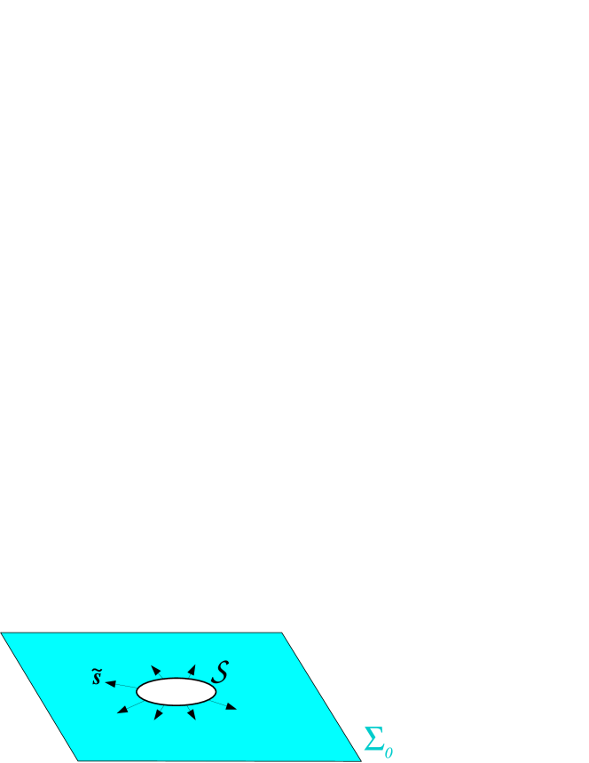
Figure 1: Hypersurface $\Sigma_{0}$ as $\mathbb{R}^{3}$ minus a ball, displayed via an embedding diagram based on the metric $\boldsymbol{{\tilde{\gamma}}}$, which coincides with the Euclidean metric on $\mathbb{R}^{3}$. Hence $\Sigma_{0}$ appears to be flat. The unit normal of the inner boundary $\mathcal{S}$ with respect to the metric $\boldsymbol{{\tilde{\gamma}}}$ is $\boldsymbol{\tilde{s}}$. Notice that $\boldsymbol{{\tilde{D}}}\cdot\boldsymbol{\tilde{s}}>0$.

4.2 Slice of Schwarzschild spacetime

To get something less trivial than a slice of Minkowski spacetime, let us consider a slightly more complicated topology for $\Sigma_{0}$, namely $\mathbb{R}^{3}$ minus a ball (cf. Fig. 1). The sphere $\mathcal{S}$ delimiting the ball is then the inner boundary of $\Sigma_{0}$ and we must provide boundary conditions for $\Psi$ and $\boldsymbol{X}$ on $\mathcal{S}$ to solve Eqs. (44)-(45). For simplicity, let us choose

$$\left.\boldsymbol{X}\right|_{\mathcal{S}}=0.$$ (54)

Altogether with the outer boundary condition (48), this leads to $\boldsymbol{X}$ being identically zero as the unique solution of Eq. (45). So, again, the Hamiltonian constraint reduces to Laplace equation

$$\Delta\Psi=0.$$ (55)

If we choose the boundary condition $\left.\Psi\right|_{\mathcal{S}}=1$, then the unique solution is $\Psi=1$ and we are back to the previous example (slice of Minkowski spacetime). In order to have something non trivial, i.e. to ensure that the metric $\boldsymbol{\gamma}$ will not be flat, let us demand that $\boldsymbol{\gamma}$ admits a closed minimal surface, that we will choose to be $\mathcal{S}$. This will necessarily translate as a boundary condition for $\Psi$ since all the information on the metric is encoded in $\Psi$ (let us recall that from the choice (40), $\boldsymbol{\gamma}=\Psi^{4}\boldsymbol{f}$). $\mathcal{S}$ is a minimal surface of $(\Sigma_{0},\boldsymbol{\gamma})$ iff its mean curvature vanishes, or equivalently if its unit normal $\boldsymbol{s}$ is divergence-free (cf. Fig. 2):

$$\left.D_{i}s^{i}\right|_{\mathcal{S}}=0.$$ (56)

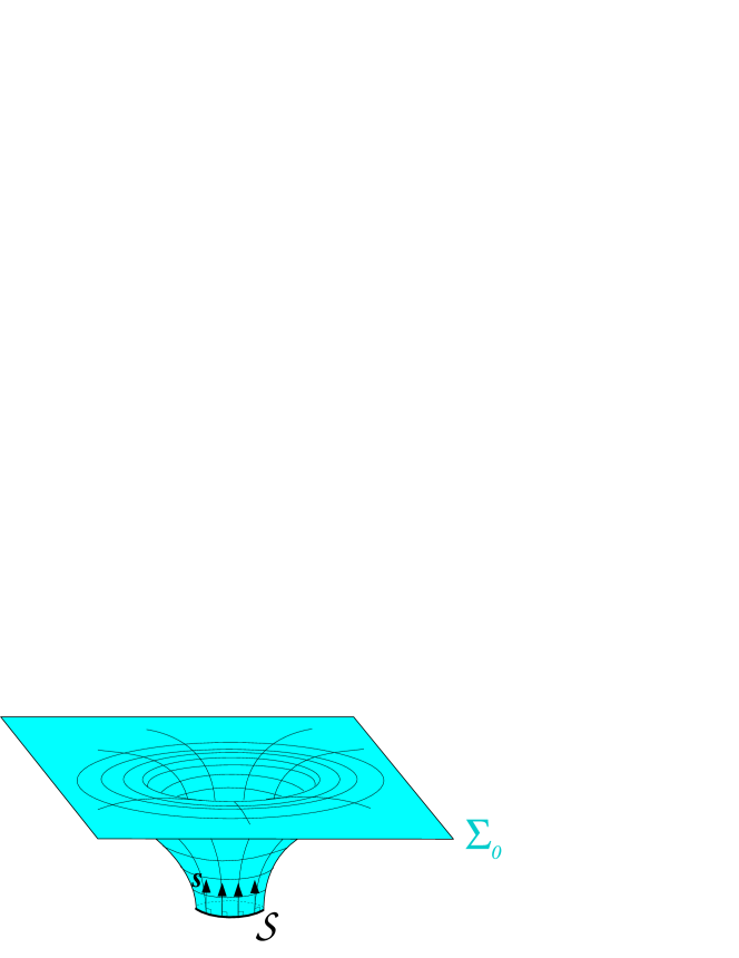
Figure 2: Same hypersurface $\Sigma_{0}$ as in Fig. 1 but displayed via an embedding diagram based on the metric $\boldsymbol{\gamma}$ instead of $\boldsymbol{{\tilde{\gamma}}}$. The unit normal of the inner boundary $\mathcal{S}$ with respect to that metric is $\boldsymbol{s}$. Notice that $\boldsymbol{D}\cdot\boldsymbol{s}=0$, which means that $\mathcal{S}$ is a minimal surface of $(\Sigma_{0},\boldsymbol{\gamma})$.

This is the analog of $\boldsymbol{\nabla}\cdot\boldsymbol{n}=0$ for maximal hypersurfaces, the change from minimal to maximal being due to the change of metric signature, from the Riemannian to the Lorentzian one. Expressed in term of the connection $\boldsymbol{{\tilde{D}}}=\boldsymbol{\mathcal{D}}$ (recall that in the present case $\boldsymbol{{\tilde{\gamma}}}=\boldsymbol{f}$), condition (56) is equivalent to

$$\left.\mathcal{D}_{i}(\Psi^{6}s^{i})\right|_{\mathcal{S}}=0.$$ (57)

Let us rewrite this expression in terms of the unit vector $\boldsymbol{\tilde{s}}$ normal to $\mathcal{S}$ with respect to the metric $\boldsymbol{{\tilde{\gamma}}}$ (cf. Fig. 1); we have

$$\boldsymbol{\tilde{s}}=\Psi^{-2}\boldsymbol{s},$$ (58)

since $\boldsymbol{{\tilde{\gamma}}}(\boldsymbol{\tilde{s}},\boldsymbol{\tilde{s}})=\Psi^{-4}\boldsymbol{{\tilde{\gamma}}}(\boldsymbol{s},\boldsymbol{s})=\boldsymbol{\gamma}(\boldsymbol{s},\boldsymbol{s})=1$. Thus Eq. (57) becomes

$$\left.\mathcal{D}_{i}(\Psi^{4}{\tilde{s}}^{i})\right|_{\mathcal{S}}=\left.\frac{1}{\sqrt{f}}\frac{\partial}{\partial x^{i}}\left(\sqrt{f}\Psi^{4}{\tilde{s}}^{i}\right)\right|_{\mathcal{S}}=0.$$ (59)

Let us introduce on $\Sigma_{0}$ a coordinate system of spherical type, $(x^{i})=(r,\theta,\varphi)$, such that (i) $f_{ij}=\mathrm{diag}(1,r^{2},r^{2}\sin^{2}\theta)$ and (ii) $\mathcal{S}$ is the sphere $r=a$, where $a$ is some positive constant. Since in these coordinates $\sqrt{f}=r^{2}\sin\theta$ and ${\tilde{s}}^{i}=(1,0,0)$, the minimal surface condition (59) is written as

$$\left.\frac{1}{r^{2}}\frac{\partial}{\partial r}\left(\Psi^{4}r^{2}\right)\right|_{r=a}=0,$$ (60)

i.e.

$$\left.\left(\frac{\partial\Psi}{\partial r}+\frac{\Psi}{2r}\right)\right|_{r=a}=0$$ (61)

This is a boundary condition of mixed Newmann/Dirichlet type for $\Psi$. The unique solution of the Laplace equation (55) which satisfies boundary conditions (47) and (61) is

$$\Psi=1+\frac{a}{r}.$$ (62)

The parameter $a$ is then easily related to the ADM mass $m$ of the hypersurface $\Sigma_{0}$. Indeed for a conformally flat 3-metric (and more generally in the quasi-isotropic gauge, cf. Chap. 7 of Ref. [51]), the ADM mass $m$ is given by the flux of the gradient of the conformal factor at spatial infinity:

$$m = -\frac{1}{2\pi}\lim_{r\rightarrow\infty}\oint_{r={\rm const}}\frac{\partial\Psi}{\partial r}r^{2}\sin\theta\,d\theta\,d\varphi$$ (63)

$$= -\frac{1}{2\pi}\lim_{r\rightarrow\infty}4\pi r^{2}\frac{\partial}{\partial r}\left(1+\frac{a}{r}\right)=2a.$$

Hence $a=m/2$ and we may write

$$\Psi=1+\frac{m}{2r}.$$ (64)

Therefore, in terms of the coordinates $(r,\theta,\varphi)$, the obtained initial data $(\boldsymbol{\gamma},\boldsymbol{K})$ are

$$\gamma_{ij}=\left(1+\frac{m}{2r}\right)^{4}\mathrm{diag}(1,r^{2},r^{2}\sin\theta)$$ (65)

$$K_{ij}=0.$$ (66)

So, as above, the initial data are momentarily static. Actually, we recognize on (65)-(66) a slice $t={\rm const}$ of Schwarzschild spacetime in isotropic coordinates.

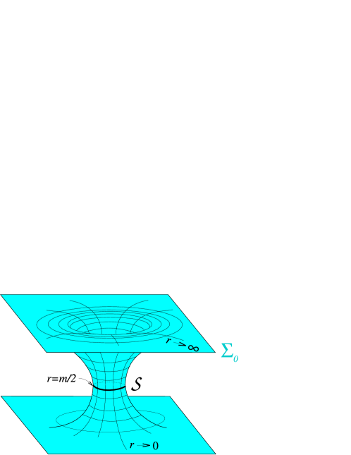
Figure 3: Extended hypersurface $\Sigma^{\prime}_{0}$ obtained by gluing a copy of $\Sigma_{0}$ at the minimal surface $\mathcal{S}$; it defines an Einstein-Rosen bridge between two asymptotically flat regions.

The isotropic coordinates $(r,\theta,\varphi)$ covering the manifold $\Sigma_{0}$ are such that the range of $r$ is $[m/2,+\infty)$. But thanks to the minimal character of the inner boundary $\mathcal{S}$, we can extend $(\Sigma_{0},\boldsymbol{\gamma})$ to a larger Riemannian manifold $(\Sigma^{\prime}_{0},\boldsymbol{\gamma}^{\prime})$ with $\left.\boldsymbol{\gamma}^{\prime}\right|_{\Sigma_{0}}=\boldsymbol{\gamma}$ and $\boldsymbol{\gamma}^{\prime}$ smooth at $\mathcal{S}$. This is made possible by gluing a copy of $\Sigma_{0}$ at $\mathcal{S}$ (cf. Fig. 3). The topology of $\Sigma^{\prime}_{0}$ is $\mathbb{S}^{2}\times\mathbb{R}$ and the range of $r$ in $\Sigma^{\prime}_{0}$ is $(0,+\infty)$. The extended metric $\boldsymbol{\gamma}^{\prime}$ keeps exactly the same form as (65):

$$\gamma^{\prime}_{ij}\,dx^{i}\,dx^{j}=\left(1+\frac{m}{2r}\right)^{4}\left(dr^{2}+r^{2}d\theta^{2}+r^{2}\sin^{2}\theta d\varphi^{2}\right).$$ (67)

By the change of variable

$$r\mapsto r^{\prime}=\frac{m^{2}}{4r}$$ (68)

it is easily shown that the region $r\rightarrow 0$ does not correspond to some “center” but is actually a second asymptotically flat region (the lower one in Fig. 3). Moreover the transformation (68), with $\theta$ and $\varphi$ kept fixed, is an isometry of $\boldsymbol{\gamma}^{\prime}$. It maps a point $p$ of $\Sigma_{0}$ to the point located at the vertical of $p$ in Fig. 3. The minimal sphere $\mathcal{S}$ is invariant under this isometry. The region around $\mathcal{S}$ is called an Einstein-Rosen bridge. $(\Sigma^{\prime}_{0},\boldsymbol{\gamma}^{\prime})$ is still a slice of Schwarzschild spacetime. It connects two asymptotically flat regions without entering below the event horizon, as shown in the Kruskal-Szekeres diagram of Fig. 4.

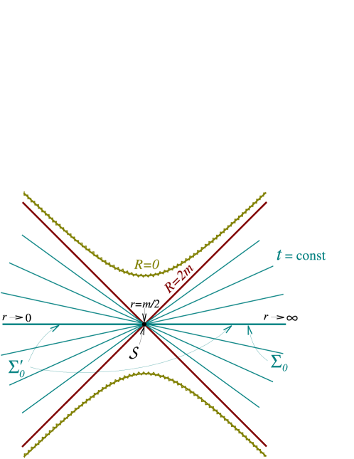
Figure 4: Extended hypersurface $\Sigma^{\prime}_{0}$ depicted in the Kruskal-Szekeres representation of Schwarzschild spacetime. $R$ stands for Schwarzschild radial coordinate and $r$ for the isotropic radial coordinate. $R=0$ is the singularity and $R=2m$ the event horizon. $\Sigma^{\prime}_{0}$ is nothing but a hypersurface $t={\rm const}$, where $t$ is the Schwarzschild time coordinate. In this diagram, these hypersurfaces are straight lines and the Einstein-Rosen bridge $\mathcal{S}$ is reduced to a point.

4.3 Bowen-York initial data

Let us select the same simple free data as above, namely

$${\tilde{\gamma}}_{ij}=f_{ij},\quad{\hat{A}}^{ij}_{\rm TT}=0,\quad K=0,\quad\tilde{E}=0\quad\mbox{and}\quad{\tilde{p}}^{i}=0.$$ (69)

For the hypersurface $\Sigma_{0}$, instead of $\mathbb{R}^{3}$ minus a ball, we choose $\mathbb{R}^{3}$ minus a point:

$$\Sigma_{0}=\mathbb{R}^{3}\backslash\{O\}.$$ (70)

The removed point $O$ is called a puncture [21]. The topology of $\Sigma_{0}$ is $\mathbb{S}^{2}\times\mathbb{R}$; it differs from the topology considered in Sec. 4.1 ($\mathbb{R}^{3}$ minus a ball); actually it is the same topology as that of the extended manifold $\Sigma^{\prime}_{0}$ (cf. Fig. 3).

Thanks to the choice (69), the system to be solved is still (44)-(45). If we choose the trivial solution $\boldsymbol{X}=0$ for Eq. (45), we are back to the slice of Schwarzschild spacetime considered in Sec. 4.1, except that now $\Sigma_{0}$ is the extended manifold previously denoted $\Sigma^{\prime}_{0}$.

Bowen and York [20] have obtained a simple non-trivial solution to the momentum constraint (45) (see also Ref. [15]). Given a Cartesian coordinate system $(x^{i})=(x,y,z)$ on $\Sigma_{0}$ (i.e. a coordinate system such that $f_{ij}=\mathrm{diag}(1,1,1)$) with respect to which the coordinates of the puncture $O$ are $(0,0,0)$, this solution writes

$$X^{i}=-\frac{1}{4r}\left(7f^{ij}P_{j}+\frac{P_{j}x^{j}x^{i}}{r^{2}}\right)-\frac{1}{r^{3}}\epsilon^{ij}_{\ \ k}S_{j}x^{k},$$ (71)

where $r:=\sqrt{x^{2}+y^{2}+z^{2}}$, $\epsilon^{ij}_{\ \ k}$ is the Levi-Civita alternating tensor associated with the flat metric $\boldsymbol{f}$ and $(P_{i},S_{j})=(P_{1},P_{2},P_{3},S_{1},S_{2},S_{3})$ are six real numbers, which constitute the six parameters of the Bowen-York solution. Notice that since $r\not=0$ on $\Sigma_{0}$, the Bowen-York solution is a regular and smooth solution on the entire $\Sigma_{0}$.

The conformal traceless extrinsic curvature corresponding to the solution (71) is deduced from formula (13), which in the present case reduces to ${\hat{A}}^{ij}=(LX)^{ij}$; one gets

$${\hat{A}}^{ij}=\frac{3}{2r^{3}}\left[x^{i}P^{j}+x^{j}P^{i}-\left(f^{ij}-\frac{x^{i}x^{j}}{r^{2}}\right)P_{k}x^{k}\right]+\frac{3}{r^{5}}\left(\epsilon^{ik}_{\ \ l}S_{k}x^{l}x^{j}+\epsilon^{jk}_{\ \ l}S_{k}x^{l}x^{i}\right),$$ (72)

where $P^{i}:=f^{ij}P_{j}$. The tensor ${\hat{A}}^{ij}$ given by Eq. (72) is called the Bowen-York extrinsic curvature. Notice that the $P_{i}$ part of ${\hat{A}}^{ij}$ decays asymptotically as $O(r^{-2})$, whereas the $S_{i}$ part decays as $O(r^{-3})$.

Remark :

Actually the expression of ${\hat{A}}^{ij}$ given in the original Bowen-York article [20] contains an additional term with respect to Eq. (72), but the role of this extra term is only to ensure that the solution is isometric through an inversion across some sphere. We are not interested by such a property here, so we have dropped this term. Therefore, strictly speaking, we should name expression (72) the simplified Bowen-York extrinsic curvature.

The Bowen-York extrinsic curvature provides an analytical solution of the momentum constraint (45) but there remains to solve the Hamiltonian constraint (44) for $\Psi$, with the asymptotic flatness boundary condition $\Psi=1$ when $r\rightarrow\infty$. Since $\boldsymbol{X}\not=0$, Eq. (44) is no longer a simple Laplace equation, as in Sec. 4.1, but a non-linear elliptic equation. There is no hope to get any analytical solution and one must solve Eq. (44) numerically to get $\Psi$ and reconstruct the full initial data $(\boldsymbol{\gamma},\boldsymbol{K})$ via Eqs. (29)-(30).

The parameters $P_{i}$ of the Bowen-York solution are nothing but the three components of the ADM linear momentum of the hypersurface $\Sigma_{0}$ Similarly, the parameters $S_{i}$ of the Bowen-York solution are nothing but the three components of the angular momentum of the hypersurface $\Sigma_{0}$, the latter being defined relatively to the quasi-isotropic gauge, in the absence of any axial symmetry (see e.g. [51]).

Remark :

The Bowen-York solution with $P^{i}=0$ and $S^{i}=0$ reduces to the momentarily static solution found in Sec. 4.1, i.e. is a slice $t={\rm const}$ of the Schwarzschild spacetime ($t$ being the Schwarzschild time coordinate). However Bowen-York initial data with $P^{i}=0$ and $S^{i}\not=0$ do not constitute a slice of Kerr spacetime. Indeed, it has been shown [47] that there does not exist any foliation of Kerr spacetime by hypersurfaces which (i) are axisymmetric, (ii) smoothly reduce in the non-rotating limit to the hypersurfaces of constant Schwarzschild time and (iii) are conformally flat, i.e. have induced metric $\boldsymbol{{\tilde{\gamma}}}=\boldsymbol{f}$, as the Bowen-York hypersurfaces have. This means that a Bowen-York solution with $S^{i}\not=0$ does represent initial data for a rotating black hole, but this black hole is not stationary: it is “surrounded” by gravitational radiation, as demonstrated by the time development of these initial data [22, 49].

5 Conformal thin sandwich method

5.1 The original conformal thin sandwich method

An alternative to the conformal transverse-traceless method for computing initial data has been introduced by York in 1999 [107]. The starting point is the identity

$$\boldsymbol{K}=-\frac{1}{2N}\boldsymbol{\mathcal{L}}_{N\boldsymbol{n}}\boldsymbol{\gamma}=-\frac{1}{2N}\left(\frac{\partial}{\partial t}-\boldsymbol{\mathcal{L}}_{\boldsymbol{\beta}}\,\right)\boldsymbol{\gamma},$$ (73)

where $N$ is the lapse function and $\boldsymbol{\beta}$ is the shift vector associated with some 3+1 coordinates $(t,x^{i})$. The traceless part of Eq. (73) leads to

$${\tilde{A}}^{ij}=\frac{1}{2N}\left[\left(\frac{\partial}{\partial t}-{\mathcal{L}}_{\boldsymbol{\beta}}\,\right){\tilde{\gamma}}^{ij}-\frac{2}{3}{\tilde{D}}_{k}\beta^{k}\,{\tilde{\gamma}}^{ij}\right],$$ (74)

where ${\tilde{A}}^{ij}$ is defined by Eq. (8). Noticing that

$$-{\mathcal{L}}_{\boldsymbol{\beta}}\,{\tilde{\gamma}}^{ij}=(\tilde{L}\beta)^{ij}+\frac{2}{3}{\tilde{D}}_{k}\beta^{k},$$ (75)

and introducing the short-hand notation

$$\dot{\tilde{\gamma}}^{ij}:=\frac{\partial}{\partial t}{\tilde{\gamma}}^{ij},$$ (76)

we can rewrite Eq. (74) as

$${\tilde{A}}^{ij}=\frac{1}{2N}\left[\dot{\tilde{\gamma}}^{ij}+(\tilde{L}\beta)^{ij}\right].$$ (77)

The relation between ${\tilde{A}}^{ij}$ and ${\hat{A}}^{ij}$ is [cf. Eqs. (7)-(8)]

$${\hat{A}}^{ij}=\Psi^{6}{\tilde{A}}^{ij}.$$ (78)

Accordingly, Eq. (77) yields

$${\hat{A}}^{ij}=\frac{1}{2\tilde{N}}\left[\dot{\tilde{\gamma}}^{ij}+(\tilde{L}\beta)^{ij}\right],$$ (79)

where we have introduced the conformal lapse

$$\tilde{N}:=\Psi^{-6}N.$$ (80)

Equation (79) constitutes a decomposition of ${\hat{A}}^{ij}$ alternative to the longitudinal/transverse decomposition (13). Instead of expressing ${\hat{A}}^{ij}$ in terms of a vector $\boldsymbol{X}$ and a TT tensor ${\hat{A}}^{ij}_{\rm TT}$, it expresses it in terms of the shift vector $\boldsymbol{\beta}$, the time derivative of the conformal metric, $\dot{\tilde{\gamma}}^{ij}$, and the conformal lapse $\tilde{N}$.

The Hamiltonian constraint, written as the Lichnerowicz equation (10), takes the same form as before:

$${\tilde{D}}_{i}{\tilde{D}}^{i}\Psi-\frac{{\tilde{R}}}{8}\Psi+\frac{1}{8}{\hat{A}}_{ij}{\hat{A}}^{ij}\,\Psi^{-7}+2\pi{\tilde{E}}\Psi^{-3}-\frac{K^{2}}{12}\Psi^{5}=0,$$ (81)

except that now ${\hat{A}}^{ij}$ is to be understood as the combination (79) of $\beta^{i}$, $\dot{\tilde{\gamma}}^{ij}$ and $\tilde{N}$. On the other side, the momentum constraint (11) becomes, once expression (79) is substituted for ${\hat{A}}^{ij}$,

$${\tilde{D}}_{j}\left(\frac{1}{\tilde{N}}(\tilde{L}\beta)^{ij}\right)+{\tilde{D}}_{j}\left(\frac{1}{\tilde{N}}\dot{\tilde{\gamma}}^{ij}\right)-\frac{4}{3}\Psi^{6}{\tilde{D}}^{i}K=16\pi{\tilde{p}}^{i}.$$ (82)

In view of the system (81)-(82), the method to compute initial data consists in choosing freely ${\tilde{\gamma}}_{ij}$, $\dot{\tilde{\gamma}}^{ij}$, $K$, ${\tilde{N}}$, ${\tilde{E}}$ and ${\tilde{p}}^{i}$ on $\Sigma_{0}$ and solving (81)-(82) to get $\Psi$ and $\beta^{i}$. This method is called conformal thin sandwich (CTS), because one input is the time derivative $\dot{\tilde{\gamma}}^{ij}$, which can be obtained from the value of the conformal metric on two neighbouring hypersurfaces $\Sigma_{t}$ and $\Sigma_{t+\delta t}$ (“thin sandwich” view point).

Remark :

The term “thin sandwich” originates from a previous method devised in the early sixties by Wheeler and his collaborators [4, 101]. Contrary to the methods exposed here, the thin sandwich method was not based on a conformal decomposition: it considered the constraint equations (1)-(2) as a system to be solved for the lapse $N$ and the shift vector $\boldsymbol{\beta}$, given the metric $\boldsymbol{\gamma}$ and its time derivative. The extrinsic curvature which appears in (1)-(2) was then considered as the function of $\boldsymbol{\gamma}$, ${\partial\boldsymbol{\gamma}}/{\partial t}$, $N$ and $\boldsymbol{\beta}$ given by Eq. (73). However, this method does not work in general [9]. On the contrary the conformal thin sandwich method introduced by York [107] and exposed above was shown to work [35].

As for the conformal transverse-traceless method treated in Sec. 3, on CMC hypersurfaces, Eq. (82) decouples from Eq. (81) and becomes an elliptic linear equation for $\boldsymbol{\beta}$.

5.2 Extended conformal thin sandwich method

An input of the above method is the conformal lapse $\tilde{N}$. Considering the astrophysical problem stated in Sec. 2.2, it is not clear how to pick a relevant value for $\tilde{N}$. Instead of choosing an arbitrary value, Pfeiffer and York [80] have suggested to compute $\tilde{N}$ from the Einstein equation giving the time derivative of the trace $K$ of the extrinsic curvature, i.e.

$$\left(\frac{\partial}{\partial t}-{\mathcal{L}}_{\boldsymbol{\beta}}\,\right)K = -\Psi^{-4}\left({\tilde{D}}_{i}{\tilde{D}}^{i}N+2{\tilde{D}}_{i}\ln\Psi\,{\tilde{D}}^{i}N\right)$$ (83)

$$+N\left[4\pi(E+S)+{\tilde{A}}_{ij}{\tilde{A}}^{ij}+\frac{K^{2}}{3}\right],$$

where $S$ is the trace of the matter stress tensor as measured by the Eulerian observer: $S=\gamma^{\mu\nu}T_{\mu\nu}$. This amounts to add this equation to the initial data system. More precisely, Pfeiffer and York [80] suggested to combine Eq. (83) with the Hamiltonian constraint to get an equation involving the quantity $N\Psi=\tilde{N}\Psi^{7}$ and containing no scalar products of gradients as the ${\tilde{D}}_{i}\ln\Psi{\tilde{D}}^{i}N$ term in Eq. (83), thanks to the identity

$${\tilde{D}}_{i}{\tilde{D}}^{i}N+2{\tilde{D}}_{i}\ln\Psi\,{\tilde{D}}^{i}N=\Psi^{-1}\left[{\tilde{D}}_{i}{\tilde{D}}^{i}(N\Psi)+N{\tilde{D}}_{i}{\tilde{D}}^{i}\Psi\right].$$ (84)

Expressing the left-hand side of the above equation in terms of Eq. (83) and substituting ${\tilde{D}}_{i}{\tilde{D}}^{i}\Psi$ in the right-hand side by its expression deduced from Eq. (81), we get

$${\tilde{D}}_{i}{\tilde{D}}^{i}(\tilde{N}\Psi^{7})-(\tilde{N}\Psi^{7})\left[\frac{1}{8}\tilde{R}+\frac{5}{12}K^{2}\Psi^{4}+\frac{7}{8}{\hat{A}}_{ij}{\hat{A}}^{ij}\Psi^{-8}+2\pi(\tilde{E}+2\tilde{S})\Psi^{-4}\right]$$

$$+\left(\dot{K}-\beta^{i}{\tilde{D}}_{i}K\right)\Psi^{5}=0,$$ (85)

where we have used the short-hand notation

$$\dot{K}:=\frac{\partial K}{\partial t}$$ (86)

and have set

$$\tilde{S}:=\Psi^{8}S.$$ (87)

Adding Eq. (85) to Eqs. (81) and (82), the initial data system becomes

$${\tilde{D}}_{i}{\tilde{D}}^{i}\Psi-\frac{{\tilde{R}}}{8}\Psi+\frac{1}{8}{\hat{A}}_{ij}{\hat{A}}^{ij}\,\Psi^{-7}+2\pi{\tilde{E}}\Psi^{-3}-\frac{K^{2}}{12}\Psi^{5}=0$$ (88)

$${\tilde{D}}_{j}\left(\frac{1}{\tilde{N}}(\tilde{L}\beta)^{ij}\right)+{\tilde{D}}_{j}\left(\frac{1}{\tilde{N}}\dot{\tilde{\gamma}}^{ij}\right)-\frac{4}{3}\Psi^{6}{\tilde{D}}^{i}K=16\pi{\tilde{p}}^{i}$$ (89)

$${\tilde{D}}_{i}{\tilde{D}}^{i}(\tilde{N}\Psi^{7})-(\tilde{N}\Psi^{7})\bigg{[}\frac{\tilde{R}}{8}+\frac{5}{12}K^{2}\Psi^{4}+\frac{7}{8}{\hat{A}}_{ij}{\hat{A}}^{ij}\Psi^{-8}+2\pi(\tilde{E}+2\tilde{S})\Psi^{-4}\bigg{]}$$

$$+\left(\dot{K}-\beta^{i}{\tilde{D}}_{i}K\right)\Psi^{5}=0,$$ (90)

where ${\hat{A}}^{ij}$ is the function of $\tilde{N}$, $\beta^{i}$, ${\tilde{\gamma}}_{ij}$ and $\dot{\tilde{\gamma}}^{ij}$ defined by Eq. (79). Equations (88)-(90) constitute the extended conformal thin sandwich (XCTS) system for the initial data problem. The free data are the conformal metric $\boldsymbol{{\tilde{\gamma}}}$, its coordinate time derivative $\boldsymbol{\dot{\tilde{\gamma}}}$, the extrinsic curvature trace $K$, its coordinate time derivative $\dot{K}$, and the rescaled matter variables $\tilde{E}$, $\tilde{S}$ and $\tilde{p}^{i}$. The constrained data are the conformal factor $\Psi$, the conformal lapse $\tilde{N}$ and the shift vector $\boldsymbol{\beta}$.

Remark :

The XCTS system (88)-(90) is a coupled system. Contrary to the CTT system (26)-(27), the assumption of constant mean curvature, and in particular of maximal slicing, does not allow to decouple it.

5.3 XCTS at work: static black hole example

Let us illustrate the extended conformal thin sandwich method on a simple example. Take for the hypersurface $\Sigma_{0}$ the punctured manifold considered in Sec. 4.3, namely

$$\Sigma_{0}=\mathbb{R}^{3}\backslash\{O\}.$$ (91)

For the free data, let us perform the simplest choice:

$${\tilde{\gamma}}_{ij}=f_{ij},\quad\dot{\tilde{\gamma}}^{ij}=0,\quad K=0,\quad\dot{K}=0,\quad\tilde{E}=0,\quad\tilde{S}=0,\quad\mbox{and}\quad{\tilde{p}}^{i}=0,$$ (92)

i.e. we are searching for vacuum initial data on a maximal and conformally flat hypersurface with all the freely specifiable time derivatives set to zero. Thanks to (92), the XCTS system (88)-(90) reduces to

$$\Delta\Psi+\frac{1}{8}{\hat{A}}_{ij}{\hat{A}}^{ij}\,\Psi^{-7}=0$$ (93)

$$\mathcal{D}_{j}\left(\frac{1}{\tilde{N}}(L\beta)^{ij}\right)=0$$ (94)

$$\Delta(\tilde{N}\Psi^{7})-\frac{7}{8}{\hat{A}}_{ij}{\hat{A}}^{ij}\Psi^{-1}\tilde{N}=0.$$ (95)

Aiming at finding the simplest solution, we notice that

$$\boldsymbol{\beta}=0$$ (96)

is a solution of Eq. (94). Together with $\dot{\tilde{\gamma}}^{ij}=0$, it leads to [cf. Eq. (79)]

$${\hat{A}}^{ij}=0.$$ (97)

The system (93)-(95) reduces then further:

$$\Delta\Psi=0$$ (98)

$$\Delta(\tilde{N}\Psi^{7})=0.$$ (99)

Hence we have only two Laplace equations to solve. Moreover Eq. (98) decouples from Eq. (99). For simplicity, let us assume spherical symmetry around the puncture $O$. We introduce an adapted spherical coordinate system $(x^{i})=(r,\theta,\varphi)$ on $\Sigma_{0}$. The puncture $O$ is then at $r=0$. The simplest non-trivial solution of (98) which obeys the asymptotic flatness condition $\Psi\rightarrow 1$ as $r\rightarrow+\infty$ is

$$\Psi=1+\frac{m}{2r},$$ (100)

where as in Sec. 4.1, the constant $m$ is the ADM mass of $\Sigma_{0}$ [cf. Eq. (63)]. Notice that since $r=0$ is excluded from $\Sigma_{0}$, $\Psi$ is a perfectly regular solution on the entire manifold $\Sigma_{0}$. Let us recall that the Riemannian manifold $(\Sigma_{0},\boldsymbol{\gamma})$ corresponding to this value of $\Psi$ via $\boldsymbol{\gamma}=\Psi^{4}\boldsymbol{f}$ is the Riemannian manifold denoted $(\Sigma^{\prime}_{0},\boldsymbol{\gamma})$ in Sec. 4.1 and depicted in Fig. 3. In particular it has two asymptotically flat ends: $r\rightarrow+\infty$ and $r\rightarrow 0$ (the puncture).

As for Eq. (98), the simplest solution of Eq. (99) obeying the asymptotic flatness requirement $\tilde{N}\Psi^{7}\rightarrow 1$ as $r\rightarrow+\infty$ is

$$\tilde{N}\Psi^{7}=1+\frac{a}{r},$$ (101)

where $a$ is some constant. Let us determine $a$ from the value of the lapse function at the second asymptotically flat end $r\rightarrow 0$. The lapse being related to $\tilde{N}$ via Eq. (80), Eq. (101) is equivalent to

$$N=\left(1+\frac{a}{r}\right)\Psi^{-1}=\left(1+\frac{a}{r}\right)\left(1+\frac{m}{2r}\right)^{-1}=\frac{r+a}{r+m/2}.$$ (102)

Hence

$$\lim_{r\rightarrow 0}N=\frac{2a}{m}.$$ (103)

There are two natural choices for $\lim_{r\rightarrow 0}N$. The first one is

$$\lim_{r\rightarrow 0}N=1,$$ (104)

yielding $a=m/2$. Then, from Eq. (102) $N=1$ everywhere on $\Sigma_{0}$. This value of $N$ corresponds to a geodesic slicing. The second choice is

$$\lim_{r\rightarrow 0}N=-1.$$ (105)

This choice is compatible with asymptotic flatness: it simply means that the coordinate time $t$ is running “backward” near the asymptotic flat end $r\rightarrow 0$. This contradicts the assumption $N>0$ in the standard definition of the lapse function. However, we shall generalize here the definition of the lapse to allow for negative values: whereas the unit vector $\boldsymbol{n}$ is always future-oriented, the scalar field $t$ is allowed to decrease towards the future. Such a situation has already been encountered for the part of the slices $t={\rm const}$ located on the left side of Fig. 4. Once reported into Eq. (103), the choice (105) yields $a=-m/2$, so that

$$N=\left(1-\frac{m}{2r}\right)\left(1+\frac{m}{2r}\right)^{-1}.$$ (106)

Gathering relations (96), (100) and (106), we arrive at the following expression of the spacetime metric components:

$$g_{\mu\nu}dx^{\mu}dx^{\nu}=-\left(\frac{1-\frac{m}{2r}}{1+\frac{m}{2r}}\right)^{2}dt^{2}+\left(1+\frac{m}{2r}\right)^{4}\left[d{r}^{2}+{r}^{2}(d\theta^{2}+\sin^{2}\theta d\varphi^{2})\right].$$ (107)

We recognize the line element of Schwarzschild spacetime in isotropic coordinates. Hence we recover the same initial data as in Sec. 4.1 and depicted in Figs. 3 and 4. The bonus is that we have the complete expression of the metric $\boldsymbol{g}$ on $\Sigma_{0}$, and not only the induced metric $\boldsymbol{\gamma}$.

Remark :

The choices (104) and (105) for the asymptotic value of the lapse both lead to a momentarily static initial slice in Schwarzschild spacetime. The difference is that the time development corresponding to choice (104) (geodesic slicing) will depend on $t$, whereas the time development corresponding to choice (105) will not, since in the latter case $t$ coincides with the standard Schwarzschild time coordinate, which makes $\boldsymbol{\partial}_{t}$ a Killing vector.

5.4 Uniqueness of solutions

Recently, Pfeiffer and York [81] have exhibited a choice of vacuum free data $({\tilde{\gamma}}_{ij},\dot{\tilde{\gamma}}^{ij},K,\dot{K})$ for which the solution $(\Psi,\tilde{N},\beta^{i})$ to the XCTS system (88)-(90) is not unique (actually two solutions are found). The conformal metric $\boldsymbol{{\tilde{\gamma}}}$ is the flat metric plus a linearized quadrupolar gravitational wave, as obtained by Teukolsky [92], with a tunable amplitude. $\dot{\tilde{\gamma}}^{ij}$ corresponds to the time derivative of this wave, and both $K$ and $\dot{K}$ are chosen to zero. On the contrary, for the same free data, with $\dot{K}=0$ substituted by $\tilde{N}=1$, Pfeiffer and York have shown that the original conformal thin sandwich method as described in Sec. 5.1 leads to a unique solution (or no solution at all if the amplitude of the wave is two large).

Baumgarte, Ó Murchadha and Pfeiffer [14] have argued that the lack of uniqueness for the XCTS system may be due to the term

$$-(\tilde{N}\Psi^{7})\frac{7}{8}{\hat{A}}_{ij}{\hat{A}}^{ij}\Psi^{-8}=-\frac{7}{32}\Psi^{6}{\tilde{\gamma}}_{ik}{\tilde{\gamma}}_{jl}\left[\dot{\tilde{\gamma}}^{ij}+(\tilde{L}\beta)^{ij}\right]\left[\dot{\tilde{\gamma}}^{kl}+(\tilde{L}\beta)^{kl}\right]\,(\tilde{N}\Psi^{7})^{-1}$$ (108)

in Eq. (90). Indeed, if we proceed as for the analysis of Lichnerowicz equation in Sec. 3.4, we notice that this term, with the minus sign and the negative power of $(\tilde{N}\Psi^{7})^{-1}$, makes the linearization of Eq. (90) of the type ${\tilde{D}}_{i}{\tilde{D}}^{i}\epsilon+\alpha\epsilon=\sigma$, with $\alpha>0$. This “wrong” sign of $\alpha$ prevents the application of the maximum principle to guarantee the uniqueness of the solution.

The non-uniqueness of solution of the XCTS system for certain choice of free data has been confirmed by Walsh [100] by means of bifurcation theory.

5.5 Comparing CTT, CTS and XCTS

The conformal transverse traceless (CTT) method exposed in Sec. 3 and the (extended) conformal thin sandwich (XCTS) method considered here differ by the choice of free data: whereas both methods use the conformal metric $\boldsymbol{{\tilde{\gamma}}}$ and the trace of the extrinsic curvature $K$ as free data, CTT employs in addition ${\hat{A}}^{ij}_{\rm TT}$, whereas for CTS (resp. XCTS) the additional free data is $\dot{\tilde{\gamma}}^{ij}$, as well as $\tilde{N}$ (resp. $\dot{K}$). Since ${\hat{A}}^{ij}_{\rm TT}$ is directly related to the extrinsic curvature and the latter is linked to the canonical momentum of the gravitational field in the Hamiltonian formulation of general relativity, the CTT method can be considered as the approach to the initial data problem in the Hamiltonian representation. On the other side, $\dot{\tilde{\gamma}}^{ij}$ being the “velocity” of ${\tilde{\gamma}}^{ij}$, the (X)CTS method constitutes the approach in the Lagrangian representation [108].

Remark :

The (X)CTS method assumes that the conformal metric is unimodular: $\det({\tilde{\gamma}}_{ij})=f$ (since Eq. (79) follows from this assumption), whereas the CTT method can be applied with any conformal metric.

The advantage of CTT is that its mathematical theory is well developed, yielding existence and uniqueness theorems, at least for constant mean curvature (CMC) slices. The mathematical theory of CTS is very close to CTT. In particular, the momentum constraint decouples from the Hamiltonian constraint on CMC slices. On the contrary, XCTS has a much more involved mathematical structure. In particular the CMC condition does not yield to any decoupling. The advantage of XCTS is then to be better suited to the description of quasi-stationary spacetimes, since $\dot{\tilde{\gamma}}^{ij}=0$ and $\dot{K}=0$ are necessary conditions for $\boldsymbol{\partial}_{t}$ to be a Killing vector. This makes XCTS the method to be used in order to prepare initial data in quasi-equilibrium. For instance, it has been shown [57, 43] that XCTS yields orbiting binary black hole configurations in much better agreement with post-Newtonian computations than the CTT treatment based on a superposition of two Bowen-York solutions. Indeed, except when they are very close and about to merge, the orbits of binary black holes evolve very slowly, so that it is a very good approximation to consider that the system is in quasi-equilibrium. XCTS takes this fully into account, while CTT relies on a technical simplification (Bowen-York analytical solution of the momentum constraint), with no direct relation to the quasi-equilibrium state.

A detailed comparison of CTT and XCTS for a single spinning or boosted black hole has been performed by Laguna [68].

6 Initial data for binary systems

A major topic of contemporary numerical relativity is the computation of the merger of a binary system of black holes [24] or neutron stars [84], for such systems are among the most promising sources of gravitational radiation for the interferometric detectors either groundbased (LIGO, VIRGO, GEO600, TAMA) or in space (LISA). The problem of preparing initial data for these systems has therefore received a lot of attention in the past decade.

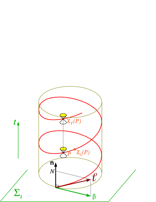
Figure 5: Action of the helical symmetry group, with Killing vector $\boldsymbol{\ell}$. $\chi_{\tau}(P)$ is the displacement of the point $P$ by the member of the symmetry group of parameter $\tau$. $N$ and $\boldsymbol{\beta}$ are respectively the lapse function and the shift vector associated with coordinates adapted to the symmetry, i.e. coordinates $(t,x^{i})$ such that $\boldsymbol{\partial}_{t}=\boldsymbol{\ell}$.

6.1 Helical symmetry

Due to the gravitational-radiation reaction, a relativistic binary system has an inspiral motion, leading to the merger of the two components. However, when the two bodies are sufficiently far apart, one may approximate the spiraling orbits by closed ones. Moreover, it is well known that gravitational radiation circularizes the orbits very efficiently, at least for comparable mass systems [18]. We may then consider that the motion is described by a sequence of closed circular orbits.

The geometrical translation of this physical assumption is that the spacetime $(\mathcal{M},\boldsymbol{g})$ is endowed with some symmetry, called helical symmetry. Indeed exactly circular orbits imply the existence of a one-parameter symmetry group such that the associated Killing vector $\boldsymbol{\ell}$ obeys the following properties [46]: (i) $\boldsymbol{\ell}$ is timelike near the system, (ii) far from it, $\boldsymbol{\ell}$ is spacelike but there exists a smaller number $T>0$ such that the separation between any point $P$ and its image $\chi_{T}(P)$ under the symmetry group is timelike (cf. Fig. 5). $\boldsymbol{\ell}$ is called a helical Killing vector, its field lines in a spacetime diagram being helices (cf. Fig. 5).

Helical symmetry is exact in theories of gravity where gravitational radiation does not exist, namely:

• in Newtonian gravity,

• in post-Newtonian gravity, up to the second order,

• in the Isenberg-Wilson-Mathews (IWM) approximation to general relativity, based on the assumptions $\boldsymbol{{\tilde{\gamma}}}=\boldsymbol{f}$ and $K=0$ [61, 102].

Moreover helical symmetry can be exact in full general relativity for a non-axisymmetric system (such as a binary) with standing gravitational waves [44]. But notice that a spacetime with helical symmetry and standing gravitational waves cannot be asymptotically flat [48].

To treat helically symmetric spacetimes, it is natural to choose coordinates $(t,x^{i})$ that are adapted to the symmetry, i.e. such that

$$\boldsymbol{\partial}_{t}=\boldsymbol{\ell}.$$ (109)

Then all the fields are independent of the coordinate $t$. In particular,

$$\dot{\tilde{\gamma}}^{ij}=0\qquad\mbox{and}\qquad\dot{K}=0.$$ (110)

If we employ the XCTS formalism to compute initial data, we therefore get some definite prescription for the free data $\dot{\tilde{\gamma}}^{ij}$ and $\dot{K}$. On the contrary, the requirements (110) do not have any immediate translation in the CTT formalism.

Remark :

Helical symmetry can also be useful to treat binary black holes outside the scope of the 3+1 formalism, as shown by Klein [67], who developed a quotient space formalism to reduce the problem to a three dimensional $\mathrm{SL}(2,\mathbb{R})/\mathrm{SO}(1,1)$ sigma model.

Taking into account (110) and choosing maximal slicing ($K=0$), the XCTS system (88)-(90) becomes

$${\tilde{D}}_{i}{\tilde{D}}^{i}\Psi-\frac{{\tilde{R}}}{8}\Psi+\frac{1}{8}{\hat{A}}_{ij}{\hat{A}}^{ij}\,\Psi^{-7}+2\pi{\tilde{E}}\Psi^{-3}=0$$ (111)

$${\tilde{D}}_{j}\left(\frac{1}{\tilde{N}}(\tilde{L}\beta)^{ij}\right)-16\pi{\tilde{p}}^{i}=0$$ (112)

$${\tilde{D}}_{i}{\tilde{D}}^{i}(\tilde{N}\Psi^{7})-(\tilde{N}\Psi^{7})\left[\frac{\tilde{R}}{8}+\frac{7}{8}{\hat{A}}_{ij}{\hat{A}}^{ij}\Psi^{-8}+2\pi(\tilde{E}+2\tilde{S})\Psi^{-4}\right]=0,$$ (113)

where [cf. Eq. (79)]

$${\hat{A}}^{ij}=\frac{1}{2\tilde{N}}(\tilde{L}\beta)^{ij}.$$ (114)

6.2 Helical symmetry and IWM approximation

If we choose, as part of the free data, the conformal metric to be flat,

$${\tilde{\gamma}}_{ij}=f_{ij},$$ (115)

then the helically symmetric XCTS system (111)-(113) reduces to

$$\Delta\Psi+\frac{1}{8}{\hat{A}}_{ij}{\hat{A}}^{ij}\,\Psi^{-7}+2\pi{\tilde{E}}\Psi^{-3}=0$$ (116)

$$\Delta\beta^{i}+\frac{1}{3}\mathcal{D}^{i}\mathcal{D}_{j}\beta^{j}-(L\beta)^{ij}\mathcal{D}_{j}\ln\tilde{N}=16\pi{\tilde{N}}{\tilde{p}}^{i}$$ (117)

$$\Delta(\tilde{N}\Psi^{7})-(\tilde{N}\Psi^{7})\left[\frac{7}{8}{\hat{A}}_{ij}{\hat{A}}^{ij}\Psi^{-8}+2\pi(\tilde{E}+2\tilde{S})\Psi^{-4}\right]=0,$$ (118)

where

$${\hat{A}}^{ij}=\frac{1}{2\tilde{N}}(L\beta)^{ij}$$ (119)

and $\boldsymbol{\mathcal{D}}$ is the connection associated with the flat metric $\boldsymbol{f}$, $\Delta:=\mathcal{D}_{i}\mathcal{D}^{i}$ is the flat Laplacian [Eq. (46)], and $(L\beta)^{ij}:=\mathcal{D}^{i}\beta^{j}+\mathcal{D}^{j}\beta^{i}-\frac{2}{3}\mathcal{D}_{k}\beta^{k}\,f^{ij}$ [Eq. (15) with ${\tilde{D}}^{i}=\mathcal{D}^{i}$].

We remark that the system (116)-(118) is identical to the system defining the Isenberg-Wilson-Mathews approximation to general relativity [61, 102] (see e.g. Sec. 6.6 of Ref. [51]). This means that, within helical symmetry, the XCTS system with the choice $K=0$ and $\boldsymbol{{\tilde{\gamma}}}=\boldsymbol{f}$ is equivalent to the IWM system.

Remark :

Contrary to IWM, XCTS is not some approximation to general relativity: it provides exact initial data. The only thing that may be questioned is the astrophysical relevance of the XCTS data with $\boldsymbol{{\tilde{\gamma}}}=\boldsymbol{f}$.

6.3 Initial data for orbiting binary black holes

The concept of helical symmetry for generating orbiting binary black hole initial data has been introduced in 2002 by Gourgoulhon, Grandclément and Bonazzola [52, 57]. The system of equations that these authors have derived is equivalent to the XCTS system with $\boldsymbol{{\tilde{\gamma}}}=\boldsymbol{f}$, their work being previous to the formulation of the XCTS method by Pfeiffer and York (2003) [80]. Since then other groups have combined XCTS with helical symmetry to compute binary black hole initial data [38, 1, 2, 31]. Since all these studies are using a flat conformal metric [choice (115)], the PDE system to be solved is (116)-(118), with the additional simplification $\tilde{E}=0$ and ${\tilde{p}}^{i}=0$ (vacuum). The initial data manifold $\Sigma_{0}$ is chosen to be $\mathbb{R}^{3}$ minus two balls:

$$\Sigma_{0}=\mathbb{R}^{3}\backslash(\mathcal{B}_{1}\cup\mathcal{B}_{2}).$$ (120)

In addition to the asymptotic flatness conditions, some boundary conditions must be provided on the surfaces $\mathcal{S}_{1}$ and $\mathcal{S}_{2}$ of $\mathcal{B}_{1}$ and $\mathcal{B}_{2}$. One choose boundary conditions corresponding to a non-expanding horizon, since this concept characterizes black holes in equilibrium. We shall not detail these boundary conditions here; they can be found in Refs. [38, 40, 41, 54, 65]. The condition of non-expanding horizon provides 3 among the 5 required boundary conditions [for the 5 components $(\Psi,\tilde{N},\beta^{i})$]. The two remaining boundary conditions are given by (i) the choice of the foliation (choice of the value of $N$ at $\mathcal{S}_{1}$ and $\mathcal{S}_{2}$) and (ii) the choice of the rotation state of each black hole (“individual spin”), as explained in Ref. [31].

Numerical codes for solving the above system have been constructed by

• Grandclément, Gourgoulhon and Bonazzola (2002) [57] for corotating binary black holes;

• Cook, Pfeiffer, Caudill and Grigsby (2004, 2006) [38, 31] for corotating and irrotational binary black holes;

• Ansorg (2005, 2007) [1, 2] for corotating binary black holes.

Detailed comparisons with post-Newtonian initial data (either from the standard post-Newtonian formalism [17] or from the Effective One-Body approach [23, 42]) have revealed a very good agreement, as shown in Refs. [43, 31].

An alternative to (120) for the initial data manifold would be to consider the twice-punctured $\mathbb{R}^{3}$:

$$\Sigma_{0}=\mathbb{R}^{3}\backslash\{O_{1},O_{2}\},$$ (121)

where $O_{1}$ and $O_{2}$ are two points of $\mathbb{R}^{3}$. This would constitute some extension to the two bodies case of the punctured initial data discussed in Sec. 5.3. However, as shown by Hannam, Evans, Cook and Baumgarte in 2003 [60], it is not possible to find a solution of the helically symmetric XCTS system with a regular lapse in this case. For this reason, initial data based on the puncture manifold (121) are computed within the CTT framework discussed in Sec. 3. As already mentioned, there is no natural way to implement helical symmetry in this framework. One instead selects the free data ${\hat{A}}^{ij}_{\rm TT}$ to vanish identically, as in the single black hole case treated in Secs. 4.1 and 4.3. Then

$${\hat{A}}^{ij}=(\tilde{L}X)^{ij}.$$ (122)

The vector $\boldsymbol{X}$ must obey Eq. (45), which arises from the momentum constraint. Since this equation is linear, one may choose for $\boldsymbol{X}$ a linear superposition of two Bowen-York solutions (Sec. 4.3):

$$\boldsymbol{X}=\boldsymbol{X}_{(\boldsymbol{P}^{(1)},\boldsymbol{S}^{(1)})}+\boldsymbol{X}_{(\boldsymbol{P}^{(2)},\boldsymbol{S}^{(2)})},$$ (123)

where $\boldsymbol{X}_{(\boldsymbol{P}^{(a)},\boldsymbol{S}^{(a)})}$ ($a=1,2$) is the Bowen-York solution (71) centered on $O_{a}$. This method has been first implemented by Baumgarte in 2000 [11]. It has been since then used by Baker, Campanelli, Lousto and Takashi (2002) [5] and Ansorg, Brügmann and Tichy (2004) [3]. The initial data hence obtained are closed from helically symmetric XCTS initial data at large separation but deviate significantly from them, as well as from post-Newtonian initial data, when the two black holes are very close. This means that the Bowen-York extrinsic curvature is bad for close binary systems in quasi-equilibrium (see discussion in Ref. [43]).

Remark :

Despite of this, CTT Bowen-York configurations have been used as initial data for the recent binary black hole inspiral and merger computations by Baker et al. [6, 7, 99] and Campanelli et al. [25, 26, 27, 28]. Fortunately, these initial data had a relative large separation, so that they differed only slightly from the helically symmetric XCTS ones.

Instead of choosing somewhat arbitrarily the free data of the CTT and XCTS methods, notably setting $\boldsymbol{{\tilde{\gamma}}}=\boldsymbol{f}$, one may deduce them from post-Newtonian results. This has been done for the binary black hole problem by Tichy, Brügmann, Campanelli and Diener (2003) [94], who have used the CTT method with the free data $({\tilde{\gamma}}_{ij},{\hat{A}}^{ij}_{\rm TT})$ given by the second order post-Newtonian (2PN) metric. This work has been improved recently by Kelly, Tichy, Campanelli and Whiting (2007) [66]. In the same spirit, Nissanke (2006) [75] has provided 2PN free data for both the CTT and XCTS methods.

6.4 Initial data for orbiting binary neutron stars

For computing initial data corresponding to orbiting binary neutron stars, one must solve equations for the fluid motion in addition to the Einstein constraints. Basically this amounts to solving $\nabla_{\nu}T^{\mu\nu}=0$ in the context of helical symmetry. One can then show that a first integral of motion exists in two cases: (i) the stars are corotating, i.e. the fluid 4-velocity is colinear to the helical Killing vector (rigid motion), (ii) the stars are irrotational, i.e. the fluid vorticity vanishes. The most straightforward way to get the first integral of motion is by means of the Carter-Lichnerowicz formulation of relativistic hydrodynamics, as shown in Sec. 7 of Ref. [50]. Other derivations have been obtained in 1998 by Teukolsky [93] and Shibata [83].

From the astrophysical point of view, the irrotational motion is much more interesting than the corotating one, because the viscosity of neutron star matter is far too low to ensure the synchronization of the stellar spins with the orbital motion. On the other side, the irrotational state is a very good approximation for neutron stars that are not millisecond rotators. Indeed, for these stars the spin frequency is much lower than the orbital frequency at the late stages of the inspiral and thus can be neglected.

The first initial data for binary neutron stars on circular orbits have been computed by Baumgarte, Cook, Scheel, Shapiro and Teukolsky in 1997 [12, 13] in the corotating case, and by Bonazzola, Gourgoulhon and Marck in 1999 [19] in the irrotational case. These results were based on a polytropic equation of state. Since then configurations in the irrotational regime have been obtained

• for a polytropic equation of state [73, 96, 97, 53, 90, 91] (the configurations obtained in Ref. [91] have been used as initial data by Shibata [84] to compute the merger of binary neutron stars);

• for nuclear matter equations of state issued from recent nuclear physics computations [16, 77];

• for strange quark matter [78, 72].

All these computation are based on a flat conformal metric [choice (115)], by solving the helically symmetric XCTS system (116)-(118), supplemented by an elliptic equation for the velocity potential. Only very recently, configurations based on a non flat conformal metric have been obtained by Uryu, Limousin, Friedman, Gourgoulhon and Shibata [98]. The conformal metric is then deduced from a waveless approximation developed by Shibata, Uryu and Friedman [85] and which goes beyond the IWM approximation.

6.5 Initial data for black hole - neutron star binaries

Let us mention briefly that initial data for a mixed binary system, i.e. a system composed of a black hole and a neutron star, have been obtained very recently by Grandclément [55] and Taniguchi, Baumgarte, Faber and Shapiro [88, 89]. Codes aiming at computing such systems have also been presented by Ansorg [2] and Tsokaros and Uryu [95].

References

References

- [1] M. Ansorg : Double-domain spectral method for black hole excision data, Phys. Rev. D 72, 024018 (2005).
- [2] M. Ansorg: Multi-Domain Spectral Method for Initial Data of Arbitrary Binaries in General Relativity, Class. Quantum Grav. 24, S1 (2007).
- [3] M. Ansorg, B. Brügmann and W. Tichy : Single-domain spectral method for black hole puncture data, Phys. Rev. D 70, 064011 (2004).
- [4] R.F. Baierlein, D.H Sharp and J.A. Wheeler : Three-Dimensional Geometry as Carrier of Information about Time, Phys. Rev. 126, 1864 (1962).
- [5] J.G. Baker, M. Campanelli, C.O. Lousto and R. Takahashi : Modeling gravitational radiation from coalescing binary black holes, Phys. Rev. D 65, 124012 (2002).
- [6] J.G. Baker, J. Centrella, D.-I. Choi, M. Koppitz, and J. van Meter : Gravitational-Wave Extraction from an Inspiraling Configuration of Merging Black Holes, Phys. Rev. Lett. 96, 111102 (2006).
- [7] J.G. Baker, J. Centrella, D.-I. Choi, M. Koppitz, and J. van Meter : Binary black hole merger dynamics and waveforms, Phys. Rev. D 73, 104002 (2006).
- [8] R. Bartnik : Quasi-spherical metrics and prescribed scalar curvature, J. Diff. Geom. 37, 31 (1993).
- [9] R. Bartnik and G. Fodor : On the restricted validity of the thin sandwich conjecture, Phys. Rev. D 48, 3596 (1993).
- [10] R. Bartnik and J. Isenberg : The Constraint Equations, in The Einstein Equations and the Large Scale Behavior of Gravitational Fields — 50 years of the Cauchy Problem in General Relativity, edited by P.T. Chruściel and H. Friedrich, Birkhäuser Verlag, Basel (2004), p. 1.
- [11] T.W. Baumgarte : Innermost stable circular orbit of binary black holes, Phys. Rev. D 62, 024018 (2000).
- [12] T.W. Baumgarte, G.B. Cook, M.A. Scheel, S.L. Shapiro, and S.A. Teukolsky : Binary neutron stars in general relativity: Quasiequilibrium models, Phys. Rev. Lett. 79, 1182 (1997).
- [13] T.W. Baumgarte, G.B. Cook, M.A. Scheel, S.L. Shapiro, and S.A. Teukolsky : General relativistic models of binary neutron stars in quasiequilibrium, Phys. Rev. D 57, 7299 (1998).
- [14] T.W. Baumgarte, N. Ó Murchadha, and H.P. Pfeiffer : Einstein constraints: Uniqueness and non-uniqueness in the conformal thin sandwich approach, Phys. Rev. D 75, 044009 (2007).
- [15] R. Beig and W. Krammer : Bowen-York tensors, Class. Quantum Grav. 21, S73 (2004).
- [16] M. Bejger, D. Gondek-Rosińska, E. Gourgoulhon, P. Haensel, K. Taniguchi, and J. L. Zdunik : Impact of the nuclear equation of state on the last orbits of binary neutron stars, Astron. Astrophys. 431, 297-306 (2005).
- [17] L. Blanchet : Innermost circular orbit of binary black holes at the third post-Newtonian approximation, Phys. Rev. D 65, 124009 (2002).
-
[18]
L. Blanchet : Gravitational Radiation from Post-Newtonian Sources and Inspiralling Compact Binaries,
Living Rev. Relativity 9, 4 (2006);
http://www.livingreviews.org/lrr-2006-4 - [19] S. Bonazzola, E. Gourgoulhon, and J.-A. Marck : Numerical models of irrotational binary neutron stars in general relativity, Phys. Rev. Lett. 82, 892 (1999).
- [20] J.M. Bowen and J.W. York : Time-asymmetric initial data for black holes and black-hole collisions, Phys. Rev. D 21, 2047 (1980).
- [21] S. Brandt and B. Brügmann : A Simple Construction of Initial Data for Multiple Black Holes, Phys. Rev. Lett. 78, 3606 (1997).
- [22] S.R. Brandt and E. Seidel : Evolution of distorted rotating black holes. II. Dynamics and analysis, Phys. Rev. D 52, 870 (1995).
- [23] A. Buonanno and T. Damour : Effective one-body approach to general relativistic two-body dynamics, Phys. Rev. D 59, 084006 (1999).
- [24] M. Campanelli : The dawn of a golden age for binary black hole simulations, in these proceedings.
- [25] M. Campanelli, C. O. Lousto, P. Marronetti, and Y. Zlochower : Accurate Evolutions of Orbiting Black-Hole Binaries without Excision, Phys. Rev. Lett. 96, 111101 (2006).
- [26] M. Campanelli, C. O. Lousto, and Y. Zlochower : Last orbit of binary black holes, Phys. Rev. D 73, 061501(R) (2006).
- [27] M. Campanelli, C. O. Lousto, and Y. Zlochower : Spinning-black-hole binaries: The orbital hang-up, Phys. Rev. D 74, 041501(R) (2006).
- [28] M. Campanelli, C. O. Lousto, and Y. Zlochower : Spin-orbit interactions in black-hole binaries, Phys. Rev. D 74, 084023 (2006).
- [29] M. Cantor: The existence of non-trivial asymptotically flat initial data for vacuum spacetimes, Commun. Math. Phys. 57, 83 (1977).
-
[30]
M. Cantor : Some problems of global analysis on asymptotically
simple manifolds,
Compositio Mathematica 38, 3 (1979);
available at
http://www.numdam.org/item?id=CM_1979__38_1_3_0 - [31] M. Caudill, G.B. Cook, J.D. Grigsby, and H.P. Pfeiffer : Circular orbits and spin in black-hole initial data, Phys. Rev. D 74, 064011 (2006).
- [32] M.W. Choptuik : Numerical analysis for numerical relativists, in these proceedings.
- [33] Y. Choquet-Bruhat : New elliptic system and global solutions for the constraints equations in general relativity, Commun. Math. Phys. 21, 211 (1971).
- [34] Y. Choquet-Bruhat and D. Christodoulou : Elliptic systems of spaces on manifolds which are Euclidean at infinity, Acta Math. 146, 129 (1981)
- [35] Y. Choquet-Bruhat, J. Isenberg, and J.W. York : Einstein constraints on asymptotically Euclidean manifolds, Phys. Rev. D 61, 084034 (2000).
- [36] Y. Choquet-Bruhat and J.W. York : The Cauchy Problem, in General Relativity and Gravitation, one hundred Years after the Birth of Albert Einstein, Vol. 1, edited by A. Held, Plenum Press, New York (1980), p. 99.
-
[37]
G.B. Cook : Initial data for numerical relativity,
Living Rev. Relativity 3, 5 (2000);
http://www.livingreviews.org/lrr-2000-5 - [38] G.B. Cook and H.P. Pfeiffer : Excision boundary conditions for black-hole initial data, Phys. Rev. D 70, 104016 (2004).
- [39] J. Corvino : Scalar curvature deformation and a gluing construction for the Einstein constraint equations, Commun. Math. Phys. 214, 137 (2000).
- [40] S. Dain : Trapped surfaces as boundaries for the constraint equations, Class. Quantum Grav. 21, 555 (2004); errata in Class. Quantum Grav. 22, 769 (2005).
- [41] S. Dain, J.L. Jaramillo, and B. Krishnan : On the existence of initial data containing isolated black holes, Phys.Rev. D 71, 064003 (2005).
- [42] T. Damour : Coalescence of two spinning black holes: An effective one-body approach, Phys. Rev. D 64, 124013 (2001).
- [43] T. Damour, E. Gourgoulhon, and P. Grandclément : Circular orbits of corotating binary black holes: comparison between analytical and numerical results, Phys. Rev. D 66, 024007 (2002).
- [44] S. Detweiler : Periodic solutions of the Einstein equations for binary systems, Phys. Rev. D 50, 4929 (1994).
- [45] Y. Fourès-Bruhat (Y. Choquet-Bruhat) : Sur l’Intégration des Équations de la Relativité Générale, J. Rational Mech. Anal. 5, 951 (1956).
- [46] J.L. Friedman, K. Uryu and M. Shibata : Thermodynamics of binary black holes and neutron stars, Phys. Rev. D 65, 064035 (2002); erratum in Phys. Rev. D 70, 129904(E) (2004).
- [47] A. Garat and R.H. Price : Nonexistence of conformally flat slices of the Kerr spacetime, Phys. Rev. D 61, 124011 (2000).
- [48] G.W. Gibbons and J.M. Stewart : Absence of asymptotically flat solutions of Einstein’s equations which are periodic and empty near infinity, in Classical General Relativity, Eds. W.B. Bonnor, J.N. Islam and M.A.H. MacCallum Cambridge University Press, Cambridge (1983), p. 77.
- [49] R.J. Gleiser, C.O. Nicasio, R.H. Price, and J. Pullin : Evolving the Bowen-York initial data for spinning black holes, Phys. Rev. D 57, 3401 (1998).
- [50] E. Gourgoulhon : An introduction to relativistic hydrodynamics, in Stellar Fluid Dynamics and Numerical Simulations: From the Sun to Neutron Stars, edited by M. Rieutord & B. Dubrulle, EAS Publications Series 21, EDP Sciences, Les Ulis (2006), p. 43; available as arXiv:gr-qc/0603009.
- [51] E. Gourgoulhon : 3+1 Formalism and Bases of Numerical Relativity, lectures at Institut Henri Poincaré (Paris, Sept.-Dec. 2006), arXiv:gr-qc/0703035.
- [52] E. Gourgoulhon, P. Grandclément, and S. Bonazzola : Binary black holes in circular orbits. I. A global spacetime approach, Phys. Rev. D 65, 044020 (2002).
- [53] E. Gourgoulhon, P. Grandclément, K. Taniguchi, J.-A. Marck, and S. Bonazzola : Quasiequilibrium sequences of synchronized and irrotational binary neutron stars in general relativity: Method and tests, Phys. Rev. D 63, 064029 (2001).
- [54] E. Gourgoulhon and J.L. Jaramillo : A 3+1 perspective on null hypersurfaces and isolated horizons, Phys. Rep. 423, 159 (2006).
- [55] P. Grandclément : Accurate and realistic initial data for black hole-neutron star binaries, Phys. Rev. D 74, 124002 (2006); erratum in Phys. Rev. D 75, 129903(E) (2007).
- [56] P. Grandclément, S. Bonazzola, E. Gourgoulhon, and J.-A. Marck : A multi-domain spectral method for scalar and vectorial Poisson equations with non-compact sources, J. Comput. Phys. 170, 231 (2001).
- [57] P. Grandclément, E. Gourgoulhon, and S. Bonazzola : Binary black holes in circular orbits. II. Numerical methods and first results, Phys. Rev. D 65, 044021 (2002).
- [58] P. Grandclément and J. Novak : Spectral methods for numerical relativity, Living Rev. Relativity, submitted, preprint arXiv:0706.2286.
- [59] M.D. Hannam : Quasicircular orbits of conformal thin-sandwich puncture binary black holes, Phys. Rev. D 72, 044025 (2005).
- [60] M.D. Hannam, C.R. Evans, G.B Cook and T.W. Baumgarte : Can a combination of the conformal thin-sandwich and puncture methods yield binary black hole solutions in quasiequilibrium?, Phys. Rev. D 68, 064003 (2003).
- [61] J.A. Isenberg : Waveless Approximation Theories of Gravity, preprint University of Maryland (1978), unpublished but available as arXiv:gr-qc/0702113; an abridged version can be found in Ref. [64].
- [62] J. Isenberg : Constant mean curvature solutions of the Einstein constraint equations on closed manifolds, Class. Quantum Grav. 12, 2249 (1995).
- [63] J. Isenberg, R. Mazzeo, and D. Pollack : Gluing and wormholes for the Einstein constraint equations, Commun. Math. Phys. 231, 529 (2002).
- [64] J. Isenberg and J. Nester : Canonical Gravity, in General Relativity and Gravitation, one hundred Years after the Birth of Albert Einstein, Vol. 1, edited by A. Held, Plenum Press, New York (1980), p. 23.
- [65] J.L. Jaramillo, M. Ansorg, F. Limousin : Numerical implementation of isolated horizon boundary conditions, Phys. Rev. D 75, 024019 (2007).
- [66] B.J. Kelly, W. Tichy, M. Campanelli, and B.F. Whiting : Black-hole puncture initial data with realistic gravitational wave content, Phys. Rev. D 76, 024008 (2007).
- [67] C. Klein : Binary black hole spacetimes with a helical Killing vector, Phys. Rev. D 70, 124026 (2004).
- [68] P. Laguna : Conformal-thin-sandwich initial data for a single boosted or spinning black hole puncture, Phys. Rev. D 69, 104020 (2004).
- [69] P. Laguna : Two and three body encounters: Astrophysics and the role of numerical relativity, in these proceedings.
- [70] A. Lichnerowicz : L’intégration des équations de la gravitation relativiste et le problème des n corps, J. Math. Pures Appl. 23, 37 (1944); reprinted in A. Lichnerowicz : Choix d’œuvres mathématiques, Hermann, Paris (1982), p. 4.
-
[71]
A. Lichnerowicz : Sur les équations relativistes de la gravitation,
Bulletin de la S.M.F. 80, 237 (1952);
available at
http://www.numdam.org/item?id=BSMF_1952__80__237_0 - [72] F. Limousin, D. Gondek-Rosińska, and E. Gourgoulhon : Last orbits of binary strange quark stars, Phys. Rev. D 71, 064012 (2005).
- [73] P. Marronetti, G.J. Mathews, and J.R. Wilson : Irrotational binary neutron stars in quasiequilibrium, Phys. Rev. D 60, 087301 (1999).
- [74] D. Maxwell : Initial Data for Black Holes and Rough Spacetimes, PhD Thesis, University of Washington (2004).
- [75] S. Nissanke : Post-Newtonian freely specifiable initial data for binary black holes in numerical relativity, Phys. Rev. D 73, 124002 (2006).
- [76] N. Ó Murchadha and J.W. York : Initial-value problem of general relativity. I. General formulation and physical interpretation, Phys. Rev. D 10, 428 (1974).
- [77] R. Oechslin, H.-T. Janka and A. Marek : Relativistic neutron star merger simulations with non-zero temperature equations of state I. Variation of binary parameters and equation of state, Astron. Astrophys. 467, 395 (2007).
- [78] R. Oechslin, K. Uryu, G. Poghosyan, and F. K. Thielemann : The Influence of Quark Matter at High Densities on Binary Neutron Star Mergers, Mon. Not. Roy. Astron. Soc. 349, 1469 (2004).
- [79] H.P. Pfeiffer : The initial value problem in numerical relativity, in Proceedings Miami Waves Conference 2004 [preprint arXiv:gr-qc/0412002].
- [80] H.P. Pfeiffer and J.W. York : Extrinsic curvature and the Einstein constraints, Phys. Rev. D 67, 044022 (2003).
- [81] H.P. Pfeiffer and J.W. York : Uniqueness and Nonuniqueness in the Einstein Constraints, Phys. Rev. Lett. 95, 091101 (2005).
- [82] F. Pretorius : Evolution of Binary Black-Hole Spacetimes, Phys. Rev. Lett. 95, 121101 (2005).
- [83] M. Shibata : Relativistic formalism for computation of irrotational binary stars in quasiequilibrium states, Phys. Rev. D 58, 024012 (1998).
- [84] M. Shibata : Merger of binary neutron stars in full general relativity, in these proceedings.
- [85] M. Shibata, K. Uryu, and J.L. Friedman : Deriving formulations for numerical computation of binary neutron stars in quasicircular orbits, Phys. Rev. D 70, 044044 (2004); errata in Phys. Rev. D 70, 129901(E) (2004).
- [86] D. Shoemaker : Binary Black Hole Simulations Through the Eyepiece of Data Analysis, in these proceedings.
- [87] L. Smarr and J.W. York : Radiation gauge in general relativity, Phys. Rev. D 17, 1945 (1978).
- [88] K. Taniguchi, T.W. Baumgarte, J.A. Faber, and S.L. Shapiro : Quasiequilibrium sequences of black-hole-neutron-star binaries in general relativity, Phys. Rev. D 74, 041502(R) (2006).
- [89] K. Taniguchi, T.W. Baumgarte, J.A. Faber, and S.L. Shapiro : Quasiequilibrium black hole-neutron star binaries in general relativity, Phys. Rev. D 75, 084005 (2007).
- [90] K. Taniguchi and E. Gourgoulhon : Quasiequilibrium sequences of synchronized and irrotational binary neutron stars in general relativity. III. Identical and different mass stars with , Phys. Rev. D 66, 104019 (2002).
- [91] K. Taniguchi and E. Gourgoulhon : Various features of quasiequilibrium sequences of binary neutron stars in general relativity, Phys. Rev. D 68, 124025 (2003).
- [92] S.A. Teukolsky : Linearized quadrupole waves in general relativity and the motion of test particles, Phys. Rev. D 26, 745 (1982).
- [93] S.A Teukolsky : Irrotational binary neutron stars in quasi-equilibrium in general relativity, Astrophys. J. 504, 442 (1998).
- [94] W. Tichy, B. Brügmann, M. Campanelli, and P. Diener : Binary black hole initial data for numerical general relativity based on post-Newtonian data, Phys. Rev. D 67, 064008 (2003).
- [95] A.A. Tsokaros and K. Uryu : Numerical method for binary black hole/neutron star initial data: Code test, Phys. Rev. D 75, 044026 (2007).
- [96] K. Uryu and Y. Eriguchi : New numerical method for constructing quasiequilibrium sequences of irrotational binary neutron stars in general relativity, Phys. Rev. D 61, 124023 (2000).
- [97] K. Uryu, M. Shibata, and Y. Eriguchi : Properties of general relativistic, irrotational binary neutron stars in close quasiequilibrium orbits: Polytropic equations of state, Phys. Rev. D 62, 104015 (2000).
- [98] K. Uryu, F. Limousin, J.L. Friedman, E. Gourgoulhon, and M. Shibata : Binary Neutron Stars: Equilibrium Models beyond Spatial Conformal Flatness, Phys. Rev. Lett. 97, 171101 (2006).
- [99] J.R. van Meter, J.G. Baker, M. Koppitz, D.I. Choi : How to move a black hole without excision: gauge conditions for the numerical evolution of a moving puncture, Phys. Rev. D 73, 124011 (2006).
- [100] D. Walsh : Non-uniqueness in conformal formulations of the Einstein Constraints, Class. Quantum Grav 24, 1911 (2007).
- [101] J.A. Wheeler : Geometrodynamics and the issue of the final state, in Relativity, Groups and Topology, edited by C. DeWitt and B.S. DeWitt, Gordon and Breach, New York (1964), p. 316.
- [102] J.R. Wilson and G.J. Mathews : Relativistic hydrodynamics, in Frontiers in numerical relativity, edited by C.R. Evans, L.S. Finn and D.W. Hobill, Cambridge University Press, Cambridge (1989), p. 306.
- [103] J.W. York : Mapping onto Solutions of the Gravitational Initial Value Problem, J. Math. Phys. 13, 125 (1972).
- [104] J.W. York : Conformally invariant orthogonal decomposition of symmetric tensors on Riemannian manifolds and the initial-value problem of general relativity, J. Math. Phys. 14, 456 (1973).
-
[105]
J.W. York : Covariant decompositions of symmetric tensors in the
theory of gravitation,
Ann. Inst. Henri Poincaré A 21, 319 (1974);
available athttp://www.numdam.org/item?id=AIHPA_1974__21_4_319_0 - [106] J.W. York : Kinematics and dynamics of general relativity, in Sources of Gravitational Radiation, edited by L.L. Smarr, Cambridge University Press, Cambridge (1979), p. 83.
- [107] J.W. York : Conformal “thin-sandwich” data for the initial-value problem of general relativity, Phys. Rev. Lett. 82, 1350 (1999).
- [108] J.W. York : Velocities and Momenta in an Extended Elliptic Form of the Initial Value Conditions, Nuovo Cim. B119, 823 (2004).