Phase diagram of Gaussian-core nematics

Abstract

We study a simple model of a nematic liquid crystal made of parallel ellipsoidal particles interacting via a repulsive Gaussian law. After identifying the relevant solid phases of the system through a careful zero-temperature scrutiny of as many as eleven candidate crystal structures, we determine the melting temperature for various pressure values, also with the help of exact free energy calculations. Among the prominent features of this model are pressure-driven reentrant melting and the stabilization of a columnar phase for intermediate temperatures.

I Introduction

Since five decades now, numerical simulation has imposed as an invaluable tool for the determination of equilibrium statistical properties of many-particle systems. Despite a long history, however, a precise numerical evaluation of the Helmholtz free energy of a simple model fluid in its solid phase has resisted all attacks for many years until, in a remarkable 1984 paper Frenkel1 , Frenkel and Ladd showed how a reference Einstein solid can be used right to this purpose. Since then, it has become possible to trace a numerically accurate and complete equilibrium phase diagram for simple-fluid systems by Monte Carlo simulation methods. The only real limitation of the Frenkel-Ladd method is the necessity of a preliminary identification of all relevant solid structures. Depending on the complexity of the model potential, some structure could be skipped, neither it does necessarily show up spontaneously in the simulation due to the effective fragmentation of the system phase space into inescapable ergodic basins.

In a series of papers Saija ; Prestipino1 ; Prestipino2 , we have employed the Frenkel-Ladd technique in combination with the standard thermodynamic-integration method in order to trace the phase diagram of some reference simple-fluid models. In particular, we have provided the first accurate determination of the phase diagram for the so-called Gaussian-core model, which is meant to describe dilute solutions of polymer coils Stillinger ; Lang . The thermodynamics of this model is ruled by the competition between the fluid and two different, body-centered-cubic (BCC) and face-centered-cubic (FCC), crystal structures; its peculiar features are reentrant melting by isothermal compression and, in a narrow range of temperatures, BCC reentrance in the solid sector.

Following earlier simulational work by Frenkel and collaborators on hard ellipsoids and spherocylinders Frenkel2 ; Stroobants ; Veerman ; Bolhuis , as well as by other authors on hard dumbbells Vega , we aim here to provide another demonstration of the use of simulation for the description of thermodynamic properties of elongated particles. Such molecules can exist in a number of partially-ordered mesophases with long-range orientational order, possibly in combination with one- or two-dimensional translational order (as in smectic and in columnar liquid crystals, respectively) Pasini ; Singh . Liquid crystals do also usually give rise to numerous solid phases which, as a rule, can hardly be anticipated from just a glance at the interaction potential between the molecules.

Very recently, an interesting liquid-crystal model was introduced by de Miguel and Martin del Rio deMiguel whose phase diagram shows a stable smectic phase as well as pressure-driven reentrance of the nematic phase. The model consists of equally-oriented hard ellipsoids that are further equipped with an attractive spherical well (there is no isotropic phase in this model since the particles are artificially constrained to stay parallel to each other, hence the fluid phase is a nematic liquid crystal). Initially, we thought of this model as an ideal candidate for a complete reconstruction of the phase diagram. Unfortunately, the model potential turns out to be not simple enough to allow for a straightforward identification of the structure of its solid phase(s) and, in this respect, the original paper is in fact reticent. We have made an attempt to resolve the solid structure in terms of stretched cubic lattices but a direct inspection of many equilibrated solid configurations reveals more complicate, yet periodically repeated patterns. Probably, this results from a difficult matching between the optimization requirements of the different pair-potential components, i.e., a cylindrically-symmetric hard-core repulsion and a spherically-symmetric step-like attraction.

To retain nematic reentrance and, possibly, also the smectic phase, we have considered a more tractable test case, that is a uniaxial deformation of the repulsive Gaussian potential, which we expect to provide a model nematic fluid whose phase diagram can fully be worked out, also in its solid region. It can plausibly be argued on symmetry grounds and also expected from the smoothness of the potential that all solid phases of the model will now be found within the class of uniaxially-stretched cubic crystals.

The rest of the paper is organized as follows: In Section II, we present our liquid-crystal model together with a catalogue of crystal structures that are possibly relevant to it. Next, in Section III, we outline the numerical methods by which the phase diagram of the model is being drawn. Results are exposed in Section IV while further comments and conclusions are deferred to Section V.

II Model

We consider a nematic fluid of $N$ parallel ellipsoids of revolution whose geometric boundaries are smeared out by a pair interaction $u$ that smoothly depends on the ratio between the center-to-center distance $r$ and the “contact distance” $\sigma$, which is the distance of closest approach in case of sharp boundaries. $\sigma$ is a function of the angle $\theta$ that the ray r joining the two molecular centers forms with the direction $\hat{\bf z}$ of the axis of revolution. Its closed-form expression is easily found to be:

$$\sigma(\theta)=\frac{LD}{\sqrt{L^{2}\sin^{2}\theta+D^{2}\cos^{2}\theta}}\,,$$ (2.1)

$D$ and $L$ being the transversal (with respect to $\hat{\bf z}$) and the longitudinal diameter respectively (we hereafter consider only the prolate case $L>D$). For uniaxial particles, the functional dependence of $\sigma$ is actually on $\cos\theta$, as exemplified by Eq. (2.1). We also note that hard ellipsoids do correspond to an interaction strenght being $+\infty$ for $r<\sigma(\theta)$ and zero otherwise.

For the efficiency of numerical calculation, sufficiently short-range interaction in all directions is highly desirable and, among smooth interactions, a good choice is a Gaussian-decaying two-body repulsion,

$$u(r,\theta)=\epsilon\exp\left\{-\frac{r^{2}}{\sigma(\theta)^{2}}\right\}\,,$$ (2.2)

$\epsilon>0$ being an arbitrary energy scale. Eq. (2.2) defines the Gaussian-core nematic (GCN) fluid. It is evident that, upon increasing the aspect ratio $L/D$, larger and larger system sizes are needed in order to pull down any rounding-off error that is implicit e.g. in the numerical calculation of the total energy.

Another crucial quantity to determine in a simulation is the pressure. For a $V$-volume system of $N$ parallel ellipsoids in contact with a heat bath at temperature $T$, the equilibrium pressure $P$ can be calculated from a virial theorem that generalizes the one valid for a simple fluid. Let the total potential energy of the system be of the general form $U=\sum_{i<j}u(|{\bf R}_{i}-{\bf R}_{j}|,\cos\theta_{ij})$, where ${\bf R}_{i}$ is the center-of-mass position of particle $i$ and $\cos\theta_{ij}=({\bf R}_{i}-{\bf R}_{j})\cdot\hat{\bf z}$. Upon switching to scaled $V^{-1/3}{\bf R}_{i}$ coordinates, one readily gets:

$$P=k_{B}T\rho-\frac{1}{3V}\left<\sum_{i<j}R_{ij}u^{\prime}_{1}(R_{ij},\cos\theta_{ij})\right>\,,$$ (2.3)

where $u^{\prime}_{1}$ is the $u$ derivative with respect to its first argument, $\rho=N/V$ is the (number) density, and $k_{B}$ is Boltzmann’s constant. Clearly, $\left<\ldots\right>$ is a canonical-ensemble average. Upon introducing the $T$- and $\rho$-dependent, two-body distribution function $g_{2}({\bf R}_{1},{\bf R}_{2})=g(|{\bf R}_{1}-{\bf R}_{2}|,\cos\theta_{12})$, the system pressure can also be expressed as

$$P=k_{B}T\rho-\frac{\pi}{3}\rho^{2}\int_{-1}^{1}{\rm d}\tau\int_{0}^{+\infty}{\rm d}r\,r^{3}g(r,\tau)u^{\prime}_{1}(r,\tau)\,.$$ (2.4)

In particular, for a system of hard ellipsoids the pressure reads:

$$P=k_{B}T\rho+\frac{\pi k_{B}T}{3}\rho^{2}\int_{-1}^{1}{\rm d}\tau\,\sigma(\tau)^{3}g(\sigma(\tau)^{+},\tau)\,.$$ (2.5)

Anyway, a practical implementation of Eq. (2.4) or (2.5) in a simulation requires a precise evaluation of the two-argument function $g$ which, ordinarily, is a difficult task to accomplish with negligible statistical errors. A much better solution is to switch to the isothermal-isobaric ensemble, by simulating the system under constant-$T$ and constant-$P$ conditions, see Section III.

As was mentioned in the Introduction, one main inconvenience of liquid-crystal simulations is the correct identification of the solid phase(s) of the system, since a plethora of such phases are conceivable and there is no unfailing criterion for choosing those that are really relevant to the specific model under investigation. The actual importance of a given crystal phase can only be judged a posteriori, after proving its mechanical stability in a long simulation run and, ultimately, on the basis of the calculation of its Gibbs free energy, but nothing can nevertheless ensure that no important phase was skipped. Besides these vague indications, we adopted a more stringent test in order to select the phases for which it is worth performing the numerically-expensive calculation of the free energy. With specific reference to the model (2.2), we did a comprehensive $T=0$ study of the chemical potential $\mu$ as a function of the pressure for many stretched cubic and hexagonal phases, in such a way as to identify the stable ground states and leave out from further consideration all solids with a very large $\mu$ at zero temperature. In fact, it is unlikely that such phases can ever play a role for the thermodynamics at non-zero temperatures.

For the interaction potential describing the GCN model, we surmise that all of its stable crystal phases are to be sought among the structures obtained from the common cubic and hexagonal lattices by a suitable stretching along a high-symmetry crystal axis, with optimal stretching ratios $\alpha$ that are probably close to $L/D$. Take e.g. the case of BCC. We can stretch it along [001], [110], or [111], this way defining new BCC001($\alpha$), BCC110($\alpha$), and BCC111($\alpha$) lattices (the number within parentheses is the stretching ratio; for instance, BCC001(2) is a BCC crystal whose unit cell has been expanded by a factor of 2 along $\hat{\bf z}$). The same can be done with the simple-cubic (SC) and FCC structures. We further consider hexagonal-close-packed (HCP) and simple-hexagonal (SH) lattices that are stretched along [111], this way arriving at a total of eleven potentially relevant crystal phases.

III Method

For fixed $T$ and $P$ values, the most stable of several thermodynamic phases is the one with lowest chemical potential $\mu$ (Gibbs free energy per particle). At $T=0$, only crystal phases are involved in this competition and, once a list of relevant phases has been compiled, searching for the optimal one at a given $P$ becomes a simple computational exercise. An exact property of the Gaussian-core model (which is the $L/D=1$ limit of the GCN model) is that, on increasing pressure, the BCC crystal takes over the FCC crystal at $P^{*}\equiv PD^{3}/\epsilon\simeq 0.055$ Prestipino1 . Hence, in the GCN model with $L/D>1$ a leading role is naturally expected for the stretched FCC and BCC crystals.

For an assigned crystal structure, we calculate the $T=0$ chemical potential $\mu(P)$ of the GCN model for a given pressure $P$ by adjusting the stretching ratio $\alpha(P)$ and the density $\rho(P)$ until the minimum of $(U+PV)/N$ is found. Once the profile of $\mu$ as a function of $P$ is known for each structure, it is straightforward to draw the $T=0$ phase diagram for the given $L/D$.

The known thermodynamic behavior at zero temperature provides the general framework for the further simulational study at non-zero temperatures. In fact, it is safe to say that the same crystals that are stable at $T=0$ also give the underlying lattice structure for the stable solid phases at $T>0$. As we shall see in more detail in the next Section, the only complication is the existence of three degenerate $T=0$ structures for not too small pressures, which obliged us to consider each of them as a potentially relevant low-temperature GCN phase.

We perform a Monte Carlo (MC) simulation of the GCN model with $L/D=3$ in the isothermal-isobaric ensemble, using the standard Metropolis algorithm with periodic boundary conditions and the nearest-image convention. For the solid phase, four different types of lattices are considered, namely FCC001(3), BCC110(3), BCC111(3), and BCC001(3) (see Section IV). The number of particles in a given direction is chosen so as to guarantee a negligible contribution to the interaction energy from pairs of particles separated by half a simulation-box length in that direction. More precisely, our samples consist of $10\times 20\times 8=1600$ particles in the FCC001(3) phase, of $8\times 24\times 6=1152$ particles in the fluid and in the solid BCC110(3) phase, of $10\times 12\times 18=2160$ particles in the BCC111(3) phase, and of $12\times 12\times 10=1440$ particles in the BCC001(3) phase. Considering the large system sizes employed, we made no attempt to extrapolate our finite-size results to infinity.

At given $T$ and $P$, equilibration of the sample typically took a few thousand MC sweeps, a sweep consisting of one average attempt per particle to change its center-of-mass position plus one average attempt to change the volume by a isotropic rescaling of particle coordinates. The maximum random displacement of a particle and the maximum volume change in a trial MC move are adjusted once a sweep during the run so as to keep the acceptance ratio of moves close to 50% and 40%, respectively. While the above setup is sufficient when simulating a (nematic) fluid system, it could have harmful consequences on the sampling of a solid state to operate with a fixed box shape since this would not allow the system to release the residual stress. That is why, after a first rough optimization with a fixed box shape, the equilibrium MC trajectory of a solid state is generated with a modified (so called constant-stress) Metropolis algorithm which makes it possible to adjust the length of the various sides of the box independently from each other (see e.g. Stroobants ). Ordinarily, however, the simulation box will deviate only very little from its original shape. When the opposite occurs, this indicates a mechanic instability of the solid in favor of the fluid, hence it gives a clue as to where melting is located. We note that MC simulations with a varying box shape are not well suited for the fluid phase since in this case one side of the box usually becomes much larger or smaller than the other two, a fact that seriously prejudicates the reliability of the simulation results.

In order to locate the melting point for a given pressure, we generate separate sequences of simulation runs, starting from the cold solid on one side and from the hot fluid on the other side. The last configuration produced in a given run is taken to be the first of the next run at a slightly different temperature. The starting configuration of a “solid” chain of runs was always a perfect crystal with $\alpha=3$ and a density equal to its $T=0$ value. Usually, this series of runs is carried on until a sudden change is observed in the difference between the energies/volumes of solid and fluid, so as to prevent us from averaging over heterogeneous thermodynamic states. Thermodynamic averages are computed over trajectories $10^{4}$ sweeps long. Much longer trajectories are constructed for estimating the chemical potential of the fluid (see below).

Estimating statistical errors is a critical issue whenever different candidate solid structures so closely compete for thermodynamic stability. To this aim, we divide the MC trajectory into ten blocks and estimate the length of the error bars to be twice as large as the standard deviation of the block averages. Typically, the relative errors affecting the energy and the volume of the fluid are found to be very small, a few hundredths percent at the most (for a solid, they are even smaller).

A more direct clue about the nature of the phase(s) expressed by the system for intermediate temperatures can be got from a careful monitoring across the state space of a “smectic” order parameter (OP) and of two different, transversal and longitudinal (with respect to $\hat{\bf z}$) distribution functions (DFs). The smectic OP is defined as:

$$\tau(\lambda)=\left|\frac{1}{N}\sum_{i}\exp\left\{{\rm i}\frac{2\pi D}{\lambda}z_{i}\right\}\right|\,.$$ (3.1)

This quantity is able to notice the existence of a layered structure along $\hat{\bf z}$ in the system, be it solid-like or smectic-like. In particular, the $\lambda$ at which $\tau$ takes its largest value gives the nominal distance $\lambda_{\rm max}$ between the layers. A large value of $\tau$ at $\lambda_{\rm max}$ signals a strong layering along $z$ with period $\lambda_{\rm max}$. In order to discriminate between solid and smectic (fluid) layers, we can rely on the in-plane DF $g_{\perp}(r_{\perp})$, with $r_{\perp}={\bf r}-({\bf r}\cdot\hat{\bf z})\hat{\bf z}$, which informs on how much rapid is the decay of crystal-like spatial correlations in directions perpendicular to $\hat{\bf z}$. The persistence of crystal order along $\hat{\bf z}$ is measured through another DF, $g_{\parallel}(z)$, which gives similar indications as $\tau(\lambda)$. A liquid-like profile of $g_{\perp}$ along with a sharply peaked $\tau$ or $g_{\parallel}$ will be faithful indication of a smectic phase. Conversely, a sharply peaked $g_{\perp}$ along with a structureless $g_{\parallel}$ will be the imprints of a columnar phase. Both $g_{\perp}(r_{\perp})$ and $g_{\parallel}(z)$ are normalized in such a way as to approach 1 at large distances in case of fully disordered center-of-mass distributions in the respective directions. Slight deviations from this asymptotic value may occur as a result of the variation of box sidelengths during a simulation run. The two DFs were constructed with a spatial resolution of $\Delta r_{\perp}=D/20$ and $\Delta z=L/20$ respectively, and updated every 10 MC sweeps.

We compute the difference in chemical potential between any two equilibrium states of the system – say, 1 and 2 – within the same phase (or even in different phases, provided they are separated by a second-order boundary) by the standard thermodynamic-integration method as adapted to the isothermal-isobaric ensemble, i.e., via the combined use of the formulas:

$$\mu(T,P_{2})-\mu(T,P_{1})=\int_{P_{1}}^{P_{2}}{\rm d}P\,v(T,P)$$ (3.2)

and

$$\frac{\mu(T_{2},P)}{T_{2}}-\frac{\mu(T_{1},P)}{T_{1}}=-\int_{T_{1}}^{T_{2}}{\rm d}T\,\frac{u(T,P)+Pv(T,P)}{T^{2}}\,.$$ (3.3)

To prove really useful, however, the above equations require an independent estimate of $\mu$ for at least one reference state in each phase. For the fluid, a reference state can be any state characterized by a very small density (a nearly ideal gas), since then the excess chemical potential can be estimated accurately through Widom’s particle-insertion method Widom . The use of this technique for small but finite densities avoids the otherwise necessary extrapolation to the ideal gas limit as a reference state for thermodynamic integration.

In order to calculate the excess Helmholtz free energy of a solid, we resort to the method proposed by Frenkel and Ladd Frenkel1 , based on a different kind of thermodynamic integration (see Ref. Prestipino2 for a full description of this method and of its implementation on a computer). We note that the ellipsoidal symmetry of the GCN particles is not a complication at all, since the particle axes are frozen and the only degrees of freedom been left are the centers of mass. The solid excess Helmholtz free energy is calculated through a series of $NVT$ simulation runs, i.e., for fixed density and temperature. As far as the density is concerned, its value is chosen in a way such that complies with the pressure of the low-temperature reference state, that is the one from which the $NPT$ sequence of runs is started. We wish to emphasize that, thanks to the large sample sizes employed, the density histogram in a $NPT$ run always turned out to be sharply peaked, indicating very limited density fluctuations (hence, negligible ensemble dependence of statistical averages).

IV Results

IV.1 Zero-temperature calculations

For various $L/D$ values in the interval between 1.1 and 3, we have calculated the $T=0$ chemical potential $\mu(P)$ for our eleven candidate ground states, with $P$ ranging from 0 to 0.20. We report in Table 1 the results relative to $L/D=3$ for two values of $P$, 0.05 and 0.20. An emergent aspect of this Table is the existence of a rich degeneracy that is only partly a result of the effective identity of crystal structures up to a dilation. Take e.g. the five structures with the minimum $\mu$ (and with the same density). While the BCC001 lattice with $\alpha=3$ is obtained from the FCC001 lattice with $\alpha=3/\sqrt{2}=2.12\ldots$ by a simple $\sqrt{2}$ dilation, there is no homothety transforming BCC001(3) into BCC110(3) or into BCC111(3) (in turn equivalent to SC111(1.5)): Points in these three lattices have different local environments, as can be checked by counting the $n$th-order neighbors for $n$ up to 4, yet the three stretched BCC crystals of minimum $\mu$ share the same $U/N$. Also the pairs FCC110(3), FCC111(3) and SC001(3), SC110(3) consist of topologically-different degenerate structures. This fact is an emergent phenomenon whose deep reason remains unclear to us; it should deal with the dependence of $u$ on the ratio $r/\sigma(\theta)$, since the same symmetry holds with a polynomial, rather than Gaussian, dependence.

For the case of $L/D=3$, we show in Fig. 1 the overall $P$ dependence at $T=0$ of the chemical potential $\mu$ for the various solids. The solid with the minimum $\mu$ is either of the type FCC001 (with $\alpha=3$) or, say, of the type BCC001 (with $\alpha=3$), a fact that holds true, but with $\alpha=L/D$, for all $1<L/D<3$. Other solids are definitely ruled out, and the same will probably hold for $T>0$. On increasing $L/D$, the transition from a FCC-type to a BCC-type phase occurs at a lower and lower pressure, whose reduced value is slightly less than 0.02 for $L/D=3$.

IV.2 Monte Carlo simulation

In order to investigate the thermodynamic behavior of the GCN model at non-zero temperatures, we have carried out a number of MC simulation runs for a GCN system with $L/D=3$, which is the system with the strongest liquid-crystalline features that we can still manage numerically.

We have effected scans of the phase diagram for six different pressure values, $P^{*}=0.01,0.02,0.03,0.05,0.12$, and 0.20. With all probability, FCC001(3) is the stable system phase only in a very small pocket of $T$-$P$ plane nearby the origin. However, we decided not to embark on a free-energy study of the relative stability of fluid, FCC001(3), and BCC-type phases at such low pressures since this would require a numerical accuracy that is beyond our capabilities. To a first approximation, the boundary line between FCC001(3) and, say, BCC111(3) can be assumed to run at constant pressure. For relating data obtained at different pressures, we have carried out two further sequences of MC runs along the isothermal paths for $T^{*}=0.002$ (solids) and $T^{*}=0.015$ (fluid).

The Frenkel-Ladd computation of the excess Helmholtz free energy per particle $f_{\rm ex}$ confirms that the BCC001(3), BCC110(3), and BCC111(3) solids are nearly degenerate at low temperature. We take $T^{*}=0.002,P^{*}=0.05$ as a reference state for the calculation of solid free energies. With the density fixed at $\rho=0.08562D^{-3}$, in every case corresponding to $P^{*}=0.05$, we find $\beta f_{\rm ex}=144.461(2)$, 144.470(2), and 144.453(3), for the three above solids respectively, implying a weak preference for the BCC111(3) phase. Then, using thermodynamic integration along the $T^{*}=0.002$ isotherm (see Eq. (3.2)), we have studied the relative stability of the three solids as a function of pressure, up to $P^{*}=0.20$. The results, depicted in Fig. 2, suggest that BCC111(3) is the stable phase throughout the low-temperature region, the other solids being very good solutions anyway with near-optimal chemical potentials.

We then follow the thermal disordering of the BCC-type solids for fixed pressure (with three cases considered, $P^{*}=0.05,0.12$, and 0.20) through sequences of isothermal-isobaric runs, all starting from $T^{*}=0.002$, with steps of 0.001. Any such sequence is stopped when the values of potential energy and specific volume have collapsed onto those of the fluid, thus informing that the ultimate bounds of solid stability are reached (usually, a solid can hardly be overheated). The stability thresholds detected this way are fairly consistent with the indication coming from the DF profiles which, upon increasing temperature, will eventually show a fluid-like appearance. Thermodynamic integration (see Eq. (3.3)) is used to propagate the calculated $\mu$ for $T^{*}=0.002$ to higher temperatures.

As far as the (nematic) fluid is concerned, we have first generated a sequence of $NPT$ simulation runs for $P^{*}=0.05$, starting from $T^{*}=0.015$. At this initial point, the excess chemical potential $\mu_{\rm ex}$ was estimated by Widom’s insertion method, obtaining $\mu_{\rm ex}=0.986(5)$. It is worth noting that, in a long simulation run of as many as $5\times 10^{4}$ MC sweeps at equilibrium, the chemical-potential value relaxed very soon, with small fluctuations around the average and no significant drift observed. Our analysis of the fluid phase is completed by further simulation runs along the isobaric paths for $P^{*}=0.12$ and 0.20, for which we did not have the need to compute the chemical potential again since this could be deduced from the volume data along the $T^{*}=0.015$ isotherm.

Chemical-potential results along the three isobars on which we focussed are reported in Figs. 3 to 5. As is clear, with increasing temperature the fluid eventually takes over the solids. Among the solids, the BCC111(3) phase is the preferred one for any temperature and pressure, although the chemical potential of the other solid phases is only slightly larger. On increasing pressure, the melting temperature goes down, like in the Gaussian-core model. The necessity of a matching with the zero-temperature melting point for $P=0$ will then imply reentrant melting in the GCN model too. The maximum error on the melting temperature $T_{m}$, which we estimate to be about 0.003 (hence not that small), entirely depends on the limited precision of the fluid $\mu_{\rm ex}$, which then constitutes a major source of error on $T_{m}$.

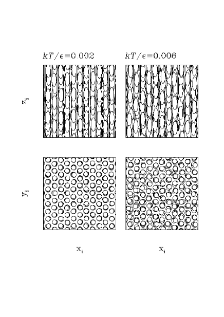
Figure 9: GCN model with $L/D=3$, some snapshots of the particle configuration taken at low temperature ($T^{*}=0.002$, BCC111(3) solid phase) and at intermediate temperature ($T^{*}=0.006$, columnar phase). The reduced pressure is $P^{*}=0.05$ in both cases. Above: side view, i.e., projection of particle coordinates onto the $x$-$z$ plane. Below: top view, i.e., projection of particle coordinates onto the $x$-$y$ plane. For clarity, in spite of their mutual interaction being soft, the particles are given sharp ellipsoidal boundaries, corresponding to a unitary short axis ($D$) and a long axis of $L=3D$. While the crystalline order along $z$ is lost already at $T^{*}=0.005$ (hence, it is there in the top-left panel while it is absent in the top-right panel), the triangular order within the $x$-$y$ plane is maintained up to the melting temperature (here, $T_{m}\simeq 0.0073$).

The only conclusion we can draw from the above chemical-potential study is that BCC111(3) is the most stable solid phase of the system (provided the pressure is not too low). However, a closer look at the DF profiles obtained from the simulation of BCC111(3) raises some doubts about the absolute stability of this phase at intermediate temperatures, whatever the pressure, calling for a different interpretation of the hitherto considered as BCC111(3) MC data. Take, for instance, the case of $P=0.05$. Upon increasing temperature, while $g_{\perp}$ keeps strongly peaked all the way to melting, the solid-like oscillations of $g_{\parallel}$ undergo progressive damping until they are washed out completely, suggesting a second-order (or very weak first-order at the most) transformation of BCC111(3) into a columnar phase before melting. This is illustrated in Figs. 6 and 7, where the DFs are plotted for a number of temperatures. A similar indication is got from the behavior of the smectic OP, see Fig. 8, whose highest maximum eventually deflates at practically the same temperature, $T^{*}\approx 0.005$, at which the oscillations of $g_{\parallel}$ disappear. Note that no appearance of a columnar phase is seen during the simulation of either BCC110(3) or BCC001(3), nor in the simulation of FCC001(3) for $P^{*}=0.01$. A slice of the columnar phase is depicted in Fig. 9 (right panels). In this phase, columns of stacked particles are arranged side by side, tightly packed together so as to project a triangular solid on the $x$-$y$ plane. Neighboring columns are not commensurate with each other, as implied by a completely featureless $g_{\parallel}$.

The probable reason for the instability of the smectic phase in the GCN model is the absence of an ad hoc mechanism for lateral attraction between the molecules, which is present instead in the model of Ref. deMiguel . By the way, hard ellipsoids do not show a smectic phase either Frenkel2 , at variance with (long) hard spherocylinders where particle geometry alone proves sufficient to stabilize a periodic modulation of the number density along $\hat{\bf z}$ Bolhuis .

Given the compelling evidence of a columnar phase in the GCN model, one may now ask whether the conclusions drawn from the chemical-potential data are all flawed. In particular, the $\mu$ curves that are tagged as BCC111(3) in Figs. 3 to 5 would be meaningless beyond a certain temperature $T_{c}<T_{m}$. In fact they are not, i.e., they retain full validity up to melting since the (nearly) continuous character of the transition from BCC111(3) to columnar allows one to safely continuate thermodynamic integration across the boundary, with the proviso that what previously treated as the BCC111(3) chemical potential beyond $T_{c}$ is to be assigned instead to the columnar phase.

As pressure goes up, the transition from BCC111(3) to columnar takes place at lower and lower temperatures. In order to exclude that the columnar phase too, likewise the fluid, will show reentrant behavior at low pressure, we have simulated the disordering of a BCC111(3) solid also for $P^{*}=0.02$ and 0.03 (in fact, no reentrance of the columnar phase is observed). Further points on the melting line for $P=0.01,0.02$, and 0.03 are fixed through the behavior of $g_{\perp}$ as a function of temperature. All in all, the overall GCN phase diagram appears as sketched in Fig. 10. This is similar to the phase portrait of the Gaussian-core model, see Fig. 1 of Ref. Prestipino2 , with the obvious exception of the columnar phase. There is a small discrepancy between the melting points as located through free-energy calculations (full dots in Fig. 10) and those assessed from the evolution of $g_{\perp}$ (open dots). In our opinion, this would mostly be attributed to the statistical error associated with the $\mu_{\rm ex}$ of the fluid in its reference state. Notwithstanding their limited precision, however, free-energy calculations are all but useless in identifying the structure of the solid phase. In conclusion, although some aspects of the equilibrium behavior of the GCN model remain still uncertain, especially with regard to the exact location of the solid-solid transition at low pressure, we are confident that the main features of the GCN phase diagram are correctly accounted for by Fig. 10.

Summing up, there are at least two conceivable and mutually exclusive paths for the thermal disordering of a liquid-crystal solid (aside from a direct transformation of it into a nematic phase). One is through the formation of a smectic phase, which eventually transforms into a nematic fluid. A second possibility is a more gradual release of crystalline order by the appearance of a columnar phase as intermediate stage between the solid and the nematic phase. Our study showed that it is this second scenario that occurs in the GCN model, with no evidence whatsoever of a smectic phase.

V Conclusions

We have introduced a liquid-crystal model of softly-repulsive parallel ellipsoids, named the Gaussian-core nematic (GCN) model, aiming at a complete characterization of its phase behavior, including the solid sector. This requires a preliminary identification of all relevant solid structures, which is generally a far-from-trivial task to be accomplished for model liquid crystals Pfleiderer . Through a careful scrutiny of as many as eleven uniaxially-deformed cubic and hexagonal phases, we obtained a thorough description of the $T=0$ equilibrium phase portrait of the GCN model, identifying its ground state at any given pressure. In doing so, we discovered a rich and absolutely unexpected structural degeneracy, which is only lifted by going to $T>0$. At low temperature, and for not too low pressures, our free-energy calculations indicate that a GCN system with an aspect ratio of 3 is found in just one solid phase, i.e., a stretched BCC solid with the molecules oriented along [111]. Only near zero pressure, the stable phase becomes a stretched FCC solid. With increasing temperature, the BCC-type solid first undergoes a weak transition into a columnar phase, which still retains partial crystalline order, before melting completely into the nematic fluid.

It is worth emphasizing that our interest in the GCN model is purely theoretical, hard-core ellipsoids providing a more physically realistic model liquid crystal. One could even argue that a Gaussian repulsion is highly irrealistic for a liquid crystal. In real atomic systems, superposition of particle cores is strongly obstructed, whence the consideration of hard-core or steep inverse-power repulsion in the more popular models. However, unless the system density is very high, higher than considered in our study, repulsive Gaussian particles would effectively be blind to an inner hard core, which thus may or may not exist, as evidenced e.g. in the snapshots of Fig. 9 where particles appear well spaced out.

The GCN model is a “deformation” of Stillinger’s Gaussian-core model, well known for exhibiting a reentrant-melting transition. Various instances of reentrant behavior are also known for nematics Cladis and indeed one of the original motivations for the present work was searching for a new kind of reentrance, i.e., re-appearance of a more disordered phase with increasing pressure. With this study, we provide yet another example of reentrant behavior in a model nematic: While this is nothing but the analog of fluid-phase reentrance in the Gaussian-core model, the absolute novelty of our findings is in the nature of the intermediate phase, this being surprisingly columnar in a range of pressures rather than genuinely solid.

Table 1: GCN model for $L/D=3$: $T=0$ chemical potential $\mu(P)$ for eleven different solids and two values of $P^{*}$, 0.05 and 0.20. $N_{x},N_{y},N_{z}$ are the number of lattice points along the three spatial directions, $\rho=N_{x}N_{y}N_{z}/V$ is the density, and $\alpha$ is the stretching ratio (for the SH111 lattice, $\alpha$ is the so-called $c/a$ ratio). $N_{x},N_{y},N_{z}$ have been chosen so large that the rounding-off error on the total potential energy per particle, $U/N$, due to the finite lattice size is negligible. The numerical precision on $\rho$ and $\alpha$ is of one unit on the last decimal digit. Looking at the Table, the most stable structures at both pressures are five degenerate crystals, actually belonging to three distinct types which are exemplified by BCC001(3) (equivalent to FCC001(2.12) up to a dilation), BCC110(3), and BCC111(3) (equivalent to SC111(1.5)) – within brackets is the value of $\alpha$.

crystal	$N_{x},N_{y},N_{z}$	$\rho(0.05)$	$\alpha(0.05)$	$\mu(0.05)$	$\rho(0.20)$	$\alpha(0.20)$	$\mu(0.20)$
FCC001	10,20,10	0.086	2.12	0.855724	0.157	2.12	2.093695
BCC001	14,14,10	0.086	3.00	0.855724	0.157	3.00	2.093695
SC001	20,20,8	0.086	3.00	0.881586	0.158	3.00	2.105241
FCC110	16,12,12	0.086	3.00	0.856391	0.157	3.00	2.094368
BCC110	10,28,8	0.086	3.00	0.855724	0.157	3.00	2.093695
SC110	14,18,10	0.086	3.00	0.881586	0.158	3.00	2.105241
FCC111	16,18,9	0.086	3.00	0.856391	0.157	3.00	2.094368
BCC111	12,12,18	0.086	3.00	0.855724	0.157	3.00	2.093695
SC111	12,12,18	0.086	1.50	0.855724	0.157	1.50	2.093695
HCP111	18,20,10	0.086	3.00	0.856429	0.157	3.02	2.094474
SH111	18,20,9	0.086	2.75	0.870014	0.158	2.69	2.099565

Figure 1: $T=0$ equilibrium behavior of the GCN model with $L/D=3$. Left: $T=0$ chemical potential $\mu(P^{*})$ of various crystals relative to BCC110(3), which thus serves as the zero or reference level. The reduced pressure $P^{*}$ is incremented by steps of 0.01. Note that, for all $P$, the five crystals FCC001(2.12), BCC001(3), BCC110(3), BCC111(3), and SC111(1.5) are degenerate ($\Delta\mu=0$). Other data points are for FCC001 (continuous line; $\alpha=3$ for $P^{*}=0.01$, being $\alpha=2.12$ otherwise), FCC110(3) and FCC111(3) (dotted line), HCP111 (open dots), SH111 (open squares), SC001(3) and SC110(3) (dashed line). Right: Resulting equation of state in the pressure range from 0 to 0.30. FCC001(3) (open triangle) is stable at very low pressure, up to slightly less than 0.02, while FCC001(2.12), BCC001(3), etc. (open dots) prevail for higher pressures.

Figure 2: GCN model with $L/D=3$, chemical-potential results for $T^{*}=0.002$. In the picture, we plot the reduced chemical potential of the three $T=0$ degenerate structures that exist for not too low pressure, taking BCC111(3) for reference. The latter phase gives the most stable solid for any $P$ in the range from 0.05 to 0.20 (and, most likely, even further). The $\mu$ curves are obtained by thermodynamic integration of volume MC data, using as initial conditions those specified by the Frenkel-Ladd calculations that were carried out at $P^{*}=0.05$. Though the reported $\mu$ values for the BCC-type solids are very close to each other and also affected by some numerical noise, the higher stability of BCC111(3) cannot be truly called into question – a regular pattern is clearly seen behind each curve.

Figure 3: GCN model with $L/D=3$, chemical-potential results for $P^{*}=0.05$: Chemical potential of the fluid phase (dotted line) as compared with those of the competing solid phases for that pressure (BCC001(3), long-dashed line; BCC110(3), dashed line; BCC111(3), continuous line). While the BCC111(3) solid is stable at low temperature, the fluid phase overcomes it in stability for higher temperatures. This is more clearly seen in the inset, where chemical-potential differences are reported, taking the fluid $\mu$ for reference. The melting temperature for $P^{*}=0.05$, which is where the continuous line crosses zero, is estimated to be $T^{*}\simeq 0.0073$.

Figure 4: GCN model with $L/D=3$, chemical-potential results for $P^{*}=0.12$. Same notation as in Fig. 3, except for the absence of data for BCC001(3), which were not computed. Despite this, a look at the results in Figs. 2 and 3 give us confidence that the chemical potential of BCC001(3) will be closer to that of BCC110(3) than is for $P^{*}=0.05$.

Figure 5: GCN model with $L/D=3$, chemical-potential results for $P^{*}=0.20$. Same notation as in Figs. 3 and 4.

Figure 6: GCN model with $L/D=3$, distribution functions of BCC111(3) for $P^{*}=0.05$. Left: $T^{*}=0.002$. Right: $T^{*}=0.003$. The strenght of crystalline order along $\hat{\bf z}$, as measured by the amplitude of $g_{\parallel}$ oscillations, reduces with increasing temperature, until complete disorder is left above $T^{*}\simeq 0.005$ (see next Fig. 7). Considering that the crystallinity within the $x$-$y$ plane persists well beyond $T^{*}=0.005$ (the spatial modulation of $g_{\perp}$ remains solid-like beyond this temperature and up to melting), we conclude that the GCN system is found in a columnar phase for $0.005<T<T_{m}$.

Figure 7: GCN model with $L/D=3$, distribution functions of BCC111(3) for $P^{*}=0.05$. Left: $T^{*}=0.004$. Right: $T^{*}=0.005$.

Figure 8: GCN model with $L/D=3$, smectic order parameter $\tau(\lambda)$ of BCC111(3) for $P^{*}=0.05$. The behavior of $\tau(\lambda)$ faithfully reproduces that seen for $g_{\parallel}(z)$ (cf. Figs. 6 and 7): The deflating of the highest $\tau(\lambda)$ maximum with increasing temperature closely follows the thermal damping of $g_{\parallel}(z)$ oscillations.

Figure 10: GCN model with $L/D=3$, sketch of the phase diagram on the $T$-$P$ plane. The full dots mark the location of the melting transition as extracted from our free-energy calculations. Open symbols refer instead to the transition thresholds as given by a visual inspection of the DF profiles. Though the latter melting-point estimates are more easily obtained than the former, the free-energy study was essential to identify the correct solid structure of the GCN model at not too low pressure. To help the eye, tentative phase boundaries are drawn as continuous (i.e., first-order) and dashed (nearly second-order) lines through the transition points. In the low-pressure region, the solid-solid boundary is highly hypothetical since we have no data there.

References

- (1) D. Frenkel and A. J. C. Ladd, J. Chem. Phys. 81, 3188 (1984); see also J. M. Polson, E. Trizac, S. Pronk, and D. Frenkel, J. Chem. Phys. 112, 5339 (2000).
- (2) F. Saija and S. Prestipino, Phys. Rev. B 72, 024113 (2005).
- (3) S. Prestipino, F. Saija, and P. V. Giaquinta, Phys. Rev. E 71, 050102(R) (2005).
- (4) S. Prestipino, F. Saija, and P. V. Giaquinta, J. Chem. Phys. 123, 144110 (2005).
- (5) F. H. Stillinger, J. Chem. Phys., 65, 3968 (1976).
- (6) A. Lang, C. N. Likos, M. Watzlawek, and H. Löwen, J. Phys.: Condens. Matter, 12, 5087 (2000).
- (7) D. Frenkel, B. M. Mulder, and J. P. McTague, Phys. Rev. Lett. 52, 287 (1984).
- (8) A. Stroobants, H. N. W. Lekkerkerker, and D. Frenkel, Phys. Rev. A 36, 2929 (1987).
- (9) J. A. C. Veerman and D. Frenkel, Phys. Rev. A 41, 3237 (1990); ibidem, 43, 4334 (1991).
- (10) P. Bolhuis and D. Frenkel, J. Chem. Phys. 106, 666 (1997).
- (11) C. Vega, E. P. A. Paras, and P. A. Monson, J. Chem. Phys. 96, 9060 (1992); ibidem, 97, 8543 (1992).
- (12) P. Pasini and C. Zannoni eds., Advances in the Computer Simulations of Liquid Crystals (NATO-ASI Series, 1998).
- (13) S. Singh, Phys. Rep. 324, 107 (2000).
- (14) E. de Miguel and E. Martin del Rio, Phys. Rev. Lett. 95, 217802 (2005).
- (15) B. Widom, J. Chem. Phys. 39, 2808 (1963).
- (16) After completion of this paper, we became aware of the discovery, reported in P. Pfleiderer and T. Schilling, cond-mat/0612151, of a new stable crystal phase in freely-standing hard ellipsoids. This further demonstrates that the solid structure of liquid crystals is generally difficult to anticipate, even when the model system is the simplest as possible.
- (17) The first example of such behavior was discovered by P. E. Cladis, Phys. Rev. Lett. 35, 48 (1975); see also Ref. deMiguel and references therein.