Targeted Supervised Contrastive Learning for Long-Tailed Recognition

Abstract

Real-world data often exhibits long tail distributions with heavy class imbalance, where the majority classes can dominate the training process and alter the decision boundaries of the minority classes. Recently, researchers have investigated the potential of supervised contrastive learning for long-tailed recognition, and demonstrated that it provides a strong performance gain. In this paper, we show that while supervised contrastive learning can help improve performance, past baselines suffer from poor uniformity brought in by imbalanced data distribution. This poor uniformity manifests in samples from the minority class having poor separability in the feature space. To address this problem, we propose targeted supervised contrastive learning (TSC), which improves the uniformity of the feature distribution on the hypersphere. TSC first generates a set of targets uniformly distributed on a hypersphere. It then makes the features of different classes converge to these distinct and uniformly distributed targets during training. This forces all classes, including minority classes, to maintain a uniform distribution in the feature space, improves class boundaries, and provides better generalization even in the presence of long-tail data. Experiments on multiple datasets show that TSC achieves state-of-the-art performance on long-tailed recognition tasks. Code is available here.

1 Introduction

Real-world data often has a long tail distribution over classes: A few classes contain many instances (head classes), whereas most classes contain only a few instances (tail classes). For critical applications, such as medical diagnosis, autonomous driving, and fairness, the data are by their nature heavily imbalanced, and the minority classes are particularly important (minority classes can be patients or accidents [41, 49, 51]). Interest in such problems has motivated much recent research on imbalanced classification, where the training dataset is imbalanced or long-tailed but the test dataset is equally distributed among classes [24, 46, 50, 4, 49].

Long-tailed and imbalanced datasets pose major challenges for classification tasks leading to a significant performance drop [1, 2, 8, 52, 48]. Techniques such as data re-sampling [5, 40, 2, 1] and loss re-weighting [4, 9, 11, 25, 26, 3] can improve the performance of tail classes but typically harm head classes [24]. Recently, researchers have investigated the potential of supervised contrastive learning for long-tailed recognition, and demonstrated that it provides a strong performance gain [23]. They further proposed $k$-positive contrastive learning (KCL), a variant of supervised contrastive learning that yields even better performance on long-tailed datasets.

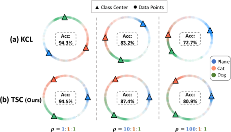
Figure 1: Test data feature distribution of (a) k-positive contrastive learning (KCL) and (b) TSC for three classes of CIFAR10 (plane, cat, dog), for different training data imbalance ratios $\rho$. With high imbalance ratio, class centers learned by KCL exhibit poor uniformity while class centers learned by TSC are still uniformly distributed and thus TSC achieves better performance (where Acc refers to Accuracy on test data).

However, while supervised contrastive learning can be beneficial, applying the contrastive loss (including the KCL loss) to imbalanced data can yield poor uniformity, which hampers performance. Uniformity is a desirable property [46]; it refers to that in an ideal scenario supervised contrastive learning should converge to an embedding where the different classes are uniformly distributed on a hypersphere [46, 19]. Uniformity maximizes the distance between classes in the feature space, i.e., maximizes the margin. As a result, it improves generalizability.

But, when the classes are imbalanced, training naturally puts more weight on the loss of majority classes and less weight on that of minority classes. As a result, the classes are no longer uniformly distributed in the feature space. To illustrate this issue, we consider three classes from CIFAR-10: dog, cat, and plane. We train a KCL model [23] on this data for different imbalance ratios, $\rho$. For visualization clarity we use a 2D feature space. As seen in Fig. 1(a), when the classes are balanced (i.e., $\rho$=1:1:1), the centers of the three classes are uniformly distributed in the KCL feature space. In contrast, when the imbalance ratio is high (e.g., $\rho$=100:1:1), the classes with fewer training instances start to collapse into each other, leading to unclear and inseparable decision boundaries, and thus lower performance. This is because the imbalanced data distribution naturally puts more weight on the uniformity loss between the head class and the tail classes, and less weight on that between the two tail classes, making the distance between head and tail classes much larger than the distance between two tail classes. The more imbalanced the long-tailed data, the more biased and less uniformly distributed the feature space.

One may attempt to fix this problem by oversampling the tail classes or re-weighting the loss function. However, as shown in [24], those methods overfit tail classes and improve tail-class performance at the expense of head classes, and thus harm the quality of the learned features. Therefore, a method that performs instance-balanced sampling while still being able to learn a uniform feature space is needed.

In this paper, we propose targeted supervised contrastive learning (TSC) for long-tailed recognition. To avoid the feature space being dominated and biased by head classes, we generate the optimal locations of class centers in advance (i.e., off-line). We call these uniformly distributed points class targets. We then devise an online matching-training scheme that performs contrastive training while adaptively matching samples from each class to one of the targets. As shown in Fig. 1(b), TSC learns a class-balanced feature space regardless of the imbalance ratio of the training set.

Note that one cannot simply match any target point with any class. Though the targets are uniformly distributed in the feature space, the distance between two targets can vary widely. For example, if the number of classes in Fig. 1 was 10 instead of 3, then though the targets are uniformly distributed, some targets will be closer to each other than the rest. Thus, our matching-training scheme has to ensure that classes that are semantically close (e.g., cat and dog) converge to nearby targets, and classes that are semantically farther apart converge to relatively distant targets.

We evaluate TSC on long-tailed benchmark datasets including CIFAR-10-LT, CIFAR-100-LT, ImageNet-LT, and iNaturalist, and show that it improves the state-of-the-art (SOTA) performances on all of them.

To summarize, this paper makes the following contributions:

• It introduces TSC, a novel framework for long-tailed recognition that avoids the feature space being dominated and biased by head classes.

• It empirically shows that supervised contrastive learning baselines can suffer from poor uniformity when applied to long-tailed recognition, which degrades their performances.

• It further shows that TSC achieves SOTA long-tailed recognition performances on benchmark datasets, demonstrating the effectiveness of the proposed method.

2 Related Works

Imbalanced Learning and Long-tailed Recognition. Real-world data typically follows a long-tailed or imbalanced distribution, which biases the learning towards head classes, and degrades performance on tail classes [49, 54]. Conventional methods have focused on designing class re-balancing paradigms through data re-sampling [5, 40, 2, 1] or adjusting the loss weights for different classes during training [4, 9, 11, 25, 26, 3]. However, such methods improve tail class performance at the expense of head class performance [24]. Researchers have also tried to improve long-tailed recognition by using ensembles over different data distributions[57, 46, 53], i.e., they re-organize long-tailed data into groups, train a model per group, and combine individual models in a multi-expert framework, or by using a distillation label generation module guided by self-supervision[33]. Ensemble-based and distillation-based methods have been shown to be orthogonal to methods operating on a single model and could leverage improvements in single-model methods to improve the performance.

Recent works [24, 57, 51] show that decoupling representation learning from classifier learning can lead to good features, which motivates the use of feature extractor pre-training for long-tailed recognition. The authors of [50] introduced a self-supervised pre-training initialization that alleviates the bias caused by imbalanced data. The authors of [23] further show that self-supervised learning can improve robustness to data imbalance, and introduce k-positive contrastive learning (KCL). Our work builds on this literature, and introduces a new approach to dealing with data imbalance using pre-computed uniformly-distributed targets that guide the training process to achieve better uniformity and improved class boundaries.

Contrastive Learning. Recent years have witnessed a steady progress on self-supervised representation learning [39, 10, 22, 38, 12, 13, 17, 33, 14, 32, 15, 55, 56]. Contrastive learning [21, 6, 7, 27, 16, 45, 30, 20] has been outstandingly successful on multiple tasks [31, 47, 37]. The core idea of contrastive learning is to align the positive sample pairs and repulse the negative sample pairs. Many works [45, 43, 30, 42, 19] have made efforts to understand and explain its properties, as well as its effects on downstream tasks. In particular, [45] proves that contrastive learning asymptotically optimizes both alignment (closeness) of features from positive pairs, and uniformity of the induced distribution of the (normalized) features on the hypersphere. Supervised contrastive learning (SupCon) [27] extends contrastive learning to the fully-supervised setting. It selects the positive samples from data belonging to the same class and aligns them in the embedding space, while simultaneously pushing away samples from different classes. By leveraging class labels with a contrastive loss, SupCon surpasses the performance of the traditional supervised cross-entropy loss on image classification. Most work on contrastive learning focuses on balanced data. Recently however, researchers have applied contrastive learning to imbalanced and long-tailed classification and demonstrated improved performance[23, 50].

3 Method

TSC is a training framework for improving the uniformity of the latent feature distribution. It aims to learn representations where the centers of each class are distributed uniformly on a hypersphere, and thus obtain clear decision boundaries between classes. TSC is especially effective on long-tailed recognition tasks, since for traditional methods based on supervised contrastive loss, classes with fewer training instances could easily collapse with other tail classes, resulting in poor classification performance.

Fig. 2 shows the overview of TSC. The targets where we want to position the class centers on the hypersphere are pre-computed prior to training and kept fixed thereafter. During training, the target positions are assigned to the classes online, and a targeted supervised contrastive loss is designed to encourage samples from each class to move to the assigned target position.

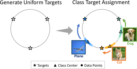
Figure 2: Illustration of TSC. It first computes the optimal targets for the class centers on the hypersphere. Then, during training, in each iteration, each target is assigned to the nearest class, and a targeted contrastive learning loss is designed to encourage the samples from each class to move to the assigned target position.

3.1 Target Generation

We first compute the optimal positions for the targets in the feature space. Since the test dataset is equally distributed among classes in long-tailed recognition, and the features in contrastive learning are positioned on a unit-hypersphere $\mathcal{S}^{d-1}=\{u\in\mathbb{R}^{d}:||u||=1\}$ [6, 21], the ideal class targets should be uniformly distributed on this hypersphere. Note that computing these ideal target positions does not require access to the data, and only requires knowing the number of classes and the dimension of the feature space. Thus, similar to the uniformity loss defined in [45], we design the target positions of $C$ classes, $\{t^{*}_{i}\}_{i=1}^{C}$, as the minimizer of

$$\mathcal{L}_{u}(\{t_{i}\}_{i=1}^{C})=\frac{1}{C}\sum\limits_{i=1}^{C}\log\sum\limits_{j=1}^{C}e^{t_{i}^{T}\cdot t_{j}/\tau}.$$ (1)

Intuitively, we want the target positions on the hypersphere to be as far away from each other as possible. The ideal locations would be perfectly uniformly distributed on the hypersphere, forming the vertices of a regular simplex (i.e. $\exists\delta\in\mathbb{R},t_{i}^{T}\cdot t_{j}=\delta,\forall i,j,i\neq j$ and $\sum\limits_{i}t_{i}=0$)[19]. However, when the dimension of the hypersphere is not large enough (e.g., $d<(C-1)$), computing the minimum of the above equation analytically becomes very hard [19]. Therefore, $\{t^{*}_{i}\}_{i=1}^{C}$ are calculated by gradient descent on $\mathcal{L}_{u}$, where $t_{i}$ is restricted to be on the hypersphere. Note that the minimum of $\mathcal{L}_{u}$ after gradient descent will be equal to its analytical minimum when $d\geq(C-1)$.

3.2 Matching-Training Scheme

Class-Target Assignment. Once we obtain a set of target positions, we need to assign a class label to each target. One way to do so is to randomly assign class labels to target positions. However, this will lead to a feature space with very poor semantics. This is because some target positions may be close to each other on the hypersphere and some are far away, especially when the number of classes is large (e.g., ImageNet and iNaturalist). Ideally, classes that are semantically close to each other should be assigned to target positions that are also close to each other.

It is hard however to accurately quantify semantic closeness between two classes. Even if we could quantify it, i.e., there is a well-defined “semantic distance” between two classes, it is computationally hard (i.e., no poly-time solution) to compute the optimal assignment that matches classes with target positions while keeping the semantic distance between classes consistent with the euclidean distance between their targets.

To solve this problem, we design a heuristic algorithm that finds a good assignment, while preserving the semantic structure of the feature space. Instead of pre-computing the assignment, we do it adaptively during training. Specifically, after each iteration in the training process, we use the Hungarian Algorithm [29] to find the assignment $\{\sigma^{*}_{i}\}_{i=1}^{C}$ that minimizes the distance between the target positions and the normalized class centers assigned to them, i.e.:

$$\{\sigma^{*}_{i}\}_{i}=\operatorname*{arg\,min}\limits_{\{\sigma_{i}\}_{i}}\frac{1}{C}\sum\limits_{i=1}^{C}||t_{\sigma_{i}}-c_{i}||,$$ (2)

where $c_{i}=\frac{\sum\limits_{v_{j}\in F_{i}}v_{j}}{||\sum\limits_{v_{j}\in F_{i}}v_{j}||_{2}}$ and $F_{i}$ is the set of features from class $i$. In practice, since a batch may contain only a subset of all classes, we keep track of the centers of each class using a weighted moving average. To be specific, in every iteration, we compute the new class centers $c_{i}^{\prime}$ for each class in the batch, and update the recorded $c_{i}$ by $c_{i}\leftarrow 0.9\cdot c_{i}+0.1\cdot c_{i}^{\prime}$. As shown in Sec. 5.2, this assignment algorithm demonstrates good performance on preserving the semantic structure of the feature space.

Targeted Supervised Contrastive Loss. To leverage the assigned targets, we design a targeted supervised contrastive loss $\mathcal{L}_{TSC}$. Given a batch of data samples $\{(x_{i},y_{i})\}_{i=1}^{N}$, where $y_{i}\in[C]$ is the class label of $x_{i}$. Define $v_{i}$ as the features of $x_{i}$ on the unit-hypersphere $\mathcal{S}^{d-1}$, $\tilde{v_{i}}$ as the features generated by augmenting $x_{i}$, $V_{i}=\{v_{n}\}_{n=1}^{N}\backslash\{v_{i}\}$ as the current batch of features excluding $v_{i}$ and $V_{i,k}^{+}\subseteq V_{i}$ the positive set of $v_{i}$ containing $k$ features uniformly drawn from $\{v_{j}\in V_{i}:y_{j}=y_{i}\}$. Let $\tilde{V_{i}}=\{\tilde{v_{i}}\}\cup V_{i}$ and $\tilde{V_{i,k}^{+}}=\{\tilde{v_{i}}\}\cup V_{i,k}^{+}$. $\mathcal{L}_{TSC}$ is then defined as:

$$\begin{aligned} \mathcal{L}_{TSC}=-\frac{1}{N}\sum_{i=1}^{N}\Big{(}&\frac{1}{k+1}\sum_{v_{j}^{+}\in\tilde{V^{+}_{i,k}}}\log\frac{e^{v_{i}^{T}\cdot v_{j}^{+}/\tau}}{\sum\limits_{v_{j}\in\tilde{V_{i}}\cup U}e^{v_{i}^{T}\cdot v_{j}/\tau}}\\ &+\lambda\log\frac{e^{v_{i}^{T}\cdot c^{*}_{i}/\tau}}{\sum\limits_{v_{j}\in\tilde{V_{i}}\cup U}e^{v_{i}^{T}\cdot v_{j}/\tau}}\Big{)},\end{aligned}$$ (3)

where $U=\{t^{*}_{i}\}_{i=1}^{C}$ is the set of pre-compute targets, and $c^{*}_{i}=t^{*}_{\sigma^{*}_{y_{i}}}$ is the assigned target of the corresponding class. Note that the loss is the sum of two components. The first is a standard contrastive loss as used by KCL [23], whereas the second is a contrastive loss between the target and the samples in the batch. This latter loss moves the samples closer to the target of their class and away from the targets of other classes.

$\mathcal{L}_{TSC}$ forces projections from each class to be aligned with its assigned target, while distributing the targets uniformly on the hypersphere, and thus is beneficial for long-tailed recognition tasks.

4 Experiments

We evaluate TSC on multiple long-tailed benchmark datasets and demonstrate its superior performances.

4.1 Experiment Setup

We perform extensive experiments on benchmark datasets, like CIFAR-10-LT and CIFAR100-LT (The MIT License), and large-scale long-tailed datasets, such as ImageNet-LT (CC BY 2.0 license) [35] and iNaturalist (CC0, CC BY or CC BY-NC license) [44]. CIFAR10-LT and CIFAR-100-LT are sampled with an exponential decay across classes. The imbalance ratio $\rho$ is defined as the number of samples in the most frequent class divided by that of the least frequent class. Similar to previous works, we evaluate TSC on imbalance ratios of 10, 50 and 100 and a ResNet-32 backbone [50]. For ImageNet-LT and iNaturalist, we evaluate TSC on a ResNet-50 backbone [23, 24, 46].

Following [24, 23], we implement TSC on long-tailed recognition datasets using a two-stage training strategy. In the first stage, we train the representation encoder with the TSC loss. In the second stage, we train a linear classifier on top of the learned representation. For CIFAR-10-LT and CIFAR-100-LT, the linear classifier is trained with LDAM loss and class re-weighting. For ImageNet-LT and iNaturalist, the linear classifier is trained with CE loss and class-balanced sampling. We also empirically find that in the early training, it is better to first warm up the network by not assigning targets and training the network with just the KCL loss. Therefore, for ImageNet-LT and iNaturalist, we start the class target assignment after half of the total epochs. Following the KCL loss, we use $k=6$ for the TSC loss. We use the same data augmentations as previous works, including the non-contrastive learning baselines. We provide a detailed description of the implementation of our method in the appendix. All results are averaged over 3 trials with different random seeds.

There are mainly two types of works on long-tailed recognition: 1) single model training scheme design, such as new sampling strategies [24] or new losses [9, 4, 23], and 2) ensembling over different data distributions, which re-organizes long-tailed data into groups, trains a model per group, and combines individual models in a multi-expert framework. Prior work [46] shows that these two approaches are orthogonal and can be combined together to improve performance. Our work falls in the first type of works. Therefore, we first compare TSC with established state-of-the-art single model baselines, including [4, 24, 23, 28], and then show that the combination of TSC and ensemble-based models can further improve its performance. Also, the literature compares different baselines for different datasets [50, 23, 46]. Thus, for each dataset, we compare with the typical and SOTA baselines for that dataset.

4.2 Results

CIFAR-10-LT & CIFAR-100-LT. Table 1 compares TSC with state-of-the-art baselines on CIFAR-10-LT and CIFAR-100-LT. It shows that, unlike other SOTA methods, TSC demonstrates consistent improvements over all baselines on all imbalance ratios in both datasets. This demonstrates that TSC can be generalized to different imbalance ratios and datasets easily as its design does not require prior knowledge of the imbalance ratio of the dataset.

Table 1: Top-1 accuracy (%) of ResNet-32 on long-tailed CIFAR-10 and CIFAR-100. TSC consistently improves on past imbalanced learning techniques and achieves the best performance. Previous SOTA results for each imbalance ratio are colored with gray. We report the accuracy of our re-implemented KCL ($\dagger$) since they do not report their performance on CIFAR in [23].

Dataset	CIFAR-10-LT			CIFAR-100-LT
Imbalance Ratio ($\rho$)	100	50	10	100	50	10
CE	70.4	74.8	86.4	38.3	43.9	55.7
CB-CE [9]	72.4	78.1	86.8	38.6	44.6	57.1
Focal [34]	70.4	76.7	86.7	38.4	44.3	55.8
CB-Focal [9]	74.6	79.3	87.1	39.6	45.2	58.0
CE-DRW [4]	75.1	78.9	86.4	40.5	44.7	56.2
CE-DRS [4]	74.5	78.6	86.3	40.4	44.5	56.1
LDAM [4]	73.4	76.8	87.0	39.6	45.0	56.9
LDAM-DRW [4]	77.0	80.9	88.2	42.0	46.2	58.7
M2m-ERM [28]	78.3	-	87.9	42.9	-	58.2
M2m-LDAM [28]	79.1	-	87.5	43.5	-	57.6
KCL$\dagger$ [23]	77.6	81.7	88.0	42.8	46.3	57.6
TSC	79.7	82.9	88.7	43.8	47.4	59.0

ImageNet-LT. Table 2 compares TSC with state-of-the-art baselines on ImageNet-LT dataset. As shown in the table, TSC demonstrates significant improvements over the baselines based on cross-entropy loss. It outperforms $\tau$-norm by 5.7%, cRT by 5.1%, and LWS by 4.7%. It also improves over KCL [23] for all class splits (1.1% for many, 0.7% for medium and 0.9% for few). Note that TSC improves both the accuracy of the many split and that of the few split. This is because TSC not only improves the uniformity of the minority classes, but also improves the overall uniformity of the whole feature space, as is detailed in Sec. 5.1. This further demonstrates the effectiveness of the proposed TSC loss in improving uniformity across class centers and delivering clean boundaries between classes.

Table 2: TSC outperforms previous state-of-the-art single-model methods on ImageNet-LT. Previous SOTA results of each class split (many, medium, few, all) are colored with gray. Please note that the KCL accuracy for each class split reported in [23] does not match the reported accuracy on all classes (61.8*0.385+49.4*0.479+30.9*0.136=51.658 which cannot be rounded to 51.5), indicating that their reported results may have a typo. Therefore, we also report the result of our re-implemented KCL (denoted with $\dagger$), which achieves similar accuracy on all classes but slightly different accuracy on each split.

Methods	Many	Medium	Few	All
OLTR [35]	35.8	32.3	21.5	32.2
$\tau$-norm [24]	56.6	44.2	27.4	46.7
cRT [24]	58.8	44.0	26.1	47.3
LWS [24]	57.1	45.2	29.3	47.7
FCL [23]	61.4	47.0	28.2	49.8
KCL [23]	61.8	49.4	30.9	51.5
KCL $\dagger$	62.4	49.0	29.5	51.5
TSC	63.5	49.7	30.4	52.4

iNaturalist. Table 3 compares TSC with state-of-the-art baselines on iNaturalist dataset. TSC achieves the best performance among all baselines on all class splits, demonstrating its effectiveness in solving real-world long-tailed recognition problems such as natural species classification.

Table 3: TSC outperforms previous state-of-the-art single-model methods on challenging iNaturalist 2018 [44] dataset, which contains 8142 classes. Previous SOTA results for each class split (many, medium, few, all) are colored with gray.

Methods	Many	Medium	Few	All
CE	72.2	63.0	57.2	61.7
CB-Focal	-	-	-	61.1
OLTR [35]	59.0	64.1	64.9	63.9
LDAM + DRW [4]	-	-	-	64.6
cRT [24]	69.0	66.0	63.2	65.2
${\tau}$-norm [24]	65.6	65.3	65.9	65.6
LWS [24]	65.0	66.3	65.5	65.9
KCL [23]	-	-	-	68.6
TSC	72.6	70.6	67.8	69.7

Table 4: Top-1 accuracy on ImageNet-LT with ResNet-50. Combination of TSC and state-of-the-art ensemble-based method RIDE [46] can further improve its performance.

Methods	Many	Medium	Few	All
RIDE (2 experts) [46]	65.8	51.0	34.6	54.4
RIDE (3 experts) [46]	66.2	51.7	34.9	54.9
RIDE (4 experts) [46]	66.2	52.3	36.5	55.4
TSC+RIDE (2 experts)	68.4	51.3	36.4	55.9
TSC+RIDE (3 experts)	69.1	51.7	36.7	56.3
TSC+RIDE (4 experts)	69.2	52.4	37.9	56.9

Combination of TSC and ensembling method: In previous results, we compare TSC with established state-of-the-art single model baselines. Here we show that TSC can also be combined with a state-of-the-art ensemble-based method, RIDE [46], to further boost its performance. To implement TSC with RIDE, we simply replace the original stage-1 training in RIDE with TSC and keep the stage-2 routing training unchanged. As shown in Table 4, the combination of TSC and RIDE observes consistent improvements across all different number of experts. This further demonstrate the effectiveness of TSC on long-tailed recognition tasks.

5 Analysis

We conduct an extensive analysis of TSC to explain its advantages over the baselines. We also conduct thorough ablations to demonstrate the effectiveness of each component in the TSC pipeline.

5.1 Understanding the Learned Representations

In contrastive learning the features are regularized to fall on a hypershpere [6, 21], and the loss directly optimizes the distance between instances in the feature space. Thus, we can use distance in the feature space to evaluate the quality of learned representations. We propose several metrics to evaluate representations learned from long-tailed dataset, and study why TSC achieves better performance on long-tailed recognition than past work, e.g., KCL.

Intra-Class Alignment. One optimization goal of the contrastive loss is to minimize the distance between positive samples. Similar to [45], we define alignment under the supervised contrastive learning setting as the average distances between samples from the same class, where $F_{i}$ is the set of features from class $i$:

$$\textbf{A}=\frac{1}{C}\sum_{i=1}^{C}\frac{1}{|F_{i}|^{2}}\sum_{v_{j},v_{k}\in F_{i}}||v_{j}-v_{k}||_{2}.$$ (4)

Inter-Class Uniformity. Another optimization goal of contrastive loss is to maximize the distance between negative samples. Hence, we define inter-class uniformity under the supervised contrastive learning setting as the average distances between different class centers:

$$\textbf{U}=\frac{1}{C(C-1)}\sum_{i=1}^{C}\sum_{j=1,j\neq i}^{C}||c_{i}-c_{j}||_{2},$$ (5)

where $c_{i}$ is the center of samples from class $i$ on the hypersphere: $c_{i}=\frac{\sum\limits_{v_{j}\in F_{i}}v_{j}}{||\sum\limits_{v_{j}\in F_{i}}v_{j}||_{2}}$.

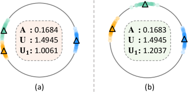
Figure 3: Example feature distributions of 3 classes with the same intra-class alignment and inter-class uniformity but different nearest neighborhood uniformity $U_{1}$. Because the nearest neighbor class is too close, the decision boundary between the green class and the orange class in (a) is not clean.

Neighborhood Uniformity. Though intra-class alignment and inter-class uniformity are important metrics to measure the quality of learned representations, they cannot evaluate how close one class is to its neighbors. For example, as shown in Fig. 3, although both (a) and (b) achieve the same alignment and uniformity, (b) shows better neighborhood uniformity in the feature space and clearer decision boundaries between the green class and the orange class.

Since what we really care about is only those classes that are too close to each other because the decision boundaries between them can be unclear, we define neighborhood uniformity as the distance to the top-$k$ closest class centers of each class:

$$\textbf{U}_{k}=\frac{1}{Ck}\sum_{i=1}^{C}\min_{j_{1},\cdots,j_{k}}(\sum_{l=1}^{k}||c_{i}-c_{j_{l}}||_{2}),$$ (6)

where $j_{1},\cdots,j_{k}\neq i$ are different classes.

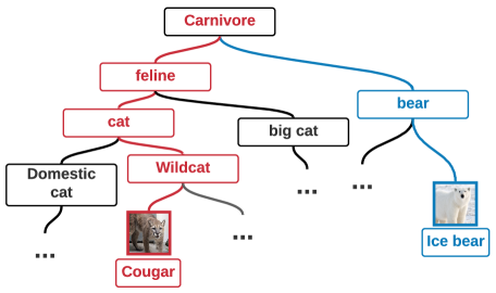
Figure 4: Illustration of semantic distance between two classes.

Reasonability. For better generalization, the learned feature space should also keep a reasonable semantic structure, i.e. ,classes that are semantically close to each other should also be close in feature space. Therefore, we define reasonability as the semantic distance between each class and its top-$k$ closest classes. The semantic distance of two classes is computed using WordNet hierarchy [36], which is a hierarchical structure that contains all ImageNet classes as leaf nodes. The semantic distance of two classes is then defined as the shortest distance between the two leaf nodes in WordNet hierarchy. For example, as shown in Fig. 4, the semantic distance between Cougar and Ice bear is 6.

Table 5: TSC achieves better uniformity, neighborhood uniformity and reasonability than KCL on ImageNet-LT, while keeping almost the same alignment. The $k$ for neighborhood uniformity and reasonability is set to 10. $\uparrow$ indicates larger is better, whereas $\downarrow$ indicates smaller is better.

Metric	Methods	Many	Medium	Few	All
A↓	KCL$\dagger$	0.71	0.69	0.72	0.70
	TSC	0.71	0.70	0.74	0.71
U↑	KCL$\dagger$	1.33	1.32	1.30	1.32
	TSC	1.38	1.38	1.37	1.38
U${}_{10}^{\uparrow}$	KCL$\dagger$	0.94	0.89	0.87	0.91
	TSC	1.02	1.02	1.05	1.02
R↓	KCL$\dagger$	7.35	7.25	7.42	7.31
	TSC	7.22	7.13	6.94	7.14
Acc.↑	KCL$\dagger$	62.4	49.0	29.5	51.5
	TSC	63.5	49.7	30.4	52.4

KCL vs. TSC. In Table 5, we compare the alignment, uniformity, neighborhood uniformity and reasonability of KCL and TSC on ImageNet-LT. The results highlight several good properties of TSC over KCL: 1.) TSC achieves better uniformity, neighborhood uniformity, and reasonability than KCL on all class splits, while keeping almost the same alignment as KCL. 2.) Although TSC’s uniformity is only 0.06 higher than that of KCL, its neighborhood uniformity (the average uniformity of the closest 10 classes) is 0.17 higher than that of KCL. Moreover, KCL’s neighborhood uniformity is even worse on tail classes, while TSC keeps consistent neighborhood uniformity over all classes. This demonstrates the effectiveness of TSC on keeping all classes away from each other, and thus allowing clearer decision boundaries between classes. 3.) TSC achieves better reasonability than KCL, especially on tail classes, showing that the learned feature space is not only uniform but also semantically reasonable.

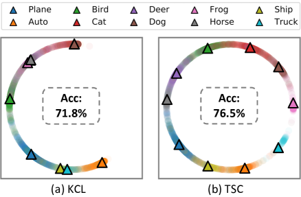
Figure 5: Feature distribution and accuracy of (a) KCL and (b) TSC on CIFAR-10-LT with imbalance ratio 100. In (a), the class centers of cat and dog collapse together, as well as the class centers of horse, deer, and frog.

Visualization. We can obtain more insights by visualizing the features learned by TSC and KCL. In Fig. 5, we visualize the features learned using KCL and TSC on CIFAR-10-LT with imbalance ratio of 100 and $d=2$. The triangles indicate the class centers. As shown in Fig. 5(a), features learned by KCL suffer from poor uniformity. Several class pairs collapse into each other, leading to unclear boundaries. We also see that when uniformity is quite poor, a large part of the feature space is left empty. On the other hand, Fig. 5(b) shows that features learned using TSC achieve good uniformity and clear separation between classes, hence achieve better classification performance.

5.2 Ablations

Table 6: Comparison between KCL, KCL with class-balanced sampling and TSC on CIFAR-10-LT and CIFAR-100-LT.

Dataset	CIFAR-10-LT			CIFAR-100-LT
Imbalance Ratio ($\rho$)	100	50	10	100	50	10
KCL$\dagger$	77.6	81.7	88.0	42.8	46.3	57.6
CB-KCL	75.5	80.2	87.1	41.5	45.5	56.8
TSC	79.7	82.9	88.7	43.8	47.4	59.0

Class-Balanced Sampling. Since KCL exhibits poor uniformity, one may think of improving its uniformity using class-balanced sampling. Table 6 compares KCL with class-balanced sampling with TSC. As shown in the table, class-balanced sampling gets even worse performance than standard KCL on both CIFAR-10 and CIFAR-100. This phenomenon is also shown in [24], where the author shows that instance-balanced sampling achieves the best results among different sampling strategies during representation learning. TSC uses instance-balanced sampling, and achieves good uniformity using pre-computed targets.

Table 7: Balanced positive sampling strategy improves less on TSC than on FCL on ImageNet-LT.

Methods	Many	Medium	Few	All
FCL [23]	61.4	47.0	28.2	49.8
KCL [23]	61.8	49.4	30.9	51.5
TSC (FCL)	62.7	49.2	30.1	51.8
TSC (KCL)	63.5	49.7	30.4	52.4

Benefits of Balanced Positive Samples. [23] has shown that sampling positive pairs in a balanced way (as done in KCL) is better than taking all samples of the same class as positives (as done in FCL). Therefore, TSC also builds on top of the KCL loss which samples the same number of positive pairs for each data point. However, we also notice that this balanced positive sampling strategy brings much less improvement to TSC than KCL. As shown in Table 7, the balanced positive sampling strategy in KCL improves 1.7% over FCL, while improves 0.7% over TSC with FCL. This is possibly because with a balanced feature space, the alignment within each class is also naturally balanced and therefore does not need the balanced positive sampling strategy, which further demonstrates the importance of a balanced feature space.

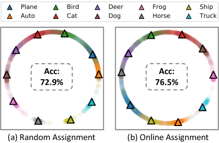
Figure 6: Comparison of feature distribution and accuracy using (a) random class assignment and (b) online assignment in TSC  on CIFAR-10-LT with imbalance ratio 100.

Table 8: TSC with and without online matching algorithm on ImageNet-LT.

Methods	Many	Medium	Few	All	R↓
KCL $\dagger$	62.4	49.0	29.5	51.5	7.31
TSC (random assign)	61.8	48.1	29.2	50.8	7.81
TSC (online matching)	63.5	49.7	30.4	52.4	7.14

Online Matching Algorithm. In Fig. 6(a), we show the performance of TSC with randomly assigned targets on CIFAR-10-LT, where the target for each class is randomly assigned at the beginning of training and fixed for the entire training process. To better visualize the features, the feature dimension of the output is set to 2. As shown in the figure, both methods achieve good uniformity on training data. However, the semantics in Fig. 6(a) are not reasonable, as semantically close classes are not nearby in the feature space, e.g., deer and horse. Similar results are also shown in Table 8, where we compare the reasonability of TSC with and without the online matching algorithm. Without the online matching algorithm, the reasonability of TSC is significantly worse than with it, resulting in much poorer generalization performance.

Table 9: $\mathcal{L}_{u}$ achieved with different random seeds during optimal targets generation for different numbers of classes.

# Class	10	100	1000	8142
seed = 0	14.286	14.286	14.287	14.297
seed = 1	14.286	14.286	14.287	14.297
seed = 2	14.286	14.286	14.287	14.297
seed = 3	14.286	14.286	14.287	14.297
seed = 4	14.286	14.286	14.287	14.297
std	3.2e-6	6.1e-6	1.8e-6	3.0e-6

Stability of Target Generation. An important step of our pipeline is to generate optimal targets. Since we use numerical approximation (SGD) to generate optimal targets, it is possible that the generated targets can achieve different minimum of $\mathcal{L}_{u}$ with different random seeds. Here we show the stability of our targets generation process. Table 9 shows the final $\mathcal{L}_{u}$ achieved by SGD with different random seeds. As shown in the table, with different random seed, the final $\mathcal{L}_{u}$ stays quite stable with negligible standard deviation. Therefore, the optimal targets generation process is stable.

6 Conclusion & Limitations

In this paper, we introduced targeted supervised contrastive learning (TSC) for long-tailed recognition. We empirically showed that, for unbalanced data, features learned by traditional supervised contrastive losses lead to reduced uniformity and unclear class boundaries, and hence poorer performance. By assigning uniformly distributed targets to each class during training, TSC avoids this problem, leading to a more uniform and balanced feature space. Extensive experiments on multiple datasets show that TSC achieves state-of-the-art single-model performance on all benchmark datasets for long-tailed recognition.

Nonetheless, TSC has some limitations. First, the optimal targets of TSC are computed using stochastic gradient descent. The analytical optimal solution of points on a hypersphere that minimize an energy potential remains an open problem (Thomson problem). Though TSC uses an approximate solution, the empirical results show consistent and significant performance gain. Second, TSC requires knowing the number of classes in advance to compute the targets; so, it is not applicable to problems where the number of classes is unknown. Despite these limitations, we believe that TSC provides an important step forward for long-tailed recognition, and delivers new insights on how data distribution affects key properties of contrastive learning.

References

- [1] Shin Ando and Chun Yuan Huang. Deep over-sampling framework for classifying imbalanced data. In Joint European Conference on Machine Learning and Knowledge Discovery in Databases, pages 770–785. Springer, 2017.
- [2] Mateusz Buda, Atsuto Maki, and Maciej A Mazurowski. A systematic study of the class imbalance problem in convolutional neural networks. Neural Networks, 106:249–259, 2018.
- [3] Jonathon Byrd and Zachary Lipton. What is the effect of importance weighting in deep learning? In International Conference on Machine Learning, pages 872–881. PMLR, 2019.
- [4] Kaidi Cao, Colin Wei, Adrien Gaidon, Nikos Arechiga, and Tengyu Ma. Learning imbalanced datasets with label-distribution-aware margin loss. Advances in Neural Information Processing Systems, 32:1567–1578, 2019.
- [5] Nitesh V Chawla, Kevin W Bowyer, Lawrence O Hall, and W Philip Kegelmeyer. Smote: synthetic minority over-sampling technique. Journal of artificial intelligence research, 16:321–357, 2002.
- [6] Ting Chen, Simon Kornblith, Mohammad Norouzi, and Geoffrey Hinton. A simple framework for contrastive learning of visual representations. In International conference on machine learning, pages 1597–1607. PMLR, 2020.
- [7] Xinlei Chen and Kaiming He. Exploring simple siamese representation learning. In Proceedings of the IEEE/CVF Conference on Computer Vision and Pattern Recognition, pages 15750–15758, 2021.
- [8] Ronan Collobert and Jason Weston. A unified architecture for natural language processing: Deep neural networks with multitask learning. In Proceedings of the 25th international conference on Machine learning, pages 160–167, 2008.
- [9] Yin Cui, Menglin Jia, Tsung-Yi Lin, Yang Song, and Serge Belongie. Class-balanced loss based on effective number of samples. In Proceedings of the IEEE/CVF conference on computer vision and pattern recognition, pages 9268–9277, 2019.
- [10] Carl Doersch, Abhinav Gupta, and Alexei A Efros. Unsupervised visual representation learning by context prediction. In Proceedings of the IEEE international conference on computer vision, pages 1422–1430, 2015.
- [11] Qi Dong, Shaogang Gong, and Xiatian Zhu. Imbalanced deep learning by minority class incremental rectification. IEEE transactions on pattern analysis and machine intelligence, 41(6):1367–1381, 2018.
- [12] Lijie Fan, Wenbing Huang, Chuang Gan, Stefano Ermon, Boqing Gong, and Junzhou Huang. End-to-end learning of motion representation for video understanding. In Proceedings of the IEEE Conference on Computer Vision and Pattern Recognition, pages 6016–6025, 2018.
- [13] Lijie Fan, Wenbing Huang, Chuang Gan, Junzhou Huang, and Boqing Gong. Controllable image-to-video translation: A case study on facial expression generation. In Proceedings of the AAAI Conference on Artificial Intelligence, volume 33, pages 3510–3517, 2019.
- [14] Lijie Fan, Tianhong Li, Rongyao Fang, Rumen Hristov, Yuan Yuan, and Dina Katabi. Learning longterm representations for person re-identification using radio signals. In Proceedings of the IEEE/CVF Conference on Computer Vision and Pattern Recognition, pages 10699–10709, 2020.
- [15] Lijie Fan, Tianhong Li, Yuan Yuan, and Dina Katabi. In-home daily-life captioning using radio signals. In European Conference on Computer Vision, pages 105–123. Springer, 2020.
- [16] Lijie Fan, Sijia Liu, Pin-Yu Chen, Gaoyuan Zhang, and Chuang Gan. When does contrastive learning preserve adversarial robustness from pretraining to finetuning? Advances in Neural Information Processing Systems, 34, 2021.
- [17] Lijie Fan, Shengjia Zhao, and Stefano Ermon. Adversarial localization network. In Learning with limited labeled data: weak supervision and beyond, NIPS Workshop, 2017.
- [18] Scott Fortin. The graph isomorphism problem. 1996.
- [19] Florian Graf, Christoph Hofer, Marc Niethammer, and Roland Kwitt. Dissecting supervised constrastive learning. In International Conference on Machine Learning, pages 3821–3830. PMLR, 2021.
- [20] Jean-Bastien Grill, Florian Strub, Florent Altché, Corentin Tallec, Pierre H Richemond, Elena Buchatskaya, Carl Doersch, Bernardo Avila Pires, Zhaohan Daniel Guo, Mohammad Gheshlaghi Azar, et al. Bootstrap your own latent: A new approach to self-supervised learning. 2020.
- [21] Kaiming He, Haoqi Fan, Yuxin Wu, Saining Xie, and Ross Girshick. Momentum contrast for unsupervised visual representation learning. In Proceedings of the IEEE/CVF Conference on Computer Vision and Pattern Recognition, pages 9729–9738, 2020.
- [22] Gao Huang, Danlu Chen, Tianhong Li, Felix Wu, Laurens Van Der Maaten, and Kilian Q Weinberger. Multi-scale dense convolutional networks for efficient prediction. arXiv preprint arXiv:1703.09844, 2, 2017.
- [23] Bingyi Kang, Yu Li, Sa Xie, Zehuan Yuan, and Jiashi Feng. Exploring balanced feature spaces for representation learning. In International Conference on Learning Representations, 2020.
- [24] Bingyi Kang, Saining Xie, Marcus Rohrbach, Zhicheng Yan, Albert Gordo, Jiashi Feng, and Yannis Kalantidis. Decoupling representation and classifier for long-tailed recognition. In International Conference on Learning Representations, 2019.
- [25] Salman Khan, Munawar Hayat, Syed Waqas Zamir, Jianbing Shen, and Ling Shao. Striking the right balance with uncertainty. In Proceedings of the IEEE/CVF Conference on Computer Vision and Pattern Recognition, pages 103–112, 2019.
- [26] Salman H Khan, Munawar Hayat, Mohammed Bennamoun, Ferdous A Sohel, and Roberto Togneri. Cost-sensitive learning of deep feature representations from imbalanced data. IEEE transactions on neural networks and learning systems, 29(8):3573–3587, 2017.
- [27] Prannay Khosla, Piotr Teterwak, Chen Wang, Aaron Sarna, Yonglong Tian, Phillip Isola, Aaron Maschinot, Ce Liu, and Dilip Krishnan. Supervised contrastive learning. Advances in Neural Information Processing Systems, 33, 2020.
- [28] Jaehyung Kim, Jongheon Jeong, and Jinwoo Shin. M2m: Imbalanced classification via major-to-minor translation. In Proceedings of the IEEE/CVF Conference on Computer Vision and Pattern Recognition, pages 13896–13905, 2020.
- [29] Harold W Kuhn. The hungarian method for the assignment problem. Naval research logistics quarterly, 2(1-2):83–97, 1955.
- [30] Tianhong Li, Lijie Fan, Yuan Yuan, Hao He, Yonglong Tian, Rogerio Feris, Piotr Indyk, and Dina Katabi. Making contrastive learning robust to shortcuts. arXiv preprint arXiv:2012.09962, 2020.
- [31] Tianhong Li, Lijie Fan, Yuan Yuan, and Dina Katabi. Unsupervised learning for human sensing using radio signals. In Winter Conference on Applications of Computer Vision, 2022.
- [32] Tianhong Li, Lijie Fan, Mingmin Zhao, Yingcheng Liu, and Dina Katabi. Making the invisible visible: Action recognition through walls and occlusions. In Proceedings of the IEEE/CVF International Conference on Computer Vision, pages 872–881, 2019.
- [33] Tianhao Li, Limin Wang, and Gangshan Wu. Self supervision to distillation for long-tailed visual recognition. In Proceedings of the IEEE/CVF International Conference on Computer Vision, pages 630–639, 2021.
- [34] Tsung-Yi Lin, Priya Goyal, Ross Girshick, Kaiming He, and Piotr Dollár. Focal loss for dense object detection. In Proceedings of the IEEE international conference on computer vision, pages 2980–2988, 2017.
- [35] Ziwei Liu, Zhongqi Miao, Xiaohang Zhan, Jiayun Wang, Boqing Gong, and Stella X Yu. Large-scale long-tailed recognition in an open world. In Proceedings of the IEEE/CVF Conference on Computer Vision and Pattern Recognition, pages 2537–2546, 2019.
- [36] George A Miller. Wordnet: a lexical database for english. Communications of the ACM, 38(11):39–41, 1995.
- [37] Pedro Morgado, Ishan Misra, and Nuno Vasconcelos. Robust audio-visual instance discrimination. In Proceedings of the IEEE/CVF Conference on Computer Vision and Pattern Recognition, pages 12934–12945, 2021.
- [38] Mehdi Noroozi and Paolo Favaro. Unsupervised learning of visual representations by solving jigsaw puzzles. In European conference on computer vision, pages 69–84. Springer, 2016.
- [39] Aaron van den Oord, Yazhe Li, and Oriol Vinyals. Representation learning with contrastive predictive coding. arXiv preprint arXiv:1807.03748, 2018.
- [40] Li Shen, Zhouchen Lin, and Qingming Huang. Relay backpropagation for effective learning of deep convolutional neural networks. In European conference on computer vision, pages 467–482. Springer, 2016.
- [41] Tony Shen, Ariel Lee, Carol Shen, and C Jimmy Lin. The long tail and rare disease research: the impact of next-generation sequencing for rare mendelian disorders. Genetics research, 97, 2015.
- [42] Yuandong Tian, Xinlei Chen, and Surya Ganguli. Understanding self-supervised learning dynamics without contrastive pairs. 2021.
- [43] Yonglong Tian, Chen Sun, Ben Poole, Dilip Krishnan, Cordelia Schmid, and Phillip Isola. What makes for good views for contrastive learning? 2020.
- [44] Grant Van Horn, Oisin Mac Aodha, Yang Song, Yin Cui, Chen Sun, Alex Shepard, Hartwig Adam, Pietro Perona, and Serge Belongie. The inaturalist species classification and detection dataset. In Proceedings of the IEEE conference on computer vision and pattern recognition, pages 8769–8778, 2018.
- [45] Tongzhou Wang and Phillip Isola. Understanding contrastive representation learning through alignment and uniformity on the hypersphere. In International Conference on Machine Learning, pages 9929–9939. PMLR, 2020.
- [46] Xudong Wang, Long Lian, Zhongqi Miao, Ziwei Liu, and Stella X Yu. Long-tailed recognition by routing diverse distribution-aware experts. arXiv preprint arXiv:2010.01809, 2020.
- [47] Haiping Wu and Xiaolong Wang. Contrastive learning of image representations with cross-video cycle-consistency. In Proceedings of the IEEE international conference on computer vision, 2021.
- [48] Tz-Ying Wu, Pedro Morgado, Pei Wang, Chih-Hui Ho, and Nuno Vasconcelos. Solving long-tailed recognition with deep realistic taxonomic classifier. In European Conference on Computer Vision, pages 171–189. Springer, 2020.
- [49] Yuzhe Yang, Hao Wang, and Dina Katabi. On multi-domain long-tailed recognition, generalization and beyond. arXiv preprint arXiv:2203.09513, 2022.
- [50] Yuzhe Yang and Zhi Xu. Rethinking the value of labels for improving class-imbalanced learning. In NeurIPS, 2020.
- [51] Yuzhe Yang, Kaiwen Zha, Ying-Cong Chen, Hao Wang, and Dina Katabi. Delving into deep imbalanced regression. In ICML, 2021.
- [52] Yuzhe Yang, Guo Zhang, Zhi Xu, and Dina Katabi. Me-net: Towards effective adversarial robustness with matrix estimation. In ICML, 2019.
- [53] Yifan Zhang, Bryan Hooi, Lanqing Hong, and Jiashi Feng. Test-agnostic long-tailed recognition by test-time aggregating diverse experts with self-supervision. arXiv preprint arXiv:2107.09249, 2021.
- [54] Yifan Zhang, Bingyi Kang, Bryan Hooi, Shuicheng Yan, and Jiashi Feng. Deep long-tailed learning: A survey. arXiv preprint arXiv:2110.04596, 2021.
- [55] Mingmin Zhao, Tianhong Li, Mohammad Abu Alsheikh, Yonglong Tian, Hang Zhao, Antonio Torralba, and Dina Katabi. Through-wall human pose estimation using radio signals. In Proceedings of the IEEE Conference on Computer Vision and Pattern Recognition, pages 7356–7365, 2018.
- [56] Mingmin Zhao, Yonglong Tian, Hang Zhao, Mohammad Abu Alsheikh, Tianhong Li, Rumen Hristov, Zachary Kabelac, Dina Katabi, and Antonio Torralba. Rf-based 3d skeletons. In Proceedings of the 2018 Conference of the ACM Special Interest Group on Data Communication, pages 267–281, 2018.
- [57] Boyan Zhou, Quan Cui, Xiu-Shen Wei, and Zhao-Min Chen. Bbn: Bilateral-branch network with cumulative learning for long-tailed visual recognition. In Proceedings of the IEEE/CVF Conference on Computer Vision and Pattern Recognition, pages 9719–9728, 2020.