Rethinking Graph Neural Networks for Anomaly Detection

Supplementary of “Rethinking Graph Neural Networks for Anomaly Detection”

Abstract

Graph Neural Networks (GNNs) are widely applied for graph anomaly detection. As one of the key components for GNN design is to select a tailored spectral filter, we take the first step towards analyzing anomalies via the lens of the graph spectrum. Our crucial observation is the existence of anomalies will lead to the ‘right-shift’ phenomenon, that is, the spectral energy distribution concentrates less on low frequencies and more on high frequencies. This fact motivates us to propose the Beta Wavelet Graph Neural Network (BWGNN). Indeed, BWGNN has spectral and spatial localized band-pass filters to better handle the ‘right-shift’ phenomenon in anomalies. We demonstrate the effectiveness of BWGNN on four large-scale anomaly detection datasets. Our code and data are released at https://github.com/squareRoot3/Rethinking-Anomaly-Detection.

1 Introduction

An anomaly or an outlier is a data object that deviates significantly from the majority of the objects, as if it was generated by a different mechanism (Han et al., 2011). As a well-established problem, anomaly detection has received much attention due to its vast applicable tasks, e.g., cyber security (Ten et al., 2011), fraud detection (Ngai et al., 2011), health monitoring (Bao et al., 2019), device failure detection (Sipple, 2020), to name a few. As graph data becomes ubiquitous in the Web era, graph information often plays a vital role in identifying fraudulent users or activities, e.g., friendship relations in a social network and transaction records on a financial platform. Consequently, as a crucial research direction, graph-based anomaly detection is necessary to be further explored (Noble & Cook, 2003; Ma et al., 2021).

Nowadays, Graph Neural Networks (GNNs) act as popular approaches for mining structural data, and are naturally applied for the graph anomaly detection task  (Bandyopadhyay et al., 2019; Kumar et al., 2018). Unfortunately, the vanilla GNNs are not well-suited for anomaly detection and suffer from the over-smoothing issue (Li et al., 2018; Wu et al., 2019). When GNN aggregates information from the node neighborhoods, it also averages the representations of anomalies and makes them less distinguishable. Thus, by intentionally connecting with large amounts of benign neighborhoods, the anomalous nodes may attenuate their suspiciousness, which results in the poor performance of the plain GNNs.

To remedy the issue, several GNN models have been proposed. We categorize the existing methods into three classes. That is, (1) applying attention mechanisms to correlate different neighbors through various views (Wang et al., 2019a; Cui et al., 2020; Liu et al., 2021a), (2) using the resampling strategy to aggregate neighborhood information selectively (Dou et al., 2020; Liu et al., 2020, 2021b), (3) designing auxiliary losses to enhance the network training power (Ding et al., 2019; Zhao et al., 2020, 2021). All these methods analyze the anomaly detection from the graph spatial domain. There are few works that address this problem from the spectral domain. Nevertheless, choosing a tailored spectral filter is a key component of GNN design, as the spectral filter determines the expressive power of GNN (Balcilar et al., 2020; He et al., 2021).

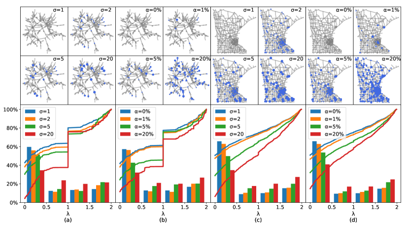
Figure 1: The effect of graph anomalies in the spatial domain (top) and spectral domain (bottom) with different anomaly degrees. The cases (a,c) are related to different standard deviation of anomalies (type (i), $\sigma=1,2,5,20$) while the cases (b,d) are about different fraction of anomalies (type (ii), $\alpha=0\%,1\%,5\%,20\%$).

To fill the above gap, we want to answer the question in this paper— how to choose a tailored spectral filter in GNN for anomaly detection? We take the first step towards analyzing anomalies via the lens of the graph spectrum (i.e., after the graph Fourier transform of node attributes). From Figure 1, we observe that low-frequency energy is gradually transferred to the high-frequency part, when the degree of anomaly becomes larger. We summarize this phenomenon as the ‘right-shift’ of spectral energy distribution, and further prove it on a Gaussian anomaly model in a rigorous manner. We validate the ‘right-shift’ phenomenon in a variety of graphs with synthetic or real-world anomalies. Through our analysis, we justify the necessity of spectral localized band-pass filters in graph anomaly detection.

Based on these findings, we propose Beta Wavelet Graph Neural Network (BWGNN) to better tackle the ‘right-shift’ phenomenon of graph anomalies. Although the frequency responses of existing works (Wu et al., 2021; He et al., 2021; Bo et al., 2021) can cover nearly all frequency profiles, these GNNs with adaptive filters cannot guarantee to be band-pass and spectral-localized (Balcilar et al., 2020). In fact, the design of frequency response in those works are not tailored to anomaly detection. Therefore, we invoke Hammond’s graph wavelet theory (Hammond et al., 2011) to develop our new graph neural network architecture. In contrast with the widely used Heat kernels (Donnat et al., 2018; Xu et al., 2019a; Li et al., 2021), the crux of our method is to propose the Beta kernel to address higher frequency anomalies via multiple flexible, spatial/spectral-localized, and band-pass filters.

To further facilitate this line of research, we release two large-scale real-world datasets as new graph anomaly detection benchmarks, including the T-Finance dataset based on a transaction network and the T-Social dataset based on a social network. Together with them, we conduct extensive experiments on four datasets in both supervised and semi-supervised settings. The proposed BWGNN shows superior performance over widely used graph neural networks and state-of-the-art graph anomaly detection methods.

2 Spectral Analysis of Graph Anomaly

To start with, we provide some necessary preliminaries of graph anomaly detection in Section 2.1. In Section 2.2, we give the theoretical insights of the ‘right-shift’ phenomenon and rigorously prove it on a Gaussian anomaly model. Towards that end, we validate our findings on graphs with synthetic anomalies in Section 2.3, and on real-world anomaly detection datasets in Section 2.4.

2.1 Preliminaries

Attributed Graph We define an attributed graph as $\mathcal{G}=\{\mathcal{V},\mathcal{E},\bm{X}\}$, where $\mathcal{V}=\{v_{1},v_{2},\cdots,v_{N}\}$ is the set of $N$ nodes, $\mathcal{E}=\{e_{ij}\}$ is the set of edges, and $e_{ij}=(v_{i},v_{j})$ represents an unweighted edge between nodes $v_{i}$ and $v_{j}$. Let $\bm{A}$ be the corresponding adjacency matrix, $\bm{D}$ be the degree matrix with $\bm{D}_{ii}=\sum_{j}\bm{A}_{ij}$. Each node $v_{i}$ has a $d$-dimensional feature vector $\bm{X}_{i}\in\mathbb{R}^{d}$, and the set of all node features is $\bm{X}=\{\bm{X}_{1},\bm{X}_{2},\cdots,\bm{X}_{N}\}$. In some applications, $\mathcal{G}$ is a multi-relational graph and multiple edge sets represent different relations between nodes.

Graph-based Anomaly Detection Let $\mathcal{V}_{a},\mathcal{V}_{n}$ be two disjoint subsets of $\mathcal{V}(i.e.,\mathcal{V}_{a}\cap\mathcal{V}_{n}=\varnothing)$, where $\mathcal{V}_{a}$ represents all the nodes labeled as anomalous and $\mathcal{V}_{n}$ represents all normal nodes. Graph-based anomaly detection is to classify unlabeled nodes in $\mathcal{G}$ into the normal or anomalous categories given the information of the graph structure $\mathcal{E}$, node features $\bm{X}$, and partial node labels $\{\mathcal{V}_{a},\mathcal{V}_{n}\}$. In this paper, we focus on node anomalies and assume that all edges in $\mathcal{G}$ are trusted, leaving structural anomalies for future work. Usually, there are far more normal nodes than anomalous nodes $(|\mathcal{V}_{a}|<<|\mathcal{V}_{n}|)$, thus graph-based anomaly detection can be regarded as an imbalanced binary node classification problem. The main difference is that anomaly detection focuses more on the unusual and deviated patterns in the dataset.

2.2 Theoretical Results

Problem Setup

Let the Laplacian matrix $\bm{L}$ be defined as $\bm{D}-\bm{A}$ (regular) or as $\bm{I}-\bm{D}^{-1/2}\bm{A}\bm{D}^{-1/2}$ (normalized), where $\bm{I}$ is an identity matrix. $\bm{L}$ is a symmetric matrix with eigenvalues, i.e., $0=\lambda_{1}\leq\cdots\leq\lambda_{N}$ and a corresponding orthonormal basis of eigenvectors $\bm{U}=(\bm{u}_{1},\bm{u}_{2},\cdots,\bm{u}_{N})$. Except for two endpoints $\lambda_{1}$ and $\lambda_{N}$, we can split other eigenvalues into the low frequencies $\{\lambda_{1},\lambda_{2},\cdots,\lambda_{k}\}$ and high frequencies $\{\lambda_{k+1},\lambda_{k+2},\cdots,\lambda_{N}\}$ with an arbitrary threshold $\lambda_{k}$.

Assume that $\bm{x}=(x_{1},x_{2},\cdots,x_{N})^{T}\in\mathbb{R}^{N}$ is a signal on $\mathcal{G}$, and $\bm{\hat{x}}=(\hat{x}_{1},\hat{x}_{2},\cdots,\hat{x}_{N})^{T}=\bm{U}^{T}\bm{x}$ is the graph Fourier transform of $\bm{x}$. We denote $\hat{x}_{k}^{2}/\Sigma_{i=1}^{N}\hat{x}_{i}^{2}$ as the spectral energy distribution at $\lambda_{k}(1\leq k\leq N)$. We summarize our theoretical and empirical findings as

The existence of anomalies leads to the ‘right-shift’ of spectral energy, which means the spectral energy distribution concentrates less in low frequencies and more in high frequencies.

To further justify the insight, we prove this interesting finding based on a probabilistic anomaly model (Han et al., 2011; Grubbs, 1969). The graph features are assumed to be identically independent drawn from a Gaussian distribution, i.e., $\bm{x}\sim\mathcal{N}(\mu e_{N},\sigma^{2}\bm{I}_{N})$, where $\mu e_{N}$ is an all-the-one vector. Here, the coefficient of variation $\sigma/|\mu|$ can be regarded as the degree of anomalies in $\bm{x}$, which is indeed a commonly used measure to describe the dispersion of a distribution (Kendall et al., 1946; Bedeian & Mossholder, 2000). When the fraction of anomalies in $\bm{x}$ increases, $\sigma/|\mu|$ becomes larger and indicates a more considerate degree of anomaly. Alternatively, if the distance between anomalies and the mean vector becomes larger, $\sigma/|\mu|$ also increases, representing a larger degree of anomalies.

To quantify how the spectral energy distribution changes with respect to the degree of anomalies in $\bm{x}$, we introduce a metric — energy ratio as below:

Definition 1 (Energy Ratio).

For any $1\leq k\leq N-1$, we define $k$-th low-frequency energy ratio as the accumulated energy distribution in the first $k$ eigenvalues:

$$\eta_{k}(\bm{x},\bm{L})=\frac{\sum_{i=1}^{k}\hat{x}_{i}^{2}}{\sum_{i=1}^{N}\hat{x}_{i}^{2}}.$$

A larger $\eta_{k}$ indicates that a larger part of the energy boils down to the first $k$ eigenvalues. In the following proposition, we shed light on how the degree of anomalies in $\bm{x}$ will affect $\eta_{k}$.

Proposition 2.

If $|\mu|\neq 0$ and $\bm{L}=\bm{D}-\bm{A}$, the expectation of the inverse of low-frequency energy ratio $\mathbb{E}_{\bm{x}}[1/\eta_{k}(\bm{x},\bm{L})]$ is monotonically increasing with the anomaly degree $\sigma/|\mu|$.

Proposition 2 indicates that an increased degree of anomaly enforces the spectral energy distribution to concentrate less on the low-frequency eigenvalues. The proof details can be found in Appendix A.

Unfortunately, the calculation of spectral energy ratio requires the eigen-decomposition of the graph Laplacian, which is time-consuming on large-scale graphs. To navigate such pitfalls, we introduce a more computational amenable metric to generally measure the effect of graph anomalies in the spectral domain.

Definition 3 (High-frequency Area).

Suppose that the low-frequency energy ratio curve $f(t)$ is defined as $f(t)=\eta_{k}(x,\bm{L})$ where $t\in[\lambda_{k},\lambda_{k+1})$ and $1\leq k\leq N-1$. The area between $f(t)$ and $g(t)=1$ is defined as the high-frequency area: $S_{\textnormal{high}}=\int_{0}^{\lambda_{N}}1-f(t)dt$.

Without the need of eigen-decomposition, $S_{\text{high}}$ can be computed by simple elementary manipulations:

$$S_{\text{high}}=\frac{\sum_{k=1}^{N}\lambda_{k}\hat{x}^{2}_{k}}{\sum_{k=1}^{N}\hat{x}_{k}^{2}}=\frac{\bm{x}^{T}\bm{L}\bm{x}}{\bm{x}^{T}\bm{x}}.$$ (1)

We refer the reader to Appendix B for further details. According to (1), spectral energy on low frequencies contributes less to $S_{\text{high}}$ after multiplying a small eigenvalue. For example, $S_{\text{high}}=0$ if the entire spectral energy concentrates on $\lambda_{1}=0$, and $S_{\text{high}}$ increases when spectral energy shifts to larger eigenvalues. Therefore, we can use the change of $S_{\text{high}}$ to describe the ‘right-shift’ phenomenon in the whole spectrum.

Furthermore, (1) reveals that the energy distribution of $\bm{x}$ in the spectral domain is closely related to the smoothness of $\bm{x}$ in the spatial domain — $\bm{x}^{T}\bm{L}\bm{x}$ will be smaller if signal $\bm{x}$ has closer values between connected nodes, which also reflects a smaller anomaly degree. In Appendix A, we additionally proof that $S_{\text{high}}$ is monotonically increasing with the anomaly degree $\sigma/|\mu|$, which matches the result in Proposition 2.

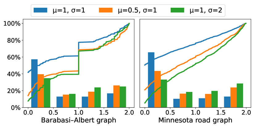
Figure 2: Spectral analysis of graph signal $\bm{x}\sim\mathcal{N}(\mu e_{N},\sigma^{2}\bm{I}_{N})$.

Table 1: Summary of dataset statistics and the comparison of anomaly effect on spectral energy distributions. The number in the parentheses is the lowest value of $\Delta S_{\text{high}}$ on each dataset.

	Statistics				Anomaly Effect ($\Delta S_{\text{high}}$)
Dataset	# Nodes	# Edges	Anomaly(%)	# Features	Drop-Anomaly	Drop-Random
Amazon	11,944	4,398,392	6.87%	25	-0.59% (-4.19%)	0.15% (-0.39%)
YelpChi	45,954	3,846,979	14.53%	32	-1.61% (-15.4%)	-0.04% (-1.14%)
T-Finance	39,357	21,222,543	4.58%	10	-0.34% (-0.92%)	0.09% (-0.01%)
T-Social	5,781,065	73,105,508	3.01%	10	-5.36% (-13.2%)	0.08% (-0.02%)

2.3 Validation on Synthetic Anomalies

To present our theoretical findings in a more intuitive way, we demonstrate it on different graphs with synthetic anomalies. In Figure 1, we study the effect of anomalies on two types of graph: a Barabási–Albert graph with 500 nodes on Figure 1 (a)-(b) and a Minnesota road graph with 2,642 nodes (Perraudin et al., 2014) in Figure 1 (c)-(d).

We first assume normal and anomalous nodes follow different distributions to better visualize the change of spectral energy under different anomaly degrees. For both graphs, the one-dimensional feature of each normal node is drawn from $\mathcal{N}(1,1)$, while the anomalous one is drawn from $\mathcal{N}(1,\sigma^{2})$ (i.e., $\sigma>1$). We analyze two variations of anomalies: (i) the fraction of anomalies is fixed to 5%, and the standard deviation of anomalies changes (i.e., $\sigma=1,2,5,20$); and (ii) the standard deviation of anomalies is fixed to 5 and the fraction of anomalies changes (i.e., $\alpha=0\%,1\%,5\%,20\%$). In the top half of Figure 1, we use blue circles to represent anomalous nodes in the spatial domain. Bigger blue nodes indicate a larger degree of anomaly. In the bottom half of Figure 1, we display the energy distribution of $\bm{x}$ in the spectral domain with various anomaly degrees. The colored histograms reflect the proportion of spectral energy in different eigenvalue intervals such as $[0,0.5)$, and the curves represent $f(t)$ in Definition 3.

We take the Barabási–Albert graph as an example. When the fraction of anomalies is 0%, most of the energy (60%) locates in the low frequency region $(\lambda<0.5)$. By contrast, when the anomaly degree becomes larger — increasing $\sigma$ and $\alpha$, the ratio of spectral energy for $\lambda>0.5$ becomes larger in the histogram. Also, the low-frequency energy ratio curve is almost monotonically decreasing on the interval $\lambda\in[0,2]$. The observation also holds for the Minnesota road graph.

Moreover, we further assume the features of all nodes are drawn from a single Gaussian distribution which strictly follows Proposition 2. We corroborate our theoretical findings on three cases: (1) the original features $\mu=1,\sigma=1$, (2) features with a smaller mean value $\mu=0.5,\sigma=1$, and (3) features with a larger variance $\mu=1,\sigma=2$. In Figure 2, both increasing the variance and decreasing the mean value lead to the ‘right-shift’ of spectral energy distributions, which is consistent with the result in Proposition 2.

2.4 Validation on Real-world Anomalies

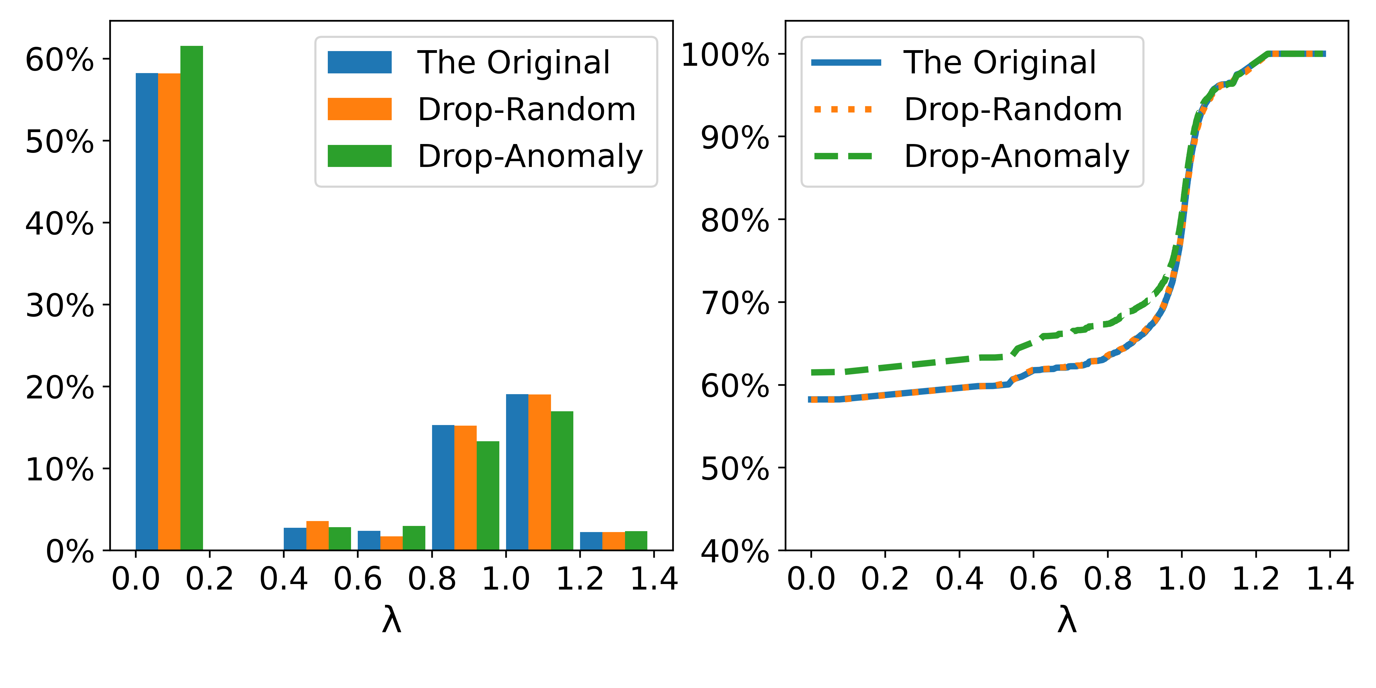
Figure 3: Comparison of the spectral energy distribution (left) and the energy ratio curve (right) between the original graph and two perturbed graphs in the Amazon dataset.

In real-world anomaly detection datasets, the node features may not strictly follow the Gaussian distribution. Nevertheless, we verify the generality of ‘right-shift’ on the real case. We introduce four industry datasets for different anomaly detection scenarios. We choose two widely used datasets in previous works (Liu et al., 2021b, 2020), including the Amazon dataset (McAuley & Leskovec, 2013) for user anomaly detection and the YelpChi dataset (Rayana & Akoglu, 2015) for review anomaly detection. We further construct two large-scale real-world datasets as new graph anomaly detection benchmarks, including the T-Finance dataset based on a transaction network and the T-Social dataset based on a social network. The statistics of these datasets are summarized in Table 1. More details about these datasets are in Section 4.1.

We first study the ‘right-shift’ phenomenon of anomalies in the Amazon dataset. We choose the last feature dimension and visualize the spectral energy in three views: (1) the origin graph, (2) the perturbed graph by dropping all anomalies, and (3) the perturbed graph by dropping the same number of random nodes. In Figure 3, compared with the origin graph, the spectral energy in the subgraph without anomalies concentrates more in low frequencies (i.e., $\lambda\in[0,0.2)$) and less in high frequencies (i.e., $\lambda\in[0.8,1.2)$). By contrast, dropping random nodes does not have the same effect. The ‘right-shift’ phenomenon in this case indicates that the frequency band around $\lambda=1$ has a strong connection with anomalies.

As the eigen-decomposition operation suffers from the heavy computational burden, especially on the other three large-scale datasets, we quantify the spectral effect by the high-frequency area introduced in Definition 3. We compare the original graph with two perturbed graphs. The relative change is calculated by $\Delta S_{\text{high}}=(\hat{S}_{\text{high}}-S_{\text{high}})/S_{\text{high}}$, in which $S_{\text{high}}$ and $\hat{S}_{\text{high}}$ denote the high-frequency area of the original graph and that of two perturbed graphs respectively.

We compute $\Delta S_{\text{high}}$ for each feature dimension and report the mean and lowest values in Table 1. Among all datasets, removing anomalies leads to the decrease of $S_{\text{high}}$, while dropping nodes randomly has limited effects on $S_{\text{high}}$. More specifically, on T-Social and Yelpchi, $S_{\text{high}}$ decreases more than 10% for the worst-case feature, which is impressive given that anomalies are few.

3 Methodology

The analysis in Section 2 shows that we need to focus on ‘right-shift’ effect when detecting graph anomalies. Unfortunately, most of the current GNNs are low-pass filters (Nt & Maehara, 2019; Wu et al., 2019) or adaptive filters (Defferrard et al., 2016; He et al., 2021; Dong et al., 2021; Levie et al., 2018) that are neither guaranteed to be band-pass nor spectral-localized (Balcilar et al., 2020). Since high-frequency anomalies account for only a small fraction and most spectral energy still concentrates on low frequencies, these adaptive GNNs may degrade to low-pass filters in this task.

To overcome this drawback, we propose our new graph neural network architecture based on Hammond’s graph wavelet theory (Hammond et al., 2011), which is band-pass in nature and can better address the ‘right-shift’ effect inheriting from anomalies. We first introduce the backgrounds of graph wavelet in Section 3.1. Then, we propose our graph Beta wavelet and demonstrate its good properties in Section 3.2. Based on Beta wavelets, we construct the Beta Wavelet Graph Neural Network (BWGNN) in Section 3.3. We discuss the differences between BWGNN and other related graph wavelets in Section 3.4.

3.1 Background: Hammond’s Graph Wavelet

The graph wavelet transform defined in (Hammond et al., 2011) starts with a ”mother” wavelet $\psi$ and employs a group of wavelets as bases, defined as $\mathcal{W}=(\mathcal{W}_{\psi_{1}},\mathcal{W}_{\psi_{2}},\cdots)$. Formally, applying $\mathcal{W}_{\psi_{i}}$ on a graph signal $x\in\mathbb{R}^{N}$ can be written as

$$\mathcal{W}_{\psi_{i}}(\bm{x})=\bm{U}g_{i}(\bm{\Lambda})\bm{U}^{T}\bm{x},$$ (2)

where $g_{i}(\cdot)$ is a kernel function in the spectral domain defined on $[0,\lambda_{N}]$, and $g_{i}(\bm{\Lambda})=\text{diag}(g_{i}(\lambda))$. Although Equation (2) is similar to the graph spectral convolution derived from Fourier transform, the kernel function $g_{i}$ in Hammond’s graph wavelet transform should satisfy the following additional requirements.

• According to the Parseval theorem, the wavelet transform needs to meet the admissibility condition:

  $$\small\int_{0}^{\infty}{\frac{|g_{i}(w)|^{2}}{w}}dw=C_{g}<\infty,$$

  which means $g_{i}$ should satisfy $g_{i}(0)=g_{i}(\infty)=0$ and perform like a band-pass filter in the spectral domain.

• The wavelet transform covers different frequency bands via band-pass filters of different scales $\{g_{1},g_{2},...\}$.

To avoid the eigen-decomposition of the graph Laplacian $\bm{L}$, the kernel function $g_{i}$ has to be a polynomial function, i.e., $\bm{U}g_{i}(\Lambda)\bm{U}^{T}=g_{i}(\bm{L})$ in most of the literature.

3.2 Beta Wavelet on Graph

Beta distribution often serves as a wavelet basis (De Oliveira & De Araújo, 2015) in computer vision applications (Amar et al., 2005; Jemai et al., 2010; ElAdel et al., 2016), but has not been utilized for mining graph data yet. Here we choose the Beta distribution as the graph kernel function and demonstrate that it meets the requirements of Hammond’s graph wavelet.

The probability density function of Beta distribution admits:

$$\beta_{p,q}(w)=\left\{\begin{array}[]{ll}\frac{1}{B(p+1,q+1)}w^{p}(1-w)^{q}&\text{if}\ \ w\in[0,1]\\ 0&\text{otherwise}\\ \end{array}\right.$$

where $p,q\in\mathbb{R}^{+}$ and $B(p+1,q+1)=p!q!/(p+q+1)!$ is a constant. As the eigenvalues of the normalized graph Laplacian $L$ satisfy $\lambda\in[0,2]$, we adopt $\beta_{p,q}^{*}(w)=\frac{1}{2}\beta_{p,q}(\frac{w}{2})$ to cover the complete spectral range of $L$. We further add the restrictions $p,q\in\mathbb{N}^{+}$ to ensure $\beta^{*}(p,q)$ is a polynomial, such that fast computation can be conducted. Thus, our Beta wavelet transform $\mathcal{W}_{p,q}$ can be written as:

$$\mathcal{W}_{p,q}=\bm{U}\beta^{*}_{p,q}(\bm{\Lambda})\bm{U}^{T}=\beta^{*}_{p,q}(\bm{L})=\frac{(\frac{\bm{L}}{2})^{p}(I-\frac{\bm{L}}{2})^{q}}{2B(p+1,q+1)}.$$

Let $p+q=C$ be a constant and our Beta wavelet transform $\mathcal{W}$ is constructed by a group of $C+1$ Beta wavelets with the same order:

$$\mathcal{W}=(\mathcal{W}_{0,C},\mathcal{W}_{1,C-1},\cdots,\mathcal{W}_{C,0}).$$ (3)

In this equation, $\mathcal{W}_{0,C}$ is a low-pass filter and others are band-pass filters of different scales. Besides, when $p>0$, the kernel function $\beta^{*}_{p,q}$ satisfies:

$$\int_{0}^{\infty}{\frac{|\beta^{*}_{p,q}(w)|^{2}}{w}}dw\leq\int_{0}^{2}\frac{dw}{2B(p+1,q+1)}<\infty.$$

Therefore, the proposed Beta wavelet transform $\mathcal{W}$ satisfies both two requirements of Hammond’s graph wavelet in Section 2.1.

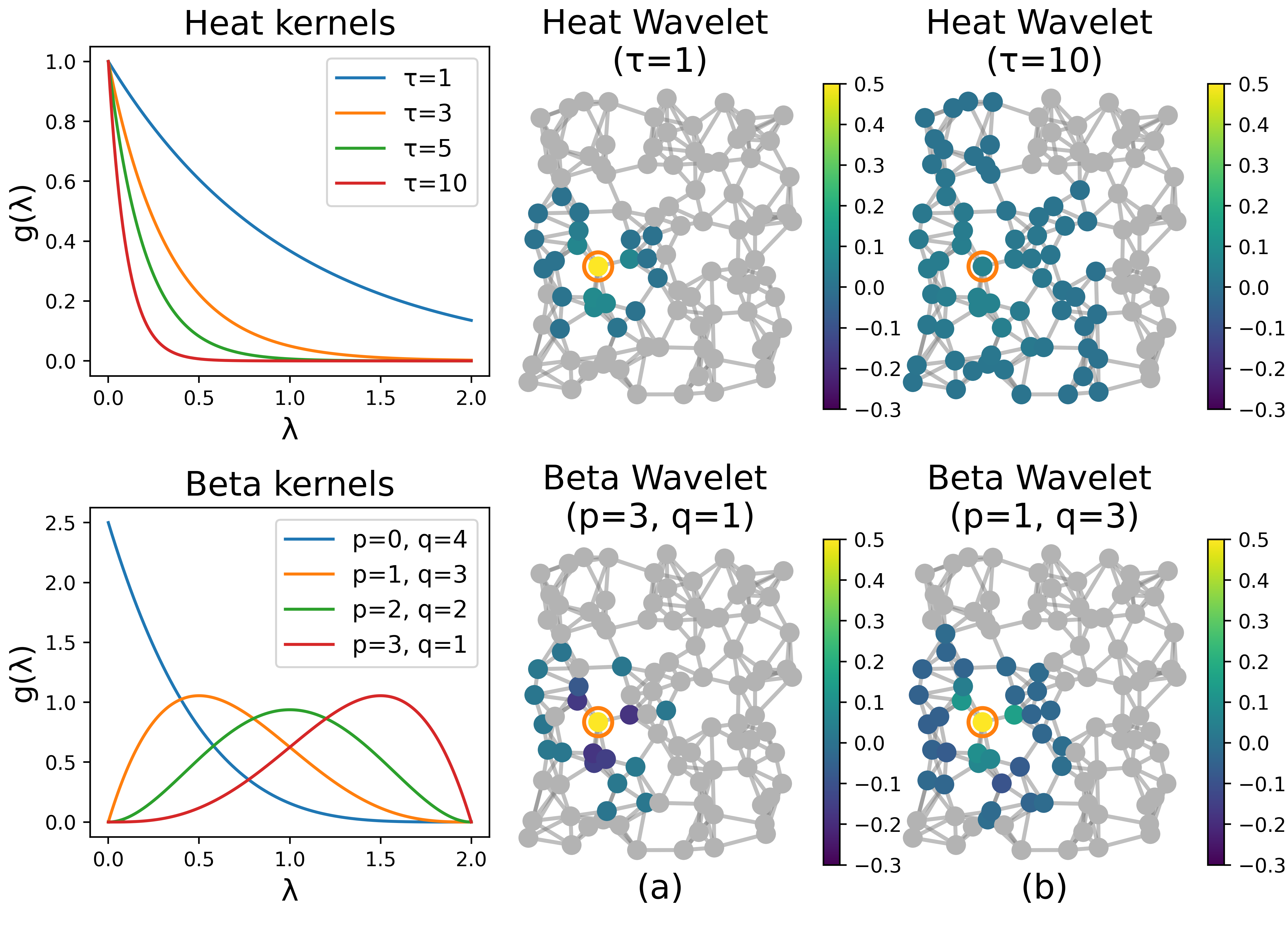
Figure 4: Comparison between Heat wavelets and Beta wavelets in the spectral domain (left) and the spatial domain (right).

Figure 4 compares a group of the proposed Beta wavelets ($C=4$) with the widely-used wavelet with Heat kernels (i.e., $g(\lambda)=e^{-\tau\lambda},\tau\in\{1,3,5,10\}$). The first column shows that Heat kernels are all low-pass filters in the spectral domain, while Beta kernels contain various filter types including low-pass and band-pass.

The right two columns in Figure 4 visualize the effect of graph wavelet transform on a randomly generated kNN graph. The responses with an absolute value less than 0.001 are marked as grey. For different scales, responses of heat wavelets are all positive, while those of Beta wavelets can be positive or negative in different channels. The diversified responses of the Beta graph wavelet transform show that it can capture not only the similarities but also the differences of nodes within a subgraph, thus a better neighborhood flexibility. This property can make the representations of anomalies more distinguishable.

The classic wavelet transform is well-known for its locality in time and frequency domains. As an analogy, we present two propositions about the good locality of Beta graph wavelets in spectral and spatial domains:

Proposition 4 (Spectral Locality).

Consider $p>0$, $q>0$ and $X\sim\beta^{*}_{p,q}$ where $\beta^{*}_{p,q}$ is band-pass, the mean and variance of $X$ are:

$$\mu= \mathbb{E}(X)=\frac{2(p+1)}{p+q+2}$$

$$\sigma= \textnormal{Var}(X)=\frac{4(p+1)(q+1)}{(p+q+2)^{2}(p+q+3)}.$$

When $p+q\rightarrow\infty$ satisfies $p=cq$, we have $\sigma\rightarrow 0$ and $\mu=\frac{2c}{c+1}$ can be any number between $(0,2)$.

Here, we use $p=cq$ to ensure $p$ and $q$ do not deviate dramatically. Proposition 4 can be directly derived from the properties of the Beta distribution. It shows $\beta^{*}_{p,q}$ can concentrate on any $\mu\in(0,2)$, which means Beta graph wavelets can be tailored to any specific frequency band for anomaly detection.

Proposition 5 (Spatial Locality).

Let $v_{i},v_{j}$ be two nodes on $\mathcal{G}$, $\mathcal{W}_{p,q}\delta_{i}[j]$ be the effect of a one-hot signal $\delta_{i}\in\mathbb{R}^{N}$ on node $v_{j}$ after the wavelet transform. $\mathcal{W}_{p,q}\delta_{i}$ is localized in ($p+q$)-hops of node $v_{i}$. When the distance $d_{\mathcal{G}}(v_{i},v_{j})>p+q$, we have $\mathcal{W}_{p,q}\delta_{i}[j]=0$.

Invoking Lemma 5.2 in (Hammond et al., 2011), we have $\bm{L}^{n}\delta_{i}[j]=0$ when $d_{\mathcal{G}}(v_{i},v_{j})>n$. Because $\mathcal{W}_{p,q}$ is just a $C$-order polynomial of $\bm{L}$, we complete the proof. Proposition 5 shows that the Beta graph wavelet also has a good spatial locality. Propositions 4 and 5 indicate that a larger $C$ can provide a better spectral locality at the expense of a worse spatial locality and vice versa.

3.3 Beta Wavelet Graph Neural Network

Based on the introduced Beta graph wavelet, we propose the Beta Wavelet Graph Neural Network (BWGNN) for graph-based anomaly detection.

Different from GNN models (Kipf & Welling, 2017) in which multiple layers are stacked in a cascade fashion, BWGNN uses different wavelet kernels in parallel and then aggregates the corresponding filtering results. Specifically, BWGNN adopts the following propagation process:

$$\bm{Z}_{i} =\mathcal{W}_{i,C-i}(\text{MLP}(\bm{X}))$$

$$\bm{H} =\text{AGG}([\bm{Z}_{0},\bm{Z}_{1},\cdots,\bm{Z}_{C}]),$$

where $\text{MLP}(\cdot)$ denotes a multi-layer perceptron and $\text{AGG}(\cdot)$ can be a simple aggregation function such as summation or concatenation. $\mathcal{W}_{i,C-i}$ from (3) denotes our wavelet kernels. The aggregated representation $\bm{H}$ is then fed to another MLP with the Sigmoid function to compute the abnormal probability $p_{i}$. Weighted cross-entropy loss is used for the training of BWGNN:

$$\mathcal{L} =\sum_{i}(\gamma y_{i}\log(p_{i})+(1-y_{i})\log(1-p_{i})),$$ (4)

where $\gamma$ is the ratio of anomaly labels ($y_{i}=1$) to normal labels ($y_{i}=0$).

The complexity of BWGNN is $O(C|\mathcal{E}|)$, as $\beta^{*}_{p,q}(L)$ is a polynomial function that can be computed recursively (Defferrard et al., 2016).

3.4 Discussion

We discuss the differences between the proposed BWGNN and other related wavelet GNNs. Heat kernel-based methods (Xu et al., 2019a; Donnat et al., 2018; Li et al., 2021) do not essentially satisfy Hammond’s graph wavelet theory (Hammond et al., 2011) because they are not band-pass. To remedy this issue, BWGNN extends Hammond’s graph wavelet to the learnable GNN framework and, for the first time, utilizes Beta distribution as the kernel function to generate graph wavelets. On another front, (Min et al., 2020; Gama et al., 2019; Min et al., 2021) adopt the idea of diffusion wavelets (Coifman & Maggioni, 2006) to construct graph neural networks. Compared with them, the proposed Beta kernel can better handle higher frequency anomalies via multiple flexible, localized, and band-pass filters.

Table 2: Experimental results of all compared methods on YelpChi and Amazon with 1% and 40% training ratios.

Dataset	YelpChi (1%)		YelpChi (40%)		Amazon (1%)		Amazon (40%)
Metric	F1-macro	AUC	F1-macro	AUC	F1-macro	AUC	F1-macro	AUC
MLP	53.90	59.83	57.57	66.52	74.68	83.62	79.17	89.80
SVM	60.47	62.92	70.77	70.37	83.49	81.62	90.71	90.51
GCN	52.48	54.06	54.31	56.51	67.93	82.85	67.47	83.49
ChebyNet	63.13	73.48	65.72	78.19	85.74	87.60	91.94	94.64
GAT	50.27	50.95	54.64	57.20	60.84	73.45	83.18	89.90
GIN	57.57	64.73	62.85	74.09	68.69	78.83	69.26	80.56
GraphSAGE	58.41	67.58	65.49	78.31	70.78	75.37	74.17	86.95
GWNN	59.10	67.16	65.29	75.32	87.01	85.37	91.00	93.19
GraphConsis	56.79	66.41	58.70	69.83	68.59	74.11	75.12	87.41
CAREGNN	62.18	75.07	63.32	76.19	68.78	88.69	86.39	90.53
PC-GNN	59.82	75.47	63.00	79.87	79.86	90.40	89.56	95.86
BWGNN (Homo)	61.15	72.01	71.00	84.03	90.92	89.45	92.29	98.06
BWGNN (Hetero)	67.02	76.95	76.96	90.54	83.83	86.59	91.72	97.42

4 Experiments

4.1 Experimental Setup

Datasets. We conduct experiments on four datasets introduced in Table 1. The YelpChi dataset (Rayana & Akoglu, 2015) aims to find the anomalous reviews which unjustly promote or demote certain products or businesses on Yelp.com. There are three edge types in the graph, including R-U-R (the reviews posted by the same user), R-S-R (the reviews under the same product with the same star rating), and R-T-R (the reviews under the same product posted in the same month). The Amazon dataset (McAuley & Leskovec, 2013) aims to find the anomalous users paid to write fake product reviews under the Musical Instrument category on Amazon.com. There are also three relations: U-P-U (users reviewing at least one same product), U-S-U (users having at least one same star rating within one week), and U-V-U (users with top-5% mutual review similarities).

Furthermore, we release two real-world datasets T-Finance and T-Social. The T-Finance dataset aims to find the anomaly accounts in transaction networks. The nodes are unique anonymized accounts with 10-dimension features related to registration days, logging activities and interaction frequency. The edges in the graph represent two accounts that have transaction records. Human experts annotate nodes as anomalies if they fall into categories like fraud, money laundering and online gambling. The T-Social dataset aims to find the anomaly accounts in social networks. It has the same node annotations and features as T-Finance, while two nodes are connected if they maintain the friend relationship for more than three months. The size of T-Social is 100 times larger than that of YelpChi and Amazon.

Metrics. We choose two widely used metrics to measure the performance of all the methods, namely F1-macro and AUC. F1-macro is the unweighted mean of the F1-score of two classes, which neglects the imbalance ratio between normal and anomaly labels. AUC (Davis & Goadrich, 2006) is the area under the ROC Curve.

Baselines and Implementation Details. We compare BWGNN with three groups of baselines. The first group only considers node features and includes MLP and SVM (Chang & Lin, 2011). The second group is general GNN models, including GCN (Kipf & Welling, 2017), ChebyNet (Defferrard et al., 2016), GAT (Veličković et al., 2017), GIN (Xu et al., 2019b), GraphSAGE (Hamilton et al., 2017), and GWNN (Xu et al., 2019a). The third group is state-of-the-art methods for graph-based anomaly detection, including GraphConsis (Liu et al., 2020), CAREGNN (Dou et al., 2020) and PC-GNN (Liu et al., 2021b). For the detailed baseline description, we refer the reader to Appendix C.

Since the graphs in YelpChi and Amazon are multi-relational, we introduce two ways of dealing with heterogeneity in BWGNN. The first way is to treat all types of edges as the same. The second way is to perform graph propagation (3) for each relation separately and add a maximum pooling after that. We denote the first way as BWGNN (homo) and the second way as BWGNN (hetero).

We train all models except SVM for 100 epochs by Adam optimizer with a learning rate of 0.01, and save the model with the best Macro-F1 in validation. On the YelpChi, Amazon, and T-Finance datasets, the dimension $h$ for representations and hidden states in all models are set to 64, and the order $C$ in BWGNN is 2. We use concatenation as the $\text{AGG}(\cdot)$ function in BWGNN. The training ratio is 40% in the supervised scenario and 1% in the semi-supervised scenario, while the remaining data are split by 1:2 for validation and test. On the T-Social dataset, $h$ is set to 64, $C$ is set to 5, the supervised training ratio is 40%, and the semi-supervised training ratio is 0.01% (with only 17 labeled anomalies). The ratio of validation and test sets is 1:2. We report the average value and standard deviation of 10 runs on YelpChi and Amazon. On T-Finance and T-Social, we report the average value of 5 runs with different random seeds. Please refer to Appendix C for more implementation details.

Table 3: Experimental results and the overall training time (seconds) on the T-Finance and T-Social datasets with different training ratios.

Dataset	T-Finance (1%)		T-Finance (40%)			T-Social (0.01%)		T-Social (40%)
Metric	F1-macro	AUC	F1-macro	AUC	Time	F1-macro	AUC	F1-macro	AUC	Time
MLP	61.00	82.93	70.57	87.15	13.32	50.03	56.35	50.35	56.96	986
SVM	67.69	71.47	76.23	78.16	145.11	57.69	50.06	-	-	$>$1 day
GCN	54.11	57.30	70.74	64.43	23.98	49.23	59.04	59.88	87.35	1294
ChebyNet	77.20	85.53	80.81	88.45	26.13	52.59	70.02	64.77	85.52	1711
GAT	53.15	52.04	53.86	73.00	181.62	46.25	44.35	69.01	89.06	1596
GIN	58.25	68.86	65.23	80.02	32.39	58.32	70.61	61.74	79.72	2195
GraphSAGE	59.03	66.35	52.71	67.12	35.91	57.91	59.69	59.77	70.80	2230
GWNN	70.64	86.68	71.58	86.57	27.25	50.81	56.14	58.72	73.77	1992
GraphConsis	71.73	90.28	73.46	91.42	264.41	52.45	65.29	56.55	71.25	3495
CAREGNN	73.32	90.50	77.55	92.16	572.41	55.82	71.20	56.26	71.86	9159
PC-GNN	62.06	90.76	63.18	91.23	736.55	51.14	59.84	52.17	68.45	13958
BWGNN	84.89	91.15	86.87	94.35	31.98	75.93	88.06	83.98	95.20	2707

4.2 Performance Comparison

The results are reported in Table 2 and Table 3 respectively. The standard deviation is in Appendix D. In general, BWGNN achieves the best performance in all datasets except Amazon (1%), where PC-GNN obtains the best AUC score. For two datasets with multi-relation graphs, BWGNN (Hetero) performs better on YelpChi while BWGNN (Homo) is better on Amazon.

GraphConsis, CAREGNN, and PC-GNN are three state-of-the-art methods for graph-based anomaly detection, while BWGNN outperforms them significantly with a much shorter training time. For example, on YelpChi (40%), BWGNN has 13.9% and 10.6% absolutely improvement in F1-Macro and AUC respectively when compared with PC-GNN. The performance improvement is even more significant on T-Social, proving both the superiority and the scalability of BWGNN on large graphs.

Among general GNN models (GCN, ChebyNet, GAT, GIN, GraphSAGE, and GWNN), GCN performs worst in most cases. It is consistent with our analysis that the low-pass filter is insufficient in distinguishing anomalies. Conversely, ChebyNet performs better because the learnable Chebyshev kernel in it can act as a band-pass filter.

Even though graph structure is ignored, MLP and SVM can also achieve comparable performance in some datasets. For instance, SVM outperforms many GNN approaches on Amazon. However, the performance is still lower than BWGNN, suggesting that neighborhood information is still important in anomaly detection, but needs to be used properly.

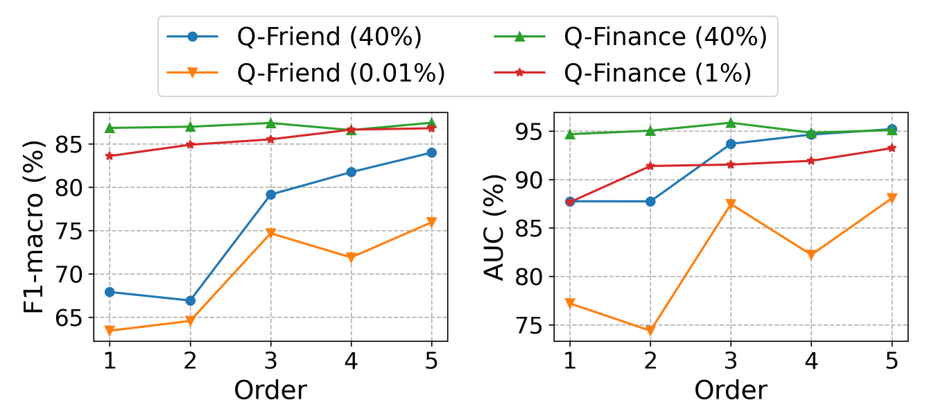
Figure 5: The performance of BWGNN on T-Finance and T-Social with different order $C$.

4.3 Sensitivity Analysis

The Order $C$ in BWGNN. The order $C$ is a crucial hyper-parameter in BWGNN, as Beta wavelet is a $C$-order polynomial of $L$ and is localized in $C$-hops of each node according to proposition 5. Figure 5 presents the F1-macro and AUC scores of BWGNN on two datasets when varying $C$ from 1 to 5. On T-Social, higher $C$ leads to better performances, while on T-Finance, there are no significant differences in results for $C\geq 2$. One possible reason is that the graph in T-Social is much more sparse than that in T-Finance according to Table 1. Thus, a larger range of neighborhoods is required for T-Social.

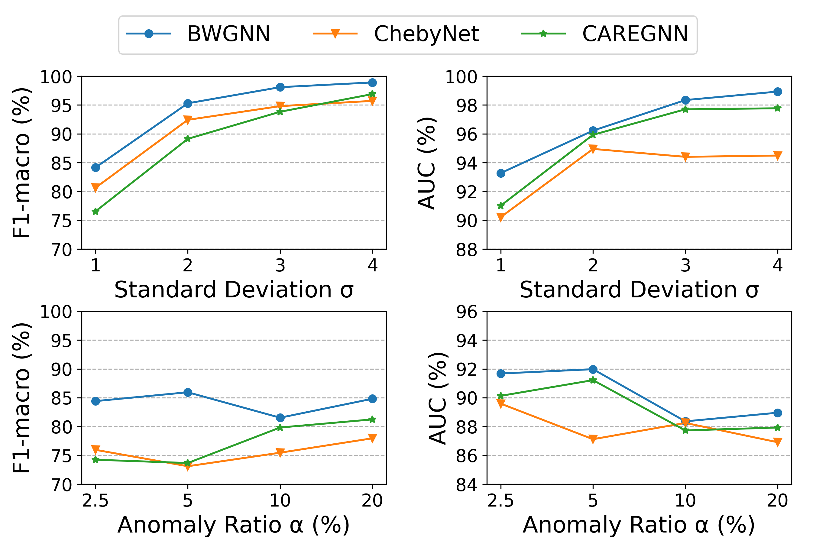
Figure 6: Comparison of performance on T-Finance (1%) with different anomaly degrees controlled by $\sigma$ and $\alpha$.

Impact of Anomaly Degree. We evaluate the effect of different anomaly degrees on ChebyNet, CAREGNN and our BWGNN using the T-Finance dataset. We consider two variables in Section 2.2, including the standard deviation $\sigma$ and the fraction $\alpha$ of the anomalies. We keep the mean value and scale the $\sigma$ of anomalous node features. To control $\alpha$, we follow the attribute perturbation schema in (Ding et al., 2019). We generate different fractions of anomalies by replacing normal node attributes with anomalous ones.

Figure 6 compares the F1-macro and AUC scores of BWGNN, ChebyNet, and CAREGNN on T-Finance (1%) with different anomaly degrees. When $\sigma$ increases, all three models perform better as the anomalies are more distinguishable. Among them, BWGNN is the fastest-growing method and reaches 99% F1-macro at $\sigma=4$. When varying $\alpha$, BWGNN consistently outperforms other methods and is robust to different anomaly degrees.

5 Conclusion

This work presents a novel analysis of graph anomalies in the spectral domain. We find that graph anomalies lead to the ‘right-shift’ phenomenon of spectral energy distributions and further rigorously justify the observation on a vanilla probabilistic model. Inspired by this fact, we propose Beta Wavelet Graph Neural network (BWGNN) to better capture anomaly information on graph. BWGNN leverages Beta graph wavelet to generate band-pass filters with good locality in spectral and spatial domains. Empirical results on four datasets show the superiority and scalability of our model.

Appendix A Proof of Proposition 2

Proof.

By the rotation invariance of Gaussian distributions,

$$\bm{x}\sim\mathcal{N}(\mu e_{N},\sigma^{2}\bm{I}_{N})\Rightarrow\bm{\hat{x}}=\bm{U}^{T}\bm{x}\sim\mathcal{N}(\mu\bm{U}^{T}e_{N},\sigma^{2}\bm{I}_{N}).$$

As the all-the-one vector is the eigenvector for $\lambda_{1}=0$, we have $\hat{x}_{1}\sim\mathcal{N}(\mu\sqrt{n},\sigma^{2})$ and $\hat{x}_{i}\sim\mathcal{N}(0,\sigma^{2}),\forall i\neq 1$. For simplicity, we denote $z_{i}=\frac{\hat{x}_{i}}{\sigma}$ then $z_{1}\sim\mathcal{N}(\tfrac{\mu\sqrt{N}}{\sigma},1)$ and $z_{i}\sim\mathcal{N}(0,1),\forall i\neq 1$.

$$\mathbb{E}_{\bm{x}}\left[\frac{1}{\eta_{k}(\bm{x},\bm{L})}\right]-1 =\mathbb{E}\left[\frac{\sum_{i=k+1}^{N}\hat{x}_{i}^{2}}{\sum_{i=1}^{k}\hat{x}_{i}^{2}}\right]$$

$$=\mathbb{E}\left[\frac{\sum_{i=k+1}^{N}z_{i}^{2}}{\sum_{i=1}^{k}z_{i}^{2}}\right]$$

$$=\mathbb{E}\left[\sum_{i=k+1}^{N}z_{i}^{2}\right]\mathbb{E}\left[\frac{1}{\sum_{i=1}^{k}z_{i}^{2}}\right]$$

$$=(N-k)\mathbb{E}\left[\frac{1}{z_{i}^{2}+\sum_{i=2}^{k}z_{i}^{2}}\right].$$

Notice that $\sum_{i=2}^{k}z_{i}^{2}\sim\tilde{\chi}^{2}(k-1)$ follows the chi-square distribution which is also independent with $z_{1}$. Denote $w=\sum_{i=2}^{k}z_{i}^{2}\geq 0$ and $\rho=\frac{\mu\sqrt{n}}{\sigma}$, we have

$$\mathbb{E}_{\bm{x}}\left[\frac{1}{\eta_{k}(\bm{x},\bm{L})}\right]-1 \propto\mathbb{E}_{w}\left[\mathbb{E}_{z_{1}}\left[\frac{1}{z_{1}^{2}+w}\right]\right]$$

$$=\mathbb{E}_{w}\left[\int_{-\infty}^{+\infty}\frac{1}{\sqrt{2\pi}}e^{-\frac{1}{2}(t-\rho)^{2}}\frac{1}{t^{2}+w}dt\right]$$

$$\propto\mathbb{E}_{w}\left[\int_{-\infty}^{+\infty}e^{-\frac{1}{2}(t-\rho)^{2}}\frac{1}{t^{2}+w}dt\right].$$

As $w$ is nonnegative, we just have to focus on the monotonicity of $f(\rho)=\int_{-\infty}^{+\infty}e^{-\frac{1}{2}(t-\rho)^{2}}\frac{1}{t^{2}+w}dt$ with respect to $\rho$. Due to Lemma 6, we can conclude that $f(\rho)$ is log-concave function and the maximum attains at $0$. Hence, the expectation of the inverse of low-frequency energy ratio $\mathbb{E}_{\bm{x}}[1/\eta_{k}(\bm{x},\bm{L})]$ is monotonically increasing with the anomaly degree $\frac{\sigma}{|\mu|}$. ∎

Lemma 6.

If $w$ is nonnegative, $f(\rho)=\int_{-\infty}^{+\infty}e^{-\frac{1}{2}(t-\rho)^{2}}\frac{1}{t^{2}+w}dt$ is a log-concave function and the maximum attains at 0.

Proof.

By the following two log-concave preserving rules, it is not hard to get our result.

• The product of log-concave functions is still a log-concave function.

• If $f:\mathbb{R}^{n}\times\mathbb{R}^{n}\rightarrow\mathbb{R}$ is a log-concave function, then $g(x)=\int f(x,y)dy$ is still a log-concave function.

Combining with the fact that the density function of Gaussian distributions is log-concave, it is easy to get $f(\rho)$ is log-concave. We omitted the details here. The next step is to argue the optimal solution. As $f(\rho)$ is differentiable, we can interchange the partial and integral here, that is,

$$\frac{\partial f(\rho)}{\partial\rho}=\int_{-\infty}^{+\infty}\frac{1}{t^{2}+w}e^{-\frac{1}{2}(t-\rho)^{2}}(t-\rho)dt.$$

Then,

$$\frac{\partial f(\rho)}{\partial\rho}|_{\rho=0} =\int_{0}^{+\infty}\frac{t}{t^{2}+w}e^{-\frac{1}{2}t^{2}}dt+\int_{-\infty}^{0}\frac{t}{t^{2}+w}e^{-\frac{1}{2}t^{2}}dt$$

$$=\int_{0}^{+\infty}\frac{t}{t^{2}+w}e^{-\frac{1}{2}t^{2}}dt+\int_{0}^{+\infty}\frac{-t}{t^{2}+w}e^{-\frac{1}{2}t^{2}}dt=0.$$

∎

Appendix B Proof of Equation (1)

Proof.

Note that we have $\Sigma_{i=1}^{N}\hat{x}_{i}^{2}=\bm{x^{T}x}$ and $\Sigma_{i=1}^{N}\lambda_{i}\hat{x}_{i}^{2}=\bm{x^{T}Lx}$ according to spectral graph theory (Spielman, 2007). The detailed derivation of Equation (1) is:

$$S_{\textnormal{high}}=\int_{0}^{\lambda_{N}}1-f(t)dt=\lambda_{N}-\sum_{i=1}^{N}(\lambda_{i}-\lambda_{i-1})\eta_{i-1}=\sum_{i=1}^{N}\lambda_{i}(\eta_{i}-\eta_{i-1})=\frac{\sum_{i=1}^{N}\lambda_{i}\hat{x}^{2}_{i}}{\sum_{i=1}^{N}\hat{x}_{i}^{2}}=\frac{\bm{x^{T}Lx}}{\bm{x^{T}x}}$$

∎

Appendix C Baselines and Implementation Details

The first group only considers node features without graph relations:

• MLP: a multi-layer perceptron network consisting of two linear layers with activation functions.

• SVM: (Chang & Lin, 2011): a support vector machine with the Radial Basis Function (RBF) kernel.

The second group is general GNN models for node classification:

• GCN (Kipf & Welling, 2017): a graph convolutional network using the first-order approximation of localized spectral filters on graphs.

• ChebyNet (Defferrard et al., 2016): a graph convolutional network which restricts convolution kernel to a Chebyshev polynomial.

• GAT (Veličković et al., 2017): a graph attention network that employs the attention mechanism for neighbor aggregation.

• GIN (Xu et al., 2019b), a GNN model connecting to Weisfeiler-Lehman (WL) graph isomorphism test.

• GraphSAGE (Hamilton et al., 2017): a GNN model based on a fixed sample number of the neighbor nodes.

• GWNN (Xu et al., 2019a): a graph wavelet neural network using heat kernels to generate wavelet transforms.

The third group is state-of-the-art methods for graph-based anomaly detection:

• GraphConsis (Liu et al., 2020): a heterogeneous graph neural network which tackles context, feature and relation inconsistency problem in graph anomaly detection.

• CAREGNN (Dou et al., 2020): a camouflage-resistant GNN which enhances the aggregation process with three unique modules against camouflages and reinforcement learning.

• PC-GNN (Liu et al., 2021b): a GNN-based imbalanced learning method to solve the class imbalance problem in graph-based fraud detection via resampling.

MLP is implemented by PyTorch (Paszke et al., 2019), and SVM is in Scikit-learn (Pedregosa et al., 2011). For GCN, ChebyNet, GAT, and GraphSAGE, we use the implementation of DGL. GWNN is implemented by ourselves since the source code does not support the fast algorithm. For GraphConsis, CAREGNN, and PC-GNN, we use the code provided by the authors. Our model is implemented based on PyTorch and DGL (Wang et al., 2019b). We conduct all the experiments on a high performance computing server running Ubuntu 20.04 with a Intel(R) Xeon(R) Gold 6226R CPU and 64GB memory.

As the first and second groups of baselines are not specifically designed for anomaly detection, they suffer from class imbalance and produce very few positive predictions. For fair comparisons, in training, we use the weighted cross-entropy Equation (4) in BWGNN. In validation, we search for the best binary classification threshold by adjusting it at 0.05 intervals to achieve the best F1-macro.

Appendix D Additional Experimental Results

In Table 4, we report the average value and standard deviation of 10 runs on YelpChi and Amazon.

Table 4: Experimental results (Mean $\pm$ Std.) of compared methods on the YelpChi and Amazon datasets with 1% and 40% training ratios.

Dataset	YelpChi (1%)		YelpChi (40%)		Amazon (1%)		Amazon (40%)
Metric	F1-macro	AUC	F1-macro	AUC	F1-macro	AUC	F1-macro	AUC
MLP	53.90$\pm$0.23	59.83$\pm$0.40	57.57$\pm$0.89	66.52$\pm$1.09	74.68$\pm$1.25	83.62$\pm$1.76	79.17$\pm$1.26	89.80$\pm$1.04
SVM	60.47$\pm$0.24	62.92$\pm$0.92	70.77$\pm$0.01	70.37$\pm$0.04	83.49$\pm$1.39	81.62$\pm$3.53	90.71$\pm$0.04	90.51$\pm$0.07
GCN	52.48$\pm$0.50	54.06$\pm$0.72	54.31$\pm$0.77	56.51$\pm$1.09	67.93$\pm$1.42	82.85$\pm$0.71	67.47$\pm$0.52	83.49$\pm$0.47
ChebyNet	63.13$\pm$0.50	73.48$\pm$0.74	65.72$\pm$0.48	78.19$\pm$0.63	85.74$\pm$1.67	87.60$\pm$0.61	91.94$\pm$0.29	94.64$\pm$0.53
GAT	50.27$\pm$2.31	50.95$\pm$1.39	54.64$\pm$2.19	57.20$\pm$0.24	60.84$\pm$2.47	73.45$\pm$1.26	83.18$\pm$2.91	89.90$\pm$0.95
GIN	57.57$\pm$1.15	64.73$\pm$1.73	62.85$\pm$0.76	74.09$\pm$1.06	68.69$\pm$4.12	78.83$\pm$3.82	69.26$\pm$2.45	80.56$\pm$2.99
GraphSAGE	58.41$\pm$2.12	67.58$\pm$1.69	65.49$\pm$1.84	78.31$\pm$2.14	70.78$\pm$3.85	75.37$\pm$2.49	74.17$\pm$1.37	86.95$\pm$2.74
GWNN	59.10$\pm$6.53	67.16$\pm$11.44	65.29$\pm$6.67	75.32$\pm$8.97	87.01$\pm$1.98	85.37$\pm$2.32	91.00$\pm$0.27	93.19$\pm$2.22
GraphConsis	56.79$\pm$2.72	66.41$\pm$3.41	58.70$\pm$2.00	69.83$\pm$3.02	68.59$\pm$3.41	74.11$\pm$3.53	75.12$\pm$3.25	87.41$\pm$3.34
CAREGNN	62.18$\pm$1.39	75.07$\pm$3.88	63.32$\pm$0.94	76.19$\pm$2.92	68.78$\pm$1.68	88.69$\pm$3.58	86.39$\pm$1.73	90.53$\pm$1.67
PC-GNN	59.82$\pm$1.42	75.47$\pm$0.98	63.00$\pm$2.30	79.87$\pm$0.14	79.86$\pm$5.65	90.40$\pm$2.05	89.56$\pm$0.77	95.86$\pm$0.14
BWGNN (Homo)	61.15$\pm$0.41	72.01$\pm$0.48	71.00$\pm$0.91	84.03$\pm$0.98	90.92$\pm$0.78	89.45$\pm$0.33	92.29$\pm$0.44	98.06$\pm$0.45
BWGNN (Hetero)	67.02$\pm$0.50	76.95$\pm$1.38	76.96$\pm$0.89	90.54$\pm$0.49	83.83$\pm$3.79	86.59$\pm$2.62	91.72$\pm$0.84	97.42$\pm$0.48

References

- Amar et al. (2005) Amar, C. B., Zaied, M., and Alimi, A. Beta wavelets. synthesis and application to lossy image compression. Advances in Engineering Software, 36(7):459–474, 2005.
- Balcilar et al. (2020) Balcilar, M., Renton, G., Héroux, P., Gaüzère, B., Adam, S., and Honeine, P. Analyzing the expressive power of graph neural networks in a spectral perspective. In ICLR, 2020.
- Bandyopadhyay et al. (2019) Bandyopadhyay, S., Lokesh, N., and Murty, M. N. Outlier aware network embedding for attributed networks. In AAAI, 2019.
- Bao et al. (2019) Bao, Y., Tang, Z., Li, H., and Zhang, Y. Computer vision and deep learning–based data anomaly detection method for structural health monitoring. Structural Health Monitoring, 18(2):401–421, 2019.
- Bedeian & Mossholder (2000) Bedeian, A. G. and Mossholder, K. W. On the use of the coefficient of variation as a measure of diversity. Organizational Research Methods, 3(3):285–297, 2000.
- Bo et al. (2021) Bo, D., Wang, X., Shi, C., and Shen, H. Beyond low-frequency information in graph convolutional networks. In AAAI, 2021.
- Chang & Lin (2011) Chang, C.-C. and Lin, C.-J. Libsvm: a library for support vector machines. ACM transactions on intelligent systems and technology (TIST), 2(3):1–27, 2011.
- Coifman & Maggioni (2006) Coifman, R. R. and Maggioni, M. Diffusion wavelets. Applied and computational harmonic analysis, 21(1):53–94, 2006.
- Cui et al. (2020) Cui, L., Seo, H., Tabar, M., Ma, F., Wang, S., and Lee, D. Deterrent: Knowledge guided graph attention network for detecting healthcare misinformation. In KDD, pp. 492–502, 2020.
- Davis & Goadrich (2006) Davis, J. and Goadrich, M. The relationship between precision-recall and roc curves. In ICML, pp. 233–240, 2006.
- De Oliveira & De Araújo (2015) De Oliveira, H. and De Araújo, G. Compactly supported one-cyclic wavelets derived from beta distributions. arXiv:1502.02166, 2015.
- Defferrard et al. (2016) Defferrard, M., Bresson, X., and Vandergheynst, P. Convolutional neural networks on graphs with fast localized spectral filtering. NeurIPS, pp. 3844–3852, 2016.
- Ding et al. (2019) Ding, K., Li, J., Bhanushali, R., and Liu, H. Deep anomaly detection on attributed networks. In ICDM. SIAM, 2019.
- Dong et al. (2021) Dong, Y., Ding, K., Jalaian, B., Ji, S., and Li, J. Adagnn: Graph neural networks with adaptive frequency response filter. In CIKM, pp. 392–401, 2021.
- Donnat et al. (2018) Donnat, C., Zitnik, M., Hallac, D., and Leskovec, J. Learning structural node embeddings via diffusion wavelets. In KDD, 2018.
- Dou et al. (2020) Dou, Y., Liu, Z., Sun, L., Deng, Y., Peng, H., and Yu, P. S. Enhancing graph neural network-based fraud detectors against camouflaged fraudsters. In CIKM, pp. 315–324, 2020.
- ElAdel et al. (2016) ElAdel, A., Zaied, M., and Amar, C. B. Fast beta wavelet network-based feature extraction for image copy detection. Neurocomputing, 173:306–316, 2016.
- Gama et al. (2019) Gama, F., Ribeiro, A., and Bruna, J. Diffusion scattering transforms on graphs. In ICLR, 2019.
- Grubbs (1969) Grubbs, F. E. Procedures for detecting outlying observations in samples. Technometrics, 11(1):1–21, 1969.
- Hamilton et al. (2017) Hamilton, W. L., Ying, R., and Leskovec, J. Inductive representation learning on large graphs. In NeurIPS, pp. 1025–1035, 2017.
- Hammond et al. (2011) Hammond, D. K., Vandergheynst, P., and Gribonval, R. Wavelets on graphs via spectral graph theory. Applied and Computational Harmonic Analysis, 30(2):129–150, 2011.
- Han et al. (2011) Han, J., Kamber, M., and Pei, J. Data Mining: Concepts and Techniques, 3rd edition. Morgan Kaufmann, 2011.
- He et al. (2021) He, M., Wei, Z., Huang, Z., and Xu, H. Bernnet: Learning arbitrary graph spectral filters via bernstein approximation. NeurIPS, 2021.
- Jemai et al. (2010) Jemai, O., Zaied, M., Amar, C. B., and Alimi, A. M. Fbwn: An architecture of fast beta wavelet networks for image classification. In IJCNN, pp. 1–8. IEEE, 2010.
- Kendall et al. (1946) Kendall, M. G. et al. The advanced theory of statistics. The advanced theory of statistics., 1946.
- Kipf & Welling (2017) Kipf, T. N. and Welling, M. Semi-supervised classification with graph convolutional networks. In ICLR, 2017.
- Kumar et al. (2018) Kumar, S., Hooi, B., Makhija, D., Kumar, M., Faloutsos, C., and Subrahmanian, V. Rev2: Fraudulent user prediction in rating platforms. In WSDM, pp. 333–341, 2018.
- Levie et al. (2018) Levie, R., Monti, F., Bresson, X., and Bronstein, M. M. Cayleynets: Graph convolutional neural networks with complex rational spectral filters. IEEE Transactions on Signal Processing, 67(1):97–109, 2018.
- Li et al. (2021) Li, J., Li, J., Liu, Y., Yu, J., Li, Y., and Cheng, H. Deconvolutional networks on graph data. In NeurIPS, volume 34, pp. 21019–21030, 2021.
- Li et al. (2018) Li, Q., Han, Z., and Wu, X. Deeper insights into graph convolutional networks for semi-supervised learning. In AAAI, pp. 3538–3545, 2018.
- Liu et al. (2021a) Liu, C., Sun, L., Ao, X., Feng, J., He, Q., and Yang, H. Intention-aware heterogeneous graph attention networks for fraud transactions detection. In KDD, pp. 3280–3288, 2021a.
- Liu et al. (2021b) Liu, Y., Ao, X., Qin, Z., Chi, J., Feng, J., Yang, H., and He, Q. Pick and choose: A gnn-based imbalanced learning approach for fraud detection. In Proceedings of the Web Conference 2021, pp. 3168–3177, 2021b.
- Liu et al. (2020) Liu, Z., Dou, Y., Yu, P. S., Deng, Y., and Peng, H. Alleviating the inconsistency problem of applying graph neural network to fraud detection. In SIGIR, pp. 1569–1572, 2020.
- Ma et al. (2021) Ma, X., Wu, J., Xue, S., Yang, J., Zhou, C., Sheng, Q. Z., Xiong, H., and Akoglu, L. A comprehensive survey on graph anomaly detection with deep learning. IEEE Transactions on Knowledge and Data Engineering, 2021.
- McAuley & Leskovec (2013) McAuley, J. J. and Leskovec, J. From amateurs to connoisseurs: modeling the evolution of user expertise through online reviews. In WWW, pp. 897–908, 2013.
- Min et al. (2020) Min, Y., Wenkel, F., and Wolf, G. Scattering GCN: overcoming oversmoothness in graph convolutional networks. In NeurIPS, 2020.
- Min et al. (2021) Min, Y., Wenkel, F., and Wolf, G. Geometric scattering attention networks. In ICASSP, 2021.
- Ngai et al. (2011) Ngai, E. W., Hu, Y., Wong, Y. H., Chen, Y., and Sun, X. The application of data mining techniques in financial fraud detection: A classification framework and an academic review of literature. Decision support systems, 50(3):559–569, 2011.
- Noble & Cook (2003) Noble, C. C. and Cook, D. J. Graph-based anomaly detection. In KDD, pp. 631–636, 2003.
- Nt & Maehara (2019) Nt, H. and Maehara, T. Revisiting graph neural networks: All we have is low-pass filters. arXiv:1905.09550, 2019.
- Paszke et al. (2019) Paszke, A., Gross, S., Massa, F., Lerer, A., Bradbury, J., Chanan, G., Killeen, T., Lin, Z., Gimelshein, N., Antiga, L., et al. Pytorch: An imperative style, high-performance deep learning library. NeurIPS, 32:8026–8037, 2019.
- Pedregosa et al. (2011) Pedregosa, F., Varoquaux, G., Gramfort, A., Michel, V., Thirion, B., Grisel, O., Blondel, M., Prettenhofer, P., Weiss, R., Dubourg, V., et al. Scikit-learn: Machine learning in python. the Journal of machine Learning research, 12:2825–2830, 2011.
- Perraudin et al. (2014) Perraudin, N., Paratte, J., Shuman, D., Martin, L., Kalofolias, V., Vandergheynst, P., and Hammond, D. K. Gspbox: A toolbox for signal processing on graphs. arXiv preprint arXiv:1408.5781, 2014.
- Rayana & Akoglu (2015) Rayana, S. and Akoglu, L. Collective opinion spam detection: Bridging review networks and metadata. In KDD, pp. 985–994, 2015.
- Sipple (2020) Sipple, J. Interpretable, multidimensional, multimodal anomaly detection with negative sampling for detection of device failure. In ICML, pp. 9016–9025. PMLR, 2020.
- Spielman (2007) Spielman, D. A. Spectral graph theory and its applications. In 48th Annual IEEE Symposium on Foundations of Computer Science (FOCS’07), pp. 29–38. IEEE, 2007.
- Ten et al. (2011) Ten, C.-W., Hong, J., and Liu, C.-C. Anomaly detection for cybersecurity of the substations. IEEE Transactions on Smart Grid, 2(4):865–873, 2011.
- Veličković et al. (2017) Veličković, P., Cucurull, G., Casanova, A., Romero, A., Lio, P., and Bengio, Y. Graph attention networks. arXiv:1710.10903, 2017.
- Wang et al. (2019a) Wang, D., Lin, J., Cui, P., Jia, Q., Wang, Z., Fang, Y., Yu, Q., Zhou, J., Yang, S., and Qi, Y. A semi-supervised graph attentive network for financial fraud detection. In ICDM, pp. 598–607. IEEE, 2019a.
- Wang et al. (2019b) Wang, M., Zheng, D., Ye, Z., Gan, Q., Li, M., Song, X., Zhou, J., Ma, C., Yu, L., Gai, Y., Xiao, T., He, T., Karypis, G., Li, J., and Zhang, Z. Deep graph library: A graph-centric, highly-performant package for graph neural networks. arXiv:1909.01315, 2019b.
- Wu et al. (2019) Wu, F., Souza, A., Zhang, T., Fifty, C., Yu, T., and Weinberger, K. Simplifying graph convolutional networks. In ICML, pp. 6861–6871, 2019.
- Wu et al. (2021) Wu, Z., Pan, S., Long, G., Jiang, J., and Zhang, C. Beyond low-pass filtering: Graph convolutional networks with automatic filtering. arXiv preprint arXiv:2107.04755, 2021.
- Xu et al. (2019a) Xu, B., Shen, H., Cao, Q., Qiu, Y., and Cheng, X. Graph wavelet neural network. In ICLR, 2019a.
- Xu et al. (2019b) Xu, K., Hu, W., Leskovec, J., and Jegelka, S. How powerful are graph neural networks? ICLR, 2019b.
- Zhao et al. (2020) Zhao, T., Deng, C., Yu, K., Jiang, T., Wang, D., and Jiang, M. Error-bounded graph anomaly loss for gnns. In CIKM, pp. 1873–1882, 2020.
- Zhao et al. (2021) Zhao, T., Jiang, T., Shah, N., and Jiang, M. A synergistic approach for graph anomaly detection with pattern mining and feature learning. IEEE Transactions on Neural Networks and Learning Systems, 2021.