Adaptive proximal gradient methods are universal
without approximation

Abstract

We show that adaptive proximal gradient methods for convex problems are not restricted to traditional Lipschitzian assumptions. Our analysis reveals that a class of linesearch-free methods is still convergent under mere local Hölder gradient continuity, covering in particular continuously differentiable semi-algebraic functions. To mitigate the lack of local Lipschitz continuity, popular approaches revolve around $\varepsilon$-oracles and/or linesearch procedures. In contrast, we exploit plain Hölder inequalities not entailing any approximation, all while retaining the linesearch-free nature of adaptive schemes. Furthermore, we prove full sequence convergence without prior knowledge of local Hölder constants nor of the order of Hölder continuity. In numerical experiments we present comparisons to baseline methods on diverse tasks from machine learning covering both the locally and the globally Hölder setting.

Keywords. Convex minimization $\cdot$ proximal gradient method $\cdot$ universal methods $\cdot$ linesearch-free adaptive methods $\cdot$ local Hölder gradient continuity $\cdot$ first-order methods

AMS subject classifications. 65K05 $\cdot$ 90C06 $\cdot$ 90C25 $\cdot$ 90C30 $\cdot$ 90C47

1 Introduction

We consider composite minimization problems of the form

$$\operatorname*{minimize}_{x\in{}^{n}}\;\varphi(x)\coloneqq f(x)+g(x)$$

where $f:{}^{n}\rightarrow\m@thbbch@rR$ is convex and has locally Hölder continuous gradient of (possibly unknown) order $\nu\in(0,1]$, and $g:{}^{n}\rightarrow\overline{}\m@thbbch@rR$ is proper, lsc, and convex with easy to compute proximal mapping.

The proximal gradient method is the de facto splitting technique for solving the composite problem (1). Under global Lipschitz continuity of ${\nabla}f$, convergence results and complexity bounds are well established. Nevertheless, there exist many applications where such an assumption is not met. Among these are mixtures of maximum likelihood models [14], classification, robust regression [35, 12], compressive sensing [7] and $p$-Laplacian problems on graphs [16], or the subproblems in the power augmented Lagrangian method [24, 32, 21].

Although often linesearch methods are still applicable under this setting, their additional backtracking procedures can be quite costly in practice. In response to this, this work investigates linesearch-free adaptive methods under mere local Hölder continuity of ${\nabla}f$, covering in particular all continuously differentiable semi-algebraic functions.

In the Hölder differentiable setting, a notable approach was introduced in the seminal works [27, 9] that rely on the notion of $\varepsilon$-oracles [9, Def. 1]. The main idea there is to approximate the Hölder smooth term with the squared Euclidean norm, resulting in an approximate descent lemma [27, Lem. 2] that can be leveraged for a linesearch procedure. More specifically, given $\eta\in(0,1)$, some $\gamma_{0}>0$, and an accuracy threshold $\varepsilon>0$, Nesterov’s universal primal gradient (NUPG) method [27] consists of computing

$$x^{k+1}={} \operatorname{prox}_{\gamma_{k+1}g}{\mathopen{}\left(x^{k}-\gamma_{k+1}{\nabla}f(x^{k})\right)\mathclose{}},$$ (1a)

where $$\gamma_{k+1}=2\gamma_{k}\eta^{m_{k}} m_{k}\in\m@thbbch@rN$$ and is the smallest such that

$$f(x^{k+1})\leq{} f(x^{k})+\langle{}{\nabla}f(x^{k}){},{}x^{k+1}-x^{k}{}\rangle+\tfrac{1}{2\gamma_{k+1}}\|x^{k+1}-x^{k}\|^{2}+\tfrac{1}{2}\varepsilon.$$ (1b)

It is clear that $$\varepsilon$$ is a parameter of the algorithm, a fact further illustrated by the convergence rate

$$\varphi(x^{k})-\varphi(x^{\star})\leq{} \tfrac{\varepsilon}{2}+\tfrac{1}{\varepsilon}^{\frac{1-\nu}{1+\nu}}\tfrac{2L_{\nu}^{\frac{2}{1+\nu}}\|x^{0}-x^{\star}\|^{2}}{k+1},$$ (1c)

where $L_{\nu}$ is a modulus of Hölder continuity of the gradient: the coefficient of the $\nicefrac{{1}}{{(k+1)}}$ term becomes arbitrarily large as higher accuracy is demanded $\varepsilon\to 0$. This approach nevertheless allows handling Hölder smooth problems in the same manner as Lipschitz smooth ones and thus implementing classical improvements such as acceleration [27, 17, 13]. Moreover, its implementability has led to algorithms that go beyond the classical forward-backward splitting, such as primal-dual methods [39, 31] and even variational inequalities [34].

In the context of classical majorization-minimization, when the order and the modulo of smoothness are known, the Hölder smoothness inequality itself has been used to generate descent without the aformentioned approximation. Akin to Lipschitz continuity, Hölder continuity of ${\nabla}f$ with constant $H$ translates into a descent lemma inequality which, after addition of $g(x)$, yields the upper bound to the cost $\varphi$

$$\varphi(x)\leq f(x^{k})+\langle{}{\nabla}f(x^{k}){},{}x-x^{k}{}\rangle+\tfrac{1}{(1+\nu)\lambda_{{k+1},\nu}}\|x-x^{k}\|^{1+\nu}+g(x),$$ (2)

for any $\lambda_{{k+1},\nu}<1/H$, cf. Item 2. This was considered in [5, 15] in a general Banach space setup as well as in [36, 4] for smooth but possibly nonconvex problems. With $x^{k+1}$ denoting the minimizer of the above majorization model, the first-order optimality condition

$$0\in\partial g(x^{k+1})+{\nabla}f(x^{k})+\tfrac{1}{\lambda_{{k+1},\nu}}\|x^{k+1}-x^{k}\|^{-(1-\nu)}(x^{k+1}-x^{k})$$ (3)

reveals that the resulting iterations are essentially an Euclidean proximal gradient method for a particular stepsize $\gamma_{k+1}\coloneqq\lambda_{{k+1},\nu}\|x^{k+1}-x^{k}\|^{1-\nu}$ that bears an implicit dependence on the future iterate $x^{k+1}$.

Such majorize-minimize paradigm adopts $\lambda_{{k+1},\nu}$ as explicit stepsize parameter, and is thus tied to (the knowledge of) the order of $\nu$ of Hölder differentiability. Instead, we directly derive conditions on the “Euclidean” stepsize $\gamma_{k+1}$ and rather regard $\lambda_{{k+1},\nu}$ as an implicit parameter, crucial to the convergence analysis yet absent in the algorithm. (In contrast to $\lambda_{{k+1},\nu}$, the absence of the subscript $\nu$ in $\gamma_{k+1}$ emphasizes the independence of the Hölder exponent on the Euclidean stepsize; this notational convention will be adopted throughout.)

We also remark that the implicit nature of the inclusion (3) is ubiquitous in algorithms that involve proximal terms of the form $\frac{1}{p}\|x-x^{k}\|^{p}$ for $p>1$, such as the cubic Newton and tensor methods [29, 10, 6] or the high-order proximal point algorithm [24, 30, 32, 21]. Notice further that the Hölder proximal gradient update for non-Euclidean norms as described above differs from performing a “scaled” gradient step followed by a higher-order proximal point step. Instead, that corresponds to the anisotropic proximal gradient method [20] for choosing $\phi(x)=\frac{H}{1+\nu}\|x\|_{1+\nu}^{1+\nu}$.

Our contribution

Our approach departs from and improves upon existing works in the following aspects.

• Through a novel analysis of adaPG^π,r [18], we demonstrate that the class of linesearch-free adaptive methods advanced in [25, 18, 26, 19] are convergent even in the locally Hölder differentiable setting, covering in particular the class of semi-algebraic $C^{1}$ functions.

• Our approach bridges the gap between two fundamental approaches to minimizing Hölder-smooth functions: it is both exact as in [5], in the sense that it does not involve nor depend on any predefined accuracy, and universal akin to the approach in [27], for it does not depend on (nor require the knowledge of) problem data such as the Hölder exponent $\nu$.

• We establish sequential convergence (as opposed to subsequential or approximate cost convergence) with an exact rate

  $$\min_{k\leq K}\varphi(x^{k})-\min\varphi\leq O(\tfrac{1}{(K+1)^{\nu}}).$$ (4)

  Differently from existing analyses that rely on a global lower bound on the stepsizes to infer convergence and an $O(\nicefrac{{1}}{{(K+1)}})$ rate in the case $\nu=1$, we identify a scaling of the stepsizes and a lower bound thereof that enables us to tackle the general $\nu\in(0,1)$ regime.

• In numerical simulations we show that adaPG${}^{\pi,\frac{\pi}{2}}$ performs well on a collection of locally and globally Hölder smooth problems, such as classification with Hölder-smooth SVMs and a $p$-norm version of Lasso. We show that our method performs consistenly better than Nesterov’s universal primal gradient method [27] and in many cases better than its fast variant [27], as well as the recently proposed auto-conditioned fast gradient method [22].

2 Universal, adaptive, without approximation

We consider standard (Euclidean) proximal gradient steps

$$x^{k+1}=\operatorname{prox}_{\gamma_{k+1}g}(x^{k}-\gamma_{k+1}{\nabla}f(x^{k}))$$ (5)

for solving (1) under the following assumptions.

Assumption 2.1.

The following hold in problem (1):

1. $f:{}^{n}\rightarrow\m@thbbch@rR$ is convex and has locally Hölder continuous gradient of (possibly unknown) order $\nu\in(0,1]$.

2. $g:{}^{n}\rightarrow\overline{}\m@thbbch@rR$ is proper, lsc, and convex.

3. A solution exists: $\operatorname*{arg\,min}\varphi\neq\emptyset$.

We build upon a series of adaptive algorithms, starting with a pioneering gradient method in [25] and the follow-up studies [18, 26, 19, 40] which contribute with proximal extensions, larger stepsizes, and tighter convergence rate estimates. While standard results of proximal algorithms guarantee a descent along the iterates in terms of the cost, distance to solutions, and fixed-point residual individually, the key idea behind this class of methods is to eliminate linesearch procedures by implicitly ensuring a descent on a (time-varying) combination of the three (see Section 3.1). This was achieved under local Lipschitz continuity of ${\nabla}f$, by exploiting local Lipschitz estimates at consecutive iterates $x^{k-1},x^{k}\in{}^{n}$ generated by the algorithm such as

$$\ell_{k}\coloneqq\frac{\langle{}x^{k}-x^{k-1}{},{}{\nabla}f(x^{k})-{\nabla}f(x^{k-1}){}\rangle}{\|x^{k}-x^{k-1}\|^{2}}$$ (6a)

and

$$L_{k}\coloneqq\frac{\|{\nabla}f(x^{k})-{\nabla}f(x^{k-1})\|}{\|x^{k}-x^{k-1}\|}$$ (6b)

(with the convention $\frac{0}{0}=0$).

Under the assumption considered in the aforementioned references of local Lipschitz continuity of ${\nabla}f$, that is, with $\nu=1$, the estimates $\ell_{k}$ and $L_{k}$ as in (6) remain bounded whenever $x^{k}$ and $x^{k-1}$ range in a bounded set. Although this is no more the case in the setting investigated here, for $\ell_{k}$ and $L_{k}$ may diverge as $x^{k}$ and $x^{k-1}$ get arbitrarily close, we show that these Lipschitz estimates can still be employed even if ${\nabla}f$ is merely locally Hölder continuous.

Specifically, we will consider the following stepsize update rule

$$\textstyle\gamma_{k+1}=\gamma_{k}\min\Biggl{\{}{}\sqrt{\frac{1}{\pi}+\frac{\gamma_{k}}{\gamma_{k-1}}},\leavevmode\nobreak\ \sqrt{\frac{1}{2{\mathopen{}\left[\gamma_{k}^{2}L_{k}^{2}-(2-\pi)\gamma_{k}\ell_{k}-(\pi-1)\right]\mathclose{}}_{+}}}\Biggr{\}}$$ (7)

for some $\pi\in[1,2]$, where $[{}\cdot{}]_{+}\coloneqq\max{\mathopen{}\left\{{}\cdot{},0{}\mathrel{\mid}{}{}\right\}\mathclose{}}$. This correponds to the update rule of the algorithm adaPG^π,r of [18] specialized to the choice $r=\nicefrac{{\pi}}{{2}}$ for the second parameter. This restriction is nevertheless general enough to recover the update rules of [25, Alg. 1], [19, Alg. 2.1], and [26, Alg. 1] ($\pi=1$), as well as the one of [26, Alg. 3] ($\pi=\nicefrac{{3}}{{2}}$), see [19, Rem. 2.4]. In particular, our analysis in the generality of $\pi\in[1,2]$ demonstrates that all these adaptive algorithms are convergent in the locally Hölder (convex) setting.

A crucial challenge in the locally Hölder setting is the lack of a positive uniform lower bound for the stepsize sequence $(\gamma_{k})_{k\in\m@thbbch@rN}$ generated by (7). To mitigate this, we factorize $\gamma_{k}$ as

$$\gamma_{k}=\lambda_{{k},\nu}\|x^{k}-x^{k-1}\|^{1-\nu},$$ (8)

introducing scaled stepsizes $\lambda_{{k},\nu}$ as suggested by the upper bound minimization procedure (3). This allows us to normalize the Hölder inequalities into Lipschitz-like ones, see Section 2.1. (Throughout, the subscript $\nu$ shall be used for quantities with dependence on $\nu$ for clarity of exposition.) Our analysis relies on showing that this scaled stepsize is lower bounded whenever the second term in (7) is active (see Section 3.2). We emphasize that this quantity, while crucial in our convergence analysis, does not appear in the algorithm, which only uses the estimates (6) and the update rule (7), neither of which depend on (the knowledge of) the local Hölder order $\nu$.

The adaptive update (7) allows the stepsize to increase along the iterates, thus distinguishing it from the well-established and popular approach put forward in [11], and followed by many extensions (see for instance recent works by [23, 38, 8], among others), which however can tackle more general problems.

2.1 Hölder continuity estimates

In this section, we set up some basic facts about Hölder continuity of ${\nabla}f$ that will be essential in our analysis. We again emphasize that our convergence analysis makes mere use of existence of $\nu\in(0,1]$ (see Assumption 1), but the algorithm is independent of (the knowledge of) this exponent, cf. adaPG${}^{\pi,\frac{\pi}{2}}$ (Algorithm 1).

Local Hölder continuity of ${\nabla}f$ of order $\nu$ (which we shall refer to as local $\nu$-Hölder continuity of ${\nabla}f$ for brevity) amounts to the existence, for every convex and bounded set $\Omega\subset{}^{n}$, of a constant $L_{{\Omega},\nu}>0$ such that

$$\|{\nabla}f(y)-{\nabla}f(x)\|\leq L_{{\Omega},\nu}\|y-x\|^{\nu}\quad\forall x,y\in\Omega.$$

Note that both norms are the standard Euclidean 2-norms. We remark that the limiting case $\nu=0$ amounts to subgradients of $f$ being bounded on bounded sets, that is, to $f$ being merely convex and real valued with no differentiability requirements. Although not covered by our convergence results in Section 3.2, the preliminary lemmas collected in Section 3.1 still remain valid for any real-valued convex $f$. To clearly emphasize this fact, whenever applicable we shall henceforth specify “(possibly with $\nu=0$)” when invoking 2.1; in this case, the notation ${\nabla}f$ shall indicate any subgradient map ${\nabla}f:{}^{n}\rightarrow{}^{n}$ with ${\nabla}f(x)\in\partial f(x)$, and

$$L_{{\Omega},0}\leq 2\operatorname{lip}_{\Omega}f$$ (9)

is bounded by twice the Lipschitz modulus for $f$ on $\Omega$ [33, Thm. 24.7].

Throughout, we will make use of the following inequalities, which reduce to well-known Lipschitz and cocoercivity properties of ${\nabla}f$ when $\nu=1$. The proof of the second assertion can be found in [36, Lem. 1]; our cocoercivity-like claims are a slight refinement of known global and/or scalar versions, see e.g., [1, Cor. 18.14] and [37, Prop. 1]. The simple proofs of this and the following lemma are provided in the dedicated Section A.

[Hölder-smoothness inequalities]Suppose that $h:{}^{n}\rightarrow\m@thbbch@rR$ is convex and $\nabla{h}$ is $\nu$-Hölder continuous with modulus $L_{{E},\nu}>0$ on a convex set $E\subseteq{}^{n}$ for some $\nu\in[0,1]$. Then, for every $x,y\in{E}$ the following hold:

1. $\langle{}x-y{},{}\nabla{{h}}(x)-\nabla{h}(y){}\rangle\leq L_{{E},\nu}\|x-y\|^{1+\nu}$;

2. ${h}(y)-{h}(x)-\langle{}\nabla{h}(x){},{}y-x{}\rangle\leq\tfrac{L_{{E},\nu}}{1+\nu}\|x-y\|^{1+\nu}$.

If $\nu\neq 0$ and ${\nabla}h$ is $\nu$-Hölder continuous on an enlarged set $\overline{E}\coloneqq E+\operatorname{\overline{B}}(0;\operatorname{diam}E)$ with modulus $L_{{\overline{E}},\nu}$, then the following local cocoercivity-type estimates also hold:

1. $\frac{2\nu}{1+\nu}\frac{1}{L_{{\overline{E}},\nu}^{1\!/\!\nu}}\|{\nabla}h(x)-{\nabla}h(y)\|^{\frac{1+\nu}{\nu}}\leq\langle{}x-y{},{}\nabla{h}(x)-\nabla{h}(y){}\rangle$;

2. $\frac{\nu}{1+\nu}\frac{1}{L_{{\overline{E}},\nu}^{1\!/\!\nu}}\|{\nabla}h(x)-{\nabla}h(y)\|^{\frac{1+\nu}{\nu}}\leq h(y)-h(x)-\langle{}{\nabla}h(x){},{}y-x{}\rangle$.

Algorithm 1 AdaPG${}^{\pi,\frac{\pi}{2}}$: A universal adaptive proximal gradient method

1:starting point $x^{-1}\in{}^{n}$,  stepsizes $\gamma_{0}\geq\gamma_{-1}>0$,  parameter $\pi\in[1,2]$

2:$x^{0}=\operatorname{prox}_{\gamma_{0}g}(x^{-1}-\gamma_{0}{\nabla}f(x^{-1}))$

3:

4:With $\ell_{k},L_{k}$ given in (6), define the stepsize as (with notation $[z]_{+}=\max{\mathopen{}\left\{z,0{}\mathrel{\mid}{}{}\right\}\mathclose{}}$ and convention $\tfrac{1}{0}=\infty$)

$$\gamma_{k+1}=\gamma_{k}\min{\mathopen{}\left\{\sqrt{\frac{1}{\pi}+\frac{\gamma_{k}}{\gamma_{k-1}}},\,\frac{1}{\sqrt{2{\mathopen{}\left[\gamma_{k}^{2}L_{k}^{2}-(2-\pi)\gamma_{k}\ell_{k}+1-\pi\right]\mathclose{}}_{+}}}{}\mathrel{\mid}{}{}\right\}\mathclose{}}$$ (10)

5:$x^{k+1}=\operatorname{prox}_{\gamma_{k+1}g}(x^{k}-\gamma_{k+1}{\nabla}f(x^{k}))$

Based on the inequalities in Section 2.1, given a sequence $(x^{k})_{k\in\m@thbbch@rN}$ we define local estimates of Hölder continuity of ${\nabla}f$ with $\nu\in[0,1]$ as follows:

$$\ell_{{k},\nu}\coloneqq{} \frac{\langle{}x^{k}-x^{k-1}{},{}{\nabla}f(x^{k})-{\nabla}f(x^{k-1}){}\rangle}{\|x^{k}-x^{k-1}\|^{1+\nu}}$$ (11a)

and

$$L_{{k},\nu}\coloneqq{} \frac{\|{\nabla}f(x^{k})-{\nabla}f(x^{k-1})\|}{\|x^{k}-x^{k-1}\|^{\nu}}.$$ (11b)

Let us draw some comments on these quantities. Considering the scaled stepsize $\lambda_{{k},\nu}$ given in (8), it is of immediate verification that

$$\lambda_{{k},\nu}L_{{k},\nu}=\gamma_{k}L_{k},\quad\lambda_{{k},\nu}\ell_{{k},\nu}=\gamma_{k}\ell_{k}.$$ (12)

Moreover, observe that

$$\ell_{{k},\nu}\leq L_{{k},\nu}\leq L_{{\Omega},\nu}$$ (13)

holds whenever $L_{{\Omega},\nu}$ is a $\nu$-Hölder modulus for ${\nabla}f$ on a compact convex set $\Omega$ that contains both $x^{k-1}$ and $x^{k}$, the first inequality following from a simple application of Cauchy-Schwartz. We also remark that defining $\ell_{{k},\nu}$ and $L_{{k},\nu}$ as above in place of a cocoercivity-like estimate

$$c_{{k},\nu}\coloneqq\biggl{(}\frac{2\nu}{1+\nu}\frac{\|{\nabla}f(x^{k})-{\nabla}f(x^{k-1})\|^{1+\frac{1}{\nu}}}{\langle{}x^{k}-x^{k-1}{},{}{\nabla}f(x^{k})-{\nabla}f(x^{k-1}){}\rangle}\biggr{)}^{\nu}$$

causes no loss of generality, since each one among $c_{{k},\nu}$, $\ell_{{k},\nu}$ and $L_{{k},\nu}$ can be derived based on the other two. The use of $\ell_{{k},\nu}$ and $L_{{k},\nu}$ provides nevertheless a simpler and more straightforward Hölder estimate, contrary to $c_{{k},\nu}$ which instead involves counterintuitive powers and coefficients, as well as a potentially looser Hölder modulus, and fails to cover the limiting case $\nu=0$, cf. Item 3.

Let us denote the forward operator by

$$H_{k}\coloneqq{\rm id}-\gamma_{k}{\nabla}f.$$ (14)

The subgradient characterization of the proximal gradient update (5) then reads

$$H_{k}(x^{k-1})-H_{k}(x^{k})\in\gamma_{k}\partial\varphi(x^{k}).$$ (15)

As in [19], the combined use of $\ell_{{k},\nu}$ and $L_{{k},\nu}$ yields a local Hölder modulus for the forward operator, though in this work it will be convenient to express it with respect to the scaled stepsize $\lambda_{{k},\nu}$ as in (8).

Let $\ell_{{k},\nu}$ and $L_{{k},\nu}$ be as in (11) for some $x^{k-1},x^{k}\in{}^{n}$, and let $H_{k}$ be as in (14) for some $\gamma_{k}>0$. Then, for any $\nu\in[0,1]$ and with $\lambda_{{k},\nu}$ as in (8) it holds that

$$M_{k}\coloneqq{} \tfrac{\|H_{k}(x^{k})-H_{k}(x^{k-1})\|^{2}}{\|x^{k}-x^{k-1}\|^{2}}=1+\lambda_{{k},\nu}^{2}L_{{k},\nu}^{2}-2\lambda_{{k},\nu}\ell_{{k},\nu}$$

$$={} 1+\gamma_{k}^{2}L_{k}^{2}-2\gamma_{k}\ell_{k}.$$

Being $M_{k}$ a Lipschitz estimate, unless ${\nabla}f$ is locally Lipschitz continuous there is no guarantee that $M_{k}$ is bounded for pairs $x^{k-1},x^{k}$ ranging in a compact set. The $\nu$-Hölder estimate of the forward operator $H_{k}$, which instead is guaranteed to be bounded on bounded sets (for bounded $(\gamma_{k})_{k\in\m@thbbch@rN}$), is given by

$$M_{{k},\nu}\coloneqq{} M_{k}\|x^{k}-x^{k-1}\|^{1-\nu}=\tfrac{\|H_{k}(x^{k})-H_{k}(x^{k-1})\|}{\|x^{k}-x^{k-1}\|^{\nu}}$$

$$\leq{} (1+\lambda_{{k},\nu}L_{{k},\nu})\|x^{k}-x^{k-1}\|^{1-\nu},$$ (16)

where the inequality follows from the triangle inequality and the definition of $L_{{k},\nu}$, cf. (11b).

3 AdaPG${}^{\pi,\frac{\pi}{2}}$ revisited

In this section adaPG${}^{\pi,\frac{\pi}{2}}$ is presented in Algorithm 1 for solving composite problems (1). The main oracles of the algorithm are plain proximal and gradient evaluations. We refer to [2, §6] for examples of functions with easy to evaluate proximal maps.

AdaPG${}^{\pi,\frac{\pi}{2}}$ incorporates the simple stepsize update rule (10) with a parameter $\pi\in[1,2]$ that strikes a balance between speed of recovery from small values (e.g., due to steep or ill-conditioned regions), and magnitude of the stepsize dictated by the second term. If $\pi=1$, whenever $\gamma_{k}^{2}L_{k}^{2}\leq\gamma_{k}\ell_{k}$, the second term reduces to $\nicefrac{{1}}{{0}}=\infty$, and $\gamma_{k+1}=\gamma_{k}\sqrt{1+\nicefrac{{\gamma_{k}}}{{\gamma_{k-1}}}}$ strictly increases. On the other end of the spectrum, if $\pi=2$ the update reduces to

$$\gamma_{k+1}=\gamma_{k}\min{\mathopen{}\left\{\sqrt{\tfrac{1}{2}+\tfrac{\gamma_{k}}{\gamma_{k-1}}},\,\tfrac{1}{\sqrt{2{\mathopen{}\left[\gamma_{k}^{2}L_{k}^{2}-1\right]\mathclose{}}_{+}}}{}\mathrel{\mid}{}{}\right\}\mathclose{}},$$

where having the first term active (for instance if $\gamma_{k}L_{k}\leq 1$) for two consecutive updates already ensures an increase in the stepsize owing to the simple observation that ${\nicefrac{{1}}{{2}}+\sqrt{\nicefrac{{1}}{{2}}}}>1$.

While adaPG${}^{\pi,\frac{\pi}{2}}$ has the ability to recover from a potentially bad choice of initial stepsizes $\gamma_{0},\gamma_{-1}$, the behavior of the algorithm during the first iterations can be impacted negatively. To eliminate such scenarios, $\gamma_{0}$ can be refined by running offline proximal gradient updates. Specifically, starting from the initial point $x^{-1}$, $\gamma_{0}$ can be updated as the inverse of either one of (11b) or (11a) evaluated between $x^{-1}$ and the obtained point. If the updated stepsize is substantially smaller than the original one, the same procedure may be repeated an additional time. Once a reasonable $\gamma_{0}$ is obtained, we suggest selecting $\gamma_{-1}$ small enough such that $\sqrt{\frac{1}{\pi}+\frac{\gamma_{0}}{\gamma_{-1}}}\geq\frac{1}{\sqrt{2L_{0}}},$ ensuring that $\gamma_{1}$ would be proportional to the inverse of $L_{0}$. We remark that the choice of $\gamma_{-1}$ does not affect the sequential convergence results of Section 3.2. It does nevertheless affect the constant in our sublinear rate results of Section 3.2, through possibly having a larger $\rho_{\rm max}$ therein, although this effect is a mere theoretical technicality with negligible practical implications.

3.1 Preliminary lemmas

This subsection collects some preliminary results adaptated from [25, 18, 26, 19] and that hold true under convexity assumption without further restrictions. All the proofs, although differing only by negligible adaptations, are nevertheless provided in the dedicated Section B to demonstrate their independence of $q\in[0,1]$. In particular, the next lemma can be viewed as a counterpart of the well known firm nonexpansiveness (FNE) of $\operatorname{prox}_{\gamma g}$, which is recovered when $\gamma_{k+1}=\gamma_{k}$, and offers a refinement of the nonexpansiveness-like inequality in [26, Lem. 12] that follows after an application of Cauchy-Schwarz.

[FNE-like inequality]Let Assumptions 1 and 2 hold (possibly with $\nu=0$). For any $\gamma_{k}>0$ and denoting $\rho_{k+1}\coloneqq\nicefrac{{\gamma_{k+1}}}{{\gamma_{k}}}$, iterates (5) satisfy the following:

$$\tfrac{1}{\rho_{k+1}}\|x^{k+1}-x^{k}\|^{2}\leq{} \langle{}H_{k}(x^{k-1})-H_{k}(x^{k}){},{}x^{k}-x^{k+1}{}\rangle$$

$$\leq{} \rho_{k+1}\|H_{k}(x^{k-1})-H_{k}(x^{k})\|^{2}.$$

By combining this inequality with the identity in Section 2.1 we obtain the following.

Let Assumptions 1 and 2 hold (possibly with $\nu=0$). For any $\gamma_{k}>0$, and with $M_{k}$ and $\lambda_{{k},\nu}$ as in (14) and (8), iterates (5) satisfy

$$\|x^{k+1}-x^{k}\|\leq\tfrac{\gamma_{k}}{\gamma_{k+1}}M_{k}\|x^{k-1}-x^{k}\|.$$ (17)

We next present the main descent inequality taken from [19, Lem. 2.2]. Its proof is nevertheless included in the appendix to demonstrate its independence of $\nu$: it relies on mere use of convexity inequalities and identities involving $L_{k},\ell_{k}$ as in Sections 3.1 and 2.1 to express norms and inner products in terms of $\|x^{k}-x^{k-1}\|^{2}$. It reveals that for any $\pi\geq 0$ and $x^{\star}\in\operatorname*{arg\,min}\varphi$, up to a proper stepsize selection, the function

$$\mathcal{U}_{k}^{\pi}(x^{\star})\coloneqq\tfrac{1}{2}\|x^{k}-x^{\star}\|^{2}+\tfrac{1}{2}\|x^{k}-x^{k-1}\|^{2}+\gamma_{k}(1+\pi\rho_{k})P_{k-1}$$ (18)

monotonically decreases, where we introduced the symbol

$$P_{k}\coloneqq\varphi(x^{k})-\min\varphi$$ (19)

for the sake of conciseness.

[main inequality]Let 2.1 hold (possibly with $\nu=0$), and consider a sequence generated by proximal gradient iterations (5) with $\gamma_{k}>0$ and $\rho_{k+1}\coloneqq\nicefrac{{\gamma_{k+1}}}{{\gamma_{k}}}$. Then, for any $\pi\geq 0$, $x^{\star}\in\operatorname*{arg\,min}\varphi$, and $k\geq 1$ the following holds:

$$\mathcal{U}_{k+1}^{\pi}(x^{\star})\leq{} \mathcal{U}_{k}^{\pi}(x^{\star})-\gamma_{k}\bigl{(}1+\pi\rho_{k}-\pi\rho_{k+1}^{2}\bigr{)}P_{k-1}$$

$$-\bigl{\{}\tfrac{1}{2}-\rho_{k+1}^{2}\bigl{[}\gamma_{k}^{2}L_{k}^{2}-\gamma_{k}\ell_{k}(2-\pi)+1-\pi\bigr{]}\bigr{\}}\|x^{k}-x^{k-1}\|^{2}.$$ (20)

Apparently, the stepsize update rule of adaPG${}^{\pi,\frac{\pi}{2}}$ is designed so as to make the coefficients of $P_{k-1}$ and $\|x^{k}-x^{k-1}\|^{2}$ on the right-hand side of (20) negative, so that the corresponding proximal gradient iterates monotonically decrease the value of $\mathcal{U}_{k}^{\pi}(x^{\star})$.

[basic properties of adaPG${}^{\pi,\frac{\pi}{2}}$]Under 2.1 (possibly with $\nu=0$), the following hold for the iterates generated by adaPG${}^{\pi,\frac{\pi}{2}}$:

1. $(\mathcal{U}_{k}^{\pi}(x^{\star}))_{k\in\m@thbbch@rN}$ as defined in (18) decreases and converges to a finite value.

2. The sequence $(x^{k})_{k\in\m@thbbch@rN}$ is bounded and admits at most one optimal limit point.

3. $P_{K}^{\rm min}\leq\mathcal{U}_{1}^{\pi}(x^{\star})\big{/}\bigl{(}\sum_{k=1}^{K+1}\gamma_{k}\bigr{)}$ for every $K\geq 1$, where $P_{k}^{\rm min}\coloneqq\min_{i\leq k}P_{i}$.

The validity of Item 3 also when $\nu=0$ hints that having $\sum_{k\in\m@thbbch@rN}\gamma_{k}=\infty$ suffices to infer convergence results for the proximal subgradient method without differentiability of $f$. Whether, or under which conditions, this is really the case is currently an open problem.

3.2 Convergence and rates

Distinguishing between the iterates in which the stepsize is updated according to the first or the second element in the minimum of (10) will play a fundamental role in our analysis. For this reason, it is convenient to introduce the following notation:

$$K_{1}\coloneqq{} {\mathopen{}\left\{k\in\m@thbbch@rN{}\mathrel{\mid}{}\gamma_{k+1}=\gamma_{k}\sqrt{\tfrac{1}{\pi}+\tfrac{\gamma_{k}}{\gamma_{k-1}}}\right\}\mathclose{}}$$ (21a)

and

$$K_{2}\coloneqq{} \m@thbbch@rN\setminus K_{1}.$$ (21b)

Unlike its locally Lipschitz counterpart ($\nu=1$), in the Hölder setting, a global lower bound for the stepsize sequence $(\gamma_{k})_{k\in\m@thbbch@rN}$ cannot be expected. Nevertheless, a lower bound for the scaled stepsizes $\lambda_{{k},\nu}$ whenever $k\in K_{2}$ is sufficient to ensure convergence.

Let 2.1 hold (possibly with $\nu=0$), and consider the iterates generated by adaPG${}^{\pi,\frac{\pi}{2}}$. Then, with $K_{2}$ as in (21b), for every $k\in K_{2}$

$$\lambda_{{k},\nu}\geq\frac{1}{\sqrt{2}L_{{k},\nu}\rho_{\rm max}}\leavevmode\nobreak\ \leavevmode\nobreak\ \text{and}\leavevmode\nobreak\ \leavevmode\nobreak\ \rho_{k+1}\geq\tfrac{1}{\sqrt{2}\lambda_{{k},\nu}L_{{k},\nu}},$$ (22)

where $\rho_{\rm max}\coloneqq\max{\mathopen{}\left\{\frac{1}{2}\bigl{(}1+\sqrt{1+\nicefrac{{4}}{{\pi}}}\bigr{)},\frac{\gamma_{0}}{\gamma_{-1}}{}\mathrel{\mid}{}{}\right\}\mathclose{}}$.

Proof.

Owing to $\rho_{k+1}\leq\sqrt{\nicefrac{{1}}{{\pi}}+\rho_{k}}$ as ensured in (4), it can be verified with a trivial induction argument that

$$\rho_{k}\leq\rho_{\rm max}\coloneqq\max{\mathopen{}\left\{\tfrac{1}{2}(1+\sqrt{1+\nicefrac{{4}}{{\pi}}}),\rho_{0}{}\mathrel{\mid}{}{}\right\}\mathclose{}}\quad\text{for all }k\geq 0.$$ (23)

If $k\in K_{2}$, then $\gamma_{k+1}$ coincides with the second update in (10), and thus

$$\rho_{\rm max}\geq\rho_{k+1}=\frac{1}{\sqrt{2{\mathopen{}\left[\lambda_{{k},\nu}^{2}L_{{k},\nu}^{2}-(2-\pi)\lambda_{{k},\nu}\ell_{{k},\nu}+1-\pi\right]\mathclose{}}_{+}}}\geq\frac{1}{\sqrt{2}\lambda_{{k},\nu}L_{{k},\nu}},$$ (24)

completing the proof. ∎

The anticipated lower bound on $(\lambda_{{k},\nu})_{k\in K_{2}}$ will follow from (13), once boundedness of the sequence $(x^{k})_{k\in\m@thbbch@rN}$ generated by adaPG${}^{\pi,\frac{\pi}{2}}$ is established.

In our convergence analysis we will need the following lemma that extends [18, Lem. B.2] by allowing a vanishing stepsize. As a result it is only $\gamma_{k+1}$ times the cost that can be ensured to converge to zero, which will nevertheless prove sufficient for our convergence analysis in the proof of Section 3.2.

Suppose that a sequence $(x^{k})_{k\in\m@thbbch@rN}$ converges to an optimal point $x^{\star}\in\operatorname*{arg\,min}\varphi$, and for every $k$ let $\bar{x}^{k}\coloneqq\operatorname{prox}_{\gamma_{k+1}g}(x^{k}-\gamma_{k+1}{\nabla}f(x^{k}))$ with $(\gamma_{k})_{k\in\m@thbbch@rN}\subset{}_{++}$ bounded. Then, $(\bar{x}^{k})_{k\in\m@thbbch@rN}$ too converges to $x^{\star}$ and $(\gamma_{k+1}(\varphi(\bar{x}^{k})-\min\varphi))_{k\in\m@thbbch@rN}\to 0$.

Proof.

By nonexpansiveness of the proximal mapping

$$\|\bar{x}^{k}-x^{\star}\|\leq\|x^{k}-x^{\star}-\gamma_{k+1}({\nabla}f(x^{k})-{\nabla}f(x^{\star}))\|\leq\|x^{k}-x^{\star}\|+\gamma_{k+1}\|{\nabla}f(x^{k})-{\nabla}f(x^{\star})\|\to 0,$$

where we used the fact that $x^{\star}=\operatorname{prox}_{\gamma_{k+1}g}(x^{\star}-\gamma_{k+1}{\nabla}f(x^{\star}))$ for any $\gamma_{k+1}>0$ in the first inequality, and boundedness of $\gamma_{k+1}$ in the last implication. Moreover, for every $k\in\m@thbbch@rN$ one has

$$\gamma_{k+1}(\varphi(\bar{x}^{k})-\min\varphi)=\gamma_{k+1}(f(\bar{x}^{k})+g(\bar{x}^{k})-\min\varphi)\leq\gamma_{k+1}(f(\bar{x}^{k})-f(x^{\star}))-\langle x^{k}-\gamma_{k+1}{\nabla}f(x^{k})-\bar{x}^{k},x^{\star}-\bar{x}^{k}\rangle,$$

where in the inequality subgradient characterization of proximal mapping. The inner product vanishes since both $x^{k}$ and $\bar{x}^{k}$ converge to $x^{\star}$, and the claim follows by continuity of $f$ and lower semicontinuity of $\varphi$. ∎

[convergence]Under 2.1, the sequence $(x^{k})_{k\in\m@thbbch@rN}$ generated by adaPG${}^{\pi,\frac{\pi}{2}}$ converges to some $x^{\star}\in\operatorname*{arg\,min}\varphi$.

Proof.

We first show two intermediate claims.

1. If $\nu>0$, then $\operatorname*{inf}_{k\in\m@thbbch@rN}P_{k}=0$, and in particular $(x^{k})_{k\in\m@thbbch@rN}$ admits a (unique) optimal limit point.

   If $\sup_{k\in\m@thbbch@rN}\gamma_{k}=\infty$, then we know from Item 3 that $\liminf_{k\to\infty}P_{k}=0$. Suppose instead that $(\gamma_{k})_{k\in\m@thbbch@rN}$ is bounded. Then, the set $K_{2}$ as in (21b) must be infinite. Since $L_{{k},\nu}\leq L_{{\Omega},\nu}$, it follows from Section 3.2 that

   $$\lambda_{{k},\nu}\geq\lambda_{{\rm min},\nu}\coloneqq\frac{1}{\sqrt{2}L_{{\Omega},\nu}\rho_{\rm max}}\quad\forall k\in K_{2},$$ (25)

   hence from (45) that

   $$\sum_{k\in K_{2}}\|x^{k}-x^{k-1}\|^{1-\nu}(1+\pi\rho_{k}-\pi\rho_{k+1}^{2})P_{k-1}<\infty.$$

   Noticing that $1+\pi\rho_{k}-\pi\rho_{k+1}^{2}=0$ for $k\notin K_{2}$, necessarily $1+\pi\rho_{k}-\pi\rho_{k+1}^{2}\not\to 0$ as $K_{2}\ni k\to\infty$ (or, equivalently, as $k\to\infty$), for otherwise $\liminf_{k\to\infty}\rho_{k}>1$ and thus $\gamma_{k}\nearrow\infty$. Therefore, there exists an infinite set $\tilde{K}_{2}\subseteq K_{2}$ such that $1+\pi\rho_{k}-\pi\rho_{k+1}^{2}\geq\varepsilon>0$ for all $k\in\tilde{K}_{2}$, implying that

   $$\sum_{k\in\tilde{K}_{2}}\|x^{k}-x^{k-1}\|^{1-\nu}P_{k-1}<\infty.$$

   Thus, $\lim_{\tilde{K}_{2}\ni k\to\infty}\|x^{k}-x^{k-1}\|=0$ (or $\liminf_{k\in\tilde{K}_{2}}P_{k-1}=0$, in which case there is nothing to show). For any $x^{\star}\in\operatorname*{arg\,min}\varphi$ we thus have

   $$0\leq P_{k}=\varphi(x^{k})-\min\varphi\leq{} \langle{}x^{k}-x^{\star}{},{}\tfrac{x^{k-1}-x^{k}}{\gamma_{k}}-\bigl{(}{\nabla}f(x^{k-1})-{\nabla}f(x^{k})\bigr{)}{}\rangle$$

   $$\leq{} \|x^{k}-x^{\star}\|{\mathopen{}\left(\tfrac{1}{\gamma_{k}}\|x^{k-1}-x^{k}\|+\|{\nabla}f(x^{k-1})-{\nabla}f(x^{k})\|\right)\mathclose{}}$$ (26)

   $$={} \|x^{k}-x^{\star}\|{\mathopen{}\left(\tfrac{1}{\lambda_{{k},\nu}\|x^{k-1}-x^{k}\|^{1-\nu}}\|x^{k-1}-x^{k}\|+L_{{k},\nu}\|x^{k-1}-x^{k}\|^{\nu}\right)\mathclose{}}$$

   $$\leq{} \|x^{k}-x^{\star}\|\|x^{k-1}-x^{k}\|^{\nu}{\mathopen{}\left(\tfrac{1}{\lambda_{{\rm min},\nu}}+L_{{\Omega},\nu}\right)\mathclose{}}\quad\forall k\in\tilde{K}_{2}.$$

   Since $\nu>0$, by taking the limit as $\tilde{K}_{2}\ni k\to\infty$ we obtain that $\lim_{\tilde{K}_{2}\ni k\to\infty}P_{k}=0$.

2. If $\nu>0$ and $(\gamma_{k})_{k\in\m@thbbch@rN}$ is bounded, then $(x^{k})_{k\in\m@thbbch@rN}$ converges to a solution.

   Suppose first that $(\gamma_{k})_{k\in\m@thbbch@rN}$ is bounded. Consider a subsequence $(x^{k})_{k\in K}$ such that $\lim_{K\ni k\to\infty}P_{k}=0$, which exists and converges to a solution $x^{\star}$ by Claim thm:convergence(a). Since $(\gamma_{k})_{k\in\m@thbbch@rN}$ is bounded, in light of Section 3.2 also $x^{k+1}\to x^{\star}$ and, in turn, $x^{k+2}\to x^{\star}$ as well. Then,

   $$\mathcal{U}_{k+1}^{\pi}(x^{\star})=\tfrac{1}{2}\|x^{k+1}-x^{\star}\|^{2}+\tfrac{1}{2}\|x^{k+1}-x^{k}\|^{2}+\gamma_{k}{\mathopen{}\left(1+\pi\rho_{k+1}\right)\mathclose{}}P_{k}\to 0\quad\text{as }K\ni k\to\infty,$$

   and thus $\frac{1}{2}\|x^{k}-x^{\star}\|\leq\mathcal{U}_{k}^{\pi}(x^{\star})\to 0$ as $k\to\infty$, since the entire sequence $(\mathcal{U}_{k}^{\pi}(x^{\star}))_{k\in\m@thbbch@rN}$ is convergent.

To conclude the proof of the theorem, it remains to show that also in case $(\gamma_{k})_{k\in\m@thbbch@rN}$ is unbounded the sequence $(x^{k})_{k\in\m@thbbch@rN}$ converges to a solution. To this end, let us suppose now that $\gamma_{k}$ is not bounded. This case requires requires a few more technical steps, which can nevertheless almost verbatim be adaptated from the proof of [19, Thm. 2.4(ii)]; we emphasize that the difference here is that the stepsize sequence is not guaranteed to be bounded away from zero.

We start by observing that Claim thm:convergence(a) and Item 2 ensure that an optimal limit point $x^{\star}\in\operatorname*{arg\,min}\varphi$ exists. It then suffices to show that $\mathcal{U}_{k}^{\pi}(x^{\star})$ converges to zero. To arrive to a contradiction, suppose that this is not the case, that is, that $U\coloneqq\lim_{k\to\infty}\mathcal{U}_{k}^{\pi}(x^{\star})>0$. We shall henceforth proceed by intermediate claims that follow from this condition, eventually arriving to a contradictory conclusion.

1. For any $K\subseteq\m@thbbch@rN$, $\lim_{K\ni k\to\infty}x^{k}=x^{\star}$ holds iff $\lim_{K\ni k\to\infty}\gamma_{k+1}=\infty$.

   The implication “$\Leftarrow$” follows from

   $$\gamma_{k}P_{k-1}\leq\mathcal{U}_{k}^{\pi}(x^{\star})<\infty$$

   since $(x^{k})_{k\in\m@thbbch@rN}$ is bounded and $x^{\star}$ is its unique optimal limit point.

   Suppose now that $(x^{k})_{k\in K}\to x^{\star}$. To arrive to a contradiction, up to possibly extracting suppose that $(\gamma_{k+1})_{k\in K}\to\bar{\gamma}\in[0,\infty)$. Then, it follows from Section 3.2 that $(x^{k+1})_{k\in K}\to x^{\star}$ and $(\gamma_{k+1}P_{k+1})_{k\in K}\to 0$. As shown in (23)

   $$\rho_{k}\leq\rho_{\rm max}\quad\text{for all }k\geq 0$$ (27)

   which in turn implies $(\gamma_{k+2}P_{k+1})_{k\in K}\to 0$ and that $(\gamma_{k+2})_{k\in K}$ is also bounded, we may iterate and infer that also $(x^{k+2})_{k\in K}$ converges to $x^{\star}$. Recalling the definition of $\mathcal{U}_{k}^{\pi}$ in (18),

   $$\mathcal{U}_{k+2}^{\pi}(x^{\star})\coloneqq{} \tfrac{1}{2}\|x^{k+2}-x^{\star}\|^{2}+\tfrac{1}{2}\|x^{k+2}-x^{k+1}\|^{2}+\gamma_{k+2}(1+\pi\rho_{k+2})P_{k+1}\to 0,$$

   contradicting $U=\lim_{K\ni k\to\infty}\mathcal{U}_{k+2}^{\pi}(x^{\star})>0$.

2. Suppose that $(x^{k})_{k\in K}\to x^{\star}$; then also $(x^{k-1})_{k\in K}\to x_{\star}$.

   It follows from the previous claim that $\lim_{K\ni k\to\infty}\gamma_{k+1}=\infty$. Because of (27), one must also have $\lim_{K\ni k\to\infty}\gamma_{k}=\infty$. Invoking again the previous claim, by the arbitrarity of the index set $K$ the assertion follows.

3. Suppose that $(x^{k})_{k\in K}\to x^{\star}$; then $(\gamma_{k-1}L_{k-1})_{k\in K}\to\infty$ and $(\rho_{k})_{k\in K}\to 0$.

   Using the previous claim twice, $x^{k-1},x^{k-2}\to x^{\star}$ as $K\ni k\to\infty$. In particular

   $$\lim_{K\ni k\to\infty}\|x^{k-1}-x^{k-2}\|^{2}=0.$$ (28)

   From the expression (18) of $\mathcal{U}_{k}^{\pi}$ we then have

   $$\lim_{K\ni k\to\infty}\gamma_{k}(1+\pi\rho_{k})P_{k-1}=U,$$ (29)

   where we remind that by contradiction assumption $U\coloneqq\lim_{k\to\infty}\mathcal{U}_{k}^{\pi}(x^{\star})>0$. Denoting $C\coloneqq\rho_{\rm max}(1+\pi\rho_{\rm max})$, we have

   $$\gamma_{k-1}P_{k-1}\leq{} \|x^{k-1}-x^{\star}\|{\mathopen{}\left(\|x^{k-1}-x^{k-2}\|+\gamma_{k-1}\|{\nabla}f(x^{k-1})-{\nabla}f(x^{k-2})\|\right)\mathclose{}}$$

   $$={} \|x^{k-1}-x^{\star}\|{\mathopen{}\left(\|x^{k-1}-x^{k-2}\|+\gamma_{k-1}L_{k-1}\|x^{k-1}-x^{k-2}\|^{\nu}\right)\mathclose{}}$$

   for every $k$. Then, by (29)

   $$0<U={} \lim_{K\ni k\to\infty}\gamma_{k}(1+\pi\rho_{k})P_{k-1}={}\liminf_{K\ni k\to\infty}\rho_{k}(1+\pi\rho_{k})\gamma_{k-1}P_{k-1}$$

   $$\leq{} \rho_{\rm max}(1+\pi\rho_{\rm max})\liminf_{K\ni k\to\infty}\|x^{k-1}-x^{\star}\|{\mathopen{}\left(\|x^{k-1}-x^{k-2}\|+\gamma_{k-1}L_{k-1}\|x^{k-1}-x^{k-2}\|^{\nu}\right)\mathclose{}}$$

   which yields the first claim owing to (28) and $\nu>0$.

   This along with the update rule (10) implies

   $$\rho_{k}\leq\frac{1}{2{\mathopen{}\left[\gamma_{k-1}^{2}L_{k-1}^{2}-(2-\pi)\gamma_{k-1}\ell_{k-1}+1-\pi\right]\mathclose{}}}\to 0,$$

   as claimed.

Having shown the above claims, the proof is concluded as in [18, Thm. 2.4(ii)] by constructing a specific unbounded stepsize sequence and using claims 1^claims*i and 3^claims*i to obtain the sought contradiction. ∎

While a global lower bound for the stepsizes $(\gamma_{k})_{k\in\m@thbbch@rN}$ is not available, it is at the moment unclear whether one for the (entire) scaled sequence $(\lambda_{{k},\nu})_{k\in\m@thbbch@rN}$ exists. Nevertheless, with $P_{k}$ as in (19), a lower bound for an alternative scaled sequence $(\gamma_{k+1}P_{k}^{-\nicefrac{{(1-\nu)}}{{\nu}}})_{k\in\m@thbbch@rN}$ does exist, thanks to which the following convergence rate can be achieved.

[sublinear rate]Suppose that 2.1 holds. Then, the following sublinear rate holds for the iterates generated by adaPG${}^{\pi,\frac{\pi}{2}}$:

$$\min_{k\leq K}P_{k}\leq\max{\mathopen{}\left\{\frac{\mathcal{U}_{1}^{\pi}(x^{\star})}{\gamma_{0}(K+1)},\frac{C(\pi,\nu)\mathcal{U}_{1}^{\pi}(x^{\star})^{\frac{1+\nu}{2}}L_{{\Omega},\nu}}{(K+1)^{\nu}}{}\mathrel{\mid}{}{}\right\}\mathclose{}},$$

where $C(\pi,\nu)=\sqrt{2}{\mathopen{}\left(\sqrt{\pi}\right)\mathclose{}}^{\nu}\bigl{(}\sqrt{2}\rho_{{\rm max}}+1\bigr{)}^{1-\nu}$.

Proof.

Let $L_{{\Omega},\nu}$ denote a modulus of $\nu$-Hölder continuity for ${\nabla}f$ on a compact convex set $\Omega$ containing $(x^{k})_{k\in\m@thbbch@rN}$. We proceed by intermediate claims.

1. If $\lambda_{{k},\nu}\leq\frac{1}{L_{{\Omega},\nu}}$, then $P_{k}\leq P_{k-1}$.

   Let $\widetilde{{\nabla}}\varphi(x^{k})\coloneqq{\nabla}f(x^{k})+\widetilde{{\nabla}}g(x^{k})$, where $\widetilde{{\nabla}}g$ is as in (42). Then, $\widetilde{{\nabla}}\varphi(x^{k})\in\partial\varphi(x^{k})$ and thus

   $$\varphi(x^{k-1})\geq{} \varphi(x^{k})+\langle{}\widetilde{{\nabla}}\varphi(x^{k}){},{}x^{k-1}-x^{k}{}\rangle$$

   $$={} \varphi(x^{k})+\tfrac{1}{\gamma_{k}}\langle{}H_{k}(x^{k-1})-H_{k}(x^{k}){},{}x^{k-1}-x^{k}{}\rangle$$

   $$={} \varphi(x^{k})+\tfrac{1}{\gamma_{k}}\|x^{k}-x^{k-1}\|^{2}-L_{{k},\nu}\|x^{k-1}-x^{k}\|^{1+\nu}$$

   $$={} \varphi(x^{k})+\bigl{(}\tfrac{1}{\lambda_{{k},\nu}}-L_{{k},\nu}\bigr{)}\|x^{k-1}-x^{k}\|^{1+\nu},$$

   establishing the claim.

   We next aim at establishing a lower bound on the stepsize sequence in terms of $P_{k}^{\frac{1-\nu}{\nu}}$. To simplify the exposition, we now fix $x^{\star}\in\operatorname*{arg\,min}\varphi$ and denote

   $$\tilde{C}_{\nu}^{\pi}(\nu)\coloneqq\sqrt{2\mathcal{U}_{1}^{\pi}(x^{\star})}\bigl{(}\tfrac{1}{\nu}+L_{{\Omega},\nu}\bigr{)}.$$ (30)

2. For every $k\in\m@thbbch@rN$ it holds that $P_{k}\leq\tilde{C}_{\nu}^{\pi}(\lambda_{{k},\nu})\|x^{k}-x^{k-1}\|^{\nu}$.

   We begin by observing that

   $$\widetilde{{\nabla}}\varphi(x^{k})\coloneqq\tfrac{1}{\gamma_{k}}\bigl{(}H_{k}(x^{k-1}-H_{k}(x^{k}))\bigr{)}\in\partial\varphi(x^{k})$$

   owing to (42). Combined with (16) it follows that

   $$\|\widetilde{{\nabla}}\varphi(x^{k})\|\leq\bigl{(}\tfrac{1}{\lambda_{{k},\nu}}+L_{{k},\nu}\bigr{)}\|x^{k}-x^{k-1}\|^{\nu}\leq\bigl{(}\tfrac{1}{\lambda_{{k},\nu}}+L_{{\Omega},\nu}\bigr{)}\|x^{k}-x^{k-1}\|^{\nu}.$$

   Moreover, by convexity,

   $$P_{k}=\varphi(x^{k})-\min\varphi\leq\langle{}\widetilde{{\nabla}}\varphi(x^{k}){},{}x^{k}-x^{\star}{}\rangle\leq\|\widetilde{{\nabla}}\varphi(x^{k})\|\|x^{k}-x^{\star}\|\leq{\vphantom{\sqrt{2\mathcal{U}_{1}^{\pi}(x^{\star})}\bigl{(}\tfrac{1}{\lambda_{{k},\nu}}+L_{{\Omega},\nu}\bigr{)}}\smash{\overbracket{\sqrt{2\mathcal{U}_{1}^{\pi}(x^{\star})}\bigl{(}\tfrac{1}{\lambda_{{k},\nu}}+L_{{\Omega},\nu}\bigr{)}}^{\tilde{C}_{\nu}^{\pi}(\lambda_{{k},\nu})}}}\|x^{k}-x^{k-1}\|^{\nu}$$

   as claimed, where the last inequality uses the fact that $\tfrac{1}{2}\|x^{k}-x^{\star}\|^{2}\leq\mathcal{U}_{k}^{\pi}(x^{\star})\leq\mathcal{U}_{1}^{\pi}(x^{\star})$.

   We next analyze two possible cases for any iteration index $k\geq 0$.

3. For any $k\in K_{2}$,  $\gamma_{k+1}\geq\frac{1}{\sqrt{2}L_{{\Omega},\nu}}{\mathopen{}\left(\frac{P_{k}}{\tilde{C}_{\nu}^{\pi}(\lambda_{{\rm min},\nu})}\right)\mathclose{}}^{\frac{1-\nu}{\nu}}$.

   Since $L_{{k},\nu}\leq L_{{\Omega},\nu}$, as shown in Section 3.2 $\lambda_{{k},\nu}\geq\lambda_{{\rm min},\nu}=\frac{1}{\sqrt{2}L_{{\Omega},\nu}\rho_{\rm max}}$ holds for every $k\in K_{2}$. Moreover, by definition of $K_{2}$,

   $$\gamma_{k+1}={} \frac{\gamma_{k}}{\sqrt{2{\mathopen{}\left[\lambda_{{k},\nu}^{2}L_{{k},\nu}^{2}-(2-\pi)\lambda_{{k},\nu}\ell_{{k},\nu}+1-\pi\right]\mathclose{}}_{+}}}$$

   $$={} \frac{\lambda_{{k},\nu}\|x^{k}-x^{k-1}\|^{1-\nu}}{\sqrt{2{\mathopen{}\left[\lambda_{{k},\nu}^{2}L_{{k},\nu}^{2}-(2-\pi)\lambda_{{k},\nu}\ell_{{k},\nu}+1-\pi\right]\mathclose{}}_{+}}}\geq\frac{\|x^{k}-x^{k-1}\|^{1-\nu}}{\sqrt{2}L_{{k},\nu}}\geq\frac{\|x^{k}-x^{k-1}\|^{1-\nu}}{\sqrt{2}L_{{\Omega},\nu}}$$ (31)

   holds for all $k\in K_{2}$. By using the lower bound

   $$\|x^{k}-x^{k-1}\|^{1-\nu}\geq\Bigl{(}\frac{P_{k}}{\tilde{C}_{\nu}^{\pi}(\lambda_{{k},\nu})}\Bigr{)}^{\frac{1-\nu}{\nu}}\geq\Bigl{(}\frac{P_{k}}{\tilde{C}_{\nu}^{\pi}(\lambda_{{\rm min},\nu})}\Bigr{)}^{\frac{1-\nu}{\nu}}$$

   in Claim thm:sublinear(b) raised to the power $\frac{1-\nu}{\nu}$ the claim follows.

4. For any $k\in K_{1}$,  ${\gamma_{k+1}\geq{\mathopen{}\left\{\begin{array}[]{l @{\hspace{\ifcasescolsep}} >{\text{if~}}l }\frac{1}{\sqrt{2\pi}L_{{\Omega},\nu}}\bigl{(}\frac{P_{k}}{\tilde{C}_{\nu}^{\pi}(\lambda_{{\rm min},\nu})}\bigr{)}^{\frac{1-\nu}{\nu}}\hfil\hskip 10.00002pt&\leavevmode\nobreak\ }\text{($K_{2}\neq\emptyset$ and) }k\geq\min K_{2},\\[3.0pt] \bigl{(}1+\tfrac{1}{\pi}\bigr{)}^{\frac{k}{2}}\gamma_{0}\hfil\hskip 10.00002pt&\lx@intercol\text{otherwise.}\hfil\lx@intercol\end{array}\right.\mathclose{}}$

   Let

   $$K_{2,<k}\coloneqq K_{2}\cap{\mathopen{}\left\{0,1,\dots,k-1{}\mathrel{\mid}{}{}\right\}\mathclose{}}$$

   denote the (possibly empty) set of all iteration indices up to $k-1$ such that the first term in (10) is strictly larger than the second one.

   If $K_{2,<k}=\emptyset$, then $\rho_{t+1}=\sqrt{\nicefrac{{1}}{{\pi}}+\rho_{t}}$ holds for all $t\leq k$, which inductively gives $\rho_{t}^{2}\geq 1+\tfrac{1}{\pi}$ for all $t=1,\dots,K$ (since $\rho_{0}\geq 1$). We then have

   $$\gamma_{k+1}^{2}=\gamma_{0}^{2}\textstyle\prod_{t=1}^{k}\rho_{t+1}^{2}\geq(1+\tfrac{1}{\pi})^{k}\gamma_{0}^{2}.$$ (32)

   Suppose instead that $K_{2,<k}\neq\emptyset$, and let $n_{2,k}$ denote its largest element:

   $$n_{2,k}\coloneqq\max K_{2,<k}=\max{\mathopen{}\left\{i<k{}\mathrel{\mid}{}\gamma_{i+1}<\gamma_{i}\sqrt{\tfrac{1}{\pi}+\rho_{i}}\right\}\mathclose{}}.$$

   We will use the fact that the update rule $\rho_{i+1}=\sqrt{\frac{1}{\pi}+\rho_{i}}$ implies that $\rho_{i}$ increases along consecutive indices in $K_{1}$, and in particular

   $$\textstyle i,\dots,j\in K_{1}\quad\Rightarrow\quad\rho_{i+1}=\sqrt{\tfrac{1}{\pi}+\rho_{i}}\geq\tfrac{1}{\sqrt{\pi}}\leavevmode\nobreak\ \text{ and }\leavevmode\nobreak\ \rho_{j+1}\geq\dots\geq\rho_{i+2}\geq\sqrt{\frac{1}{\pi}+\sqrt{\frac{1}{\pi}}}\geq\sqrt{\frac{1}{2}+\sqrt{\frac{1}{2}}}>1,$$

   where the second-last inequality uses the fact that $\pi\leq 2$. In particular,

   $$\textstyle i,i+1,\dots,j\in K_{1}\quad\Rightarrow\quad\prod_{t=i+1}^{j+1}\rho_{t}\geq\tfrac{1}{\sqrt{\pi}}$$ (33)

   (this being also trivially true for an empty product, since $\pi\geq 1$).

   We consider two possible subcases:

   • First, suppose that the index $j\coloneqq\max{\mathopen{}\left\{n_{2,k}\leq i\leq k{}\mathrel{\mid}{}\lambda_{{i},\nu}>\tfrac{1}{L_{{\Omega},\nu}}\right\}\mathclose{}}$ exists. Schematically,

     $${{\overbracket{\,n_{2,k}\vphantom{jk}\,}^{\in K_{2}}}},{{\overbracket{\,\dots,j,{{\underbracket{\,\dots,k\,}_{\mathclap{\lambda_{{i},\nu}\leq\frac{1}{L_{{\Omega},\nu}}}}}}\,}^{\in K_{1}}}}\quad\text{and}\quad\lambda_{{j},\nu}>\tfrac{1}{L_{{\Omega},\nu}}.$$ (34)

     By definition of $n_{2,k}$, all indices between $j$ and $k$ are in $K_{1}$, and thus

     $$\gamma_{k+1}=\gamma_{j}\prod_{\mathclap{i=j+1}}^{\mathclap{k+1}}\rho_{i}\mathrel{{}\mathop{\geq}\limits^{\vphantom{\text{\scriptsize\clap{\begin{tabular}[b]{c}\eqref{eq:prodK1}\end{tabular}}}}\smash{\raisebox{1.5pt}{\text{\scriptsize\clap{\begin{tabular}[b]{c}\eqref{eq:prodK1}\end{tabular}}}}}}}{} \tfrac{1}{\sqrt{\pi}}\gamma_{j}=\tfrac{1}{\sqrt{\pi}}\lambda_{{j},\nu}\|x^{j}-x^{j-1}\|^{1-\nu}$$

     $$\mathrel{{}\mathop{>}\limits^{\vphantom{\text{\scriptsize\clap{\begin{tabular}[b]{c}\eqref{eq:jscheme}\end{tabular}}}}\smash{\raisebox{1.5pt}{\text{\scriptsize\clap{\begin{tabular}[b]{c}\eqref{eq:jscheme}\end{tabular}}}}}}}{} \tfrac{1}{\sqrt{\pi}}\tfrac{1}{L_{{\Omega},\nu}}\|x^{j}-x^{j-1}\|^{1-\nu}\mathrel{{}\mathop{\geq}\limits^{\vphantom{\text{\scriptsize\clap{\begin{tabular}[b]{c}\lx@cref{creftype~refnum}{thm:sublinear:Pk<Dk}\end{tabular}}}}\smash{\raisebox{3.0pt}{\text{\scriptsize\clap{\begin{tabular}[b]{c}\lx@cref{creftype~refnum}{thm:sublinear:Pk<Dk}\end{tabular}}}}}}}\tfrac{1}{\sqrt{\pi}}\tfrac{1}{L_{{\Omega},\nu}}\Bigl{(}\tfrac{P_{j}}{\tilde{C}_{\nu}^{\pi}(\lambda_{{j},\nu})}\Bigr{)}^{\frac{1-\nu}{\nu}}\mathrel{{}\mathop{>}\limits^{\vphantom{\text{\scriptsize\clap{\begin{tabular}[b]{c}\eqref{eq:jscheme}\end{tabular}}}}\smash{\raisebox{1.5pt}{\text{\scriptsize\clap{\begin{tabular}[b]{c}\eqref{eq:jscheme}\end{tabular}}}}}}}\tfrac{1}{\sqrt{\pi}}\tfrac{1}{L_{{\Omega},\nu}}\Bigl{(}\tfrac{P_{j}}{\tilde{C}_{\nu}^{\pi}(\nicefrac{{1}}{{L_{{\Omega},\nu}}})}\Bigr{)}^{\frac{1-\nu}{\nu}}.$$

     Since $\lambda_{{i},\nu}\leq\tfrac{1}{L_{{\Omega},\nu}}$ holds for all $i=j+1,\dots,k$, it follows from Claim thm:sublinear(a) that $P_{k}\leq P_{j}$, and thus

     $$\gamma_{k+1}\geq\tfrac{1}{\sqrt{\pi}}\tfrac{1}{L_{{\Omega},\nu}}\Bigl{(}\tfrac{P_{k}}{\tilde{C}_{\nu}^{\pi}(\nicefrac{{1}}{{L_{{\Omega},\nu}}})}\Bigr{)}^{\frac{1-\nu}{\nu}}.$$ (35)

   • Alternatively, it holds that $\lambda_{{j},\nu}\leq\tfrac{1}{L_{{\Omega},\nu}}$ for all $j=n_{2,k},\dots,k$, and in particular by virtue of Claim thm:sublinear(b) we have that $P_{k}\leq P_{n_{k,2}}$. Arguing as before,

     $$\gamma_{k+1}=\gamma_{n_{k,2}+1}\prod_{\mathclap{i=n_{k,2}+1}}^{\mathclap{k+1}}\rho_{i}\mathrel{{}\mathop{\geq}\limits^{\vphantom{\text{\scriptsize\clap{\begin{tabular}[b]{c}\eqref{eq:prodK1}\end{tabular}}}}\smash{\raisebox{1.5pt}{\text{\scriptsize\clap{\begin{tabular}[b]{c}\eqref{eq:prodK1}\end{tabular}}}}}}}\tfrac{1}{\sqrt{\pi}}\gamma_{n_{k,2}+1}\mathrel{{}\mathop{\geq}\limits^{\vphantom{\text{\scriptsize\clap{\begin{tabular}[b]{c}\lx@cref{creftype~refnum}{claim:Pk:bound:2}\end{tabular}}}}\smash{\raisebox{3.0pt}{\text{\scriptsize\clap{\begin{tabular}[b]{c}\lx@cref{creftype~refnum}{claim:Pk:bound:2}\end{tabular}}}}}}}\tfrac{1}{\sqrt{2\pi}L_{{\Omega},\nu}}{\mathopen{}\left(\tfrac{P_{n_{k,2}}}{\tilde{C}_{\nu}^{\pi}(\lambda_{{\rm min},\nu})}\right)\mathclose{}}^{\frac{1-\nu}{\nu}}\geq\tfrac{1}{\sqrt{2\pi}L_{{\Omega},\nu}}{\mathopen{}\left(\tfrac{P_{k}}{\tilde{C}_{\nu}^{\pi}(\lambda_{{\rm min},\nu})}\right)\mathclose{}}^{\frac{1-\nu}{\nu}}.$$ (36)

   Combining (35) and (36)

   $$\gamma_{k+1}\geq\min{\mathopen{}\left\{\frac{1}{\tilde{C}_{\nu}^{\pi}(\nicefrac{{1}}{{L_{{\Omega},\nu}}})^{\frac{1-\nu}{\nu}}},\leavevmode\nobreak\ \frac{1}{\sqrt{2}\tilde{C}_{\nu}^{\pi}(\lambda_{{\rm min},\nu})^{\frac{1-\nu}{\nu}}}{}\mathrel{\mid}{}{}\right\}\mathclose{}}\frac{P_{k}^{\frac{1-\nu}{\nu}}}{\sqrt{\pi}L_{{\Omega},\nu}}=\frac{1}{\sqrt{2\pi}L_{{\Omega},\nu}\tilde{C}_{\nu}^{\pi}(\lambda_{{\rm min},\nu})^{\frac{1-\nu}{\nu}}}P_{k}^{\frac{1-\nu}{\nu}},$$

   where the identity uses the fact that the minimum is attained at the first element, having $\tilde{C}_{\nu}^{\pi}(\nu)$ decreasing in $\nu>0$ and $\frac{1}{L_{{\Omega},\nu}}\geq\lambda_{{\rm min},\nu}=\frac{1}{\sqrt{2}\rho_{\rm max}L_{{\Omega},\nu}}$ (since $\rho_{\rm max}\geq 1$).

Finally, combining Claims thm:sublinear(d) and thm:sublinear(c) and noting that

$$\frac{1}{\sqrt{2\pi}L_{{\Omega},\nu}}{\mathopen{}\left(\frac{P_{k}}{\tilde{C}_{\nu}^{\pi}(\lambda_{{\rm min},\nu})}\right)\mathclose{}}^{\frac{1-\nu}{\nu}}=\frac{1}{\sqrt{2\pi}L_{{\Omega},\nu}^{\nicefrac{{1}}{{\nu}}}}{\mathopen{}\left(\frac{1}{\sqrt{2\mathcal{U}_{1}^{\pi}(x^{\star})}\bigl{(}\sqrt{2}\rho_{\rm max}+1\bigr{)}}\right)\mathclose{}}^{\frac{1-\nu}{\nu}}P_{k}^{\frac{1-\nu}{\nu}},$$

we conclude that

$${\gamma_{k+1}\geq{\mathopen{}\left\{\begin{array}[]{l @{\hspace{\ifcasescolsep}} >{\text{if~}}l }\displaystyle\frac{1}{\mathcal{U}_{1}^{\pi}(x^{\star})^{\frac{1-\nu}{2\nu}}C(\pi,\nu)^{\frac{1}{\nu}}}P_{k}^{\frac{1-\nu}{\nu}}\hfil\hskip 10.00002pt&\leavevmode\nobreak\ }\text{($K_{2}\neq\emptyset$ and) }k\geq\min K_{2},\\[15.0pt] \bigl{(}1+\tfrac{1}{\pi}\bigr{)}^{\frac{k}{2}}\gamma_{0}\hfil\hskip 10.00002pt&\lx@intercol\text{otherwise}\hfil\lx@intercol\end{array}\right.\mathclose{}}$$

holds for any $k\in\m@thbbch@rN$, where

$$C(\pi,\nu)=\sqrt{2}L_{{\Omega},\nu}\sqrt{\pi}^{\nu}\bigl{(}1+\sqrt{2}\rho_{\rm max}\bigr{)}^{1-\nu}$$

is as in the statement. The sum of stepsizes can be lower bounded by

$$\textstyle\sum_{k=1}^{K+1}\gamma_{k}=\sum_{k=1}^{k_{0}}\gamma_{k}+\sum_{k=k_{0}}^{K+1}\gamma_{k}\geq{} \gamma_{0}\sum_{k=1}^{k_{0}}(1+\tfrac{1}{\pi})^{\frac{k}{2}}+\frac{1}{\mathcal{U}_{1}^{\pi}(x^{\star})^{\frac{1-\nu}{2\nu}}C(\pi,\nu)^{\frac{1}{\nu}}}\sum_{k=k_{0}}^{K+1}P_{k-1}^{\frac{1-\nu}{\nu}}$$

$$\geq{} \gamma_{0}\sum_{k=1}^{k_{0}}(1+\tfrac{1}{\pi})^{\frac{k}{2}}+\frac{K+1-k_{0}}{\mathcal{U}_{1}^{\pi}(x^{\star})^{\frac{1-\nu}{2\nu}}C(\pi,\nu)^{\frac{1}{\nu}}}\bigl{(}\min_{k\leq K}P_{k}\bigr{)}^{\frac{1-\nu}{\nu}}$$

$$\geq{} \gamma_{0}k_{0}+\frac{K+1-k_{0}}{\mathcal{U}_{1}^{\pi}(x^{\star})^{\frac{1-\nu}{2\nu}}C(\pi,\nu)^{\frac{1}{\nu}}}\bigl{(}\min_{k\leq K}P_{k}\bigr{)}^{\frac{1-\nu}{\nu}}$$

$$\geq{} \min{\mathopen{}\left\{\gamma_{0},\leavevmode\nobreak\ \frac{1}{\mathcal{U}_{1}^{\pi}(x^{\star})^{\frac{1-\nu}{2\nu}}C(\pi,\nu)^{\frac{1}{\nu}}}\bigl{(}\min_{k\leq K}P_{k}\bigr{)}^{\frac{1-\nu}{\nu}}{}\mathrel{\mid}{}{}\right\}\mathclose{}}(K+1).$$

Therefore, in light of Item 3 we have

$$\mathcal{U}_{1}^{\pi}(x^{\star})\geq\min_{k\leq K}P_{k}\,\sum_{k=1}^{K+1}\gamma_{k}\geq\min{\mathopen{}\left\{\gamma_{0}\min_{k\leq K}P_{k},\frac{1}{\mathcal{U}_{1}^{\pi}(x^{\star})^{\frac{1-\nu}{2\nu}}C(\pi,\nu)^{\frac{1}{\nu}}}\bigl{(}\min_{k\leq K}P_{k}\bigr{)}^{\frac{1}{\nu}}{}\mathrel{\mid}{}{}\right\}\mathclose{}}(K+1).$$

Equivalently, for every $K$ it holds that

$$\text{either}\quad\min_{k\leq K}P_{k}\leq\frac{\mathcal{U}_{1}^{\pi}(x^{\star})}{\gamma_{0}(K+1)}\quad\text{or}\quad\min_{k\leq K}P_{k}\leq\frac{\mathcal{U}_{1}^{\pi}(x^{\star})^{\frac{1+\nu}{2}}C(\pi,\nu)}{(K+1)^{\nu}},$$

resuting in the claimed bound. ∎

In the locally Lipschitz setting $\nu=1$, the above rate matches exactly the $O(\nicefrac{{1}}{{(K+1)}})$ of [18, Thm. 1.1] (with $r=\nicefrac{{\pi}}{{2}}$), including the coefficients. Despite such a worst-case sublinear rate, the fast behavior of the algorithm in practice can be explained by utilization of large stepsizes and the bound in Item 3.

We also remark that under (local) strong convexity, up to modifying the stepsize update similarly to [25, §2.3], a contraction can be established in terms of $\mathcal{U}_{k}^{\pi}(x^{\star})$ in Section 3.1. We refer the reader to [25] for this approach and postpone a more detailed analysis to a future work.

4 Experiments

Figure 1: $p$-norm Lasso with varying powers $p$. It can be seen that adaPG${}^{\pi,\frac{\pi}{2}}$ performs better than NUPG in all cases in terms of calls to $A,A^{\top}$. In this experiment adaPG${}^{\pi,\frac{\pi}{2}}$ also performs consistently better than the accelerated algorithms AC-FGM and F-NUPG.

Figure 2: Classification with Hölder-smooth SVMs. It can be seen that adaPG${}^{\pi,\frac{\pi}{2}}$ consistently outperforms NUPG in terms of calls to $A,A^{\top}$.

We demonstrate the performance of adaPG${}^{\pi,\frac{\pi}{2}}$ on a range of simulations for three different choices of $\pi$. We compare against the baseline and state-of-the-art methods: Nesterov’s universal primal gradient method (NUPG) [27], its fast variant (F-NUPG) [27], as well as the recently proposed auto-conditioned fast gradient method (AC-FGM) [22].

While adaPG${}^{\pi,\frac{\pi}{2}}$ only involves gradient evaluations, the other methods additionally require evaluations of the objective. In all applications considered in this section, the smooth part $f(x)$ takes the form ${\psi}(Ax)$ where $A$ is the design matrix containing the data. Consequently, matrix vector products $y=Ax$ and $A^{\top}\nabla{\psi}(y)$, each of complexity $\mathcal{O}(mn)$, constitute the most costly operations. For the sake of a fair comparison, we store vectors that can be reused in subsequent evaluations, and plot the progress of the algorithm in terms of calls to $A$ and $A^{\top}$. As a result, denoting with $\#_{A}$ the number of calls to $A$ and $A^{\top}$, and with $\#_{\textsc{ls}}\geq 1$ the number of linesearch trials (including the successful ones), each iteration involves:

• NUPG: 1 call to ${\nabla}f$ and $\#_{\textsc{LS}}$ to $f$; by exploiting linearity, $\#_{A}=1+\#_{\textsc{LS}}$

• F-NUPG: $\#_{\textsc{LS}}$ calls to ${\nabla}f$ and $2\times\#_{\textsc{LS}}$ to $f$; by exploiting linearity, $\#_{A}=3+\#_{\textsc{LS}}$

• AdaPG${}^{\pi,\frac{\pi}{2}}$: 1 call to ${\nabla}f$; using linearity, $\#_{A}=2$

• AC-FGM: 1 call to ${\nabla}f$ and 1 to $f$; by linearity, $\#_{A}=2$.

Implementation details

In all experiments the solvers use $x=0$ as the initial point, and are executed with the same initial stepsize computed as follows. First, we ran an offline proximal gradient update starting from the initial point and computing the stepsize as the inverse of (11b) evaluated between the initial and the obtained point. This procedure was repeated one additional time in case the obtained stepsize was substantially smaller than the original one. In the case of AC-FGM, in addition, we used the procedure of [22] which can also be found in Appendix C. The implementation for reproducing the experiments is publicly available.

4.1 $p$-norm Lasso

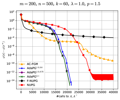
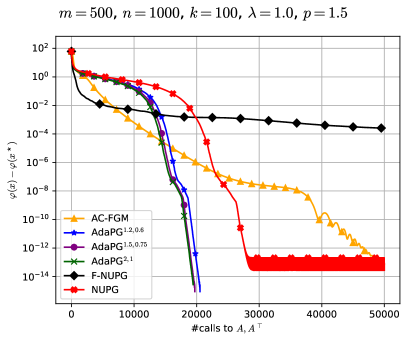
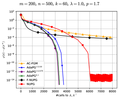
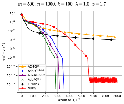
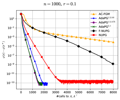
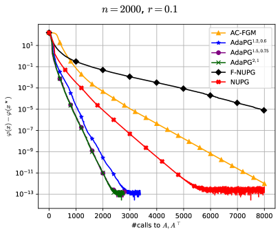
In this experiment we consider a variant of Lasso in which the squared $2$-norm is replaced with a $p$-norm raised to some power $p\in(1,2)$:

$$\min_{x\in{}^{n}}\tfrac{1}{p}\|Ax-b\|_{p}^{p}+\lambda\|x\|_{1},$$ (37)

for $A\in[-1,1]^{m\times n}$, $b\in{}^{m}$ with $n>m$ and $\lambda>0$. The first term in (37) is differentiable with globally Hölder continuous gradient with order $\nu=p-1$. The proximal mapping of the second term is the shrinkage operation which is computable in closed form. To assess the performance of the different algorithms we generate random instances of the problem using a $p$-norm version of the procedure provided in [28]. In Figure 1 we depict convergence plots for the different methods applied to random instances with varying dimensions of $A\in{}^{m\times n}$, powers $p\in(1,2)$ and number of nonzero entries $k$ of the solution $x^{\star}$. It can be seen that adaPG${}^{\pi,\frac{\pi}{2}}$ performs consistently better than Nesterov’s universal primal gradient [27] method NUPG with $\varepsilon=1e^{-12}$ in terms of evaluations of forward and backward passes (calls to $A,A^{\top}$). In this experiment adaPG${}^{\pi,\frac{\pi}{2}}$ also performs consistently better than the accelerated algorithms AC-FGM and F-NUPG.

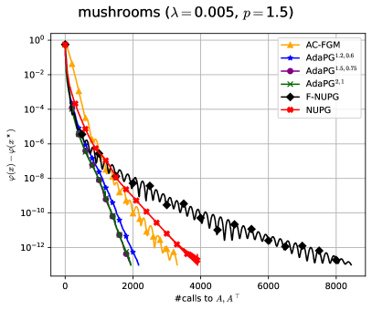
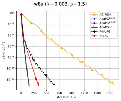
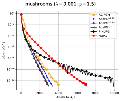
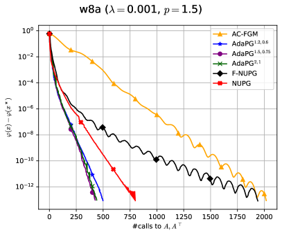
4.2 Hölder-smooth SVMs with $\ell_{1}$-regularization

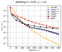
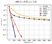
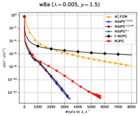
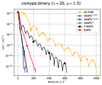
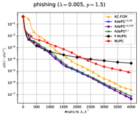
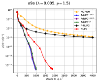
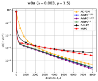
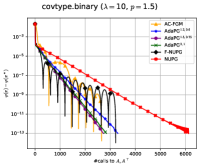
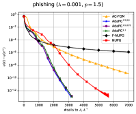
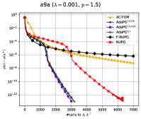
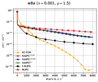
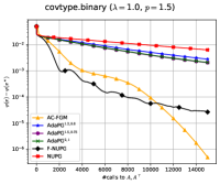
In this subsection we assess the performance of the different algorithms on the task of classification using a $p$-norm version of the SVM model. For that purpose we consider a subset of the LibSVM binary classification benchmark that consists of a collection of datasets with varying number $m$ of examples $a_{i}$, feature dimensions $n$ and sparsity. Let $(a_{j},b_{j})_{j=1}^{m}$ with $b_{j}\in\{-1,1\}$ and $a_{j}\in{}^{n}$ denote the collection of training examples. Then we consider the minimization problem

$$\min_{x\in{}^{n}}\frac{1}{m}\sum_{j=1}^{m}\tfrac{1}{p}\max\{0,1-b_{j}\langle a_{j},x\rangle\}^{p}+\lambda\|x\|_{1}.$$ (38)

for $p\in(1,2)$. The loss function is globally Hölder smooth with order $\nu=p-1$ while the proximal mapping of the second term can be solved in closed form. The results are depicted in Figure 2.

4.3 Logistic regression with $p$-norm regularization

In this subsection we consider classification with the logistic loss and a smooth $p$-norm regularizer, for some $p\in(1,2)$. The problem can be cast in convex composite minimization form as follows

$$\min_{x\in{}^{n}}\frac{1}{m}\sum_{j=1}^{m}\ln(1-\exp(b_{j}\langle a_{j},x\rangle))+\lambda\tfrac{1}{p}\|x\|_{p}^{p}.$$ (39)

Unlike the previous classification model this yields a smooth optimization problem. Hence we perform gradient steps with respect to $\varphi$ and choose the nonsmooth term $g\equiv 0$. The results are depicted in Figure 3.

Figure 3: $p$-norm regularized logistic regression. In the present cases adaPG${}^{\pi,\frac{\pi}{2}}$ performs better than the baseline algorithms.

4.4 Mixture $p$-norm regression

In this final experiment we consider the following mixture model:

$$\min_{x\in\mathbb{B}_{2}(r)}\sum_{j=1}^{J}\|A^{j}x-b^{j}\|_{p_{j}}^{p_{j}},$$ (40)

where $\mathbb{B}_{2}(r)$ is the $2$-norm ball with radius $r$ and $p_{j}\in(1,2]$. Since the $p_{j}$ are not identical the smooth part in Equation 40 is merely locally Hölder smooth. The nonsmooth part $g$ is the indicator function of the set $\mathbb{B}_{2}(r)$. In Figure 4 we compare the performance for $J=6$ with $p=(1.8,1.7,1.6,1.5,1.5,1.5)$ and two different values of $n$ where the entries of $A^{j}\in[-1,1]^{m_{j}\times n}$ and $b^{j}\in[-1,1]^{m_{j}}$ are uniformly distributed between $[-1,1]$ with $m=(400,300,400,100,100,300)$.

Figure 4: Mixture $p$-norm regression with ball constraint. It can be seen that adaPG${}^{\pi,\frac{\pi}{2}}$ performs best on this comparison. In contrast to the previous experiments, the problem involves a heterogeneous sum whose summands exhibit varying orders of Hölder differentiability.

5 Conclusions

In this paper we showed that adaptive proximal gradient methods are universal, in the sense that they converge under mere local Hölder gradient continuity of any order. This is achieved through a unified analysis of adaPG${}^{\pi,\frac{\pi}{2}}$ that encapsulates existing methods for different values of the parameter $\pi\in[1,2]$. Sequential convergence along with an $O(\nicefrac{{1}}{{K^{\nu}}})$ rate for the cost is established. Remarkably, the analysis and implementation of the algorithm does not require a priori knowledge of the order $\nu\in(0,1]$ of Hölder continuity. In other words, adaPG${}^{\pi,\frac{\pi}{2}}$ and its analysis automatically adapts to the best possible $\nu$.

The validity of some of the auxiliary results for $\nu=0$ is an encouraging indication that the algorithm could potentially cope with plain real valuedness of $f$, waiving differentiability assumptions. Whether this is really the case remains an interesting open question.

Moreover, our experiments demonstrate that adaPG${}^{\pi,\frac{\pi}{2}}$ consistently outperforms NUPG on a diverse collection of challening convex optimization problems with both locally and globally Hölder smooth costs. In many cases we observe that adaPG${}^{\pi,\frac{\pi}{2}}$ performs better than the accelerated algorithms F-NUPG and AC-FGM. We conjecture that adaPG${}^{\pi,\frac{\pi}{2}}$ exploits a hidden Hölder growth that accelerated algorithms cannot take advantage from (as is known for the classical Euclidean case under metric subregularity). In future work we aim to extend our analysis to nonconvex and stochastic settings.

Appendix

A Proofs of Section 2.1

 

Proof of Section 2.1.

The proof of assertion 1 follows by applying the Cauchy-Schwarz inequality. For assertion 2 when $\nu>0$ we refer the reader to [36, Lem. 1]; although the reference assumes global Hölder continuity, the arguments therein only use Hölder continuity of ${\nabla}f$ on the segment $[x,y]$. For the case $\nu=0$, for any $x,y\in E$ and ${\nabla}h(x)\in\partial h(x)$, ${\nabla}h(y)\in\partial h(y)$, we have

$$h(y)\leq{} h(x)+\langle{}{\nabla}h(y){},{}y-x{}\rangle$$

$$={} h(x)+\langle{}{\nabla}h(x){},{}y-x{}\rangle+\langle{}{\nabla}h(y)-{\nabla}h(x){},{}y-x{}\rangle$$

$$\leq{} h(x)+\langle{}{\nabla}h(x){},{}y-x{}\rangle+\|{\nabla}h(y)-{\nabla}h(x)\|\|y-x\|$$

$$\leq{} h(x)+\langle{}{\nabla}h(x){},{}y-x{}\rangle+{L_{{E},0}}\|y-x\|,$$

where the first inequality follows from convexity of $h$.

We now turn to the last two claims, and thus restrict to the case $\nu>0$. We will only show assertion 4, as 3 in turn follows by exchanging the roles of $x$ and $y$ and summing the corresponding inequalities. The proof follows along the lines of [2, Thm. 5.8(iii)] and is included for completeness to highlight the need of the enlarged set $\overline{E}$. We henceforth fix $x,y\in E\subseteq\overline{E}$. Since ${\nabla}f$ is $\nu$-Hölder continuous in $\overline{E}$ with modulus $L_{{\overline{E}},\nu}$, it follows from assertion 2 that

$$f(z)\leq f(y)+\langle{}{\nabla}f(y){},{}z-y{}\rangle+\tfrac{L_{{\overline{E}},\nu}}{1+\nu}\|z-y\|^{1+\nu}\quad\forall z\in\overline{E}.$$ (41)

Let $l_{x}(y)\coloneqq f(y)-f(x)-\langle{}{\nabla}f(x){},{}y-x{}\rangle$, and note that $l_{x}$ is a convex function with ${\nabla}l_{x}(y)={\nabla}f(y)-{\nabla}f(x)$. For any $z\in\overline{E}$, we have

$$l_{x}(z)={} f(z)-f(x)-\langle{}{\nabla}f(x){},{}z-x{}\rangle$$

$$\mathrel{{}\mathop{\leq}\limits^{\vphantom{\text{\scriptsize\clap{\begin{tabular}[b]{c}\eqref{eq:holder_ineq}\end{tabular}}}}\smash{\raisebox{1.5pt}{\text{\scriptsize\clap{\begin{tabular}[b]{c}\eqref{eq:holder_ineq}\end{tabular}}}}}}}{} f(y)+\langle{}{\nabla}f(y){},{}z-y{}\rangle+\tfrac{L_{{\overline{E}},\nu}}{1+\nu}\|z-y\|^{1+\nu}-f(x)-\langle{}{\nabla}f(x){},{}z-x{}\rangle$$

$$={} f(y)-f(x)-\langle{}{\nabla}f(x){},{}y-x{}\rangle+\langle{}{\nabla}f(y)-{\nabla}f(x){},{}z-y{}\rangle+\tfrac{L_{{\overline{E}},\nu}}{1+\nu}\|z-y\|^{1+\nu}$$

$$={} l_{x}(y)+\langle{}{\nabla}l_{x}(y){},{}z-y{}\rangle+\tfrac{L_{{\overline{E}},\nu}}{1+\nu}\|z-y\|^{1+\nu}.$$

Noticing that ${\nabla}l_{x}(x)=0$, it follows from convexity that $x$ is a global minimizer of $l_{x}$, hence that $\min l_{x}=l_{x}(x)=0$. Let us denote $v\coloneqq\frac{1}{\|{\nabla}l_{x}(y)\|}{\nabla}l_{x}(y)$ and define $z=y-\|{\nabla}l_{x}(y)\|^{1/\nu}L_{{\overline{E}},\nu}^{-1/\nu}v$. Note that

$$\|z-y\|=\Bigl{(}\tfrac{\|{\nabla}l_{x}(y)\|}{L_{{\overline{E}},\nu}}\Bigr{)}^{\frac{1}{\nu}}=\Bigl{(}\tfrac{\|{\nabla}f(y)-{\nabla}f(x)\|}{L_{{\overline{E}},\nu}}\Bigr{)}^{\frac{1}{\nu}}\leq\|y-x\|,$$

and in particular $z\in E+\operatorname{\overline{B}}(y;\|y-x\|)\subseteq\overline{E}$. From the previous inequality we get

$$0=\min l_{x}=l_{x}(x)\leq{} l_{x}\bigl{(}y-\|{\nabla}l_{x}(y)\|^{1/\nu}{L_{{\overline{E}},\nu}^{-1/\nu}}v\bigr{)}.$$

$$\mathrel{{}\mathop{\leq}\limits^{\vphantom{\text{\scriptsize\clap{\begin{tabular}[b]{c}\eqref{eq:holder_ineq}\end{tabular}}}}\smash{\raisebox{1.5pt}{\text{\scriptsize\clap{\begin{tabular}[b]{c}\eqref{eq:holder_ineq}\end{tabular}}}}}}}{} l_{x}(y)-\|{\nabla}l_{x}(y)\|^{1/\nu}L_{{\overline{E}},\nu}^{-1/\nu}\langle{}{\nabla}l_{x}(y){},{}v{}\rangle+\tfrac{L_{{\overline{E}},\nu}}{1+\nu}\tfrac{1}{L_{{\overline{E}},\nu}^{1+1/\nu}}\|{\nabla}l_{x}(y)\|^{1+\frac{1}{\nu}}$$

$$={} f(y)-f(x)-\langle{}{\nabla}f(x){},{}y-x{}\rangle-\tfrac{\nu}{\nu+1}\tfrac{1}{L_{{\overline{E}},\nu}^{1/\nu}}\|{\nabla}f(x)-{\nabla}f(y)\|^{1+1/\nu},$$

as claimed. ∎

 

 

Proof of Section 2.1.

Expanding the squares yields

$$\|H_{k}(x^{k})-H_{k}(x^{k-1})\|^{2}={} \|x^{k}-x^{k-1}\|^{2}+\gamma_{k}^{2}\|{\nabla}f(x^{k})-{\nabla}f(x^{k-1})\|^{2}+2\gamma_{k}\langle{}x^{k}-x^{k-1}{},{}{\nabla}f(x^{k})-{\nabla}f(x^{k-1}){}\rangle$$

$$={} \|x^{k}-x^{k-1}\|^{2}+\gamma_{k}^{2}L_{{k},\nu}^{2}\|x^{k}-x^{k-1}\|^{2\nu}+2\gamma_{k}\ell_{{k},\nu}\|x^{k}-x^{k-1}\|^{1+\nu}.$$

From the identity $\gamma_{k}=\lambda_{{k},\nu}\|x^{k}-x^{k-1}\|^{1-\nu}>0$, the claimed expression follows. ∎

 

B Proofs of Section 3.1

 

Proof of Section 3.1.

Recall the subgradient characterization

$$\widetilde{{\nabla}}g(x^{k+1})\coloneqq\tfrac{x^{k}-x^{k+1}}{\gamma_{k+1}}-{\nabla}f(x^{k})\in\partial g(x^{k+1}).$$ (42)

By monotonicity of $\partial g$,

$$\tfrac{1}{\gamma_{k+1}^{2}}\|x^{k}-x^{k+1}\|^{2}\leq{} \bigl{\|}\tfrac{x^{k}-x^{k+1}}{\gamma_{k+1}}+\widetilde{{\nabla}}g(x^{k})-\widetilde{{\nabla}}g(x^{k+1})\bigr{\|}^{2}-\bigl{\|}\widetilde{{\nabla}}g(x^{k})-\widetilde{{\nabla}}g(x^{k+1})\bigr{\|}^{2}$$

$$={} \bigl{\|}\tfrac{x^{k-1}-x^{k}}{\gamma_{k}}+{\nabla}f(x^{k})-{\nabla}f(x^{k-1})\bigr{\|}^{2}-\bigl{\|}\tfrac{x^{k-1}-x^{k}}{\gamma_{k}}+\tfrac{x^{k+1}-x^{k}}{\gamma_{k+1}}+{\nabla}f(x^{k})-{\nabla}f(x^{k-1})\bigr{\|}^{2}$$

$$={} \bigl{\|}\tfrac{x^{k-1}-x^{k}}{\gamma_{k}}\bigr{\|}^{2}+\bigl{\|}{\nabla}f(x^{k})-{\nabla}f(x^{k-1})\bigr{\|}^{2}$$

$$+\tfrac{2}{\gamma_{k}\gamma_{k+1}}\langle{}x^{k}-x^{k}{},{}x^{k-1}-x^{k}{}\rangle+\tfrac{2}{\gamma_{k}}\langle{}x^{k-1}-x^{k}{},{}{\nabla}f(x^{k})-{\nabla}f(x^{k-1}){}\rangle$$

$$-\bigl{\|}\tfrac{x^{k-1}-x^{k}}{\gamma_{k}}\bigr{\|}^{2}-\bigl{\|}\tfrac{x^{k+1}-x^{k}}{\gamma_{k+1}}\bigr{\|}^{2}-\bigl{\|}{\nabla}f(x^{k})-{\nabla}f(x^{k-1})\bigr{\|}^{2}$$

$$-\tfrac{2}{\gamma_{k}\gamma_{k+1}}\langle{}x^{k-1}-x^{k}{},{}x^{k+1}-x^{k}{}\rangle-2\langle{}\tfrac{x^{k-1}-x^{k}}{\gamma_{k}}+\tfrac{x^{k+1}-x^{k}}{\gamma_{k+1}}{},{}{\nabla}f(x^{k})-{\nabla}f(x^{k-1}){}\rangle$$

$$={} \tfrac{2}{\gamma_{k}\gamma_{k+1}}\langle{}x^{k}-x^{k+1}{},{}x^{k-1}-x^{k}{}\rangle+2\langle{}\tfrac{x^{k}-x^{k+1}}{\gamma_{k+1}}{},{}{\nabla}f(x^{k})-{\nabla}f(x^{k-1}){}\rangle-\bigl{\|}\tfrac{x^{k+1}-x^{k}}{\gamma_{k+1}}\bigr{\|}^{2}$$

$$={} \tfrac{2}{\gamma_{k}\gamma_{k+1}}\langle{}x^{k}-x^{k+1}{},{}H_{k}(x^{k-1})-H_{k}(x^{k}){}\rangle-\tfrac{1}{\gamma_{k+1}^{2}}\bigl{\|}x^{k+1}-x^{k}\bigr{\|}^{2}.$$

After moving the norm on the right-hand side and multiplying by $\frac{\gamma_{k}\gamma_{k+1}}{2}$ the claimed first inequality is obtained. The second one then follows by an application of the Cauchy-Schwarz inequality. ∎

 

 

Proof of Section 3.1.

From the convexity inequality for $g$ at $x^{k+1}$ with subgradient $\widetilde{{\nabla}}g(x^{k+1})$ as in (42), we have that for any $x\in\operatorname{dom}g$

$$0\leq{} g(x)-g(x^{k+1})+\langle{}{\nabla}f(x^{k}){},{}x-x^{k+1}{}\rangle-\tfrac{1}{\gamma_{k+1}}\langle{}x^{k}-x^{k+1}{},{}x-x^{k+1}{}\rangle$$

$$={} g(x)-g(x^{k+1})+\langle{}{\nabla}f(x^{k}){},{}x-x^{k+1}{}\rangle+\tfrac{1}{2\gamma_{k+1}}{\mathopen{}\left(\|x^{k}-x\|^{2}-\|x^{k+1}-x\|^{2}-\|x^{k}-x^{k+1}\|^{2}\right)\mathclose{}}.$$ (43)

On the other hand, using $\widetilde{{\nabla}}g(x^{k})\in\partial g(x^{k})$ yields that

$$0\leq g(x^{k+1})-g(x^{k})+\langle{}{\nabla}f(x^{k-1}){},{}x^{k+1}-x^{k}{}\rangle-\tfrac{1}{\gamma_{k}}\langle{}x^{k-1}-x^{k}{},{}x^{k+1}-x^{k}{}\rangle.$$ (44)

We now rewrite the inner product in (43) is a way that allows us to exploit the above inequality:

$$\langle{}{\nabla}f(x^{k}){},{}x-x^{k+1}{}\rangle={} \langle{}{\nabla}f(x^{k}){},{}x-x^{k}{}\rangle+\langle{}{\nabla}f(x^{k}){},{}x^{k}-x^{k+1}{}\rangle$$

$$\leq{} f(x)-f(x^{k})+\langle{}{\nabla}f(x^{k}){},{}x^{k}-x^{k+1}{}\rangle.$$

The last inner product can be controlled using (44):

$$\langle{}{\nabla}f(x^{k}){},{}x^{k}-x^{k+1}{}\rangle={} \langle{}{\nabla}f(x^{k})-{\nabla}f(x^{k-1}){},{}x^{k}-x^{k+1}{}\rangle+\langle{}{\nabla}f(x^{k-1}){},{}x^{k}-x^{k+1}{}\rangle$$

$$\leq{} \langle{}{\nabla}f(x^{k})-{\nabla}f(x^{k-1}){},{}x^{k}-x^{k+1}{}\rangle+g(x^{k+1})-g(x^{k})-\tfrac{1}{\gamma_{k}}\langle{}x^{k-1}-x^{k}{},{}x^{k+1}-x^{k}{}\rangle$$

$$={} g(x^{k+1})-g(x^{k})+\tfrac{1}{\gamma_{k}}\langle{}H_{k}(x^{k-1})-H_{k}(x^{k}){},{}x^{k}-x^{k+1}{}\rangle$$

$$\text{\footnotesize(\lx@cref{creftypeplural~refnum}{thm:FNE} and~\lx@cref{refnum}{thm:Hk})}\quad\leq{} g(x^{k+1})-g(x^{k})+\tfrac{\rho_{k+1}}{\gamma_{k}}M_{k}\|x^{k}-x^{k-1}\|^{2}.$$

Combine this with the prior inequality and (43) to obtain

$$0\leq\gamma_{k+1}(\varphi(x)-\varphi(x^{k}))+\rho_{k+1}^{2}M_{k}\|x^{k}-x^{k-1}\|^{2}+\tfrac{1}{2}{\mathopen{}\left(\|x^{k}-x\|^{2}-\|x^{k+1}-x\|^{2}-\|x^{k}-x^{k+1}\|^{2}\right)\mathclose{}}.$$

Finally, recalling the definition of $\widetilde{{\nabla}}g(x^{k})$ as in (42) we have

$${\nabla}f(x^{k})+\widetilde{{\nabla}}g(x^{k})=\tfrac{1}{\gamma_{k}}\bigl{(}H_{k}(x^{k-1})-H_{k}(x^{k})\bigr{)}=\tfrac{x^{k-1}-x^{k}}{\gamma_{k}}+{\nabla}f(x^{k})-{\nabla}f(x^{k-1})\in\partial\varphi(x^{k}).$$

Therefore, for any $\vartheta_{k+1}\geq 0$

$$0\leq{} \gamma_{k+1}\vartheta_{k+1}{\mathopen{}\left(\varphi(x^{k-1})-\varphi(x^{k})-\tfrac{1}{\gamma_{k}}\langle{}H_{k}(x^{k-1})-H_{k}(x^{k}){},{}x^{k-1}-x^{k}{}\rangle\right)\mathclose{}}$$

$$={} \gamma_{k+1}\vartheta_{k+1}{\mathopen{}\left(\varphi(x^{k-1})-\varphi(x^{k})-\tfrac{1-\gamma_{k}L_{{k},\nu}}{\gamma_{k}}\|x^{k-1}-x^{k}\|^{2}\right)\mathclose{}}.$$

Combining the last two inequalities and letting $P_{k}(x)\coloneqq\varphi(x^{k})-\varphi(x)$ yields

$${}\tfrac{1}{2}\|x^{k+1}-x\|^{2}+\gamma_{k+1}(1+\vartheta_{k+1})P_{k}(x)+\tfrac{1}{2}\|x^{k}-x^{k+1}\|^{2}$$

$$\leq{} \tfrac{1}{2}\|x^{k}-x\|^{2}+\gamma_{k+1}\vartheta_{k+1}P_{k-1}(x)-\rho_{k+1}{\mathopen{}\left(\vartheta_{k+1}(1-\gamma_{k}L_{{k},\nu})-\rho_{k+1}M_{k}\right)\mathclose{}}\|x^{k-1}-x^{k}\|^{2}$$

Letting $\vartheta_{k}=\pi\rho_{k}$ for all $k$, and setting $x=x^{\star}\in\operatorname*{arg\,min}\varphi$ establishes the claimed inequality. ∎

 

 

Proof of Section 3.1.

• 1) The update rule for $\gamma_{k}$ ensures that the coefficients of $\|x^{k}-x^{k-1}\|^{2}$ and $P_{k-1}$ in (20) are negative, and that therefore $(\mathcal{U}_{k}^{\pi}(x^{\star}))_{k\in\m@thbbch@rN}$ is decreasing. Since $\mathcal{U}_{k}^{\pi}(x^{\star})\geq 0$, the sequence converges to a finite (positive) value.

• 2) Boundedness follows by observing that $\frac{1}{2}\|x^{k}-x^{\star}\|^{2}\leq\mathcal{U}_{k}^{\pi}(x^{\star})\leq\mathcal{U}_{0}^{\pi}(x^{\star})$, where the last inequality owes to the previous assertion. In what follows, we let $L_{{\Omega},\nu}<\infty$ be a $\nu$-Hölder modulus for ${\nabla}f$ on a convex and compact set $\Omega$ that contains all the iterates $x^{k}$. In particular, $\ell_{{k},\nu}\leq L_{{k},\nu}\leq L_{{\Omega},\nu}$ holds for every $k$. Suppose that $x_{\infty}$ and $x_{\infty}^{\prime}$ are two optimal limit points, and observe that

  $$\mathcal{U}_{k}^{\pi}(x_{\infty})-\mathcal{U}_{k}^{\pi}(x_{\infty}^{\prime})=\tfrac{1}{2}\|x_{\infty}\|^{2}+\tfrac{1}{2}\|x_{\infty}^{\prime}\|^{2}+\langle{}x^{k}{},{}x_{\infty}^{\prime}-x_{\infty}{}\rangle.$$

  Since both $(\mathcal{U}_{k}^{\pi}(x_{\infty}))_{k\in\m@thbbch@rN}$ and $(\mathcal{U}_{k}^{\pi}(x_{\infty}^{\prime}))_{k\in\m@thbbch@rN}$ are convergent, by taking the limit along the subsequences converging to $x_{\infty}$ and $x_{\infty}^{\prime}$ we obtain $\langle{}x_{\infty}{},{}x_{\infty}^{\prime}-x_{\infty}{}\rangle=\langle{}x_{\infty}^{\prime}{},{}x_{\infty}^{\prime}-x_{\infty}{}\rangle$, which after rearranging yields $\|x_{\infty}-x_{\infty}^{\prime}\|^{2}=0$.

• 3) Since $\gamma_{k}(1+\pi\rho_{k}-\pi\rho_{k+1}^{2})\geq 0$ because of the update rule of $\gamma_{k+1}$, and with $P_{k}^{\rm min}\coloneqq\min_{i\leq k}P_{i}$ denoting the best-so-far cost at iteration $k$, a telescoping argument on (20) yields that

  $$P_{K}^{\rm min}\sum_{k=1}^{K}\gamma_{k}(1+\pi\rho_{k}-\pi\rho_{k+1}^{2})\leq{} \sum_{k=1}^{K}\gamma_{k}(1+\pi\rho_{k}-\pi\rho_{k+1}^{2})P_{k-1}$$

  $$\leq{} \mathcal{U}_{1}^{\pi}(x^{\star})-\mathcal{U}_{K+1}^{\pi}(x^{\star})\leq\mathcal{U}_{1}^{\pi}(x^{\star})-\gamma_{k+1}(1+\pi\rho_{K+1})P_{K}^{\rm min},$$ (45)

  hence that

  $$P_{K}^{\rm min}\leq{} \frac{\mathcal{U}_{1}^{\pi}(x^{\star})}{\sum_{k=1}^{K+1}\gamma_{k}(1+\pi\rho_{k}-\pi\rho_{k+1}^{2})+\gamma_{k+1}(1+\pi\rho_{K+1})}$$

  $$={} \frac{\mathcal{U}_{1}^{\pi}(x^{\star})}{\sum_{k=1}^{K}(\gamma_{k}+\pi\gamma_{k}\rho_{k}-\pi\gamma_{k+1}\rho_{k+1})+\gamma_{k+1}+\pi\gamma_{k+1}\rho_{K+1}}=\frac{\mathcal{U}_{1}^{\pi}(x^{\star})}{\pi\gamma_{1}\rho_{1}+\sum_{k=1}^{K+1}\gamma_{k}}.$$

  This completes the proof. ∎

 

Appendix C Implementation details of AC-FGM

In this section we describe the specific implementation of the auto-conditioned fast gradient method (AC-FGM) [22], which in our notation reads

$$z^{k+1}={} \operatorname{prox}_{\gamma_{k+1}g}(y^{k}-\gamma_{k+1}{\nabla}f(x^{k}))$$

$$y^{k+1}={} (1-\beta_{k+1})y^{k}+\beta_{k+1}z^{k+1}$$

$$x^{k+1}={} (z^{k+1}+\tau_{k+1}x^{k})/(1+\tau_{k+1}).$$

Regarding the positive sequences $(\gamma_{k})_{k\in\m@thbbch@rN},(\beta_{k})_{k\in\m@thbbch@rN},(\tau_{k})_{k\in\m@thbbch@rN}$, we use the update rule described in [22, Cor. 3] and as such in Corollary 2 of the same paper. We choose $\beta_{k}=\beta=\tfrac{1-\sqrt{3}}{2}$ for all $k\in\m@thbbch@rN$, ensure that $\gamma_{1}\in[\tfrac{\beta}{4(1-\beta)c_{1}},\tfrac{1}{3c_{1}}]$ and set $\gamma_{2}=\tfrac{\beta}{2c_{1}}$ and $\gamma_{k+1}=\min\{\tfrac{\tau_{k-1}+1}{\tau_{k}}\gamma_{k},\tfrac{\beta\tau_{k}}{4c_{k}}\}$ for all $k\geq 2$. Finally, $\tau_{1}=0$, $\tau_{2}=2$ and $\tau_{k+1}=\tau_{k}+\tfrac{\alpha}{2}+\tfrac{2(1-\alpha)\gamma_{k}c_{k}}{\beta\tau_{k}}$, for $k\geq 2$ and some $\alpha\in[0,1]$. We chose $\alpha=0$, since this configuration consistently outperfomed the others in our experiments. The sequence $(c_{k})_{k\in\m@thbbch@rN}$ is the so-called local Lipschitz estimate and is defined as in [22, Eq. (3.9)]:

$${c_{k}={\mathopen{}\left\{\begin{array}[]{l @{\hspace{\ifcasescolsep}} >{\text{if~}}l }\tfrac{\sqrt{\|x^{1}-x^{0}\|^{2}\|{\nabla}f(x^{1})-{\nabla}f(x^{0})\|^{2}+(\epsilon/4)^{2}}-\epsilon/4}{\|x^{1}-x^{0}\|^{2}}\hfil\hskip 10.00002pt&\leavevmode\nobreak\ }k=1,\\[3.0pt] \tfrac{\sqrt{\|{\nabla}f(x^{k})-{\nabla}f(x^{k-1})\|^{2}}-\epsilon/4}{2[f(x^{k-1})-f(x^{k})-\langle{}{\nabla}f(x^{k}){},{}x^{k-1}-x^{k}{}\rangle]+\epsilon/\tau_{k+1}}\hfil\hskip 10.00002pt&\lx@intercol\text{otherwise.}\hfil\lx@intercol\end{array}\right.\mathclose{}}$$

where $\epsilon$ is the predefined desired accuracy of the algorithm.

References

- [1] Heinz H. Bauschke and Patrick L. Combettes. Convex analysis and monotone operator theory in Hilbert spaces. CMS Books in Mathematics. Springer, 2017.
- [2] Amir Beck. First-order methods in optimization. SIAM, Philadelphia, PA, 2017.
- [3] Jacek Bochnak, Michel Coste, and Marie-Françoise Roy. Real algebraic geometry. Springer-Verlag Berlin Heidelberg, 1998.
- [4] Jérôme Bolte, Lilian Glaudin, Edouard Pauwels, and Mathieu Serrurier. The backtrack Hölder gradient method with application to min-max and min-min problems. Open Journal of Mathematical Optimization, 4:1–17, 2023.
- [5] Kristian Bredies. A forward–backward splitting algorithm for the minimization of non-smooth convex functionals in Banach space. Inverse Problems, 25(1):015005, 2008.
- [6] Coralia Cartis, Nicholas IM Gould, and Philippe L Toint. Adaptive cubic regularisation methods for unconstrained optimization. part i: motivation, convergence and numerical results. Mathematical Programming, 127(2):245–295, 2011.
- [7] Rick Chartrand and Wotao Yin. Iteratively reweighted algorithms for compressive sensing. In 2008 IEEE international conference on acoustics, speech and signal processing, pages 3869–3872. IEEE, 2008.
- [8] Aaron Defazio, Baoyu Zhou, and Lin Xiao. Grad-GradaGrad? A non-monotone adaptive stochastic gradient method. arXiv:2206.06900, 2022.
- [9] Olivier Devolder, François Glineur, and Yurii Nesterov. First-order methods of smooth convex optimization with inexact oracle. Mathematical Programming, 146:37–75, 2014.
- [10] Nikita Doikov, Konstantin Mishchenko, and Yurii Nesterov. Super-universal regularized Newton method. SIAM Journal on Optimization, 34(1):27–56, 2024.
- [11] John Duchi, Elad Hazan, and Yoram Singer. Adaptive subgradient methods for online learning and stochastic optimization. Journal of machine learning research, 12(7), 2011.
- [12] Alan B Forsythe. Robust estimation of straight line regression coefficients by minimizing pth power deviations. Technometrics, 14(1):159–166, 1972.
- [13] Saeed Ghadimi, Guanghui Lan, and Hongchao Zhang. Generalized uniformly optimal methods for nonlinear programming. Journal of Scientific Computing, 79:1854–1881, 2019.
- [14] Benjamin Grimmer. On optimal universal first-order methods for minimizing heterogeneous sums. Optimization Letters, pages 1–19, 2023.
- [15] Wei-Bo Guan and Wen Song. The forward–backward splitting method and its convergence rate for the minimization of the sum of two functions in Banach spaces. Optimization Letters, 15(5):1735–1758, 2021.
- [16] Yosra Hafiene, Jalal Fadili, and Abderrahim Elmoataz. Nonlocal -Laplacian variational problems on graphs. arXiv:1810.12817, 2018.
- [17] Dmitry Kamzolov, Pavel Dvurechensky, and Alexander V Gasnikov. Universal intermediate gradient method for convex problems with inexact oracle. Optimization Methods and Software, 36(6):1289–1316, 2021.
- [18] Puya Latafat, Andreas Themelis, and Panagiotis Patrinos. On the convergence of adaptive first order methods: Proximal gradient and alternating minimization algorithms. arXiv:2311.18431, 2023.
- [19] Puya Latafat, Andreas Themelis, Lorenzo Stella, and Panagiotis Patrinos. Adaptive proximal algorithms for convex optimization under local Lipschitz continuity of the gradient. arXiv:2301.04431, 2023.
- [20] Emanuel Laude and Panagiotis Patrinos. Anisotropic proximal gradient. arXiv:2210.15531, 2022.
- [21] Emanuel Laude and Panagiotis Patrinos. Anisotropic proximal point algorithm. arXiv:2312.09834, 2023.
- [22] Tianjiao Li and Guanghui Lan. A simple uniformly optimal method without line search for convex optimization. arXiv:2310.10082, 2023.
- [23] Xiaoyu Li and Francesco Orabona. On the convergence of stochastic gradient descent with adaptive stepsizes. In The 22nd International Conference on Artificial Intelligence and Statistics, pages 983–992. PMLR, 2019.
- [24] Javier Luque. Nonlinear proximal point algorithms. PhD thesis, Massachusetts Institute of Technology, Department of Civil Engineering, 1984.
- [25] Yura Malitsky and Konstantin Mishchenko. Adaptive gradient descent without descent. In Proceedings of the 37th International Conference on Machine Learning, volume 119, pages 6702–6712. PMLR, 13- 2020.
- [26] Yura Malitsky and Konstantin Mishchenko. Adaptive proximal gradient method for convex optimization. arXiv:2308.02261, 2023.
- [27] Yu Nesterov. Universal gradient methods for convex optimization problems. Mathematical Programming, 152(1-2):381–404, 2015.
- [28] Yurii Nesterov. Gradient methods for minimizing composite functions. Mathematical Programming, 140(1):125–161, aug 2013.
- [29] Yurii Nesterov. Implementable tensor methods in unconstrained convex optimization. Mathematical Programming, 186:157–183, 2021.
- [30] Yurii Nesterov. Inexact accelerated high-order proximal-point methods. Mathematical Programming, pages 1–26, 2021.
- [31] Yurii Nesterov, Alexander Gasnikov, Sergey Guminov, and Pavel Dvurechensky. Primal–dual accelerated gradient methods with small-dimensional relaxation oracle. Optimization Methods and Software, 36(4):773–810, 2021.
- [32] Konstantinos A Oikonomidis, Alexander Bodard, Emanuel Laude, and Panagiotis Patrinos. Power proximal point and augmented Lagrangian method. arXiv:2312.12205, 2023.
- [33] Ralph T. Rockafellar. Convex analysis. Princeton University Press, 1970.
- [34] Fedor Stonyakin, Alexander Tyurin, Alexander Gasnikov, Pavel Dvurechensky, Artem Agafonov, Darina Dvinskikh, Mohammad Alkousa, Dmitry Pasechnyuk, Sergei Artamonov, and Victorya Piskunova. Inexact model: A framework for optimization and variational inequalities. Optimization Methods and Software, 36(6):1155–1201, 2021.
- [35] Tianbao Yang and Qihang Lin. Rsg: Beating subgradient method without smoothness and strong convexity. The Journal of Machine Learning Research, 19(1):236–268, 2018.
- [36] Maryam Yashtini. On the global convergence rate of the gradient descent method for functions with Hölder continuous gradients. Optimization letters, 10:1361–1370, 2016.
- [37] Yiming Ying and Ding-Xuan Zhou. Unregularized online learning algorithms with general loss functions. Applied and Computational Harmonic Analysis, 42(2):224–244, 2017.
- [38] Alp Yurtsever, Alex Gu, and Suvrit Sra. Three operator splitting with subgradients, stochastic gradients, and adaptive learning rates. Advances in Neural Information Processing Systems, 34:19743–19756, 2021.
- [39] Alp Yurtsever, Quoc Tran Dinh, and Volkan Cevher. A universal primal-dual convex optimization framework. Advances in Neural Information Processing Systems, 28, 2015.
- [40] Danqing Zhou, Shiqian Ma, and Junfeng Yang. AdaBB: Adaptive Barzilai-Borwein method for convex optimization. arXiv:2401.08024, 2024.