Scalable Nonlinear Learning with
Adaptive Polynomial Expansions

Abstract

Can we effectively learn a nonlinear representation in time comparable to linear learning? We describe a new algorithm that explicitly and adaptively expands higher-order interaction features over base linear representations. The algorithm is designed for extreme computational efficiency, and an extensive experimental study shows that its computation/prediction tradeoff ability compares very favorably against strong baselines.

1 Introduction

When faced with large datasets, it is commonly observed that using all the data with a simpler algorithm is superior to using a small fraction of the data with a more computationally intense but possibly more effective algorithm. The question becomes: What is the most sophisticated algorithm that can be executed given a computational constraint?

At the largest scales, Naïve Bayes approaches offer a simple, easily distributed single-pass algorithm. A more computationally difficult, but commonly better-performing approach is large scale linear regression, which has been effectively parallelized in several ways on real-world large scale datasets [19, 1]. Is there a modestly more computationally difficult approach that allows us to commonly achieve superior statistical performance?

The approach developed here starts with a fast parallelized online learning algorithm for linear models, and explicitly and adaptively adds higher-order interaction features over the course of training, using the learned weights as a guide. The resulting space of polynomial functions increases the approximation power over the base linear representation at a modest increase in computational cost.

Several natural folklore baselines exist. For example, it is common to enrich feature spaces with $n$-grams or low-order interactions. These approaches are naturally computationally appealing, because these nonlinear features can be computed on-the-fly avoiding I/O bottlenecks. With I/O bottlenecked datasets, this can sometimes even be done so efficiently that the additional computational complexity is negligible, so improving over this baseline is quite challenging.

Figure 1: Computation/prediction tradeoff points using non-adaptive polynomial expansions and adaptive polynomial expansions ($\mathtt{apple}$). The markers are positioned at the coordinate-wise median of $(\mathtt{relative\ error},\mathtt{relative\ time})$ over $30$ datasets, with bars extending to $25$th and $75$th percentiles. See Section 3 for definition of relative error and relative time used here.

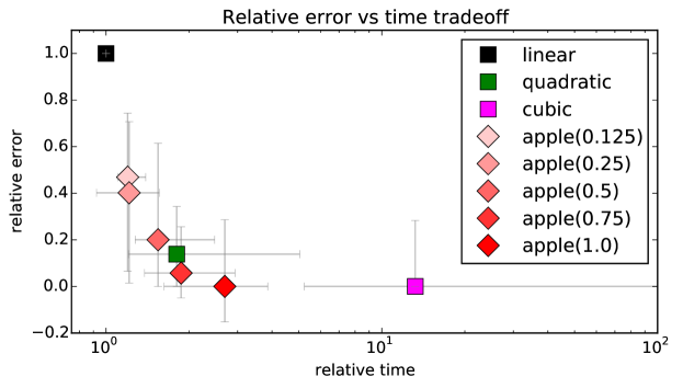
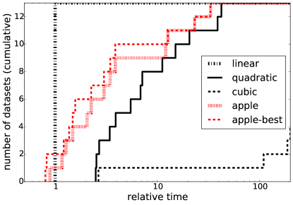
The design of our algorithm is heavily influenced by considerations for computational efficiency, as discussed further in Section 2. Several alternative designs are plausible but fail to provide adequate computation/prediction tradeoffs or even outperform the aforementioned folklore baselines. An extensive experimental study in Section 3 compares efficient implementations of these baselines with the proposed mechanism and gives strong evidence of the latter’s dominant computation/prediction tradeoff ability (see Figure 1 for an illustrative summary).

Although it is notoriously difficult to analyze nonlinear algorithms, it turns out that two aspects of this algorithm are amenable to analysis. First, we prove a regret bound showing that we can effectively compete with a growing feature set. Second, we exhibit simple problems where this algorithm is effective, and discuss a worst-case consistent variant.

Related work.

This work considers methods for enabling nonlinear learning directly in a highly-scalable learning algorithm. Starting with a fast algorithm is desirable because it more naturally allows one to improve statistical power by spending more computational resources until a computational budget is exhausted. In contrast, many existing techniques start with a (comparably) slow method (e.g., kernel SVM [28], batch PCA [17], batch least-squares regression [17]), and speed it up by sacrificing statistical power, often just to allow the algorithm to run at all on massive data sets. Similar challenges also arise in exploring the tradeoffs with boosting [8], where typical weak learners involve either exhaustive search or batch algorithms (e.g., decision tree induction [9, 13]) that present their own challenges in scaling and parallelization.

A standard alternative to explicit polynomial expansions is to employ polynomial kernels with the kernel trick [24]. While kernel methods generally have computation scaling at least quadratically with the number of training examples, a number of approximations schemes have been developed to enable a better tradeoff. The Nyström method (and related techniques) can be used to approximate the kernel matrix while permitting faster training [28]. However, these methods still suffer from the drawback that the model size after $n$ examples is typically $O(n)$. As a result, even single pass online implementations [4] typically suffer from $O(n^{2})$ training and $O(n)$ testing time complexity.

Another class of approximation schemes for kernel methods involves random embeddings into a high (but finite) dimensional Euclidean space such that the standard inner product there approximates the kernel function [21, 15, 20, 11]. Recently, such schemes have been developed for polynomial kernels [15, 20, 11] with computational scaling roughly linear in the polynomial degree. However, for many sparse, high-dimensional datasets (such as text data), the embedding of [20] creates dense, high dimensional examples, which leads to a substantial increase in computational complexity. Moreover, neither of the embeddings from [15, 20] exhibits good statistical performance unless combined with dense linear dimension reduction [11], which again results in dense vector computations. Such feature construction schemes are also typically unsupervised, while the method proposed here makes use of label information.

Learning sparse polynomial functions is primarily a computational challenge. This is because the naïve approach of combining explicit, non-adaptive polynomial expansions with sparse regression is statistically sound; the problem is its running time, which scales with $d^{\ell}$ for degree-$\ell$ polynomials in $d$ dimensions. Among methods proposed for beating this $d^{\ell}$ running time [12, 23, 14, 2, 6], all but [23] are batch algorithms (and suffer from similar drawbacks as boosting). The method of [23] uses online optimization together with an adaptive rule for creating interaction features. A variant of this is discussed in Section 2 and is used in the experimental study in Section 3 as a baseline.

2 Adaptive polynomial expansions

This section describes our new learning algorithm, $\mathtt{apple}$, which is based on stochastic gradient descent and explicit feature expansions that are adaptively defined. The specific feature expansion strategy used in $\mathtt{apple}$ is justified in some simple examples, and the use of stochastic gradient descent is backed by a new regret analysis for shifting comparators.

2.1 Algorithm description

Algorithm 1 Adaptive Polynomial Expansion ($\mathtt{apple}$)

0:  Initial features $S_{1}=\{x_{1},\ldots,x_{d}\}$, expansion sizes $(s_{k})$, epoch schedule $(\tau_{k})$, stepsizes $(\eta_{t})$.

1:  Initial weights $\boldsymbol{w}_{1}:=\boldsymbol{0}$, initial epoch $k:=1$, parent set $P_{1}:=\emptyset$.

2:  for $t=1,2,\dotsc$: do

3:     Receive stochastic gradient $\boldsymbol{g}_{t}$.

4:     Update weights:  $\boldsymbol{w}_{t+1}:=\boldsymbol{w}_{t}-\eta_{t}[\boldsymbol{g}_{t}]_{S_{k}}$, where $[\cdot]_{S_{k}}$ denotes restriction to monomials in the feature set $S_{k}$.

5:     if $t=\tau_{k}$ then

6:        Let $M_{k}\subseteq S_{k}$ be the top $s_{k}$ monomials $m(\boldsymbol{x})\in S_{k}$ such that $m(\boldsymbol{x})\notin P_{k}$, ordered from highest-to-lowest by the weight magnitude in $\boldsymbol{w}_{t+1}$.

7:        Expand feature set:  $S_{k+1}:=S_{k}\cup\{x_{i}\cdot m(\boldsymbol{x}):i\in[d],m(\boldsymbol{x})\in M_{k}\}$,  and         $P_{k+1}:=P_{k}\cup\{m(\boldsymbol{x}):m(\boldsymbol{x})\in M_{k}\}$.

8:        $k:=k+1$.

9:     end if

10:  end for

The pseudocode for $\mathtt{apple}$ is given in Algorithm 1. We regard weight vectors $\boldsymbol{w}_{t}$ and gradients $\boldsymbol{g}_{t}$ as members of a vector space with coordinate basis corresponding to monomials over the base variables $\boldsymbol{x}=(x_{1},x_{2},\dotsc,x_{d})$, up to some large but finite maximum degree.

The algorithm proceeds as stochastic gradient descent over the current feature set to update a weight vector. At specified times $\tau_{k}$, the feature set $S_{k}$ is expanded to $S_{k+1}$ by taking the top monomials in the current feature set, ordered by weight magnitude in the current weight vector, and creating interaction features between these monomials and $\boldsymbol{x}$. Care is exercised to not repeatedly pick the same monomial for creating higher order monomial by tracking a parent set $P_{k}$, the set of all monomials for which higher degree terms have been expanded. We provide more intuition for our choice of this feature growing heuristic in Section 2.3.

There are two benefits to this staged process. Computationally, the stages allow us to amortize the cost of the adding of monomials—which is implemented as an expensive dense operation—over several other (possibly sparse) operations. Statistically, using stages guarantees that the monomials added in the previous stage have an opportunity to have their corresponding parameters converge. We have found it empirically effective to set $s_{k}:=\operatorname{average}\left\|[\boldsymbol{g}_{t}]_{S_{1}}\right\|_{0}$, and to update the feature set at a constant number of equally-spaced times over the entire course of learning. In this case, the number of updates (plus one) bounds the maximum degree of any monomial in the final feature set.

2.2 Shifting comparators and a regret bound for regularized objectives

Standard regret bounds compare the cumulative loss of an online learner to the cumulative loss of a single predictor (comparator) from a fixed comparison class. Shifting regret is a more general notion of regret, where the learner is compared to a sequence of comparators $\boldsymbol{u}_{1},\boldsymbol{u}_{2},\dotsc,\boldsymbol{u}_{T}$.

Existing shifting regret bounds can be used to loosely justify the use of online gradient descent methods over expanding feature spaces [29]. These bounds are roughly of the form $\sum_{t=1}^{T}f_{t}(\boldsymbol{w}_{t})-f_{t}(\boldsymbol{u}_{t})\lesssim\sqrt{T\sum_{t<T}\left\|\boldsymbol{u}_{t}-\boldsymbol{u}_{t+1}\right\|}$, where $\boldsymbol{u}_{t}$ is allowed to use the same features available to $\boldsymbol{w}_{t}$, and $f_{t}$ is the convex cost function in step $t$. This suggests a relatively high cost for a substantial total change in the comparator, and thus in the feature space. Given a budget, one could either do a liberal expansion a small number of times, or opt for including a small number of carefully chosen monomials more frequently. We have found that the computational cost of carefully picking a small number of high quality monomials is often quite high. With computational considerations at the forefront, we will prefer a more liberal but infrequent expansion. This also effectively exposes the learning algorithm to a large number of nonlinearities quickly, allowing their parameters to jointly converge between the stages.

It is natural to ask if better guarantees are possible under some structure on the learning problem. Here, we consider the stochastic setting (rather than the harsher adversarial setting of [29]), and further assume that our objective takes the form

$$f(\boldsymbol{w}):=\mathbb{E}[\ell(\left\langle\boldsymbol{w},\boldsymbol{x}y\right\rangle)]+\lambda\|\boldsymbol{w}\|^{2}/2,$$ (1)

where the expectation is under the (unknown) data generating distribution $D$ over $(\boldsymbol{x},y)\in S\times\mathbb{R}$, and $\ell$ is some convex loss function on which suitable restrictions will be placed. Here $S$ is such that $S_{1}\subseteq S_{2}\subseteq\ldots\subseteq S$, based on the largest degree monomials we intend to expand. We assume that in round $t$, we observe a stochastic gradient of the objective $f$, which is typically done by first sampling $(\boldsymbol{x}_{t},y_{t})\sim D$ and then evaluating the gradient of the regularized objective on this sample.

This setting has some interesting structural implications over the general setting of online learning with shifting comparators. First, the fixed objective $f$ gives us a more direct way of tracking the change in comparator through $f(\boldsymbol{u}_{t})-f(\boldsymbol{u}_{t+1})$, which might often be milder than $\left\|\boldsymbol{u}_{t}-\boldsymbol{u}_{t+1}\right\|$. In particular, if $\boldsymbol{u}_{t}=\arg\min_{\boldsymbol{u}\in S_{k}}f(\boldsymbol{u})$ in epoch $k$, for a nested subspace sequence $S_{k}$, then we immediately obtain $f(\boldsymbol{u}_{t+1})\leq f(\boldsymbol{u}_{t})$. Second, the strong convexity of the regularized objective enables the possibility of faster $O(1/T)$ rates than prior work [29]. Indeed, in this setting, we obtain the following stronger result. We use the shorthand $\mathbb{E}_{t}[\cdot]$ to denote the conditional expectation at time $t$, conditioning over the data from rounds $1,\ldots,t-1$.

Theorem 1.

Let a distribution over $(\boldsymbol{x},y)$, twice differentiable convex loss $\ell$ with $\ell\geq 0$ and $\max\{\ell^{\prime},\ell^{\prime\prime}\}\leq 1$, and a regularization parameter $\lambda>0$ be given. Recall the definition (1) of the objective $f$. Let $(\boldsymbol{w}_{t},\boldsymbol{g}_{t})_{t\geq 1}$ be as specified by $\mathtt{apple}$ with step size $\eta_{t}:=1/(\lambda(t+1))$, where $\mathbb{E}_{t}([\boldsymbol{g}_{t}]_{S_{(t)}})=[\nabla f(\boldsymbol{w}_{t})]_{S_{(t)}}$ and $S_{(t)}$ is the support set corresponding to epoch $k_{t}$ at time $t$ in $\mathtt{apple}$. Then for any comparator sequence $(\boldsymbol{u}_{t})_{t=1}^{\infty}$ satisfying $\boldsymbol{u}_{t}\in S_{(t)}$, for any fixed $T\geq 1$,

$$\mathbb{E}\left(f(\boldsymbol{w}_{T+1})-\frac{\sum_{t=1}^{T}(t+2)f(\boldsymbol{u}_{t})}{\sum_{t=1}^{T}(t+2)}\right) \leq\frac{1}{T+1}\left(\frac{(X^{2}+\lambda)(X+\lambda D)^{2}}{2\lambda^{2}}\right),$$

where $X\geq\max_{t}\|\boldsymbol{x}_{t}y_{t}\|$ and $D\geq\max_{t}\max\{\|\boldsymbol{w}_{t}\|,\|\boldsymbol{u}_{t}\|\}$.

Quite remarkably, the result exhibits no dependence on the cumulative shifting of the comparators unlike existing bounds [29]. This is the first result of this sort amongst shifting bounds to the best of our knowledge, and the only one that yields $1/T$ rates of convergence even with strong convexity, something that the standard analysis fails to do. Of course, we limit ourselves to the stochastic setting for this improvement, and prove expected regret guarantees on the final predictor $\boldsymbol{w}_{T}$ as opposed to a bound on $\sum_{t=1}^{T}f(\boldsymbol{w}_{t})/T$ which is often studied even in stochastic settings.

A curious distinction is our comparator, which we believe gives us intuition for the source of our improved result. Note that standard shifting regret bounds [29] can be thought of as comparing $f(\boldsymbol{w}_{t})$ to $f(\boldsymbol{u}_{t})$, which is a harder comparison than the weighted average of $f(\boldsymbol{u}_{t})$ that we compare to—we discuss the particular non-uniform weighting in the next paragraph. Critically, averages are slower moving objects and hence the yardsticks at time $t$ and $t+1$ differ only by $O(1/t)$. This observation can be immediately combined with the known results of Zinkevich [29] to show a $O(\sqrt{T})$ cumulative regret bound against an averaged comparator sequence, without needing any strong convexity or smoothness assumptions on $f$. However, it does not immediately yield rates on the individual iterates $f(\boldsymbol{w}_{t})$ even after making these additional assumptions. Given the way our algorithm utilizes the weights to grow the support sets, such a guarantee is necessary and hence establish the result in Theorem 1.

As mentioned above, our comparator is a weighted average of $f(\boldsymbol{u}_{t})$ as opposed to the more standard uniform average. Supposing again that $f(\boldsymbol{u}_{t+1})\leq f(\boldsymbol{u}_{t})$, the weighted average comparator is a strictly harder benchmark than an unweighted average and overemphasizes the later comparator terms which are based on larger support sets. Indeed, this is a nice compromise between competing against $\boldsymbol{u}_{T}$, which is the hardest yardstick, and $\boldsymbol{u}_{1}$, which is what a standard non-shifting analysis compares to. Overall, this result demonstrates that in our setting, while there is generally a cost to be paid for shifting the comparator too much, it can still be effectively controlled in favorable cases. One problem for future work is to establish these fast $1/T$ rates also with high probability; as detailed in Appendix A (which moreover contains the proof of Theorem 1), existing techniques yield only an $O(\sqrt{T})$ bound on the deviation term.

2.3 Feature expansion heuristics

Previous work on learning sparse polynomials [23] suggests that it is possible to anticipate the utility of interaction features before even evaluating them. For instance, one of the algorithms from [23] orders monomials $m(\boldsymbol{x})$ by an estimate of $\mathbb{E}[r(\boldsymbol{x})^{2}m(\boldsymbol{x})^{2}]/\mathbb{E}[m(\boldsymbol{x})^{2}]$, where $r(\boldsymbol{x})=\mathbb{E}[y|\boldsymbol{x}]-\hat{f}(\boldsymbol{x})$ is the residual of the current predictor $\hat{f}$ (for least-squares prediction of the label $y$). Such an index is shown to be related to the potential error reduction by polynomials with $m(\boldsymbol{x})$ as a factor. We call this the SSM heuristic (after the authors of [23], though it differs from their original algorithm).

Another plausible heuristic, which we use in Algorithm 1, simply orders the monomials in $S_{k}$ by their weight magnitude in the current weight vector. We can justify this weight heuristic in the following simple example. Suppose a target function $\mathbb{E}[y|\boldsymbol{x}]$ is just a single monomial in $\boldsymbol{x}$, say, $m(\boldsymbol{x}):=\prod_{i\in M}x_{i}$ for some $M\subseteq[d]$, and that $\boldsymbol{x}$ has a product distribution over $\{0,1\}^{d}$ with $0<\mathbb{E}[x_{i}]=:p\leq 1/2$ for all $i\in[d]$. Suppose we repeatedly perform $1$-sparse regression with the current feature set $S_{k}$, and pick the top weight magnitude monomial for inclusion in the parent set $P_{k+1}$. It is easy to show that the weight on a degree $\ell$ sub-monomial of $m(\boldsymbol{x})$ in this regression is $p^{|M|-\ell}$, and the weight is strictly smaller for any term which is not a proper sub-monomial of $m(\boldsymbol{x})$. Thus we repeatedly pick the largest available sub-monomial of $m(\boldsymbol{x})$ and expand it, eventually discovering $m(\boldsymbol{x})$. After $k$ stages of the algorithm, we have at most $kd$ features in our regression here, and hence we find $m(\boldsymbol{x})$ with a total of $d|M|$ variables in our regression, as opposed to $d^{|M|}$ which typical feature selection approaches would need. This intuition can be extended more generally to scenarios where we do not necessarily do a sparse regression and beyond product distributions, but we find that even this simplest example illustrates the basic motivations underlying our choice—we want to parsimoniously expand on top of a base feature set, while still making progress towards a good polynomial for our data.

2.4 Fall-back risk-consistency

Neither the SSM heuristic nor the weight heuristic is rigorously analyzed (in any generality). Despite this, the basic algorithm $\mathtt{apple}$ can be easily modified to guarantee a form of risk consistency, regardless of which feature expansion heuristic is used. Consider the following variant of the support update rule in the algorithm $\mathtt{apple}$. Given the current feature budget $s_{k}$, we add $s_{k}-1$ monomials ordered by weight magnitudes as in Step 7. We also pick a monomial $m(\boldsymbol{x})$ of the smallest degree such that $m(\boldsymbol{x})\notin P_{k}$. Intuitively, this ensures that all degree 1 terms are in $P_{k}$ after $d$ stages, all degree 2 terms are in $P_{k}$ after $k=O(d^{2})$ stages and so on. In general, it is easily seen that $k=O(d^{\ell-1})$ ensures that all degree $\ell-1$ monomials are in $P_{k}$ and hence all degree $\ell$ monomials are in $S_{k}$. For ease of exposition, let us assume that $s_{k}$ is set to be a constant $s$ independent of $k$. Then the total number of monomials in $P_{k}$ when $k=O(d^{\ell-1})$ is $O(sd^{\ell-1})$, which means the total number of features in $S_{k}$ is $O(sd^{\ell})$.

Suppose we were interested in competing with all $\gamma$-sparse polynomials of degree $\ell$. The most direct approach would be to consider the explicit enumeration of all monomials of degree up to $\ell$, and then perform $\ell_{1}$-regularized regression [26] or a greedy variable selection method such as OMP [27] as means of enforcing sparsity. This ensures consistent estimation with $n=O(\gamma\log d^{\ell})=O(\gamma\ell\log d)$ examples. In contrast, we might need $n=O(\gamma(\ell\log d+\log s))$ examples in the worst case using this fall back rule, a minor overhead at best. However, in favorable cases, we stand to gain a lot when the heuristic succeeds in finding good monomials rapidly. Since this is really an empirical question, we will address it with our empirical evaluation.

3 Experimental study

We now describe our empirical evaluation of $\mathtt{apple}$.

3.1 Implementation, experimental setup, and performance metrics

In order to assess the effectiveness of our algorithm, it is critical to build on top of an efficient learning framework that can handle large, high-dimensional datasets. To this end, we implemented $\mathtt{apple}$ in the Vowpal Wabbit (henceforth VW) open source machine learning software. VW is a good framework for us, since it also natively supports quadratic and cubic expansions on top of the base features. These expansions are done dynamically at run-time, rather than being stored and read from disk in the expanded form for computational considerations. To deal with these dynamically enumerated features, VW uses hashing to associate features with indices, mapping each feature to a $b$-bit index, where $b$ is a parameter. The core learning algorithm is an online algorithm as assumed in $\mathtt{apple}$, but uses refinements of the basic stochastic gradient descent update (e.g., [7, 18, 16, 22]).

We implemented $\mathtt{apple}$ such that the total number of epochs was always 6 (meaning 5 rounds of adding new features). At the end of each epoch, the non-parent monomials with largest magnitude weights were marked as parents. Recall that the number of parents is modulated at $s^{\alpha}$ for some $\alpha>0$, with $s$ being the average number of non-zero features per example in the dataset so far. We will present experimental results with different choices of $\alpha$, and we found $\alpha=1$ to be a reliable default. Upon seeing an example, the features are enumerated on-the-fly by recursively expanding the marked parents, taking products with base monomials. These operations are done in a way to respect the sparsity (in terms of base features) of examples which many of our datasets exhibit.

Since the benefits of nonlinear learning over linear learning themselves are very dataset dependent, and furthermore can vary greatly for different heuristics based on the problem at hand, we found it important to experiment with a large testbed consisting of a diverse collection of medium and large-scale datasets. To this end, we compiled a collection of 30 publicly available datasets, across a number of KDDCup challenges, UCI repository and other common resources (detailed in the appendix). For all the datasets, we tuned the learning rate for each learning algorithm based on the progressive validation error (which is typically a reliable bound on test error) [3]. The number of bits in hashing was set to 18 for all algorithms, apart from cubic polynomials, where using 24 bits for hashing was found to be important for good statistical performance. For each dataset, we performed a random split with 80% of the data used for training and the remainder for testing. For all datasets, we used squared-loss to train, and $0$-$1$/squared-loss for evaluation in classification/regression problems. We also experimented with $\ell_{1}$ and $\ell_{2}$ regularization, but these did not help much. The remaining settings were left to their VW defaults.

For aggregating performance across 30 diverse datasets, it was important to use error and running time measures on a scale independent of the dataset. Let $\mathtt{\ell}$, $\mathtt{q}$ and $\mathtt{c}$ refer to the test errors of linear, quadratic and cubic baselines respectively (with $\mathtt{lin}$, $\mathtt{quad}$, and $\mathtt{cubic}$ used to denote the baseline algorithms themselves). For an algorithm $\mathtt{alg}$, we compute the relative (test) error:

$$\mathrm{rel\,err}(\mathtt{alg})=\frac{\mathrm{err}(\mathtt{alg})-\min(\mathtt{\ell},\mathtt{q},\mathtt{c})}{\max(\mathtt{\ell},\mathtt{q},\mathtt{c})-\min(\mathtt{\ell},\mathtt{q},\mathtt{c})},$$ (2)

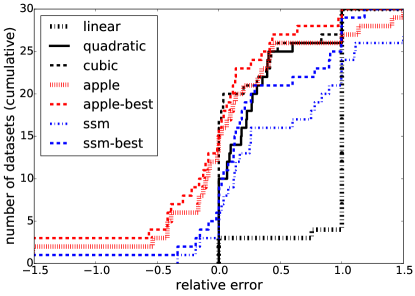
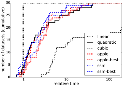
where $\min(\mathtt{\ell},\mathtt{q},\mathtt{c})$ is the smallest error among the three baselines on the dataset, and $\max(\mathtt{\ell},\mathtt{q},\mathtt{c})$ is similarly defined. We also define the relative (training) time as the ratio to running time of $\mathtt{lin}$: $\mathrm{rel\,time}(\mathtt{alg})=\mathrm{time}(\mathtt{alg})/\mathrm{time}(\mathtt{lin})$. With these definitions, the aggregated plots of relative errors and relative times for the various baselines and our methods are shown in Figure 2. For each method, the plots show a cumulative distribution function (CDF) across datasets: an entry $(a,b)$ on the left plot indicates that the relative error for $b$ datasets was at most $a$. The plots include the baselines $\mathtt{lin},\mathtt{quad},\mathtt{cubic}$, as well as a variant of $\mathtt{apple}$ (called $\mathtt{ssm}$) that replaces the weight heuristic with the SSM heuristic, as described in Section 2.3. For $\mathtt{apple}$ and $\mathtt{ssm}$, the plot shows the results with the fixed setting of $\alpha=1$, as well as the best setting chosen per dataset from $\alpha\in\{0.125,0.25,0.5,0.75,1\}$ (referred to as $\mathtt{apple}$-best and $\mathtt{ssm}$-best).

(a)	(b)

Figure 2: Dataset CDFs across all 30 datasets: (a) relative test error, (b) relative training time (log scale). $\{\mathtt{apple},\mathtt{ssm}\}$ refer to the $\alpha=1$ default; $\{\mathtt{apple},\mathtt{ssm}\}$-best picks best $\alpha$ per dataset.

3.2 Results

In this section, we present some aggregate results. Detailed results with full plots and tables are presented in the appendix. In the Figure 2(a), the relative error for all of $\mathtt{lin}$, $\mathtt{quad}$ and $\mathtt{cubic}$ is always to the right of 0 (due to the definition of $\mathrm{rel\,err}$). In this plot, a curve enclosing a larger area indicates, in some sense, that one method uniformly dominates another. Since $\mathtt{apple}$ uniformly dominates $\mathtt{ssm}$ statistically (with only slightly longer running times), we restrict the remainder of our study to comparing $\mathtt{apple}$ to the baselines $\mathtt{lin}$, $\mathtt{quad}$ and $\mathtt{cubic}$. We found that on 12 of the 30 datasets, the relative error was negative, meaning that $\mathtt{apple}$ beats all the baselines. A relative error of 0.5 indicates that we cover at least half the gap between $\min(\mathtt{\ell},\mathtt{q},\mathtt{c})$ and $\max(\mathtt{\ell},\mathtt{q},\mathtt{c})$. We find that we are below 0.5 on 27 out of 30 datasets for $\mathtt{apple}$-best, and 26 out of the 30 datasets for the setting $\alpha=1$. This is particularly striking since the error $\min(\mathtt{\ell},\mathtt{q},\mathtt{c})$ is attained by $\mathtt{cubic}$ on a majority of the datasets (17 out of 30), where the relative error of $\mathtt{cubic}$ is 0. Hence, statistically $\mathtt{apple}$ often outperforms even $\mathtt{cubic}$, while typically using a much smaller number of features. To support this claim, we include in the appendix a plot of the average number of features per example generated by each method, for all datasets. Overall, we find the statistical performance of $\mathtt{apple}$ from Figure 2 to be quite encouraging across this large collection of diverse datasets.

(a)	(b)

Figure 3: Dataset CDFs across 13 datasets where $\mathrm{time}(\mathtt{quad})\geq 2\mathrm{time}(\mathtt{lin})$: (a) relative test error, (b) relative training time (log scale).

The running time performance of $\mathtt{apple}$ is also extremely good. Figure 2(b) shows that the running time of $\mathtt{apple}$ is within a factor of 10 of $\mathtt{lin}$ for almost all datasets, which is quite impressive considering that we generate a potentially much larger number of features. The gap between $\mathtt{lin}$ and $\mathtt{apple}$ is particularly small for several large datasets, where the examples are sparse and high-dimensional. In these cases, all algorithms are typically I/O-bottlenecked, which is the same for all algorithms due to the dynamic feature expansions used. It is easily seen that the statistically efficient baseline of $\mathtt{cubic}$ is typically computationally infeasible, with the relative time often being as large as $10^{2}$ and $10^{5}$ on the biggest dataset. Overall, the statistical performance of $\mathtt{apple}$ is competitive with and often better than $\min(\mathtt{\ell},\mathtt{q},\mathtt{c})$, and offers a nice intermediate in computational complexity.

A surprise in Figure 2(b) is that $\mathtt{quad}$ appears to computationally outperform $\mathtt{apple}$ for a relatively large number of datasets, at least in aggregate. This is due to the extremely efficient implementation of $\mathtt{quad}$ in VW: on 17 of 30 datasets, the running time of $\mathtt{quad}$ is less than twice that of $\mathtt{lin}$. While we often statistically outperform $\mathtt{quad}$ on many of these smaller datasets, we are primarily interested in the larger datasets where the relative cost of nonlinear expansions (as in $\mathtt{quad}$) is high.

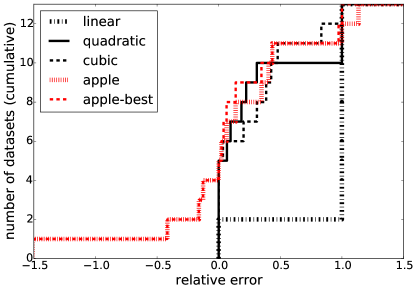
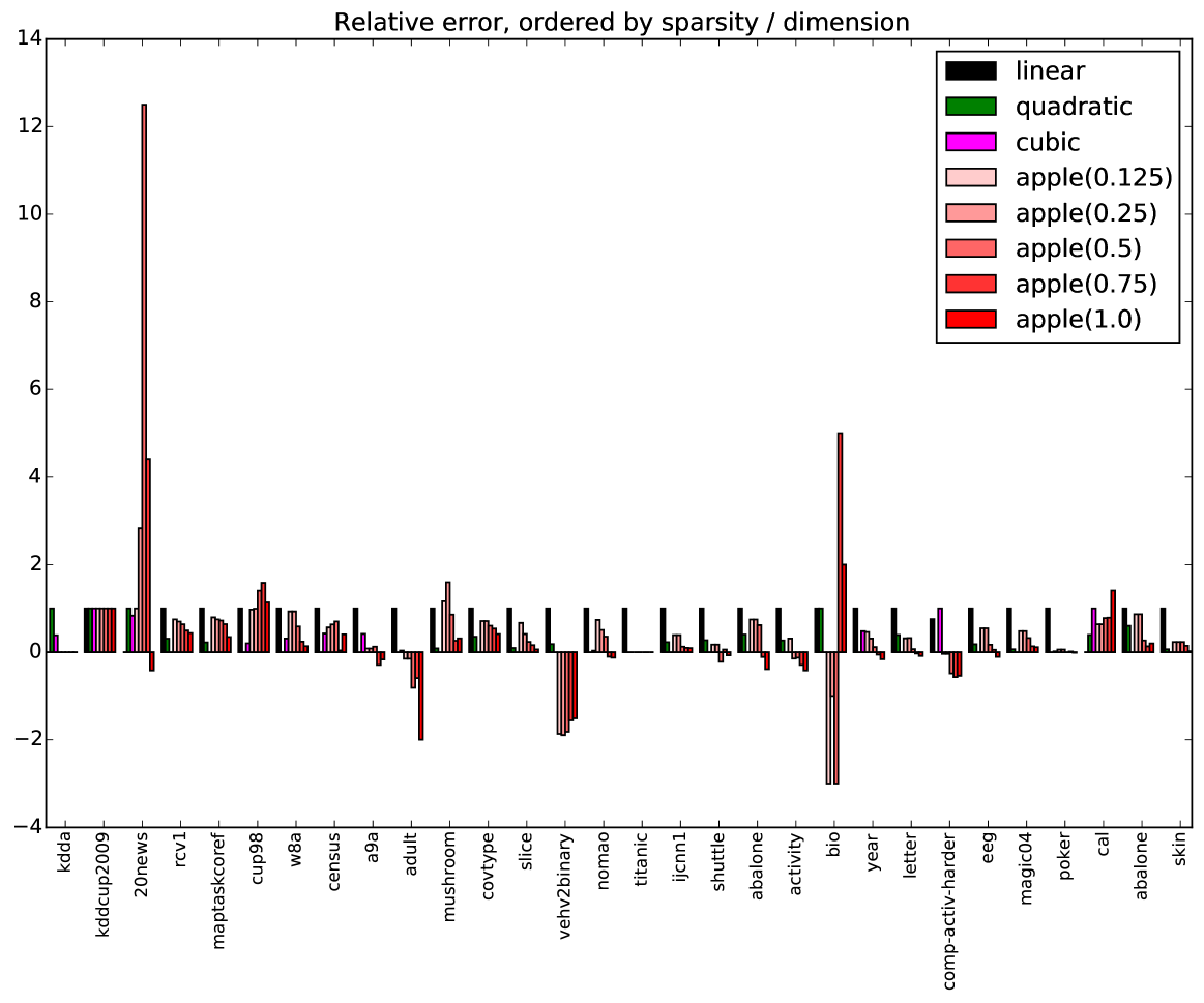
In Figure 3, we restrict attention to the 13 datasets where $\mathrm{time}(\mathtt{quad})/\mathrm{time}(\mathtt{lin})\geq 2$. On these larger datasets, our statistical performance seems to dominate all the baselines (at least in terms of the CDFs, more on individual datasets will be said later). In terms of computational time, we see that we are often much better than $\mathtt{quad}$, and $\mathtt{cubic}$ is essentially infeasible on most of these datasets. This demonstrates our key intuition that such adaptively chosen monomials are key to effective nonlinear learning in large, high-dimensional datasets.

We also experimented with picky algorithms of the sort mentioned in Section 2.2. We tried the original algorithm from [23], which tests a candidate monomial before adding it to the feature set $S_{k}$, rather than just testing candidate parent monomials for inclusion in $P_{k}$; and also a picky algorithm based on our weight heuristic. Both algorithms were extremely computationally expensive, even when implemented using VW as a base: the explicit testing for inclusion in $S_{k}$ (on a per-example basis) caused too much overhead. We ruled out other baselines such as polynomial kernels for similar computational reasons.

(a)	(b)

Figure 4: Comparison of different methods on the top 6 datasets by non-zero features per example: (a) relative test errors, (b) relative training times.

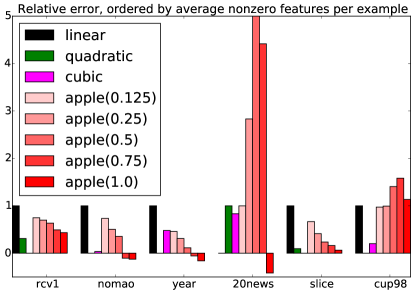
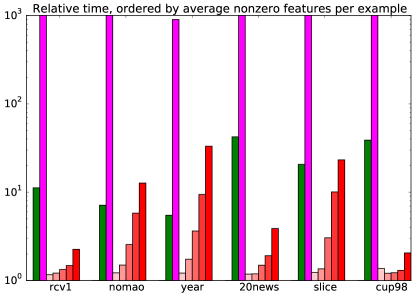
To provide more intuition, we also show individual results for the top 6 datasets with the highest average number of non-zero features per example—a key factor determining the computational cost of all approaches. In Figure 4, we show the performance of the $\mathtt{lin}$, $\mathtt{quad}$, $\mathtt{cubic}$ baselines, as well as $\mathtt{apple}$ with 5 different parameter settings in terms of relative error (Figure 4(a)) and relative time (Figure 4(b)). The results are overall quite positive. We see that on 3 of the datasets, we improve upon all the baselines statistically, and even on other 3 the performance is quite close to the best of the baselines with the exception of the cup98 dataset. In terms of running time, we find $\mathtt{cubic}$ to be extremely expensive in all the cases. We are typically faster than $\mathtt{quad}$, and in the few cases where we take longer, we also obtain a statistical improvement for the slight increase in computational cost. On larger datasets, the performance of our method is quite desirable and in line with our expectations.

Finally, we also implemented a parallel version of our algorithm, building on the repeated averaging approach [10, 1], using the built-in AllReduce communication mechanism of VW, and ran an experiment using an internal advertising dataset consisting of approximately 690M training examples, with roughly 318 non-zero features per example. The task is the prediction of click/no-click events. The data was stored in a large Hadoop cluster, split over 100 partitions. We implemented the $\mathtt{lin}$ baseline, using 5 passes of online learning with repeated averaging on this dataset, but could not run full $\mathtt{quad}$ or $\mathtt{cubic}$ baselines due to the prohibitive computational cost. As an intermediate, we generated $\mathtt{bigram}$ features, which only doubles the number of non-zero features per example. We parallelized $\mathtt{apple}$ as follows. In the first pass over the data, each one of the 100 nodes locally selects the promising features over 6 epochs, as in our single-machine setting. We then take the union of all the parents locally found across all nodes, and freeze that to be the parent set for the rest of training. The remaining 4 passes are now done with this fixed feature set, repeatedly averaging local weights. We then ran $\mathtt{apple}$, on top of both $\mathtt{lin}$ as well as $\mathtt{bigram}$ as the base features to obtain maximally expressive features. The test error was measured in terms of the area under ROC curve (AUC), since this is a highly imbalanced dataset. The error and time results, reported in Table 1, show that using nonlinear features does lead to non-trivial improvements in AUC, albeit at an increased computational cost. Once again, this should be put in perspective with the full $\mathtt{quad}$ baseline, which did not finish in over a day on this dataset.

	$\mathtt{lin}$	$\mathtt{lin}+\mathtt{apple}$	$\mathtt{bigram}$	$\mathtt{bigram}+\mathtt{apple}$
Test AUC	0.81664	0.81712	0.81757	0.81796
Training time (in s)	1282	2727	2755	7378

Table 1: Test error and training times for different methods in a large-scale distributed setting. For $\{\mathtt{lin},\mathtt{bigram}\}+\mathtt{apple}$, we used $\alpha=0.25$.

Acknowledgements:

The authors would like to thank Leon Bottou, Rob Schapire and Dean Foster who were involved in several formative and helpful discussions.

Appendix A Proofs and other technical material

The generic statement behind Theorem 1 is as follows; note that it neither makes specific requirements upon the form of the features (i.e., they need not be monomials), nor upon how support set $S_{(t+1)}$ is derived from $S_{(t)}$ (i.e., it only needs to satisfy the containment $S_{(t+1)}\supseteq S_{(t)}$).

Theorem 2.

Let convex function $f$ be given with respective strong convexity and strong smoothness parameters $\lambda>0$ and $\beta<\infty$. Let $(\boldsymbol{w}_{t},\boldsymbol{g}_{t})_{t\geq 1}$ be as specified by $\mathtt{apple}$ with step size $\eta_{t}:=1/(\lambda(t+1))$, where $\mathbb{E}_{t}([\boldsymbol{g}_{t}]_{S_{(t)}})=[\nabla f(\boldsymbol{w}_{t})]_{S_{(t)}}$, and $S_{(t)}$ is the support set corresponding to epoch $k_{t}$ at time $t$ in $\mathtt{apple}$, with $S_{(t)}\subseteq S_{(t+1)}$ and $w_{1}\in S_{(0)}$. Then for any comparator sequence $(\boldsymbol{u}_{t})_{t=1}^{\infty}$ satisfying $\boldsymbol{u}_{t}\in S_{(t)}$, for any fixed $T\geq 1$,

$$f(\boldsymbol{w}_{T+1})-\frac{\sum_{t=1}^{T}(t+2)f(\boldsymbol{u}_{t})}{\sum_{t=1}^{T}(t+2)} \leq\frac{1}{T+1}\left(\frac{\beta G^{2}}{2\lambda^{2}}+\frac{1}{\lambda}\sum_{t=1}^{T}\textup{dev}_{t}\right),$$

where $G:=\max_{t\leq T}\|\boldsymbol{g}_{t}\|$, and the random variable

$$\textup{dev}_{t}:=\left(\frac{t+2}{T+2}\right)\left\langle[\nabla f(\boldsymbol{w}_{t})]_{S_{(t)}}-[\boldsymbol{g}_{t}]_{S_{(t)}},\nabla f(\boldsymbol{w}_{t})\right\rangle$$

satisfies $\mathbb{E}(\sum_{t=1}^{T}\textup{dev}_{t})=0$ and, with probability at least $1-\delta$ over the draw of $\{\boldsymbol{g}_{t}\}_{t=1}^{T}$, $\sum_{t=1}^{T}\textup{dev}_{t}\leq 4G^{2}\sqrt{T\ln(1/\delta)}$.

As discussed in the main text, the existence of a single target function $f$ (rather than a new function each round) suggests its use in tracking the progress of the algorithm; indeed, the proof directly decreases $f(\boldsymbol{w}_{T+1})-\sum_{t=1}^{T}(t+2)f(\boldsymbol{u}_{t})/\sum_{t=1}^{T}(t+2)$, rather than passing through a surrogate such as measuring parameter distance $\|\boldsymbol{w}_{t}-\boldsymbol{u}_{t}\|$. The invocation of smoothness and strong convexity at the core of the argument (see the display with eq. 4) is similar to the analogous invocation of smoothness and boundedness of the domain in the convergence guarantee for the Frank-Wolfe method [5, Theorem 3.4]. This bound is on the last iterate, whereas the standard proof scheme for subgradient descent, most naturally stated for averaged iterates [5, Theorem 3.1], requires some work for the last iterate [25, Theorem 1]; on the other hand, the approach here incurs an extra factor $\beta/\lambda$.

Proof of Theorem 2.

Let $r_{T}\in\mathbb{R}$ be a parameter (dependent on $T$) left temporarily unspecified, and set the quantities

$$\varepsilon^{(1)}_{t} :=2\lambda\left(f(\boldsymbol{u}_{t})-r_{T}\right), \forall t\geq 1,$$

$$\varepsilon^{(2)}_{t} :=\left\langle[\nabla f(\boldsymbol{w}_{t})]_{S_{(t)}}-[\boldsymbol{g}_{t}]_{S_{(t)}},\nabla f(\boldsymbol{w}_{t})\right\rangle, \forall t\geq 1,$$

$$c :=\frac{\beta G^{2}}{2\lambda^{2}}.$$

To prove the desired bound, it will first be shown, for any $t\geq 1$, that

$$f(\boldsymbol{w}_{t+1})-r_{T}\leq\left(\frac{t-1}{t+1}\right)\left(f(\boldsymbol{w}_{t})-r_{T}\right)+\frac{\eta_{t}^{2}\beta G^{2}}{2}+\eta_{t}\left(\varepsilon^{(1)}_{t}+\varepsilon^{(2)}_{t}\right).$$ (3)

Let $t\geq 1$ be arbitrary, and note by strong convexity, for any $\boldsymbol{w}$ with $\boldsymbol{w}\in S_{(t)}$, since $\boldsymbol{w}_{t}\in S_{(t-1)}\subseteq S_{(t)}$ and thus $\boldsymbol{w}-\boldsymbol{w}_{t}\in S_{(t)}$,

$$f(\boldsymbol{w}) \geq f(\boldsymbol{w}_{t})+\left\langle\nabla f(\boldsymbol{w}_{t}),\boldsymbol{w}-\boldsymbol{w}_{t}\right\rangle+\frac{\lambda\|\boldsymbol{w}-\boldsymbol{w}_{t}\|_{2}^{2}}{2}$$

$$=f(\boldsymbol{w}_{t})+\left\langle[\nabla f(\boldsymbol{w}_{t})]_{S_{(t)}},\boldsymbol{w}-\boldsymbol{w}_{t}\right\rangle+\frac{\lambda\|\boldsymbol{w}-\boldsymbol{w}_{t}\|_{2}^{2}}{2}.$$

The right hand side, as a function of $\boldsymbol{w}$, is a strongly convex quadratic over $S_{(t)}$, minimized at $\boldsymbol{w}_{t}-[\nabla f(\boldsymbol{w}_{t})]_{S_{(t)}}/\lambda$. Plugging this back in,

$$f(\boldsymbol{w})\geq f(\boldsymbol{w}_{t})-\frac{\|[\nabla f(\boldsymbol{w}_{t})]_{S_{(t)}}\|_{2}^{2}}{2\lambda},$$

which in particular holds for $\boldsymbol{w}=\boldsymbol{u}_{t}$ (which satisfies $\boldsymbol{u}_{t}\in S_{(t)}$), meaning

$$f(\boldsymbol{u}_{t})\geq f(\boldsymbol{w}_{t})-\frac{\|[\nabla f(\boldsymbol{w}_{t})]_{S_{(t)}}\|_{2}^{2}}{2\lambda}.$$

Combining this with smoothness and the definition of $\boldsymbol{w}_{t+1}$,

$$f(\boldsymbol{w}_{t+1})-r_{T} \leq f(\boldsymbol{w}_{t})-r_{T}+\left\langle\nabla f(\boldsymbol{w}_{t}),-\eta_{t}[\boldsymbol{g}_{t}]_{S_{(t)}}\right\rangle+\frac{\eta_{t}^{2}\beta\|[\boldsymbol{g}_{t}]_{S_{(t)}}\|_{2}^{2}}{2}$$

$$=f(\boldsymbol{w}_{t})-r_{T}+\left\langle[\nabla f(\boldsymbol{w}_{t})]_{S_{(t)}},-\eta_{t}[\boldsymbol{g}_{t}]_{S_{(t)}}\right\rangle+\frac{\eta_{t}^{2}\beta\|[\boldsymbol{g}_{t}]_{S_{(t)}}\|_{2}^{2}}{2}$$

$$=f(\boldsymbol{w}_{t})-r_{T}-\eta_{t}\left\langle[\nabla f(\boldsymbol{w}_{t})]_{S_{(t)}},[\nabla f(\boldsymbol{w}_{t})]_{S_{(t)}}\right\rangle+\eta_{t}\varepsilon^{(2)}_{t}+\frac{\eta_{t}^{2}\beta\|[\boldsymbol{g}_{t}]_{S_{(t)}}\|_{2}^{2}}{2}$$

$$\leq f(\boldsymbol{w}_{t})-r_{T}+2\lambda\eta_{t}(f(\boldsymbol{u}_{t})-r_{T}+r_{T}-f(\boldsymbol{w}_{t}))+\eta_{t}\varepsilon^{(2)}_{t}+\frac{\eta_{t}^{2}\beta G^{2}}{2}$$

$$=\left(1-2\lambda\eta_{t}\right)\left(f(\boldsymbol{w}_{t})-r_{T}\right)+\frac{\eta_{t}^{2}\beta G^{2}}{2}+\eta_{t}\left(\varepsilon^{(1)}_{t}+\varepsilon^{(2)}_{t}\right),$$ (4)

thus establishing eq. 3 since $2\lambda\eta_{t}=2/(t+1)$.

Next it will be proved by induction that, for any $t\geq 1$,

$$f(\boldsymbol{w}_{t+1})-r_{T}\leq\frac{c}{t+1}+\sum_{j=1}^{t}\eta_{j}(\varepsilon^{(1)}_{j}+\varepsilon^{(2)}_{j})\prod_{l=j+1}^{t}\frac{l}{l+2},$$ (5)

where the convention $\prod_{l=j+1}^{t}l/(l+2)=1$ is adopted for $t<j+1$. For the base case $t=1$, eq. 3 grants

$$f(\boldsymbol{w}_{t+1})-r_{T} \leq\underbrace{\left(\frac{t-1}{t+1}\right)}_{=0}\left(f(\boldsymbol{w}_{t})-r_{T}\right)+\frac{\eta_{t}^{2}\beta G^{2}}{2}+\eta_{t}\left(\varepsilon^{(1)}_{t}+\varepsilon^{(2)}_{t}\right)$$

$$\leq\frac{c}{t+1}+\sum_{j=1}^{t}\eta_{j}(\varepsilon^{(1)}_{j}+\varepsilon^{(2)}_{j})\underbrace{\prod_{l=j+1}^{t}\frac{l}{l+2}}_{=1}.$$

On other other hand, in the case $t>1$, once again starting from eq. 3,

$$f(\boldsymbol{w}_{t+1})-r_{T} \leq\left(\frac{t-1}{t+1}\right)\left(f(\boldsymbol{w}_{t})-r_{T}\right)+\frac{\eta_{t}^{2}\beta G^{2}}{2}+\eta_{t}\left(\varepsilon^{(1)}_{t}+\varepsilon^{(2)}_{t}\right)$$

$$\leq\left(\frac{t-1}{t+1}\right)\left(\frac{c}{t}+\sum_{j=1}^{t-1}\eta_{j}(\varepsilon^{(1)}_{j}+\varepsilon^{(2)}_{j})\prod_{l=j+1}^{t-1}\frac{l}{l+2}\right)+\frac{\eta_{t}^{2}\beta G^{2}}{2}+\eta_{t}\left(\varepsilon^{(1)}_{t}+\varepsilon^{(2)}_{t}\right)$$

$$=\frac{t-1}{t+1}\left(\frac{c}{t}+\frac{\beta G^{2}}{2\lambda^{2}(t-1)(t+1)}\right)+\sum_{j=1}^{t}\eta_{j}(\varepsilon^{(1)}_{j}+\varepsilon^{(2)}_{j})\prod_{l=j+1}^{t}\frac{l}{l+2},$$

thus completing the proof of eq. 5.

To simplify the error term of eq. 5, note

$$j=t \qquad\Longrightarrow\qquad\prod_{l=j+1}^{t}\frac{l}{l+2}=1=\frac{(j+1)(j+2)}{(t+1)(t+2)},$$

$$j=t-1 \qquad\Longrightarrow\qquad\prod_{l=j+1}^{t}\frac{l}{l+2}=\frac{t}{t+2}=\frac{(j+1)(j+2)}{(t+1)(t+2)},$$

$$j<t-1 \qquad\Longrightarrow\qquad\prod_{l=j+1}^{t}\frac{l}{l+2}=\frac{(j+1)(j+2)}{(t+1)(t+2)}\prod_{l=j+3}^{t}\frac{l}{l}=\frac{(j+1)(j+2)}{(t+1)(t+2)};$$

thus, for any $t\geq 1$ and $1\leq j\leq t$,

$$\eta_{j}\prod_{l=j+1}^{t}\frac{l}{l+2}=\frac{j+2}{\lambda(t+1)(t+2)}.$$

Plugging this simplification back into eq. 5, for $t\geq 1$,

$$f(\boldsymbol{w}_{t+1})-r_{T} \leq\frac{c}{t+1}+\sum_{j=1}^{t}\eta_{j}(\varepsilon^{(1)}_{j}+\varepsilon^{(2)}_{j})\prod_{l=j+1}^{t}\frac{l}{l+2}$$

$$=\frac{c}{t+1}+\frac{1}{\lambda(t+1)(t+2)}\sum_{j=1}^{t}(j+2)(\varepsilon^{(1)}_{j}+\varepsilon^{(2)}_{j}).$$ (6)

Next, to instantiate the comparator $r$, consider the choice

$$r_{T}:=\frac{\sum_{j=1}^{T}(j+2)f(\boldsymbol{u}_{j})}{\sum_{j=1}^{T}(j+2)}.$$

By construction, this provides

$$\frac{1}{2\lambda}\sum_{j=1}^{T}(j+2)\varepsilon^{(1)}_{j}=\sum_{j=1}^{T}(j+2)f(\boldsymbol{u}_{j})-r_{T}\sum_{j=1}^{T}(j+2)=\sum_{j=1}^{T}(j+2)f(\boldsymbol{u}_{j})-\sum_{j=1}^{T}(j+2)f(\boldsymbol{u}_{j})=0.$$

Consequently, eq. 6 simplifies to

$$f(\boldsymbol{w}_{T+1})-\frac{\sum_{j=1}^{T}(j+2)f(\boldsymbol{u}_{j})}{\sum_{j=1}^{T}(j+2)}\leq\frac{1}{T+1}\left(c+\frac{1}{\lambda(T+2)}\sum_{j=1}^{T}(j+2)\varepsilon^{(2)}_{j}\right),$$ (7)

which is the first part of the desired statement.

For the final desired statement, it remains to control $\varepsilon^{(2)}_{j}$ within eq. 7. For the expected value, let $\mathcal{F}_{j}$ be the $\sigma$-algebra of information up to time $j$; then

$$\mathbb{E}\left(\sum_{j=1}^{T}\frac{j+2}{T+2}\varepsilon^{(2)}_{j}\right) =\mathbb{E}\left(\cdots\mathbb{E}\left(\mathbb{E}\left(\sum_{j=1}^{T}\frac{j+2}{T+2}\varepsilon^{(2)}_{j}\Big{|}\mathcal{F}_{1}\right)\Big{|}\mathcal{F}_{2}\right)\cdots\Big{|}\mathcal{F}_{T}\right)$$

$$=\sum_{j=1}^{T}\mathbb{E}\left(\frac{j+2}{T+2}\varepsilon^{(2)}_{j}\Big{|}\mathcal{F}_{j}\right)$$

$$=0.$$

Here the last equality holds since

$$\mathbb{E}\left(\varepsilon^{(2)}_{j}\Big{|}\mathcal{F}_{j}\right) =\mathbb{E}\left(\left\langle[\nabla f(\boldsymbol{w}_{j})]_{S_{(j)}}-[\boldsymbol{g}_{j}]_{S_{(j)}},\nabla f(\boldsymbol{w}_{j})\right\rangle\Big{|}\mathcal{F}_{j}\right)$$

$$=\left\langle\mathbb{E}\left([\nabla f(\boldsymbol{w}_{j})]_{S_{(j)}}-[\boldsymbol{g}_{j}]_{S_{(j)}}\Big{|}\mathcal{F}_{j}\right),\nabla f(\boldsymbol{w}_{j})\right\rangle$$

$$=0,$$

which used the fact that $\nabla f(\boldsymbol{w}_{j})$ is constant in the $\sigma$-field $\mathcal{F}_{j}$. This yields the expectation bound.

For the high probability bound, by Azuma-Hoeffding, with probability at least $1-\delta$,

$$\sum_{j=1}^{T}\frac{j+2}{T+2}\varepsilon^{(2)}_{j} =\sum_{j=1}^{T}\frac{j+2}{T+2}\left\langle[\nabla f(\boldsymbol{w}_{j})]_{S_{(j)}}-[\boldsymbol{g}_{j}]_{S_{(j)}},\nabla f(\boldsymbol{w}_{j})\right\rangle$$

$$\leq\sqrt{2\ln(1/\delta)\sum_{j=1}^{T}4G^{4}(j+2)^{2}/(T+2)^{2}}$$

$$\leq 4G^{2}\sqrt{T\ln(1/\delta)}.\qed$$

With the proof of Theorem 2 out of the way, the proof of Theorem 1 follows easily.

Proof of Theorem 1.

By the assumptions, $\ell(\left\langle\boldsymbol{w},\boldsymbol{x}y\right\rangle)$ is bounded for any $\|\boldsymbol{w}\|\leq D$ and $\|\boldsymbol{x}y\|\leq X$, and since $\boldsymbol{w}\mapsto\ell(\left\langle\boldsymbol{w},\boldsymbol{x}y\right\rangle)$ is continuous, it follows that $\nabla f(\boldsymbol{w})=\mathbb{E}[\nabla\ell(\left\langle\boldsymbol{w},\boldsymbol{x}y\right\rangle)]$, meaning in particular that

$$\|\nabla f(\boldsymbol{w})\| \leq\|\mathbb{E}[\boldsymbol{x}y\ell^{\prime}(\left\langle\boldsymbol{w},\boldsymbol{x}y\right\rangle)]\|+\lambda\|\boldsymbol{w}\|\leq X+\lambda D,$$

$$\|\nabla^{2}f(\boldsymbol{w})\| \leq\|\mathbb{E}[\boldsymbol{x}y\ell^{\prime\prime}(\left\langle\boldsymbol{w},\boldsymbol{x}y\right\rangle)\boldsymbol{x}^{\top}y]\|+\lambda\leq X^{2}+\lambda.$$

Expanding these Lipschitz and smoothness terms in Theorem 2 gives the desired result. ∎

Appendix B Summary of datasets

Below, $n$ is the number of examples, $d$ is the number of base features, and $s$ is the average number of non-zero base features per example.

Dataset	$n$	$s$	$d$	problem
20news	18845	93.8854	101631	binary
a9a	48841	13.8676	123	binary
abalone	4176	8	8	binary
abalone	4177	7.99952	10	regression
activity	165632	18.5489	20	binary
adult	48842	11.9967	105	binary
bio	145750	73.4184	74	binary
cal-housing	20639	8	8	regression
census	299284	32.0072	401	binary
comp-activ-harder	8191	11.5848	12	regression
covtype	581011	11.8789	54	binary
cup98-target	95411	310.982	10825	binary
eeg-eye-state	14980	13.9901	14	binary
ijcnn1	24995	13	22	binary
kdda	8407751	36.349	19306083	binary
kddcup2009	50000	58.4353	71652	binary
letter	20000	15.5807	16	binary
magic04	19020	9.98728	10	binary
maptaskcoref	158546	40.4558	5944	binary
mushroom	8124	22	117	binary
nomao	34465	82.3306	174	binary
poker	946799	10	10	binary
rcv1	781265	75.7171	43001	binary
shuttle	43500	7.04984	9	binary
skin	245057	2.948	3	binary
slice	53500	134.575	384	regression
titanic	2201	3	8	binary
vehv2binary	299254	48.5652	105	binary
w8a	49749	11.6502	300	binary
year	463715	90	90	regression

Appendix C Further experimental results

We will show three more sets of results in the appendix. The first set contains a bar plot detailing the performance of the $\mathtt{lin}$, $\mathtt{quad}$ and $\mathtt{cubic}$ baselines, as well as $\mathtt{apple}$ with $\alpha\in\{0.125,0.25,0.5,0.75,1\}$ on all of our 30 datasets. For each method, we present the relative error (2) in Figure 5.

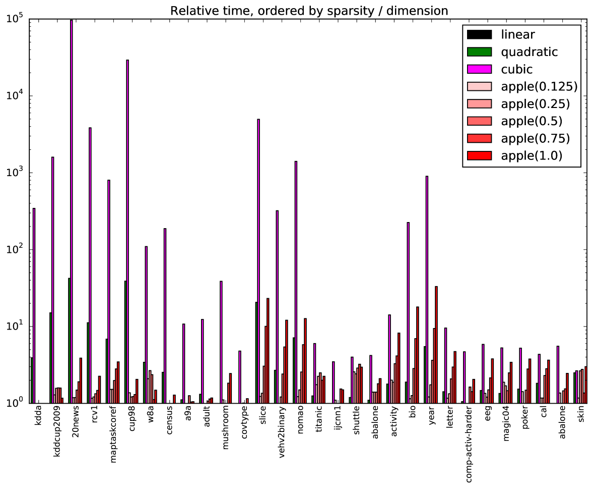
Since the statistical error by itself only tells half the story, we also include a similar plot for relative running times in Figure 6.

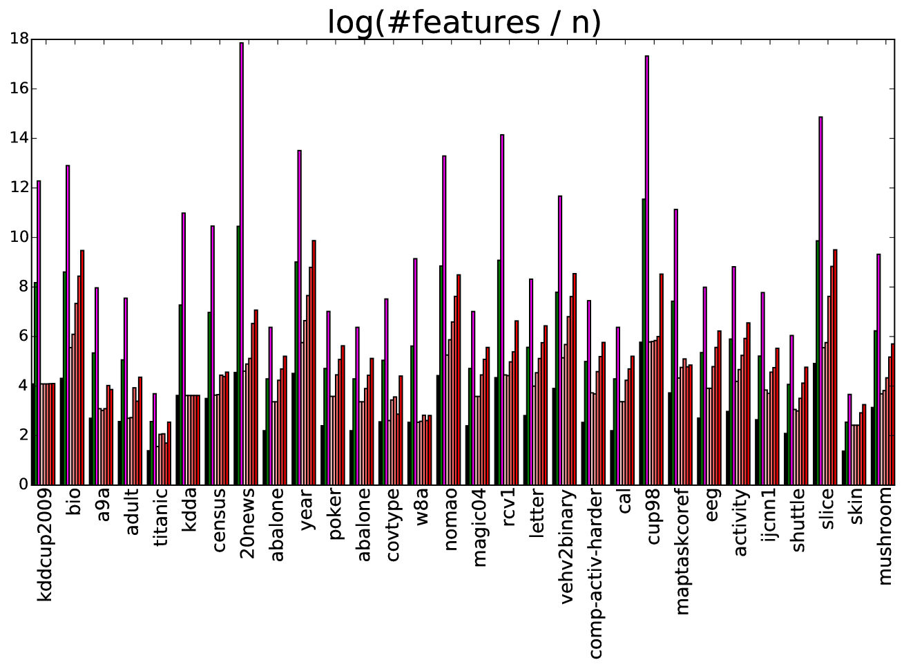
Finally, we also want to highlight that despite the competitive statistical performance, our adaptive methods indeed generate a much smaller number of monomials. To this end, we compute the average number of non-zero features per example on all datasets for all methods. These plots are presented in Figure 7, with the same color coding used for algorithms as the previous two plots.

We include tables with all the (non-relative) errors and times in Table 2 and Table 3.

Figure 5: Relative error plots for $\mathtt{apple}$ and baselines on all 30 datasets. Should be viewed in color.

Figure 6: Relative time plots for $\mathtt{apple}$ and baselines on all 30 datasets. Should be viewed in color.

Figure 7: Relative time plots for $\mathtt{apple}$ and baselines on all 30 datasets. Should be viewed in color.

	$\mathtt{lin}$	$\mathtt{quad}$	$\mathtt{cubic}$	$\mathtt{apple}$ (1)	$\mathtt{apple}$ (0.75)	$\mathtt{apple}$ (0.5)	$\mathtt{apple}$ (0.25)	$\mathtt{apple}$ (0.125)
bio	3.122e-03	3.122e-03	3.087e-03	2.985e-03	3.053e-03	2.985e-03	3.259e-03	3.156e-03
	2.644e+00	5.000e+00	5.965e+02	3.036e+00	3.340e+00	7.516e+00	1.841e+01	4.745e+01
a9a	1.510e-01	1.485e-01	1.496e-01	1.488e-01	1.488e-01	1.489e-01	1.478e-01	1.481e-01
	3.880e-01	4.320e-01	4.176e+00	2.840e-01	3.000e-01	4.880e-01	4.040e-01	4.080e-01
adult	1.557e-01	1.529e-01	1.531e-01	1.525e-01	1.525e-01	1.507e-01	1.513e-01	1.474e-01
	3.440e-01	4.520e-01	4.252e+00	2.480e-01	2.400e-01	3.680e-01	3.920e-01	4.040e-01
titanic	2.182e-01	2.136e-01	2.136e-01	2.136e-01	2.136e-01	2.136e-01	2.136e-01	2.136e-01
	1.600e-02	2.000e-02	9.601e-02	2.800e-02	3.600e-02	4.000e-02	3.200e-02	3.600e-02
kdda	1.240e-01	1.272e-01	1.253e-01	1.240e-01	1.240e-01	1.240e-01	1.240e-01	1.240e-01
	9.492e+01	3.715e+02	3.266e+04	7.629e+01	6.689e+01	8.318e+01	5.768e+01	8.463e+01
census	4.748e-02	4.579e-02	4.651e-02	4.674e-02	4.686e-02	4.698e-02	4.586e-02	4.648e-02
	3.068e+00	7.784e+00	5.754e+02	2.200e+00	2.180e+00	2.144e+00	2.532e+00	3.936e+00
20news	8.119e-02	8.437e-02	8.384e-02	8.437e-02	9.021e-02	1.210e-01	9.525e-02	7.986e-02
	5.440e-01	2.303e+01	5.262e+04	6.440e-01	6.480e-01	8.121e-01	1.040e+00	2.112e+00
abalone_bin	2.898e-01	2.826e-01	2.719e-01	2.874e-01	2.874e-01	2.766e-01	2.743e-01	2.754e-01
	4.400e-02	4.000e-02	2.440e-01	6.000e-02	4.400e-02	6.400e-02	6.800e-02	1.080e-01
year	1.157e-02	1.073e-02	1.113e-02	1.112e-02	1.099e-02	1.083e-02	1.069e-02	1.060e-02
	1.261e+01	6.915e+01	1.136e+04	1.529e+01	2.201e+01	4.585e+01	1.189e+02	4.179e+02
poker	4.555e-01	4.091e-01	4.100e-01	4.119e-01	4.119e-01	4.092e-01	4.099e-01	4.085e-01
	4.388e+00	6.736e+00	2.294e+01	6.228e+00	3.836e+00	6.516e+00	1.230e+01	1.657e+01
abalone_reg	8.052e+00	7.489e+00	7.107e+00	7.812e+00	7.812e+00	7.690e+00	7.003e+00	6.740e+00
	4.000e-02	4.400e-02	1.680e-01	5.600e-02	5.600e-02	5.600e-02	7.200e-02	8.400e-02
kddcup2009	7.310e-02	7.310e-02	7.310e-02	7.310e-02	7.310e-02	7.310e-02	7.310e-02	7.310e-02
	7.600e-01	1.144e+01	1.213e+03	9.801e-01	1.196e+00	1.208e+00	1.204e+00	8.881e-01
covtype	2.450e-01	2.184e-01	2.039e-01	2.331e-01	2.331e-01	2.287e-01	2.261e-01	2.208e-01
	4.444e+00	3.116e+00	2.133e+01	4.204e+00	4.488e+00	2.856e+00	5.120e+00	4.192e+00
w8a	1.538e-02	1.246e-02	1.337e-02	1.518e-02	1.518e-02	1.417e-02	1.317e-02	1.286e-02
	1.320e-01	4.520e-01	1.448e+01	2.760e-01	3.520e-01	3.120e-01	1.480e-01	1.960e-01
nomao	6.325e-02	5.063e-02	5.107e-02	5.992e-02	5.701e-02	5.513e-02	4.933e-02	4.904e-02
	5.000e-01	3.564e+00	7.038e+02	6.120e-01	7.480e-01	1.280e+00	2.900e+00	6.348e+00

Table 2: Errors (first row) and running time in seconds (second row) for each dataset for the baselines and $\mathtt{apple}$ variants (first 15 datasets).

	$\mathtt{lin}$	$\mathtt{quad}$	$\mathtt{cubic}$	$\mathtt{apple}$ (1)	$\mathtt{apple}$ (0.75)	$\mathtt{apple}$ (0.5)	$\mathtt{apple}$ (0.25)	$\mathtt{apple}$ (0.125)
magic04	2.142e-01	1.672e-01	1.638e-01	1.880e-01	1.880e-01	1.801e-01	1.706e-01	1.696e-01
	1.040e-01	1.400e-01	5.480e-01	1.960e-01	1.760e-01	1.520e-01	2.600e-01	3.560e-01
rcv1	4.860e-02	4.060e-02	3.701e-02	4.570e-02	4.511e-02	4.438e-02	4.273e-02	4.205e-02
	1.627e+01	1.823e+02	6.251e+04	1.895e+01	1.977e+01	2.171e+01	2.401e+01	3.671e+01
letter	2.273e-01	1.918e-01	1.688e-01	1.872e-01	1.878e-01	1.727e-01	1.670e-01	1.638e-01
	1.440e-01	2.040e-01	1.376e+00	1.680e-01	1.920e-01	3.000e-01	4.280e-01	6.800e-01
vehv2binary	3.400e-02	2.670e-02	2.505e-02	8.337e-03	8.087e-03	8.772e-03	1.109e-02	1.151e-02
	3.364e+00	9.065e+00	1.079e+03	2.880e+00	4.076e+00	8.105e+00	1.825e+01	4.065e+01
comp	3.409e-03	2.627e-03	3.662e-03	2.587e-03	2.587e-03	2.124e-03	2.038e-03	2.070e-03
	7.601e-02	8.000e-02	3.560e-01	6.401e-02	6.400e-02	1.240e-01	1.080e-01	1.560e-01
cal_housing	7.410e-02	8.651e-02	1.055e-01	9.414e-02	9.414e-02	9.856e-02	9.881e-02	1.183e-01
	9.201e-02	1.680e-01	4.000e-01	1.080e-01	1.080e-01	2.120e-01	2.600e-01	3.360e-01
cup98	5.697e-02	3.841e-02	4.215e-02	5.646e-02	5.687e-02	6.450e-02	6.780e-02	5.948e-02
	3.452e+00	1.342e+02	1.010e+05	4.736e+00	4.180e+00	4.240e+00	4.504e+00	7.084e+00
maptaskcoref	1.087e-01	7.553e-02	6.598e-02	9.997e-02	9.805e-02	9.691e-02	9.338e-02	8.083e-02
	9.361e-01	6.412e+00	7.504e+02	1.424e+00	1.424e+00	1.856e+00	2.628e+00	3.240e+00
eeg_eye_state	3.815e-01	2.573e-01	2.300e-01	3.127e-01	3.127e-01	2.557e-01	2.383e-01	2.136e-01
	1.360e-01	2.000e-01	7.960e-01	1.840e-01	1.640e-01	2.040e-01	2.920e-01	5.160e-01
activity	1.298e-02	8.422e-03	6.762e-03	8.694e-03	5.856e-03	5.977e-03	4.951e-03	4.166e-03
	5.560e-01	9.921e-01	7.864e+00	1.116e+00	1.048e+00	1.828e+00	2.304e+00	4.564e+00
ijcnn1	7.942e-02	4.501e-02	3.481e-02	5.221e-02	5.221e-02	4.041e-02	3.921e-02	3.901e-02
	2.000e-01	1.800e-01	6.960e-01	2.200e-01	1.800e-01	1.840e-01	3.080e-01	3.000e-01
shuttle	2.644e-02	1.391e-02	9.195e-03	1.218e-02	1.218e-02	5.402e-03	1.023e-02	7.931e-03
	1.040e-01	1.240e-01	4.160e-01	2.680e-01	2.520e-01	3.000e-01	3.360e-01	3.080e-01
slice	7.243e-03	1.403e-03	7.797e-04	5.095e-03	3.455e-03	2.302e-03	1.825e-03	1.196e-03
	1.600e+00	3.303e+01	7.944e+03	1.972e+00	2.168e+00	4.880e+00	1.609e+01	3.709e+01
skin	7.421e-02	1.045e-02	5.835e-03	2.165e-02	2.165e-02	2.165e-02	1.585e-02	7.366e-03
	4.600e-01	1.148e+00	1.220e+00	5.400e-01	1.220e+00	1.276e+00	6.280e-01	1.384e+00
mushroom	5.723e-02	5.538e-03	6.154e-04	6.646e-02	9.108e-02	4.923e-02	1.538e-02	1.846e-02
	7.200e-02	6.800e-02	2.788e+00	8.001e-02	5.600e-02	6.000e-02	1.320e-01	1.760e-01

Table 3: Errors (first row) and running time in seconds (second row) for each dataset for the baselines and $\mathtt{apple}$ variants (last 15 datasets).

References

- [1] Alekh Agarwal, Olivier Chapelle, Miroslav Dudík, and John Langford. A reliable effective terascale linear learning system. Journal of Machine Learning Research, 15(Mar):1111–1133, 2014.
- [2] Alexandr Andoni, Rina Panigrahy, Gregory Valiant, and Li Zhang. Learning sparse polynomial functions. In SODA, 2014.
- [3] Avrim Blum, Adam Kalai, and John Langford. Beating the hold-out: Bounds for k-fold and progressive cross-validation. In COLT, 1999.
- [4] Antoine Bordes, Seyda Ertekin, Jason Weston, and Léon Bottou. Fast kernel classifiers with online and active learning. Journal of Machine Learning Research, 6:1579–1619, 2005.
- [5] Sébastien Bubeck. Theory of convex optimization for machine learning. 2014. arXiv:1405.4980 [math.OC].
- [6] Alexandros G. Dimakis, Adam Klivans, Murat Kocaoglu, and Karthikeyan Shanmugam. A smoothed analysis for learning sparse polynomials. CoRR, abs/1402.3902, 2014.
- [7] John Duchi, Elad Hazan, and Yoram Singer. Adaptive subgradient methods for online learning and stochastic optimization. The Journal of Machine Learning Research, 12:2121–2159, 2011.
- [8] Yoav Freund and Robert E. Schapire. A decision-theoretic generalization of on-line learning and an application to boosting. Journal of Computer and System Sciences, 55(1):119–139, 1997.
- [9] Jerome H. Friedman. Greedy function approximation: A gradient boosting machine. Technical report, Department of Statistics, Stanford University, 1999.
- [10] K. Hall, S. Gilpin, and G. Mann. Mapreduce/bigtable for distributed optimization. In Workshop on Learning on Cores, Clusters, and Clouds, 2010.
- [11] Raffay Hamid, Alex Gittens, Ying Xiao, and Dennis Decoste. Compact random feature maps. In ICML, 2014.
- [12] A. G. Ivakhnenko. Polynomial theory of complex systems. Systems, Man and Cybernetics, IEEE Transactions on, SMC-1(4):364–378, 1971.
- [13] Rie Johnson and Tong Zhang. Learning nonlinear functions using regularized greedy forest. Pattern Analysis and Machine Intelligence, IEEE Transactions on, 36(5):942–954, May 2014.
- [14] Adam Tauman Kalai, Alex Samorodnitsky, and Shang-Hua Teng. Learning and smoothed analysis. In FOCS, 2009.
- [15] Purushottam Kar and Harish Karnick. Random feature maps for dot product kernels. In AISTATS, 2012.
- [16] Nikos Karampatziakis and John Langford. Online importance weight aware updates. In UAI, pages 392–399, 2011.
- [17] Michael W. Mahoney. Randomized algorithms for matrices and data. Foundations and Trends in Machine Learning, 3(2):123–224, 2011.
- [18] H. Brendan McMahan and Matthew J. Streeter. Adaptive bound optimization for online convex optimization. In COLT, pages 244–256, 2010.
- [19] Indraneel Mukherjee, Kevin Canini, Rafael Frongillo, and Yoram Singer. Parallel boosting with momentum. In Proceedings of the European Conference on Machine Learning and Principles and Practice of Knowledge Discovery in Databases, 2013.
- [20] Ninh Pham and Rasmus Pagh. Fast and scalable polynomial kernels via explicit feature maps. In Proceedings of the 19th ACM SIGKDD International Conference on Knowledge Discovery and Data Mining, 2013.
- [21] Ali Rahimi and Benjamin Recht. Random features for large-scale kernel machines. In Advances in Neural Information Processing Systems 20, 2008.
- [22] Stéphane Ross, Paul Mineiro, and John Langford. Normalized online learning. In UAI, 2013.
- [23] Terence D. Sanger, Richard S. Sutton, and Christopher J. Matheus. Iterative construction of sparse polynomial approximations. In Advances in Neural Information Processing Systems 4, 1992.
- [24] Bernhard Schölkopf and Alexander Smola. Learning with Kernels. MIT Press, Cambridge, MA, 2002.
- [25] Ohad Shamir and Tong Zhang. Stochastic gradient descent for non-smooth optimization: Convergence results and optimal averaging schemes. In ICML, 2013.
- [26] R. Tibshirani. Regression shrinkage and selection via the lasso. J. Royal. Statist. Soc B., 58(1):267–288, 1996.
- [27] J. A. Tropp and A. C. Gilbert. Signal recovery from random measurements via orthogonal matching pursuit. IEEE Transactions on Information Theory, 53(12):4655–4666, December 2007.
- [28] Christopher Williams and Matthias Seeger. Using the Nyström method to speed up kernel machines. In Advances in Neural Information Processing Systems 13, 2001.
- [29] Martin Zinkevich. Online convex programming and generalized infinitesimal gradient ascent. In ICML, 2003.