Burchnall-Chaundy polynomials and the Laurent phenomenon
A.P. Veselov
Department of Mathematical Sciences,
Loughborough University, Loughborough LE11 3TU, UK and Moscow State University, Moscow 119899, Russia
A.P.Veselov@lboro.ac.uk and R. Willox
Graduate School of Mathematical Sciences, The University of
Tokyo,
3-8-1 Komaba, Meguro-ku, Tokyo 153-8914
willox@ms.u-tokyo.ac.jp
Abstract.
The Burchnall-Chaundy polynomials
are determined by the differential recurrence relation
with The fact that this recurrence relation has all solutions polynomial is not obvious
and is similar to the integrality of Somos sequences and the Laurent phenomenon.
We discuss this parallel in more detail and extend it to two difference equations
and
related to two different KdV-type reductions of the Hirota-Miwa
and Dodgson octahedral equations. As a corollary we have a new form of the Burchnall-Chaundy polynomials in terms of the initial data , which is shown to be Laurent.
1. Introduction
In the 1920s Burchnall and Chaundy [5] discovered a remarkable sequence of polynomials satisfying the recurrence relation
(1)
with , where ′ means differentiation in :
Note that at each step we have an additional integration constant because of the freedom in the solution of the differential equation
(we are using here Adler and Moser’s notation with , see [2]).
These polynomials have been rediscovered several times, most notably by Stellmacher and Lagnese in the theory of Huygens’ principle [19]
and by Adler and Moser in the theory of rational solutions of the Korteweg-de Vries equation [2]. They appeared also in the bispectral theory of Duistermaat and Grünbaum [8], who explained their important role in the theory of monodromy-free Schrödinger operators and the relation to Schur polynomials with triangular Young diagrams.
The Burchnall-Chaundy polynomials are special cases of the Schur-Weierstrass polynomials introduced by Buchstaber, Enolskii and Leykin in the theory of Klein sigma-functions [3] (see also Nakayashiki [16] for the relation to KP tau functions and Sato theory).
Note that the very existence of these polynomials looks like a miracle since the relation (1) can be rewritten as
which means that all the residues of the right-hand side must be zero (see the discussion of this in [5] and [2]).
We would like to make the parallel with the sequence
which surprisingly is integer for all : (these in fact are nothing else but every other Fibonacci number).
This sequence is related to the cluster algebra of type and gives a nice example of the so-called Laurent phenomenon studied by Fomin and Zelevinsky:
for general initial data and , the solution is a Laurent polynomial in and with integer coefficients (see [6, 9]).
In particular, if this implies the integrality of the (which, of course, can be proven in an elementary way as well).
We see that the Burchnall-Chaundy sequence is a functional analogue of the same phenomenon with the role of integers played by the polynomial ring
This work started as an attempt to see if this conceptual parallel with the Laurent phenomenon can be made a real connection.
This led us naturally to the following difference Burchnall-Chaundy equation
(2)
with
We prove that this equation also has polynomial solutions with coefficients that are Laurent polynomials of the initial data
, such that
where
The first three polynomials have the form
If we set , the difference Burchnall-Chaundy equation simply becomes
a certain KdV-type reduction of the Hirota-Miwa equation, which is known to have the Laurent property [9].
This explains the Laurent property of the coefficients,
but the proof of polynomiality of needs additional arguments and is related
to specific properties of the Cauchy problem we consider.
We follow here the classical approach [5], [2] by using an explicit description of solutions
in terms of Casorati determinants, which are standard in the theory of integrable systems.
As a result we obtain an independent proof of the Laurent property for the coefficients and a recursive way for their calculation.
We show also that these polynomials, after rescaling ,
satisfy the difference equation
(3)
with the same initial data
This equation, which we call difference Dodgson equation, for is a reduction of the 3D Dodgson octahedral equation,
which is formally equivalent to the Hirota-Miwa equation but has different geometry.
We show that under a natural continuum limit the polynomials become the usual Burchnall-Chaundy polynomials
thus giving one more proof for their existence.
A corollary of our results is the proof that in terms of the initial data ,
have coefficients which are Laurent polynomials in with integer coefficients:
This form of the Burchnall-Chaundy polynomials seems to be new and demonstrates one more feature of these remarkable polynomials.
2. Dodgson, Hirota-Miwa and Burchnall-Chaundy
In 1866 Charles Dodgson (known to the world under the name of Lewis Carroll) proposed a very original method of computing determinants called “condensation method” [7].
One can view this method as the solution of a very special Cauchy problem for the discrete Dodgson octahedral equation
(4)
where Let be an matrix for which the determinant is to be computed. Assume that is odd and consider the following Cauchy data: for all , and
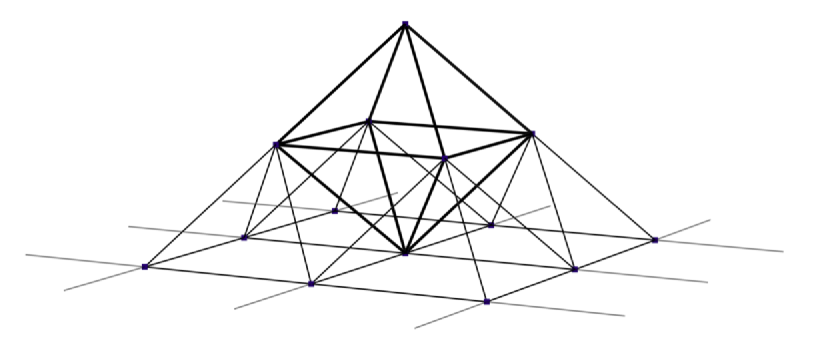
when and otherwise. For even we should consider the same initial data for and respectively. The Dodgson condensation can be viewed as the evolution, according to (4), along the positive -direction inside the characteristic cone: . The support of such a solution for a generic matrix will therefore be a pyramid with matrix in the base and the determinant at the top (see Fig.1). Outside this pyramid we can assume all for to be zero such that the equation is trivially satisfied.
Figure 1. Dodgson’s Cauchy pyramid for computing determinants
In the 1980s Hirota [11] discovered a discrete version of the KP equation on a standard cubic lattice, which was subsequently studied by Miwa [15] in relation to Sato theory, and which is now known as the Hirota-Miwa equation
(5)
where and are arbitrary non-zero parameters. Note that the exact values of the parameters are not very important and can be changed by the gauge transformation
which however will affect the Cauchy data.
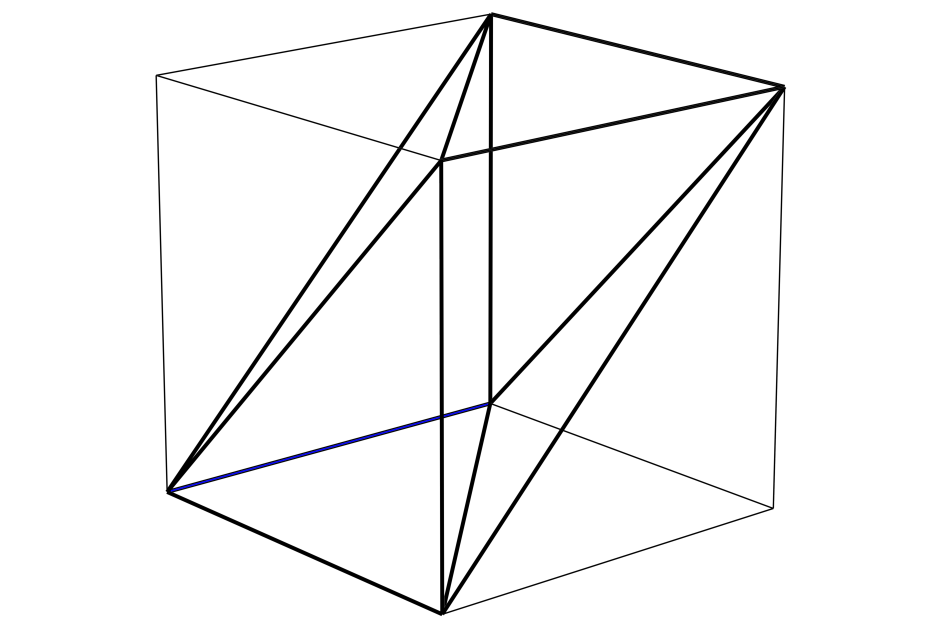
Formally the Hirota-Miwa equation may be considered as a version of the Dodgson equation if one interprets these six vertices of the cube
as the vertices of the octahedron, see Figure 2.
Figure 2. Support of the Hirota-Miwa equation in the cube
It is however clear that from a geometric point of view this is unnatural.
Indeed, the typical initial value problems for the Hirota-Miwa equation
are very different from the Dodgson initial value problem. In particular, typical explicit solutions for the Hirota-Miwa equation are given by determinants of the same size, while for Dodgson it is crucial that the size of the matrices is shrinking when moving up in the pyramid.
This difference is clear if we compare two natural reductions of these equations.
For the octahedral equation we consider the reduction leading to the discrete Dodgson equation
(6)
where If we extend this equation to all integers and replace by we come to the difference
Dodgson equation (3).
For Hirota-Miwa a natural reduction is which, for , leads to the discrete KdV equation in Hirota bilinear form [10]
(7)
the functional version of which is the Burchnall-Chaundy equation (2). Note that the support of the equation has a domino shape, which is a cube squashed along one of the face diagonals, see Figure 3.
Figure 3. Domino-type support for the discrete KdV equation.
Because of their common origin it is natural to expect that the equations (2) and (3) are closely related, which is indeed the case.
Theorem 1.
The difference Burchnall-Chaundy (2) and Dodgson (3) equations
are equivalent on the set of initial data satisfying where
(8)
More precisely, if the initial data of the Cauchy problem for the dBCh equation (2)
satisfy the constraint
then we simply have to show that under the constraint we have
Note that the constraint is preserved by the Burchnall-Chaundy dynamics. Indeed, assume that
Now in order to prove that the satisfy (10), we multiply relation (11) by , (12) by , (13) by and add all of them to obtain
Dividing now by proves the claim.
∎
This theorem can be reformulated as follows. Consider a two by two square formed by two adjacent KdV dominos (see Figure 3). It can be alternatively described as two horizontal dominos with relations and on them. Then the claim is that any three of these domino relations implies the fourth one and the Dodgson relation (10).
3. Cauchy problem for discrete equations and Laurent property
Fomin and Zelevinsky [9] have shown that the Hirota-Miwa and the octahedral Dodgson equations have the Laurent property
for suitable initial data. They also considered some reductions, including the discrete KdV equation
(15)
(which they called ”the knight recurrence” and attributed to Noam Elkies).
In the case of a particular Cauchy problem for this equation with and
this implies that the general solution is a Laurent polynomial in with integer coefficients.
In particular, this implies that when all , all the are integers as can be seen in Figure 4.
Figure 4. Solution to the discrete KdV equation with Cauchy data . The axes are given by the column of 1’s ( axis) and the top row of 1’s ( axis).
Note that on the line in this figure we have the Fibonacci numbers ,
which grow like , where is the
golden ratio. On the next line we have the sequence satisfying the linear recurrence,
with Fibonacci numbers as the coefficients, which grows like Similarly, for fixed grows exponentially like as
In the direction the growth is much slower: for fixed the grow like
This indicates that the dependence on is polynomial, but to prove this for arbitrary initial data seems to be not easy.
Instead we prefer to use (like Burchnall and Chaundy [5] and Adler and Moser[2]) alternative tools, standard in the theory of integrable systems, by presenting explicit determinantal expressions for the solutions. The Wronskians from [2, 5] are naturally replaced by Casoratians in our case, which is usual in the discrete setting, see e.g. [17]. Note however that in soliton KP theory, the matrices that yield determinant solutions usually have the same size, which for example in the case of the discrete KdV equation (15) would require the sum of the coefficients and to be equal to 1. This is not true in our case (7), for which it is known [2, 5] that it is essential to have matrices of growing size.
4. Casorati determinantal formulae
Let be a solution of the Cauchy problem for the difference Burchnall-Chaundy equation (2)
with Cauchy data and arbitrary values for
Since the Cauchy data satisfy the constraint (9)
the corresponding polynomials
that satisfy (3) are simply
The following procedure is a natural difference analogue of the Adler and Moser description of Burchnall-Chaundy polynomials [2].
Define first the sequence of polynomials by
(16)
where
They depend on some additional parameters, which are not unique.
The generating function
satisfies the
relation
and has the general form
where is an arbitrary function of the parameters.
We fix the choice of these parameters, which will turn out to be related to the KdV flows, by choosing
so that
(17)
leading to
These polynomials can be given also as the determinants (see e.g. [12], page 28)
(18)
Let now and consider the
Casoratians , where the Casoratian
of the functions is defined as
(19)
The Casoratians
(20)
can be written as the determinants
(21)
Theorem 2.
The Casoratians given by (21) with defined by (18) satisfy the Burchnall-Chaundy relations (2).
Proof.
We essentially follow the arguments of Adler and Moser [2].
Let be arbitrary functions of and consider
the difference operator
Then we have what Adler and Moser call Jacobi identity:
where
is the shift operator:
and by we mean the Casoratian of and
The proof is simple: both and are difference operators
of order with the same kernel generated by .
Thus they can only differ by a factor, which is easily seen to be .
In our case we have and
It is then easy to see that this implies that if we take then
However,
and similarly: . Substituting this into the Jacobi identity
we have
Note that the initial conditions are homogeneous in of weight .
Theorem 3.
The polynomial depends only on odd parameters
and has the form
for some polynomials with rational coefficients.
The parameter can be expressed in terms of as a Laurent polynomial with integer coefficients
Proof.
The generating function (17) satisfies the differential relations
which imply that
Differentiating the determinantal expression (21) with respect to we see that the derivative of the -th column is precisely the preceding column and consequently, as the derivative of the first column is zero, that does not depend on . Similarly we see that the same is true for all even times (cf. [3]).
This means that we can choose the even times as we want. Let us choose them in such a way that the corresponding for all
This then defines the as certain polynomials of odd times with rational coefficients:
From the determinant (21) we see that in this case the satisfy the recurrence relation
for some polynomial with integer coefficients, which implies the first claim. This relation also allows us to express,
recursively, (and hence using (22)) as a Laurent polynomial of with integer coefficients.
∎
The first four expressions for the have the form:
Combining the expression (21) for with the previous theorem we have
Corollary 2.
Laurent phenomenon for the Burchnall-Chaundy sequence (2):
The first three polynomials are given explicitly in the Introduction.
The polynomials corresponding to zero Cauchy data
have to be dealt with as a special case because of the Laurent nature of the solution. Instead we can consider their expressions in terms of the , which are polynomial, and therefore allow us to set .
The corresponding polynomials admit the following explicit description.
Define the polynomials
by the following recurrence relation
(23)
or explicitly as
(24)
where and denotes the integer part of
Theorem 4.
The polynomials satisfy the difference Burchnall-Chaundy relations with zero initial data
Proof is by a direct check.
The polynomials correspond to all and thus have Casoratian form (20) with
binomial
It is interesting that they also can be given as symmetric Casoratians of simple monomials.
The symmetric Casoratian of the functions is defined as the determinant
(25)
Define the functions
(26)
Theorem 5.
The polynomials can be given as the symmetric Casoratians
It is well-known [1, 2] that the Burchnall-Chaundy polynomials are the -functions of the rational solutions of the
Korteweg-de Vries equation
and its higher analogues
(see [14], where these equations are precisely defined for scaled ). Namely, in a proper parametrisation
are the general rational solutions of the KdV hierarchy [1, 2].
Adler and Moser realised that the parameters they used (see the formulae in the Introduction) are different from the KdV times
but are related to them by a non-trivial invertible polynomial transformation.
We claim that our parameters are simply related to the KdV times by
the scaling
Theorem 6.
The continuum limit
yields the usual Burchnall-Chaundy polynomials parametrized by the scaled KdV times
Note that is polynomial in because of the homogeneity property of the ’s. The proof then follows from Miwa’s results on the relation between the Hirota-Miwa equation and KP/KdV hierarchy [15]
and by comparison with the normalisation of the KdV flows in [14].
Since the initial data are homogeneous in they do not change during the continuum limit and we have
Corollary 3.
Laurent phenomenon for the usual Burchnall-Chaundy relation (1):
The explicit form of the first 4 polynomials is given in the Introduction.
6. Concluding remarks
The main question we are dealing with in this paper is basically what happens with the Laurent property when we replace a discrete equation by its functional difference version. Our point is that the answer depends very much on the type of the corresponding Cauchy problem.
It is known to the experts in integrable systems that the equation itself does not guarantee integrability,
which holds only for particular initial value problems and functional class of the initial data.
For example, for the KdV equation the initial value problem is integrable for decaying or periodic initial data [18],
but for general initial data not much can be said.
At the discrete level this fact is less visible and the importance of the choice of Cauchy problem is probably not well recognised. A discussion of the role the Cauchy problem plays with respect to the Laurent phenomenon for integrable equations can be found in [13].
To illustrate our point let us consider the same discrete KdV dynamics (7), but in the direction, and its
functional version by replacing by :
with It has the explicit solutions ,
but these correspond to particular Cauchy data satisfying
What can one say about the analytic structure of the solutions for general Cauchy data (in particular, for ) ? So, in other words, what are the analytic functions interpolating integers on the vertical lines in Figure 4 ?
It is clear that the case of the Burchnall-Chaundy polynomials is special, but the question is how special it is.
It would be interesting therefore to study other reductions, in particular period 3 reductions which correspond to the Boussinesq equation and which should be related to Schur-Weierstrass polynomials for trigonal curves [3]. It is natural to link this with the theory of periodic Darboux/dressing chains [20, 21].
It would also be interesting to know if the polynomials play any special role
in the theory of hyperelliptic sigma-functions [4].
7. Acknowledgements
A.P.V. is grateful to the Graduate School of Mathematical Sciences of the University of Tokyo
for the support of his visit in April-July 2014, during which this work was done.
R.W. would like to acknowledge support from the Japan Society for the Promotion of Science,
through the JSPS grant: KAKENHI 24540204.
References
[1]
H. Airault, H.P. McKean and J. Moser Rational and elliptic solutions of
the Korteweg-de Vries equation and a related many-body problem.
Comm. Pure Appl. Math. 30 (1977), 95–178.
[2]
M. Adler and J. Moser On a class of polynomials connected with the Korteweg-de Vries equation.
Commun. Math. Phys., 61 (1978), 1–30.
[3]
V.M. Buchstaber, V.Z. Enolskii and D.V. Leykin Rational analogs of abelian functions.
Funct. Anal. Appl., 33 (1999), 83-94.
[4]
V.M. Buchstaber, V.Z. Enolskii and D.V. Leykin Kleinian functions, hyperelliptic Jacobians and applications. Reviews in Math. and Math. Phys. 10 (1997), 1–125.
[5]
J.L. Burchnall and T.W. Chaundy A set of differential equations which
can be solved by polynomials. Proc. London Math. Soc.
30 (1929-30), 401–414.
[6]
P. Caldero and A. Zelevinsky Laurent expansions in cluster algebras via quiver
representations. Moscow Mathematical Journal
6, no. 3 (2006), 411–429.
[7]
C.L. Dodgson Condensation of determinants, being a new and brief method
for computing their arithmetical values. Proc. Royal Soc. London 15 (1886-67), 150–155.
[8]
J.J. Duistermaat and F.A. Grünbaum Differential equations in the spectral parameter.
Comm. Math. Phys. 103, no. 2 (1986), 177–240.
[9]
S. Fomin and A. Zelevinsky The Laurent Phenomenon.
Adv. Appl. Math. 28 (2002), 119–144.
[10]
R. Hirota Nonlinear partial difference equations. I. A difference analogue of the Korteweg-de Vries equation. J. Phys. Soc. Japan 43 (1977), 1424–1433.
[11]
R. Hirota Discrete analogue of a generalised Toda equation. J. Phys. Soc. Japan 50 (1981), 3787–3791.
[12]
I.G. Macdonald Symmetric functions and Hall polynomials. 2nd edition, Oxford Univ. Press, 1995.
[13]
T. Mase The Laurent phenomenon and discrete integrable systems. RIMS Kokyuroku Bessatsu B41 (2013), 43–64.
[14]
R. M. Miura, C. S. Gardner and M. D. Kruskal Korteweg-de-Vries equation and generalizations V. J. Math. Phys. 11 (3) (1970), 952–953.
[15]
T. Miwa On Hirota’s difference equation. Proc. Japan Acad. A 58 (1982), 9–12.
[16]
A. Nakayashiki Sigma function as a tau function. IMRN 2010 (2009), 383–394.
[17]
Y. Ohta, R. Hirota, S. Tsujimoto and T. Imai Casorati and discrete Gram type determinant representations of solutions to the discrete KP hierarchy. J. Phys. Soc. Japan 62 (1993), 1872–1886.
[18]
S.P. Novikov, S.V. Manakov, L.P. Pitaevskiĭ and V.E. Zakharov. Theory of solitons: The inverse scattering method.
Plenum, New York, 1984.
[19]
J.E. Lagnese and K.L. Stellmacher A method of generating classes of Huygens’
operators. J. Math. & Mech. 17 (1967), 461–472.
[20] A.P. Veselov and A.B. Shabat Dressing chains and the spectral theory of the Schrödinger operator Funct. Anal.
Appl. 27 (1993), 81–96.
[21]
R. Willox and J. Satsuma Sato Theory and Transformations Groups. A Unified Approach to Integrable Systems in Discrete Integrable Systems, B. Grammaticos, Y. Kosmann-Schwarzbach, Tamizhmani, Tamizharasi (Eds.), Springer-Verlag Berlin (2004), 17–55.