Ion-temperature-gradient sensitivity of the hydrodynamic instability caused by shear in the magnetic-field-aligned plasma flow

Abstract

The cross-magnetic-field (i.e., perpendicular) profile of ion temperature and the perpendicular profile of the magnetic-field-aligned (parallel) plasma flow are sometimes inhomogeneous for space and laboratory plasma. Instability caused by a gradient in either the ion-temperature profile or by shear in the parallel flow has been discussed extensively in the literature. In this paper, hydrodynamic plasma stability is investigated, real and imaginary frequency are quantified over a range of the shear parameter, the normalized wavenumber, and the ratio of density-gradient and ion-temperature-gradient scale lengths, and the role of inverse Landau damping is illustrated for the case of combined ion-temperature gradient and parallel-flow shear. We find that increasing the ion-temperature gradient reduces the instability threshold for the hydrodynamic parallel-flow shear instability, also known as the parallel Kelvin-Helmholtz instability or the D’Angelo instability. We also find that a kinetic instability arises from the coupled, reinforcing action of both free-energy sources. For the case of comparable electron and ion temperature, we illustrate analytically the transition of the D’Angelo instability to the kinetic instability as the shear parameter, the normalized wavenumber, and the ratio of density-gradient and ion-temperature-gradient scale lengths are varied and we attribute the changes in stability to changes in the amount of inverse ion Landau damping. We show that, near a normalized wavenumber $k_{\perp}\rho_{i}$ of order unity, the real and imaginary values of frequency become comparable and the growth rate maximizes.

I INTRODUCTION

Shear in magnetic-field-aligned (i.e., parallel) plasma flow can be found in spaceAmatucci ; Kintner ; McFadden , fusionAsakura ; LaBombard ; Fedorczak ; Pedrosa ; Wang and laboratoryAgrimson1 ; Koepke2002 ; Koepke2003 ; Koepke2004 ; Koepke2006 ; Sen ; Kaneko-03 ; Kaneko-05 plasma. Ionospheric regions of inhomogeneous parallel plasma flow can map magnetically to magnetospheric regions of large-scale field-aligned currents, resulting in broadband electrostatic noise in the auroral zone of geospace Amatucci .

Experimental observations from a number tokamaks and stellaratorsAsakura ; LaBombard ; Fedorczak ; Pedrosa ; Wang have found large nearly sonic parallel sheared flows inside the last closed flux surface. Near-sonic parallel sheared flows are systematically observed in the far scrape-off layer (SOL) of the X-point divertor tokamaks JT-60Asakura and Alcator C–Mod LaBombard tokamaks, in the limiter tokamak Tore SupraFedorczak . These flows are deemed unstableMcCarthy ; Garbet ; Schwander against the development of the well known hydrodynamic D’Angelo instability D'Angelo . Schwander et al.Schwander showed that plasma might be unstable to the parallel-flow shear instability around limiters, as inferred from the experimental findings of Fenzi et al.Fenzi , thereby explaining local enhancements of turbulence and showing that, according to the local linear stability criterion, stability is sensitive to core parallel rotation. Their work speaks to the interest that would be given to future numerical modelling of experimentally relevant plasma conditions to assess both the properties of the transport coefficients associated with the parallel-flow shear-driven instability and the presence of free-energy that would support turbulence that arises from that instability. In this paper, using analytical theory and numerical analysis, we quantify the real and imaginary frequency of the parallel-flow shear-driven instability over a range of the shear parameter, the normalized wavenumber, and the ratio of density-gradient and ion-temperature-gradient scale lengths and demonstrate that the flow-shear threshold for instability reduces as the ion-temperature gradient increases. We also illustrate the role of inverse Landau damping in this case of combined ion-temperature gradient and parallel-flow shear.

If the parallel-ion-flow shear is accompanied by inhomogeneous ion temperature, a hydrodynamic instability can develop into a kinetic instability as will be shown. The investigation of plasma stability in the presence of these two free-energy sources was initiated by S.Migliuolo in his investigations of the plasma sheet boundary layerMigliuolo in the Earth’s magnetosphere. He found, that kinetic instability arises by virtue of the coupled action of both parallel-velocity shear $V^{\prime}_{0}(x)$ and an ion temperature gradient that reinforce each other. Inverse ion Landau damping is responsible for the combined ion-temperature-gradient flow-shear-driven (ITG-FSD) kinetic instability, a conclusion quite different from D’Angelo’s conclusion for the homogeneous-temperature, hydrodynamic FSD instability in the framework of the two-fluid equations. The calculations in Ref. Migliuolo involved taking the large argument ($z_{i}=\omega/\sqrt{2}k_{z}v_{Ti}\gg 1$) limit of the ion plasma dispersion function and examining marginal stability, without quantifying the maximum growth rate. The linear analysis of the parallel-flow shear stability in the presence of inhomogeneous ion temperature with application to the edge tokamak plasma was performed in Ref.Rogister . It was predicted, that the roles of magnetic shear, trapped electrons, and toroidal curvature are negligible for the ITG–SFD kinetic instability and the behavior of the unstable growth rate was calculated only in the neighborhood of marginal instability.

In this paper, we present results from a numerical and analytical investigation of the sensitivity of the hydrodynamic D’Angelo mode to the ion temperature gradient and we interpret the transition of the hydrodynamic instability to the ITG–SFD kinetic instability. Extending beyond the result for marginal stability of Ref.Rogister , we arrive at the approximate analytical solution of the dispersion relation for the parameters associated with the maximum value of the growth rate.

The paper is organized as follows: The basic equations are presented in Sec.II. In Section III, we analyze the effect of the finite ion temperature and ion temperature gradient on the hydrodynamic D’Angelo mode. In Section IV, we consider the ITG–SFD kinetic instability. The Conclusions are presented in Sec.V.

II BASIC EQUATIONS

We consider a kinetic Vlasov-Poisson model of inhomogeneous, magnetic-field-aligned, single-ion-species, plasma flow with velocity ${\bf{V}}_{0}(X_{\alpha})\parallel toB_{0}{\bf{e}}_{z}$. The Vlasov equation for the perturbation $f_{\alpha}=F_{\alpha}-F_{0\alpha}$ of the distribution function $F_{\alpha}$ with equilibrium function $F_{0\alpha}$ in guiding center coordinates in slab geometry, $X_{\alpha}=x+\frac{v_{\bot}}{\omega_{c\alpha}}\sin\phi$, $Y_{\alpha}=y-\frac{v_{\bot}}{\omega_{c\alpha}}\cos\phi$, where $\omega_{c\alpha}$ is the cyclotron frequency, has a form

$$\displaystyle\frac{\partial f_{\alpha}}{\partial t}-\omega_{c}\frac{\partial f_{\alpha}}{\partial\phi}+v_{z}\frac{\partial f_{\alpha}}{\partial z}$$

$$\displaystyle=\frac{e}{m\omega_{c}}\frac{\partial\Phi}{\partial Y}\frac{\partial F_{0\alpha}}{\partial X}-\frac{e}{m}\frac{\omega_{c}}{v_{\bot}}\frac{\partial\Phi}{\partial\phi}\frac{\partial F_{0\alpha}}{\partial v_{\bot}}+\frac{e}{m}\frac{\partial\Phi}{\partial z}\frac{\partial F_{0\alpha}}{\partial v_{z}}.$$ (1)

In what follows, $F_{i0}$ is considered as the shifted Maxwellian distribution function for electrons and ions ($\alpha=i,e$)

$$\displaystyle F_{0\alpha}=\frac{n_{0\alpha}\left(X_{\alpha}\right)}{\left({2\pi v_{T\alpha}^{2}}\right)^{3/2}}\exp\left[-\frac{v_{\perp}^{2}}{2v_{T\alpha}^{2}}-\frac{\left(v_{z}-V_{0}(X_{\alpha})\right)^{2}}{2v_{T\alpha}^{2}}\right],$$ (2)

assuming the inhomogeneity direction of the density and temperature of the sheared-flow species is along coordinate $X_{\alpha}$, $v_{T\alpha}=\left(T_{\alpha}\left(X_{\alpha}\right)/m_{\alpha}\right)^{1/2}$ is the thermal velocity. The flow velocity of ions $\mathbf{V}_{0}$ is assumed to be equal to that of the electrons which is consistent with the fluid approximation used for the Kelvin-Helmholtz instability but inconsistent with including the development of current-driven instabilities. In order to simplify the problem, a velocity $\mathbf{v}$ usually transforms from the laboratory to a convecting frame of reference, $\mathbf{v}=\hat{\mathbf{v}}+V_{0}(X_{\alpha})\mathbf{e}_{z}$. We consider here the idealized inhomogeneous-flow case of homogeneous parallel-velocity shear, i.e. $V^{\prime}_{0}=const$. After transformation, the Vlasov equation takes the form

$$\displaystyle\frac{\partial f_{\alpha}}{\partial t}-\omega_{c}\frac{\partial f_{\alpha}}{\partial\phi}+\left(\hat{v}_{z}+V_{0}(X_{\alpha})\right)\frac{\partial f_{\alpha}}{\partial z}$$

$$\displaystyle=\frac{e}{m\omega_{c}}\frac{\partial\Phi}{\partial Y}\left(\frac{\partial F_{0\alpha}}{\partial X}-V^{\prime}_{0}\frac{\partial F_{0\alpha}}{\partial\hat{v}_{z}}\right)$$

$$\displaystyle-\frac{e}{m}\frac{\omega_{c}}{v_{\bot}}\frac{\partial\Phi}{\partial\phi}\frac{\partial F_{0\alpha}}{\partial v_{\bot}}+\frac{e}{m}\frac{\partial\Phi}{\partial z}\frac{\partial F_{0\alpha}}{\partial v_{z}}.$$ (3)

The general approach to solving Eq.(3) is a Fourier transform over time and space coordinates employing the local approximation, for which restrictions $k_{x}L_{n}\gg 1$, $k_{x}L_{T_{i}}\gg 1$ and $k_{x}L_{v}\gg 1$ are assumed, where $L_{n}=\left[d\ln n_{0}\left(X\right)/dx\right]^{-1}$, $L_{T_{i}}=\left[d\ln T_{i}\left(X\right)/dx\right]^{-1}$ and $L_{v}=\left[d\ln V_{0}\left(X\right)/dx\right]^{-1}$. Although the local approximation is typically justifiable in the case of inverse electron Landau damping in homogeneous plasma, justification of the local approximation in the case of velocity shear $V^{\prime}_{0}$ having a value comparable to the ion cyclotron frequency requires careful and convincing arguments.

After the Fourier transformation over the space coordinates, Eq.(3) becomes

$$\displaystyle\frac{\partial f_{\alpha}}{\partial t}-\omega_{c}\frac{\partial f_{\alpha}}{\partial\phi}+ik_{z}\hat{v}_{z}f_{\alpha}\left(v_{\bot},\phi,\mathbf{k},t\right)-V^{\prime}_{0}k_{z}\frac{\partial f_{\alpha}}{\partial k_{x}}$$

$$\displaystyle=\frac{e}{m\omega_{c}}ik_{y}\Phi\left(\mathbf{k},t\right)\left(\frac{\partial F_{0\alpha}}{\partial X}-V^{\prime}_{0}\frac{\partial F_{0\alpha}}{\partial\hat{v}_{z}}\right)$$

$$\displaystyle-\frac{e}{m}\frac{\omega_{c}}{v_{\bot}}\frac{\partial\Phi}{\partial\phi}\frac{\partial F_{0\alpha}}{\partial v_{\bot}}+i\frac{e}{m}k_{z}\Phi\frac{\partial F_{0\alpha}}{\partial v_{z}}.$$ (4)

where any spatially homogeneous part of flow velocity is eliminated from the problem by a simple Galilean transformation. In deriving from Eq.(4) the equation that couples $f_{\alpha}$ with potential $\varphi$ of each separate spatial Fourier mode, we have to exclude from Eq.(4) the term $-V^{\prime}_{0}k_{z}\frac{\partial f_{\alpha}}{\partial k_{x}}$, due to which the Fourier modes of $f_{\alpha}$ appear to be coupled with all Fourier modes of the electrostatic potential $\varphi$. The characteristic equation

$$\displaystyle dt=-d\hat{k}_{x}/V^{\prime}_{0}\hat{k}_{z}$$ (5)

gives the solution $k_{x}+V^{\prime}_{0}tk_{z}=K_{x}$, where $K_{x}$ as the integral of Eq.(5) is time independent. It reveals that $f_{\alpha}=f_{\alpha}\left(K_{x},k_{y},k_{z},t\right)=f_{\alpha}\left(k_{x}+V^{\prime}_{0}tk_{z},k_{y},k_{z},t\right)$, i.e. the wave number components $k_{x}$ and $k_{z}$ have to be changed in such a way that $k_{x}+V^{\prime}_{0}tk_{z}$ is left unchanged with time. For the instabilities considered in this paper $k_{x}\gg k_{z}$, the solution of Eq.(4) in the convecting frame of reference is of the modal form during a long time until $V^{\prime}_{0}t\lesssim k_{x}/k_{z}$. Until that time, the general dispersion equation is valid in the local approximation and is given in this model by

$$\displaystyle 1+k^{2}\lambda_{Di}^{2}+i\sqrt{\frac{\pi}{2}}\frac{\left(\omega-k_{y}v_{di}\left(1-\frac{1}{2}\eta_{i}\right)\right)}{k_{z}v_{Ti}}$$

$$\displaystyle\times\sum\limits_{n=-\infty}^{\infty}W\left(z_{in}\right)A_{in}\left(k_{\bot}^{2}\rho_{i}^{2}\right)$$

$$\displaystyle-\frac{k_{y}}{k_{z}}\frac{V^{\prime}_{0}}{\omega_{ci}}\left[1+i\sqrt{\pi}\sum\limits_{n=-\infty}^{\infty}z_{in}W\left(z_{in}\right)A_{in}\left(k_{\bot}^{2}\rho_{i}^{2}\right)\right]$$

$$\displaystyle-\eta_{i}\chi_{i}\sum\limits_{n=-\infty}^{\infty}z_{in}\left(1+i\sqrt{\pi}z_{in}W\left(z_{in}\right)\right)A_{in}\left(k_{\bot}^{2}\rho_{i}^{2}\right)$$

$$\displaystyle-\eta_{i}\chi_{i}\sum\limits_{n=-\infty}^{\infty}i\sqrt{\pi}W\left(z_{in}\right)e^{-k_{\bot}^{2}\rho_{i}^{2}}$$

$$\displaystyle\times k_{\bot}^{2}\rho_{i}^{2}\left[I_{n}\left(k_{\bot}^{2}\rho_{i}^{2}\right)-I^{\prime}_{n}\left(k_{\bot}^{2}\rho_{i}^{2}\right)\right]$$

$$\displaystyle+\frac{T_{i}}{T_{e}}\left(1+i\sqrt{\frac{\pi}{2}}\frac{\left(\omega-k_{y}v_{de}\right)}{k_{z}v_{Te}}W\left(z_{e}\right)\right)=0,$$ (6)

In Eq.(6), $\lambda_{Di}$ is the ion Debye length, $\omega_{ci}$ and $\rho_{i}=v_{Ti}/\omega_{ci}$ is the ion thermal Larmor radius, $A_{n}\left(k_{\bot}^{2}\rho_{i}^{2}\right)=I_{n}\left(k_{\bot}^{2}\rho_{i}^{2}\right)e^{-k_{\bot}^{2}\rho_{i}^{2}}$, $I_{n}$ is the modified Bessel function of order $n$, $z_{in}=\left(\omega-n\omega_{ci}\right)/\sqrt{2}k_{z}v_{Ti}$, $z_{e}=\omega/\sqrt{2}k_{z}v_{Te}$, $\chi_{\alpha}=k_{y}v_{d\alpha}/\sqrt{2}k_{z}v_{Ti}$, $v_{d\alpha}=\left(v_{T\alpha}^{2}/\omega_{c\alpha}\right)\left(d\ln n_{0}\left(x\right)/dx\right)$ is the diamagnetic drift velocity of ions $\left(\alpha=i\right)$, and electrons $\left(\alpha=e\right)$, $\eta_{i}=d\ln T_{i}/d\ln n_{i}$ which is approximately $L_{T_{i}}$/$L_{n_{i}}$, $W\left(z\right)=e^{-z^{2}}\left(1+\left(2i/\sqrt{\pi}\right)\int\limits_{0}^{z}e^{t^{2}}dt\right)$ is the complex error function. The principal difference of the Eq.(6) with similar dispersion equation, obtained in local approximation under condition $k_{x}L_{v}\gg 1$ of the ”slow spatial variation” of the velocity $V_{0}(x)$, is that the frequency $\omega$ does not contain any more a spatially inhomogeneous part of the Doppler shift $k_{z}V^{\prime}_{0}x$, which may be safely omitted during the long time $t\lesssim\left(k_{x}/V^{\prime}_{0}k_{z}\right)$ when the convective coordinates are used.

We consider low frequency modes with frequency $\omega$ much less then the ion cyclotron frequency $\omega_{ci}$ in the limit $|\omega|\lesssim k_{z}v_{Te}$ as is appropriate for velocity-shear and temperature-gradient instabilities. For these conditions, the general dispersion equation that accounts for parallel-flow shear and inhomogeneous profiles of both ion density and ion temperature and that accounts for the effects of thermal motion of ions, both along and across the magnetic field, is Migliuolo

$$\displaystyle 1+\frac{T_{i}}{T_{e}}\left(1+\Delta\varepsilon_{e}\left(\mathbf{k},\omega\right)\right)-\left(\frac{k_{y}V^{\prime}_{0}}{k_{z}\omega_{ci}}+z_{i}\eta_{i}\chi_{i}\right)A_{0i}\left(k_{\bot}^{2}\rho_{i}^{2}\right)$$

$$\displaystyle+i\sqrt{\pi}W\left(z_{i}\right)\left\{\left[z_{i}\left(1-\frac{k_{y}V^{\prime}_{0}}{k_{z}\omega_{ci}}\right)\right.\right.$$

$$\displaystyle\left.\left.-\chi_{i}\left(1-\frac{\eta_{i}}{2}\left(1-2z_{i}^{2}\right)\right)\right]A_{0i}\left(k_{\bot}^{2}\rho_{i}^{2}\right)\right.$$

$$\displaystyle\left.+\chi_{i}\eta_{i}k_{\bot}^{2}\rho_{i}^{2}\left(A_{0i}\left(k_{\bot}^{2}\rho_{i}^{2}\right)-A_{1i}\left(k_{\bot}^{2}\rho_{i}^{2}\right)\right)\right\}=0,$$ (7)

where $z_{i}=\omega/\sqrt{2}k_{z}v_{Ti}$, $\Delta\varepsilon_{e}\left(\mathbf{k},\omega\right)=i\sqrt{\pi}\,W\left(z_{e}\right)$ $\times\left(z_{e}-\chi_{e}\right)$. The goal of this paper is the numerical and analytical investigation of Eq.(7) for the conditions at which thermal effects of ions having an inhomogeneous profile are dominant.

III Hydrodynamic ions

In the long-parallel-wavelength limit, $|z_{i}|\gg 1$, in which ion Landau damping is negligible, the dispersion equation (7) reduces to the form

$$\displaystyle 1+\frac{T_{i}}{T_{e}}\left(1+\Delta\varepsilon_{e}\left(\mathbf{k},\omega\right)\right)-A_{0i}\left(k_{\bot}^{2}\rho_{i}^{2}\right)$$

$$\displaystyle-\left(1-\frac{k_{y}V^{\prime}_{0}}{k_{z}\omega_{ci}}\right)\frac{k^{2}_{z}v^{2}_{Ti}}{\omega^{2}}A_{0i}\left(k_{\bot}^{2}\rho_{i}^{2}\right)$$

$$\displaystyle+\frac{k_{y}v_{di}}{\omega}\left(1+\left(1+\eta_{i}\right)\frac{k^{2}_{z}v^{2}_{Ti}}{\omega^{2}}\right)A_{0i}\left(k_{\bot}^{2}\rho_{i}^{2}\right)$$

$$\displaystyle-\eta_{i}\frac{k_{y}v_{di}}{\omega}\left(1+\frac{k^{2}_{z}v^{2}_{Ti}}{\omega^{2}}\right)$$

$$\displaystyle\times k_{\bot}^{2}\rho_{i}^{2}\left(A_{0i}\left(k_{\bot}^{2}\rho_{i}^{2}\right)-A_{1i}\left(k_{\bot}^{2}\rho_{i}^{2}\right)\right)=0.$$ (8)

For plasma without parallel-flow shear, this equation describes the hydrodynamic ion temperature gradient drift instability and the kinetic ion temperature gradient drift instability developed due to the inverse electron Landau damping of the drift waves when $k_{z}v_{Ti}\ll\omega\lesssim k_{z}v_{Te}$. In the presence of sheared plasma flow, this equation in the case $1-k_{y}V^{\prime}_{0}/k_{z}\omega_{ci}>0$ determines the shear-modified ion acoustic instabilityGavrishchaka ; Gavrishchaka1 , which can be excited due to the inverse electron Landau damping for wide range of ion-electron temperature ratios even for ion- electron temperature ratios of the order of unity and lager. In this paper we consider the case with $k_{y}V^{\prime}_{0}/k_{z}\omega_{ci}>0$ in which the hydrodynamic D’Angelo instabilityD'Angelo develops with frequency $\omega\left(\mathbf{k}\right)$,

$$\displaystyle\omega\left(\mathbf{k}\right)=-k_{y}v_{di}\frac{\left(A_{0i}-\eta_{i}k_{\bot}^{2}\rho_{i}^{2}\left(A_{0i}-A_{1i}\right)\right)}{2\left(1+\frac{T_{i}}{T_{e}}-A_{0i}\right)}$$ (9)

and with the growth rate $\gamma\left(\mathbf{k}\right)$,

$$\displaystyle\gamma\left(\mathbf{k}\right)=\frac{1}{\left(1+\frac{T_{i}}{T_{e}}-A_{0i}\right)}\left[\left(\frac{k_{y}V^{\prime}_{0}}{k_{z}\omega_{ci}}-1\right)\right.$$

$$\displaystyle\times k^{2}_{z}v^{2}_{Ti}A_{0i}\left(1-A_{0i}+\frac{T_{i}}{T_{e}}\right)$$

$$\displaystyle\left.-\frac{1}{4}k^{2}_{y}v^{2}_{di}B^{2}_{i}\left(\eta_{i},k_{\bot}^{2}\rho_{i}^{2}\right)\right]^{1/2},$$ (10)

where

$$\displaystyle B_{i}\left(\eta_{i},k_{\bot}^{2}\rho_{i}^{2}\right)=A_{0i}\left(k_{\bot}^{2}\rho_{i}^{2}\right)$$

$$\displaystyle-\eta_{i}k_{\bot}^{2}\rho_{i}^{2}\left(A_{0i}\left(k_{\bot}^{2}\rho_{i}^{2}\right)-A_{1i}\left(k_{\bot}^{2}\rho_{i}^{2}\right)\right),$$ (11)

Eqs.(9) and (10) account for the thermal motion of ions across the magnetic field. We assume in what follows, that $|k_{y}V^{\prime}_{0}/k_{z}\omega_{ci}|\ll m_{i}/m_{e}$. Under that condition we have $|z_{e}|\ll 1$, and the term $\Delta\varepsilon_{e}\left(\mathbf{k},\omega\right)$, which determines the effect of electron Landau damping, may be neglected in Eq.(10). The negative term containing the ion diamagnetic drift velocity in Eq.(10) indicates that plasma density inhomogeneity acts as a stabilizing factor for the hydrodynamic D’Angelo instability, whereas the $B_{i}\left(k_{\bot}^{2}\rho_{i}^{2};\eta_{i}\right)$ term, representing the effect of ion-temperature inhomogeneity, reduces the density gradient’s stabilizing effect by reducing the magnitude of $B^{2}_{i}$ and reinforces the development of the hydrodynamic D’Angelo instability.

The D’Angelo instability with growth rate (10) occurs for the values of $k_{z}$ bounded by the region $k_{z1}>k_{z}>k_{z2}$ in the $(k_{\bot},k_{z})$ plane, where $k_{z1,2}$ are equal to

$$\displaystyle k_{z1,2}=\frac{k_{y}V^{\prime}_{0}}{2\omega_{ci}}\left(1\pm\sqrt{1-\frac{v^{2}_{di}}{\left(\rho_{i}V^{\prime}_{0}\right)^{2}}G_{i}\left(k_{\bot}^{2}\rho_{i}^{2},\eta_{i}\right)}\right),$$ (12)

with

$$\displaystyle G_{i}\left(k_{\bot}^{2}\rho_{i}^{2},\eta_{i}\right)=\frac{B^{2}_{i}\left(k_{\bot}^{2}\rho_{i}^{2},\eta_{i}\right)}{A_{0i}\left(k_{\bot}^{2}\rho_{i}^{2}\right)\left(1+\frac{T_{i}}{T_{e}}-A_{0i}\left(k_{\bot}^{2}\rho_{i}^{2}\right)\right)}.$$ (13)

It follows from Eq.(12), that such interval exists for velocity shearing rate above the threshold value, $V^{\prime}_{0}>\omega_{ci}\left(\rho_{i}/L_{n}\right)\sqrt{G_{i}}$.

The growth rate (10), as a function of $k_{z}\rho_{i}$, attains its maximum between $k_{z1}$ and $k_{z2}$, at $k_{z}=\left(V^{\prime}_{0}/2\omega_{ci}\right)k_{y}$, and at values of $k_{y}$ for which the function $B_{i}\left(k_{\bot}^{2}\rho_{i}^{2},\eta_{i}\right)$ vanishes for the given value of $\eta_{i}$. The maximum growth rate is equal to

$$\displaystyle\gamma\left(\mathbf{k}\right)=\frac{k_{z}v_{Ti}A_{0i}^{1/2}\left(k_{\bot}^{2}\rho_{i}^{2}\right)}{\left(1+\frac{T_{i}}{T_{e}}-A_{0i}\left(k_{\bot}^{2}\rho_{i}^{2}\right)\right)^{1/2}}.$$ (14)

The hydrodynamic treatment for the D’Angelo instability is valid when the condition $|z_{i}|>1$ holds for the whole interval $k_{z1}>k_{z}>k_{z2}$. Because the growth rate (10) is greater than the frequency (9), when D’Angelo instability develops, $|z_{i}|$ may be expressed approximately as

$$\displaystyle|z_{i}|\approx\frac{\gamma}{\sqrt{2}k_{z1}v_{Ti}}=\sqrt{\frac{A_{0i}\left(k_{\bot}^{2}\rho_{i}^{2}\right)}{2\left(1+\frac{T_{i}}{T_{e}}-A_{0i}\left(k_{\bot}^{2}\rho_{i}^{2}\right)\right)}}.$$ (15)

It follows from Eq.(15) that for comparable temperatures of the ions and electrons, which is the case relevant to space, Q-machine, and tokamak plasmas, and/or for the perturbations of the order of the ion Larmor radius, $k_{\bot}\rho_{i}\sim 1$, we have $z_{i}\lesssim 1$ (and therefore $|z_{e}|\ll 1$) associated with the maximum growth rate, and the ion kinetic effects, such as ion Landau damping and finite-ion-Larmor-radius effects, significantly influence the growth rate and nonlinearly saturated wave amplitude. 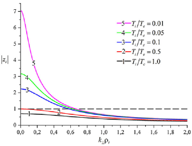In Fig.1 we present the plot of $|z_{i}|$ versus $k_{\bot}\rho_{i}$ for different values of the relation of ion to electron temperatures. It displays, that only for the ion temperature less than the electron temperature the hydrodynamic approximation $|z_{i}|\gg 1$ is valid.

Figure 1: The argument $z_{i}$ of the plasma dispersion function for the maximum growth rate (14) of the D’Angelo hydrodynamic instability versus $k_{\bot}\rho_{i}$. The dashed line corresponds to $z_{i}=1$. Below that line, Eq.(10) for the gydrodynamic growth rate is not valid.

Numerical solution to Eq.(7) is necessary because simplifying the dispersion equation (7) eliminates the ability to properly account for the ion kinetic effects. The results of the numerical solution of Eq.(7), which confirm the importance of the ion kinetic effects, are presented on Figs.2–5. Parameters considered pertinent to the conditions of SOL of Tokamaks: $\rho_{i}/L_{n}=0.002$, $v_{di}/v_{Ti}=-0.002$. Also, we assume, that $k_{x}=k_{y}=k_{\bot}/\sqrt{2}$. 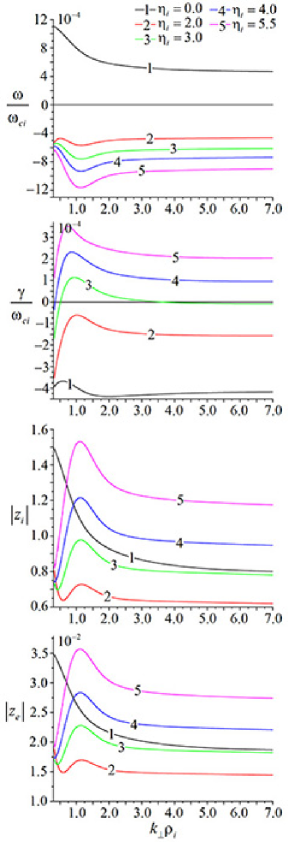In Fig.2, we present the plots of normalized frequency $\omega/\omega_{ci}$, normalized growth rate $\gamma/\omega_{ci}$, $\left|z_{i}\right|$ and $\left|z_{e}\right|$ as a function $k_{\bot}\rho_{i}$ for $V^{\prime}_{0}/\omega_{ci}=0.001$, $T_{i}/T_{e}=1.0$ and $\left(k_{z}\rho_{i}\right)^{-1}=1800$ for different values of the parameter $\eta_{i}$. The main result of Fig.2 is that the maximum growth rate is obtained in the region $k_{\bot}\rho_{i}\sim 1$, where $|z_{i}|\lesssim 1$. It is worth noting that for the case of negligible parallel-flow shear shown in Fig.2, the effect of the ion temperature gradient, $\eta_{i}$, is pronounced.

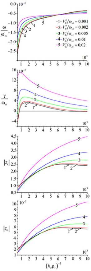
The plots of normalized frequency $\omega/\omega_{ci}$, normalized growth rate $\gamma/\omega_{ci}$, $\left|z_{i}\right|$ and $\left|z_{e}\right|$ as a function of $\left(k_{z}\rho_{i}\right)^{-1}$ for parameters $\eta_{i}=3.0$, $T_{i}/T_{e}=1.0$ and $k_{\bot}\rho_{i}=0.9$, for which the instability was predicted by Fig.2, are presented in ig.3 and Fig.4. We find that the region of the maximum growth rate corresponds to $\left(k_{z}\rho_{i}\right)^{-1}\sim 2000$. It is interesting to note, that we obtain $|z_{i}|\sim 1$ for that region.

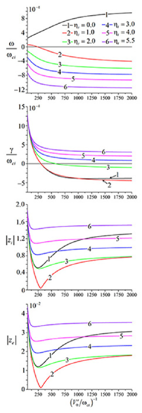
Fig.5 shows the normalized frequency $\omega/\omega_{ci}$, normalized growth rate $\gamma/\omega_{ci}$, $\left|z_{i}\right|$ and $\left|z_{e}\right|$ as a function of $\left(V^{\prime}_{0}/\omega_{ci}\right)^{-1}$ for different values of $\eta_{i}$. The parameters $k_{\bot}\rho_{i}\sim 1$, $\left(k_{z}\rho_{i}\right)^{-1}\sim 2000$ were used, at which the growth gate attains maximal value according to Figs.2–4. We find that the instability requires the presence of the ion temperature gradient $\eta_{i}$ when the value of velocity shear is small, consistent with the interpretation of Fig.2. Common to Figs.2–5, $|z_{i}|\sim 1$ in the region of maximum growth rate.

It follows from Fig.5 that at small values of $\left(V^{\prime}_{0}/\omega_{ci}\right)^{-1}$, we have $|z_{i}|>1$, independent of parameter $\eta_{i}$, and the D’Angelo instabilityChibisov develops. As $\left(V^{\prime}_{0}/\omega_{ci}\right)^{-1}$ increases, and at small values of $\eta_{i}$ parameter, the growth rate decreases and eventually becomes negative. At $\eta_{i}\geq 3$, the growth rate is positive and no longer depends on the sign or magnitude of $\left(V^{\prime}_{0}/\omega_{ci}\right)^{-1}$.

IV The kinetic, combined ion-temperature-gradient parallel-flow shear-driven (ITG-SFD) instability

Extending beyond the near-marginal-stability analysis of Rogister et al.Rogister , we consider the dispersion properties of the ITG-SFD instability for $|z_{i}|$ comparable to unity, values at which the growth rate of ITG–SFD instability is maximum. For these values of $|z_{i}|$, we take advantage of a Pade approximation for $W\left(z_{i}\right)$ in the form

$$\displaystyle W\left(z_{i}\right)\approx\frac{\sqrt{\pi}}{\sqrt{\pi}-2iz_{i}},$$ (16)

and apply it to Eq.(8). As a result, we obtain the simplest approximate dispersion equation for the kinetic ITG–SFD instability for the $|z_{i}|\lesssim 1$ domain,

$$\displaystyle z_{i}^{2}A_{0i}\eta_{i}\left|\chi_{i}\right|\left(\pi-2\right)$$

$$\displaystyle+z_{i}\left[\left(\pi-2\right)A_{0i}\left(1-\frac{k_{y}V^{\prime}_{0}}{k_{z}\omega_{ci}}\right)\right.$$

$$\displaystyle\left.-2\left(1+\frac{T_{i}}{T_{e}}-A_{0i}\right)-i\sqrt{\pi}\eta_{i}\left|\chi_{i}\right|A_{0i}\right]$$

$$\displaystyle+\pi\left|\chi_{i}\right|\left[A_{0i}\left(1-\frac{\eta_{i}}{2}\right)-\eta_{i}k_{\bot}^{2}\rho_{i}^{2}\left(A_{0i}-A_{1i}\right)\right]$$

$$\displaystyle-i\sqrt{\pi}\left(1+\frac{T_{i}}{T_{e}}-A_{0i}\frac{k_{y}V^{\prime}_{0}}{k_{z}\omega_{ci}}\right)=0.$$ (17)

Figure 2: The normalized frequency $\omega/\omega_{ci}$, normalized growth rate $\gamma/\omega_{ci}$, $\left|z_{i}\right|$ and $\left|z_{e}\right|$ versus $k_{\bot}\rho_{i}$ for $V^{\prime}_{0}/\omega_{ci}=0.001$, $T_{i}/T_{e}=1.0$ and $\left(k_{z}\rho_{i}\right)^{-1}=1800$.

Figure 3: The normalized frequency $\omega/\omega_{ci}$, normalized growth rate $\gamma/\omega_{ci}$, $\left|z_{i}\right|$ and $\left|z_{e}\right|$ versus $k_{z}\rho_{i}$ for $\eta_{i}=3.0$, $T_{i}/T_{e}=1.0$ and $k_{\bot}\rho_{i}=0.9$.

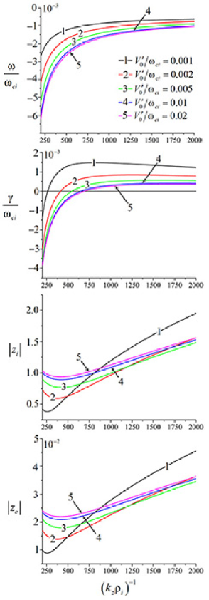
Figure 4: The normalized frequency $\omega/\omega_{ci}$, normalized growth rate $\gamma/\omega_{ci}$, $\left|z_{i}\right|$ and $\left|z_{e}\right|$ versus $(k_{z}\rho_{i})^{-1}$ between 200 and 2000, for $\eta_{i}=3.0$, $T_{i}/T_{e}=1.0$ and $k_{\bot}\rho_{i}=0.9$.

Figure 5: The normalized frequency $\omega/\omega_{ci}$, normalized growth rate $\gamma/\omega_{ci}$, $\left|z_{i}\right|$ and $\left|z_{e}\right|$ versus $\left(V^{\prime}_{0}/\omega_{ci}\right)^{-1}$ for $k_{\bot}\rho_{i}=0.9$, $T_{i}/T_{e}=1.0$ and $\left(k_{z}\rho_{i}\right)^{-1}=1800$.

This algebraic equation for $z_{i}$, in which all terms are assumed to be of the same order of value, is not more complicated analytically than the dispersion equation for the drift instabilities obtained in the opposite limit $|z_{i}|\gg 1$. It can be easily solved with solution

$$\displaystyle\frac{\omega_{i1,2}}{\sqrt{2}k_{z}v_{Ti}}=\frac{A_{0i}\pi\left(1-\frac{k_{y}V^{\prime}_{0}}{k_{z}\omega_{ci}}\right)-2\left(1+\frac{T_{i}}{T_{e}}-A_{0i}\frac{k_{y}V^{\prime}_{0}}{k_{z}\omega_{ci}}\right)}{2A_{0i}\eta_{i}\left|\chi_{i}\right|\left(\pi-2\right)}$$

$$\displaystyle\pm\sqrt{\frac{r+x}{2}},$$ (18)

$$\displaystyle\frac{\gamma_{i1,2}}{\sqrt{2}k_{z}v_{Ti}}=\frac{\sqrt{\pi}}{2\left(\pi-2\right)}\pm\sqrt{\frac{r-x}{2}},$$ (19)

where $r=\sqrt{x^{2}+y^{2}}$ and

$$\displaystyle x=\left[\frac{A_{0i}\pi\left(1-\frac{k_{y}V^{\prime}_{0}}{k_{z}\omega_{ci}}\right)-2\left(1+\frac{T_{i}}{T_{e}}-A_{0i}\frac{k_{y}V^{\prime}_{0}}{k_{z}\omega_{ci}}\right)}{2A_{0i}\eta_{i}\left|\chi_{i}\right|\left(\pi-2\right)}\right]^{2}$$

$$\displaystyle-\frac{\pi}{4\left(\pi-2\right)^{2}}$$

$$\displaystyle-\frac{\pi}{\left(\pi-2\right)}\left[\frac{2-\eta_{i}}{2\eta_{i}}-k_{\bot}^{2}\rho_{i}^{2}\left(1-\frac{A_{1i}}{A_{0i}}\right)\right],$$ (20)

$$\displaystyle y=-\frac{\sqrt{\pi}}{2\left(\pi-2\right)}\left[\frac{1}{2A_{0i}\eta_{i}\left|\chi_{i}\right|\left(\pi-2\right)}\right.$$

$$\displaystyle\times\left(A_{0i}\pi\left(1-\frac{k_{y}V^{\prime}_{0}}{k_{z}\omega_{ci}}\right)-2\left(1+\frac{T_{i}}{T_{e}}-A_{0i}\frac{k_{y}V^{\prime}_{0}}{k_{z}\omega_{ci}}\right)\right)$$

$$\displaystyle+\left.2\frac{1+\frac{T_{i}}{T_{e}}-A_{0i}\frac{k_{y}V^{\prime}_{0}}{k_{z}\omega_{ci}}}{A_{0i}\eta_{i}\left|\chi_{i}\right|}\right].$$ (21)

The ”quick” solution (18) and (19) with sign ”+” yields for the growth rate satisfactory accuracy (within five percent relative error) compared to the numerical solution of Eq.(7) presented in Fig.2, for $\eta_{i}\geq 2$ and any values of $V^{\prime}_{0}/\omega_{ci}>0$ in the region where the growth rate attains maximum value.

In the case of a plasma with homogeneous ion temperature, but with inhomogeneous density, i.e. for $\eta_{i}=0$, this instability continues to exist in the short wavelength range as the kinetic D’Angelo instabilityChibisov , which is excited due to inverse ion Landau damping. In Ref.Chibisov , the wave real frequency and the growth rate was obtained in the vicinity of the instability threshold. Eq.(17) gives for $\eta_{i}=0$ a simple expression for wave frequency and growth rate of the ion kinetic D’Angelo instability for the range over which the growth rate is maximum:

$$\displaystyle\omega=\frac{\pi A_{0i}\left|k_{y}v_{di}\right|}{\left(\pi-2\right)A_{0i}\left(\frac{k_{y}V^{\prime}_{0}}{k_{z}\omega_{ci}}-1\right)+2\left(1+\frac{T_{i}}{T_{e}}-A_{0i}\right)},$$ (22)

$$\displaystyle\gamma=\frac{\sqrt{2\pi}k_{z}v_{Ti}\left(A_{0i}\frac{k_{y}V^{\prime}_{0}}{k_{z}\omega_{ci}}-\left(1+\frac{T_{i}}{T_{e}}\right)\right)}{\left(\pi-2\right)A_{0i}\left(\frac{k_{y}V^{\prime}_{0}}{k_{z}\omega_{ci}}-1\right)+2\left(1+\frac{T_{i}}{T_{e}}-A_{0i}\right)}.$$ (23)

It follows from Eq.(23), that the instability exists for the $k_{z}\rho_{i}$ values below aa certain value

$$\displaystyle k_{z}\rho_{i}<\frac{V^{\prime}_{0}}{\omega_{ci}}\frac{A_{0i}}{1+\frac{T_{i}}{T_{e}}}k_{y}\rho_{i}.$$ (24)

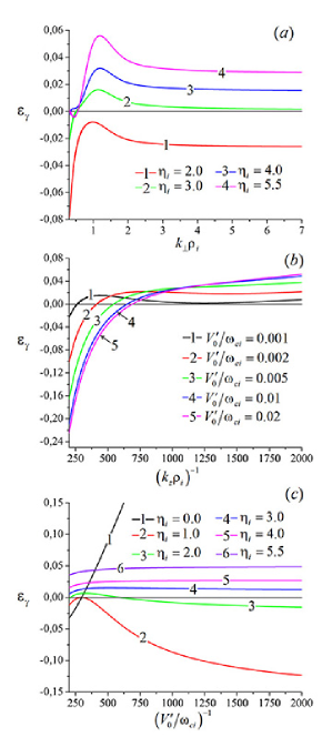
According to Fig.6, the solution (19) is valid to an accuracy of better than 10% of the relative error $\varepsilon_{\gamma}=\left(\gamma_{approx}-\gamma_{exact}\right)/\gamma_{exact}$ over the wide intervals of the pertinent parameters. In the case of the parallel-flow shear with homogeneous ion temperature Chibisov $(\eta_{i}=0)$, the relative error between the approximate solution (23) and exact numerical solution to Eq.(7) (black line on Fig. 6, case (c)) is less than 10% only for large shear, i.e. $\left(V^{\prime}_{0}/\omega_{ci}\right)^{-1}\leq 500$. The accuracy of the approximate solution (23) improves with increasing value of $\eta_{i}\neq 0$.

In Eqs.(18)–(19), it was assumed, that $\eta_{i}\neq 0$. In the different case of zero $\eta_{i}$, zero $V^{\prime}_{0}$ and $T_{i}\sim T_{e}$, Eqs.(18) and (19) predict the absence of the kinetic instability with $|z_{i}|\lesssim 1$,

$$\displaystyle\omega=\frac{\pi A_{0i}\left|k_{y}v_{di}\right|}{2\left(1+\frac{T_{i}}{T_{e}}\right)-\pi A_{0i}},$$ (25)

$$\displaystyle\frac{\gamma}{\sqrt{2}k_{z}v_{Ti}}=-\frac{\sqrt{\pi}\left(1+\frac{T_{i}}{T_{e}}\right)}{2\left(1+\frac{T_{i}}{T_{e}}\right)-\pi A_{0i}}.$$ (26)

V DISCUSSIONS AND CONCLUSIONS

In this paper, we elucidated the thermal effects of ions having inhomogeneous temperature profile on plasma stability in the presence of parallel flow shear. On the basis of the numerical solution of the general dispersion equation (7) we confirmed that the kinetic instability develops jointly with hydrodynamic D’Angelo instability due to inverse ion Landau damping and has comparable real and imaginary values of frequency at short wavelength over the interval having $k_{\perp}\rho_{i}$ of order unity.

We find that increasing the ion-temperature gradient reduces the instability threshold for the hydrodynamic D’Angelo instability and that a kinetic instability arises from the coupled, reinforcing action of parallel-flow shear and ion-temperature gradient. For the case of comparable electron and ion temperature, we illustrate analytically the transition of the D’Angelo instability to the kinetic instability as the shear parameter, the normalized wavenumber, and the ratio of density-gradient and ion-temperature-gradient scale lengths are varied.

The approximate analytical solution of the dispersion equation, which uses a simple Pade approximation (16) for the complex error function, is reported for the parameters associated with the maximum growth rate. The approximate Pade solution of the dispersion equation was compared with the numerical solution of the dispersion equation for the same plasma conditions and for numerical parameters that may be pertinent to the conditions of the scrape-off-layer in tokamaks. We find that the thermal motion of ions along the magnetic field may be important for those plasma conditions and that improvement could be derived by incorporating the parallel dynamics of ions along the magnetic field into the SOL codes. Although the dispersion equation (7) that accounted for the ion kinetic effects is the simplest one, it does not account for numerous effects such as the 3-D inhomogeneity of the toroidal magnetic field, presence of the limiters or divertors that lead to finite field-line length issues, or numerous other effects associated with the processes taking place in a tokamak or stellarator. Because of unexplored dependencies of the shear parameter on the realistic factors present in toroidal geometry, the presented plots provide only qualitative estimates for the frequency and growth rate for the D’Angelo instability in the SOL-edge layer having inhomogeneous ion temperature. For the less complicated geometry of space plasma, the estimates may prove to be more accurate. In both cases, intuition for interpreting instability and the behavior of unstable modes can be derived from the results presented here.

Figure 6: The relative error $\varepsilon_{\gamma}$ for the growth rate $\gamma$: (a) versus $k_{\bot}\rho_{i}$ for $V^{\prime}_{0}/\omega_{ci}=0.001$, $T_{i}/T_{e}=1.0$ and $k_{z}\rho_{i}=0.00055$; (b) versus $(k_{z}\rho_{i})^{-1}$ between 200 and 2000, for $\eta_{i}=5.5$, $T_{i}/T_{e}=1.0$ and $k_{\bot}\rho_{i}=0.9$; (c) versus $\left(V^{\prime}_{0}/\omega_{ci}\right)^{-1}$ for $k_{\bot}\rho_{i}=0.9$, $T_{i}/T_{e}=1.0$ and $k_{z}\rho_{i}=0.00055$.

References

(1) W. E. Amatucci, J. Geophys. Res. 104, 14481 (1999).
(2) Kintner P. M., J. Geophys. Res. 81, 5114 (1976).
(4) N. Asakura, S. Sakurai, K. Itami, O. Naito, H. Tagenaga, S.
Higashijima, Y.Koide, Y. Sakamoto, H. Kubo, and G. D. Porter, J. Nucl. Mater. 313, 820
(2003).
(5) B. LaBombard, J.E. Rice, A.E. Hubbard, J.W. Hughes, M.
Greenwald, J.Irby, Y. Lin, B. Lipschultz, E.S. Marmar, C.S. Pitchera, N. Smick, S.M. Wolfe,
S.J.Wukitch and the Alcator Group, Nucl. Fusion 44, 1047 (2004).
(6) N. Fedorczak, J.P. Gunn, Ph. Ghendrih, P. Monier-Garbet, A.
Pocheau, Journal of Nuclear Materials 390–391, 368 (2009).
(7) M.A. Pedrosa, C. Hidalgo, A. L´opez-Fraguas, M. A. Ochando,
I. Pastor, E. Calder´on and the TJ-II team, Plasma Phys. Control. Fusion 46, 221 (2004).
(18) X. Garbet, C. Fenzi, H.Capes, P.Denynck, G.Antar, Physics of
Plasmas 6,
3955 (1999).
(19) F. Schwander, G. Chiavassa, G. Ciraolo, Ph. Ghendrih, L.
Isoardi, A. Paredes, Y. Sarazin, E. Serre, P. Tamain, Journal of Nuclear Materials 415 S601
(2011)
(20) C. Fenzi, P. Devynck, A. Truc, X. Garbet, H. Capes, C. Laviron, G. Antar, F.
Gervais, P. Hennequin, A. Quéméneur, Plasma Phys. Contr. Fusion 41, 1043 (1999)
(21) N. D’Angelo, Phys. Fluids 8, 1748 (1965).
(22) S. Migliuolo, J.Geophys.Res. 93, 867 (1988).
(23) A. Rogister, R. Singh, P.K. Kaw, Physics of Plasmas 11, 2106 (2004).
(24) V.Gavrishchaka, S.Ganguli, and G.Ganguli, Phys.Rev.Lett. 80, 728
(1998).
(25) V.Gavrishchaka , S.Ganguli, and G.Ganguli, J. Geophys. Res.