Convex Relaxation of Optimal Power Flow
Part II: Exactness

Abstract

This tutorial summarizes recent advances in the convex relaxation of the optimal power flow (OPF) problem, focusing on structural properties rather than algorithms. Part I presents two power flow models, formulates OPF and their relaxations in each model, and proves equivalence relations among them. Part II presents sufficient conditions under which the convex relaxations are exact.

May 1, 2014

Acknowledgment. We thank the support of NSF through NetSE CNS 0911041, ARPA-E through GENI DE-AR0000226, Southern California Edison, the National Science Council of Taiwan through NSC 103-3113-P-008-001, the Los Alamos National Lab (DoE), and Caltech’s Resnick Institute.

I Introduction

The optimal power flow (OPF) problem is fundamental in power systems as it underlies many applications such as economic dispatch, unit commitment, state estimation, stability and reliability assessment, volt/var control, demand response, etc. OPF seeks to optimize a certain objective function, such as power loss, generation cost and/or user utilities, subject to Kirchhoff’s laws as well as capacity, stability and security constraints on the voltages and power flows. There has been a great deal of research on OPF since Carpentier’s first formulation in 1962 [1]. Recent surveys can be found in, e.g., [2, 3, 4, 5, 6, 7, 8, 9, 10, 11, 12, 13].

OPF is generally nonconvex and NP-hard, and a large number of optimization algorithms and relaxations have been proposed. To the best of our knowledge solving OPF through semidefinite relaxation is first proposed in [14] as a second-order cone program (SOCP) for radial (tree) networks and in [15] as a semidefinite program (SDP) for general networks in a bus injection model. It is first proposed in [16, 17] as an SOCP for radial networks in the branch flow model of [18, 19]. While these convex relaxations have been illustrated numerically in [14] and [15], whether or when they will turn out to be exact is first studied in [20]. Exploiting graph sparsity to simplify the SDP relaxation of OPF is first proposed in [21, 22] and analyzed in [23, 24].

Solving OPF through convex relaxation offers several advantages, as discussed in Part I of this tutorial [25, Section I]. In particular it provides the ability to check if a solution is globally optimal. If it is not, the solution provides a lower bound on the minimum cost and hence a bound on how far any feasible solution is from optimality. Unlike approximations, if a relaxed problem is infeasible, it is a certificate that the original OPF is infeasible.

This tutorial presents main results on convex relaxations of OPF developed in the last few years. In Part I [25], we present the bus injection model (BIM) and the branch flow model (BFM), formulate OPF within each model, and prove their equivalence. The complexity of OPF formulated here lies in the quadratic nature of power flows, i.e., the nonconvex quadratic constraints on the feasible set of OPF. We characterize these feasible sets and design convex supersets that lead to three different convex relaxations based on semidefinite programming (SDP), chordal extension, and second-order cone programming (SOCP). When a convex relaxation is exact, an optimal solution of the original nonconvex OPF can be recovered from every optimal solution of the relaxation. In Part II we summarize main sufficient conditions that guarantee the exactness of these relaxations.

Network topology turns out to play a critical role in determining whether a relaxation is exact. In Section II we review the definitions of OPF and their convex relaxations developed in [25]. We also define the notion of exactness adopted in this paper. In Section III we present three types of sufficient conditions for these relaxations to be exact for radial networks. These conditions are generally not necessary and they have implications on allowable power injections, voltage magnitudes, or voltage angles:

1. Power injections: These conditions require that not both constraints on real and reactive power injections be binding at both ends of a line.

2. Voltages magnitudes: These conditions require that the upper bounds on voltage magnitudes not be binding. They can be enforced through affine constraints on power injections.

3. Voltage angles: These conditions require that the voltage angles across each line be sufficiently close. This is needed also for stability reasons.

These conditions and their references are summarized in Tables II and II.

type	condition	model	reference	remark
A	power injections	BIM, BFM	[26, 27, 28, 29, 30]
			[31, 16, 17]
B	voltage magnitudes	BFM	[32, 33, 34, 35]	allows general injection region
C	voltage angles	BIM	[36, 37]	makes use of branch power flows

TABLE I: Sufficient conditions for radial (tree) networks.

network	condition	reference	remark
with phase shifters	type A, B, C	[17, Part II], [38]	equivalent to radial networks
direct current	type A	[17, Part I], [20, 39]	assumes nonnegative voltages
	type B	[40, 41]	assumes nonnegative voltages

TABLE II: Sufficient conditions for mesh networks

Some of these sufficient conditions are proved using BIM and others using BFM. Since these two models are equivalent (in the sense that there is a linear bijection between their solution sets [24, 25]), these sufficient conditions apply to both models. The proofs of these conditions typically do not require that the cost function be convex (they focus on the feasible sets and usually only need the cost function to be monotonic). Convexity is required however for efficient computation. Moreover it is proved in [35] using BFM that when the cost function is convex then exactness of the SOCP relaxation implies uniqueness of the optimal solution for radial networks. Hence the equivalence of BIM and BFM implies that any of the three types of sufficient conditions guarantees that, for a radial network with a convex cost function, there is a unique optimal solution and it can be computed by solving an SOCP. Since the SDP and chordal relaxations are equivalent to the SOCP relaxation for radial networks [24, 25], these results apply to all three types of relaxations. Empirical evidences suggest some of these conditions are likely satisfied in practice. This is important as most power distribution systems are radial.

These conditions are insufficient for general mesh networks because they cannot guarantee that an optimal solution of a relaxation satisfies the cycle condition discussed in [25]. In Section IV we show that these conditions are however sufficient for mesh networks that have tunable phase shifters at strategic locations. The phase shifters effectively make a mesh network behave like a radial network as far as convex relaxation is concerned. The result can help determine if a network with a given set of phase shifters can be convexified and, if not, where additional phase shifters are needed for convexification. These conditions are also sufficient for direct current (dc) mesh networks where all variables are in the real rather than complex domain. Counterexamples are known where SDP relaxation is not exact, especially for AC mesh networks without tunable phase shifters [42, 43]. We discuss three recent approaches for global optimization of OPF when the semidefinite relaxations discussed in this tutorial fail.

We conclude in Section V. This extended version differs from the journal version only in the addition of Appendix VI that proves all main results covered in this tutorial. Even though all proofs can be found in their original papers, we provide proofs here because (i) it is convenient to have all proofs in one place and in a uniform notation, and (ii) some of the formulations and presentations here are slightly different from those in the original papers.

II OPF and its relaxations

We use the notations and definitions from Part I of this paper. In this section we summarize the OPF problems and their relaxations developed there; see [25] for details.

We adopt in this paper a strong sense of “exactness” where we require the optimal solution set of the OPF problem and that of its relaxation be equivalent. This implies that an optimal solution of the nonconvex OPF problem can be recovered from every optimal solution of its relaxation. This is important because it ensures any algorithm that solves an exact relaxation always produces a globally optimal solution to the OPF problem. Indeed interior point methods for solving SDPs tend to produce a solution matrix with a maximum rank [44], so can miss a rank-1 solution if the relaxation has non-rank-1 solutions as well. It can be difficult to recover an optimal solution of OPF from such a non-rank-1 solution, and our definition of exactness avoids this complication. See Section II-C for detailed justifications.

II-A Bus injection model

The BIM adopts an undirected graph $G$ and can be formulated in terms of just the complex voltage vector $V\in\mathbb{C}^{n+1}$. The feasible set is described by the following constraints:

$$\quad\underline{s}_{j}\ \ \leq\sum_{k:(j,k)\in E}y_{jk}^{H}\,V_{j}(V_{j}^{H}-V_{k}^{H})\ \ \leq\ \ \overline{s}_{j},\qquad j\in N^{+}$$ (1a)

$$\qquad\qquad\underline{v}_{j}\ \leq\ \ |V_{j}|^{2}\ \ \leq\ \overline{v}_{j},\qquad\qquad j\in N^{+}$$ (1b)

where $\underline{s}_{j},\overline{s}_{j},\underline{v}_{j},\overline{v}_{j}$, possibly $\pm\infty\pm\textbf{i}\infty$, are given bounds on power injections and voltage magnitudes. Note that the vector $V$ includes $V_{0}$ which is assumed given ($\underline{v}_{0}=\overline{v}_{0}$ and $\angle V_{0}=0^{\circ}$) unless otherwise specified. The problem of interest is:
OPF:

$$\underset{V\in\mathbb{C}^{n+1}}{\text{min}}\ C(V)\ V\text{ satisfies }\eqref{eq:bimopf}$$ subject to (2)

For relaxations consider the partial matrix $W_{G}$ defined on the network graph $G$ that satisfies

$$\underline{s}_{j}\ \leq\!\!\sum_{k:(j,k)\in E}\!\!y_{jk}^{H}\,\left([W_{G}]_{jj}-[W_{G}]_{jk}\right)\leq\ \overline{s}_{j},\qquad j\in N^{+}$$ (3a)

$$\underline{v}_{j}\ \leq\ [W_{G}]_{jj}\ \leq\ \overline{v}_{j},\qquad\qquad j\in N^{+}$$ (3b)

We say that $W_{G}$ satisfies the cycle condition if for every cycle $c$ in $G$

$$\sum_{(j,k)\in c}\ \angle[W_{G}]_{jk} = 0\ \ \mod 2\pi$$ (4)

We assume the cost function $C$ depends on $V$ only through $VV^{H}$ and use the same symbol $C$ to denote the cost in terms of a full or partial matrix. Moreover we assume $C$ depends on the matrix only through the submatrix $W_{G}$ defined on the network graph $G$. See [25, Section IV] for more details including the definitions of $W_{c(G)}\succeq 0$ and $W_{G}(j,k)\succeq 0$. Define the convex relaxations:
OPF-sdp:

$$\underset{W\in\mathbb{S}^{n+1}}{\text{min}}\ C(W_{G})\ W_{G}\text{ satisfies }\eqref{eq:opfW},\ W\succeq 0$$ subject to (5)

OPF-ch:

$$\underset{W_{c(G)}}{\text{min}}\ C(W_{G})\ W_{G}\text{ satisfies }\eqref{eq:opfW},\ W_{c(G)}\succeq 0$$ subject to (6)

OPF-socp:

$$\ \ \underset{W_{G}}{\text{min}}\ C(W_{G})\ W_{G}\text{ satisfies }\eqref{eq:opfW},\ W_{G}(j,k)\succeq 0,\ (j,k)\in E$$ subject to (7)

For BIM, we say that OPF-sdp (5) is exact if every optimal solution $W^{\text{sdp}}$ of OPF-sdp is psd rank-1; OPF-ch (6) is exact if every optimal solution $W_{c(G)}^{\text{ch}}$ of OPF-ch is psd rank-1 (i.e., the principal submatrices $W_{c(G)}^{\text{ch}}(q)$ of $W_{c(G)}^{\text{ch}}$ are psd rank-1 for all maximal cliques $q$ of the chordal extension $c(G)$ of graph $G$); OPF-socp (7) is exact if every optimal solution $W_{G}^{\text{socp}}$ of OPF-socp is $2\times 2$ psd rank-1 and satisfies the cycle condition (4). To recover an optimal solution $V^{\text{opt}}$ of OPF (2) from $W^{\text{sdp}}$ or $W_{c(G)}^{\text{ch}}$ or $W_{G}^{\text{socp}}$, see [25, Section IV-D].

II-B Branch flow model

The BFM adopts a directed graph $\tilde{G}$ and is defined by the following set of equations:

$$\!\!\!\!\sum_{k:j\rightarrow k}\!\!\!S_{jk} \!\!=\!\! \!\!\!\!\sum_{i:i\rightarrow j}\!\!\left(S_{ij}-z_{ij}|I_{ij}|^{2}\right)+s_{j},\qquad j\in N^{+}$$ (8a)

$$\!\!\!\!I_{jk} \!\!=\!\! y_{jk}(V_{j}-V_{k}),\qquad\qquad\,j\rightarrow k\in\tilde{E}$$ (8b)

$$\!\!\!\!S_{jk} \!\!=\!\! V_{j}\,I_{jk}^{H},\qquad\qquad\qquad\ \ \,j\rightarrow k\in\tilde{E}$$ (8c)

Denote the variables in BFM (8) by $\tilde{x}:=(S,I,V,s)\in\mathbb{C}^{2(m+n+1)}$. Note that the vectors $V$ and $s$ include $V_{0}$ (given) and $s_{0}$ respectively. Recall from [25] the variables $x:=(S,\ell,v,s)\in\mathbb{R}^{3(m+n+1)}$ that is related to $\tilde{x}$ by the mapping $x=h(\tilde{x})$ with $\ell_{jk}:=|I_{jk}|^{2}$ and $v_{j}:=|V_{j}|^{2}$. The operational constraints are:

$$\underline{v}_{j}\ \leq v_{j} \leq\ \overline{v}_{j},\qquad j\in N^{+}$$ (9a)

$$\underline{s}_{j}\ \leq s_{j} \leq\ \overline{s}_{j},\qquad j\in N^{+}$$ (9b)

We assume the cost function depends on $\tilde{x}$ only through $x=h(\tilde{x})$. Then the problem in BFM is:
OPF:

$$\underset{\tilde{x}}{\text{min}}\ \ C(x) \tilde{x}\text{ satisfies }\eqref{eq:bfm},\eqref{eq:bfmopf}$$ subject to (10)

For SOCP relaxation consider:

$$\!\!\!\!\!\sum_{k:j\rightarrow k}S_{jk} \!\!\!=\!\!\! \!\!\sum_{i:i\rightarrow j}\left(S_{ij}-z_{ij}\ell_{ij}\right)+s_{j},\qquad\qquad\ \ \ j\in N^{+}$$ (11a)

$$\!\!\!\!\!v_{j}-v_{k} \!\!\!=\!\!\! 2\,\text{Re}\left(z_{jk}^{H}S_{jk}\right)-|z_{jk}|^{2}\ell_{jk},\qquad j\rightarrow k\in\tilde{E}$$ (11b)

$$\!\!\!\!\!v_{j}\ell_{jk} \!\!\!\geq\!\!\! |S_{jk}|^{2},\qquad\qquad\qquad\qquad\quad\ \,j\rightarrow k\in\tilde{E}$$ (11c)

We say that $x$ satisfies the cycle condition if

$$\!\!\!\!\!\!\exists\theta\in\mathbb{R}^{n} B\theta=\beta(x)\mod 2\pi$$ such that (12)

where $B$ is the $m\times n$ reduced incidence matrix and, given $x:=(S,\ell,v,s)$, $\beta_{jk}(x):=\angle(v_{j}-z_{jk}^{H}S_{jk})$ can be interpreted as the voltage angle difference across line $j\rightarrow k$ implied by $x$ (See [25, Section V]). The SOCP relaxation in BFM is
OPF-socp:

$$\underset{x}{\text{min}}\ \ C(x) x\text{ satisfies }\eqref{eq:mdf},\eqref{eq:bfmopf}$$ subject to (13)

For BFM, OPF-socp (13) in BFM is exact if every optimal solution $x^{\text{socp}}$ attains equality in (11c) and satisfies the cycle condition (12). See [25, Section V-A] for how to recover an optimal solution $\tilde{x}^{\text{opt}}$ of OPF (10) from any optimal solution $x^{\text{socp}}$ of its SOCP relaxation.

II-C Exactness

The definition of exactness adopted in this paper is more stringent than needed. Consider SOCP relaxation in BIM as an illustration (the same applies to the other relaxations in BIM and BFM). For any sets $A$ and $B$, we say that $A$ is equivalent to $B$, denoted by $A\equiv B$, if there is a bijection between these two sets. Let $\mathbb{M}(A)$ denote the set of minimizers when a certain function is minimized over $A$.

Let $\mathbb{V}$ and $\mathbb{W}_{G}^{+}$ denote the feasible sets of OPF (2) and OPF-socp (7) respectively:

$$\mathbb{V} \!\!\!\!:=\!\!\!\! \{V\in\mathbb{C}^{n+1}\ |\ V\text{ satisfies }\eqref{eq:bimopf}\}$$

$$\mathbb{W}_{G}^{+} \!\!\!\!:=\!\!\!\! \{W_{G}\ |\ W_{G}\text{ satisfies }\eqref{eq:opfW},\ W_{G}(j,k)\succeq 0,\ (j,k)\in E\}$$

Consider the following subset of $\mathbb{W}_{G}^{+}$:

$$\mathbb{W}_{G} := \{W_{G}\ |\ W_{G}\text{ satisfies }\eqref{eq:opfW},\eqref{eq:cyclecond.2},\ W_{G}(j,k)\succeq 0,\,\text{rank}\,W_{G}(j,k)=1,\ (j,k)\in E\}$$

Our definition of exact SOCP relaxation is that $\mathbb{M}(\mathbb{W}_{G}^{+})\subseteq\mathbb{W}_{G}$. In particular, all optimal solutions of OPF-socp must be $2\times 2$ psd rank-1 and satisfy the cycle condition (4). Since $\mathbb{W}_{G}\equiv\mathbb{V}$ (see [25]), exactness requires that the set of optimal solutions of OPF-socp (7) be equivalent to that of OPF (2), i.e., $\mathbb{M}(\mathbb{W}_{G}^{+})=\mathbb{M}(\mathbb{W}_{G})\equiv\mathbb{M}(\mathbb{V})$.

If $\mathbb{M}(\mathbb{W}_{G}^{+})\supsetneq\mathbb{M}(\mathbb{W}_{G})\equiv\mathbb{M}(\mathbb{V})$ then OPF-socp (7) is not exact according to our definition. Even in this case, however, every sufficient condition in this paper guarantees that an optimal solution of OPF can be easily recovered from an optimal solution of the relaxation that is outside $\mathbb{W}_{G}$. The difference between $\mathbb{M}(\mathbb{W}_{G}^{+})=\mathbb{M}(\mathbb{W}_{G})$ and $\mathbb{M}(\mathbb{W}_{G}^{+})\supsetneq\mathbb{M}(\mathbb{W}_{G})$ is often minor, depending on the objective function; see Remarks 1 and 2 and comments after Theorems 5 and 8 in Section III. Hence we adopt the more stringent definition of exactness for simplicity.

III Radial networks

In this section we summarize the three types of sufficient conditions listed in Table II for semidefinite relaxations of OPF to be exact for radial (tree) networks. These results are important as most distribution systems are radial.

For radial networks, if SOCP relaxation is exact then SDP and chordal relaxations are also exact (see [25, Theorems 5, 9]). We hence focus in this section on the exactness of OPF-socp in both BIM and BFM. Since the cycle conditions (4) and (12) are vacuous for radial networks, OPF-socp (7) is exact if all of its optimal solutions are $2\times 2$ rank-1 and OPF-socp (13) is exact if all of its optimal solutions attain equalities in (11c). We will freely use either BIM or BFM in discussing these results. To avoid triviality we make the following assumption throughout the paper:

1. The voltage lower bounds satisfy $\underline{v}_{j}>0$, $j\in N^{+}$. The original problems OPF (2) and (10) are feasible.

III-A Linear separability

We will first present a general result on the exactness of the SOCP relaxation of general QCQP and then apply it to OPF. This result is first formulated and proved using a duality argument in [27], generalizing the result of [26]. It is proved using a simpler argument in [31].

Fix an undirected graph $G=(N^{+},E)$ where $N^{+}:=\{0,1,\dots,n\}$ and $E\subseteq N^{+}\times N^{+}$. Fix Hermitian matrices $C_{l}\in\mathbb{S}^{n+1}$, $l=0,\dots,L$, defined on $G$, i.e., $[C_{l}]_{jk}=0$ if $(j,k)\not\in E$. Consider QCQP:

$$\underset{x\in\mathbb{C}^{n+1}}{\text{min}} \!\!\!\!x^{{H}}C_{0}x$$ (14a)

subject to $$\!\!\!\!x^{{H}}C_{l}x\leq b_{l},\ \ l=1,\dots,L$$ (14b)

where $C_{0},C_{l}\in\mathbb{C}^{(n+1)\times(n+1)}$, $b_{l}\in\mathbb{R}$, $l=1,\dots,L$, and its SOCP relaxation where the optimization variable ranges over Hermitian partial matrices $W_{G}$:

$$\underset{W_{G}}{\text{min}} \!\!\!\!\!\text{tr }C_{0}W_{G}$$ (15a)

subject to $$\!\!\!\!\!\text{tr }C_{l}W_{G}\leq b_{l},\ \ l=1,\dots,L$$ (15c)

$$\!\!\!\!\!W_{G}(j,k)\succeq 0,\ \ (j,k)\in E$$

The following result is proved in [27, 31]. It can be regarded as an extension of [45] on the SOCP relaxation of QCQP from the real domain to the complex domain. Consider:

1. The cost matrix $C_{0}$ is positive definite.

2. For each link $(j,k)\in E$ there exists an $\alpha_{jk}$ such that $\angle\left[C_{l}\right]_{jk}\in[\alpha_{ij},\alpha_{ij}+\pi]$ for all $l=0,\dots,L$.

Let $C^{\text{opt}}$ and $C^{\text{socp}}$ denote the optimal values of QCQP (14) and SOCP (15) respectively.

Theorem 1

Suppose $G$ is a tree and A2 holds. Then $C^{\text{opt}}=C^{\text{socp}}$ and an optimal solution of QCQP (14) can be recovered from every optimal solution of SOCP (15).

Remark 1

The proof of Theorem 1 prescribes a simple procedure to recover an optimal solution of QCQP (14) from any optimal solution of its SOCP relaxation (15). The construction does not need the optimal solution of SOCP (15) to be $2\times 2$ rank-1. Hence the SOCP relaxation may not be exact according to our definition of exactness, i.e., some optimal solutions of (15) may be $2\times 2$ psd but not $2\times 2$ rank-1. If the objective function is strictly convex however then the optimal solution sets of QCQP (14) and SOCP (15) are indeed equivalent.

Corollary 2

Suppose $G$ is a tree and A1–A2 hold. Then SOCP (15) is exact.

We now apply Theorem 1 to our OPF problem. Recall that OPF (2) in BIM can be written as a standard form QCQP [27]:

$$\!\!\!\!\!\!\!\!\!\!\!\!\!\min_{x\in\mathbb{C}^{n}} \!\!\!\!V^{H}C_{0}V$$

s.t. $$\!\!\!\!V^{H}\Phi_{j}V\leq\overline{p}_{j},\ V^{H}(-\Phi_{j})V\leq-\underline{p}_{j}$$

$$\!\!\!\!V^{H}\Psi_{j}V\leq\overline{q}_{j},\ V^{H}(-\Psi_{j})V\leq-\underline{q}_{j}$$

$$\!\!\!\!V^{H}J_{j}V\leq-\overline{v}_{j},\ V^{H}(-J_{j})V\leq-\underline{v}_{j}$$

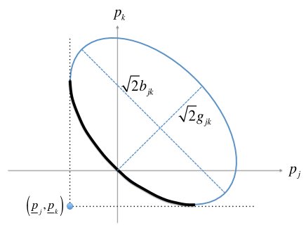
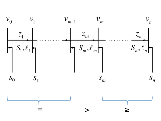
for some Hermitian matrices $C_{0},\Phi_{j},\Psi_{j},J_{j}$ where $j\in N^{+}$. A2 depends only on the off-diagonal entries of $C_{0}$, $\Phi_{j}$, $\Psi_{j}$ ($J_{j}$ are diagonal matrices). It implies a simple pattern on the power injection constraints (16)–(16). Let $y_{jk}=g_{jk}-\textbf{i}b_{jk}$ with $g_{jk}>0,b_{jk}>0$. Then we have (from [27]):

$$[\Phi_{k}]_{ij} \!\!\!\!=\!\!\!\! \begin{cases}\frac{1}{2}Y_{ij}\,=\,-\frac{1}{2}(g_{ij}-\textbf{i}b_{ij})&\text{ if }k=i\\ \frac{1}{2}{Y}_{ij}^{H}\,=\,-\frac{1}{2}(g_{ij}+\textbf{i}b_{ij})&\text{ if }k=j\\ 0&\text{ if }k\not\in\{i,j\}\end{cases}$$

$$[\Psi_{k}]_{ij} \!\!\!\!=\!\!\!\! \begin{cases}\frac{-1}{2\textbf{i}}Y_{ij}\,=\,-\frac{1}{2}(b_{ij}+\textbf{i}g_{ij})&\text{if }k=i\\ \frac{1}{2\textbf{i}}{Y}_{ij}^{H}\,=\,-\frac{1}{2}(b_{ij}-\textbf{i}g_{ij})&\text{if }k=j\\ 0&\text{if }k\not\in\{i,j\}\end{cases}$$

Hence for each line $(j,k)\in E$ the relevant angles for A2 are those of $[C_{0}]_{jk}$ and

$$\left[\Phi_{j}\right]_{jk} = -\frac{1}{2}(g_{jk}-\textbf{i}b_{jk})$$

$$[\Phi_{k}]_{jk} = -\frac{1}{2}(g_{jk}+\textbf{i}b_{jk})$$

$$[\Psi_{j}]_{jk} = -\frac{1}{2}(b_{jk}+\textbf{i}g_{jk})$$

$$[\Psi_{k}]_{jk} = -\frac{1}{2}(b_{jk}-\textbf{i}g_{jk})$$

as well as the angles of $-[\Phi_{j}]_{jk},-[\Phi_{k}]_{jk}$ and $-[\Psi_{j}]_{jk},-[\Psi_{k}]_{jk}$. These quantities are shown in Figure 1 with their magnitudes normalized to a common value and explained in the caption of the figure.

Figure 1: Condition A2’ on a line $(j,k)\in E$. The quantities $([\Phi_{j}]_{jk},[\Phi_{k}]_{jk},[\Psi_{j}]_{jk},[\Psi_{k}]_{jk})$ on the left-half plane correspond to finite upper bounds on $(p_{j},p_{k},q_{j},q_{k})$ in (16)–(16); $(-[\Phi_{j}]_{jk},-[\Phi_{k}]_{jk},-[\Psi_{j}]_{jk},-[\Psi_{k}]_{jk})$ on the right-half plane correspond to finite lower bounds on $(p_{j},p_{k},q_{j},q_{k})$. A2’ is satisfied if there is a line through the origin, specified by the angle $\alpha_{jk}$, so that the quantities corresponding to finite upper or lower bounds on $(p_{j},p_{k},q_{j},q_{k})$ lie on one side of the line, possibly on the line itself. The load over-satisfaction condition in [26, 30] corresponds to the Im-axis that excludes all quantities on the right-half plane. The sufficient condition in [29, Theorem 2] corresponds to the red line in the figure that allows a finite lower bound on the real power at one end of the line, i.e., $p_{j}$ or $p_{k}$ but not both, and no finite lower bounds on reactive powers $q_{j}$ and $q_{k}$.

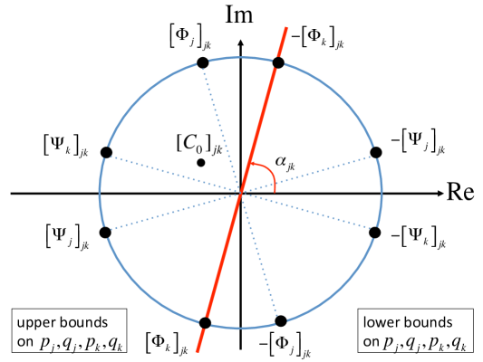
Condition A2 applied to OPF (16) takes the following form (see Figure 1):

1. For each link $(j,k)\in E$ there is a line in the complex plane through the origin such that $\left[C_{0}\right]_{jk}$ as well as those $\pm[\Phi_{i}]_{jk}$ and $\pm[\Psi_{i}]_{jk}$ corresponding to finite lower or upper bounds on $(p_{i},q_{i})$, for $i=j,k$, are all on one side of the line, possibly on the line itself.

Let $C^{\text{opt}}$ and $C^{\text{socp}}$ denote the optimal values of OPF (2) and OPF-socp (7) respectively.

Corollary 3

Suppose $G$ is a tree and A2’ holds.

1. $C^{\text{opt}}=C^{\text{socp}}$. Moreover an optimal solution $V^{\text{opt}}$ of OPF (2) can be recovered from every optimal solution $W_{G}^{\text{socp}}$ of OPF-socp (7).

2. If, in addition, A1 holds then OPF-socp (7) is exact.

It is clear from Figure 1 that condition A2’ cannot be satisfied if there is a line where both the real and reactive power injections at both ends are both lower and upper bounded (8 combinations as shown in the figure). A2’ requires that some of them be unconstrained even though in practice they are always bounded. It should be interpreted as requiring that the optimal solutions obtained by ignoring these bounds turn out to satisfy these bounds. This is generally different from solving the optimization with these constraints but requiring that they be inactive (strictly within these bounds) at optimality, unless the cost function is strictly convex. The result proved in [27] also includes constraints on real branch power flows and line losses. Corollary 3 includes several sufficient conditions in the literature for exact relaxation as special cases; see the caption of Figure 1.

Corollary 3 also implies a result first proved in [16], using a different technique, that SOCP relaxation is exact in BFM for radial networks when there are no lower bounds on power injections $s_{j}$. The argument in [16] is generalized in [17, Part I] to allow convex objective functions, shunt elements, and line limits in terms of upper bounds on $\ell_{jk}$. Assume

1. The cost function $C(x)$ is convex, strictly increasing in $\ell$, nondecreasing in $s=(p,q)$, and independent of branch flows $S=(P,Q)$.

2. For $j\in N^{+}$, $\underline{s}_{j}=-\infty-\textbf{i}\infty$.

Popular cost functions in the literature include active power loss over the network or active power generations, both of which satisfy A3. The next result is proved in [16, 17].

Theorem 4

Suppose $\tilde{G}$ is a tree and A3–A4 hold. Then OPF-socp (13) is exact.

Remark 2

If the cost function $C(x)$ in A3 is only nondecreasing, rather than strictly increasing, in $\ell$, then A3–A4 still guarantee that all optimal solutions of OPF (10) are (i.e., can be mapped to) optimal solutions of OPF-socp (13), but OPF-socp may have an optimal solution that maintains strict inequalities in (11c) and hence is infeasible for OPF. Even though OPF-socp is not exact in this case, the proof of Theorem 4 constructs from it an optimal solution of OPF (See the arXiv version of this paper).

III-B Voltage upper bounds

While type A conditions (A2’ and A4 in the last subsection) require that some power injection constraints not be binding, type B conditions require non-binding voltage upper bounds. They are proved in [32, 33, 34, 35] using BFM.

For radial networks the model originally proposed in [18, 19], which is (11) with the inequalities in (11c) replaced by equalities, is exact. This is because the cycle condition (12) is always satisfied as the reduced incidence matrix $B$ is $n\times n$ and invertible for radial networks. Following [35] we adopt the graph orientation where every link points towards node 0. Then (11) for a radial network reduces to:

$$\!\!\!\!\!\!\!\!\!{S}_{jk} \!\!\!\!=\!\!\!\! \!\!\sum_{i:i\rightarrow j}\!\!\left({S}_{ij}-z_{ij}\ell_{ij}\right)+s_{j},\qquad\qquad\ \ \ \,j\in N^{+}$$ (17a)

$$\!\!\!\!\!\!\!\!\!v_{j}-v_{k} \!\!\!\!=\!\!\!\! 2\,\text{Re}\left(z_{jk}^{H}S_{jk}\right)\!-|z_{jk}|^{2}\ell_{jk},\qquad j\rightarrow k\in\tilde{E}$$ (17b)

$$\!\!\!\!\!\!\!\!\!v_{j}\ell_{jk} \!\!\!\!\geq\!\!\!\! |S_{jk}|^{2},\qquad\qquad\qquad\qquad\quad\ j\rightarrow k\in\tilde{E}$$ (17c)

where $v_{0}$ is given and in (17a), $k$ denotes the node on the unique path from node $j$ to node 0. The boundary condition is: $S_{jk}:=0$ when $j=0$ in (17a) and $S_{ij}=0$, $\ell_{ij}=0$ when $j$ is a leaf node.

As before the voltage magnitudes must satisfy:

$$\underline{v}_{j}\ \leq v_{j} \leq\ \overline{v}_{j},\qquad j\in N$$ (18a)

We allow more general constraints on the power injections: for $$j\in N s_{j} \mathbb{S}_{j}$$, can be in an arbitrary set that is bounded above:

$$s_{j}\ \in\ \mathbb{S}_{j} \subseteq \{s_{j}\in\mathbb{C}\,|\,s_{j}\leq\overline{s}_{j}\},\qquad j\in N$$ (18b)

for some given $\overline{s}_{j}$, $j\in N$. Then the SOCP relaxation is
OPF-socp:

$$\underset{x}{\text{min}}\ \ C(x) \eqref{eq:gdf},\eqref{eq:cnstrs}\qquad\quad$$ subject to (19)

As defined in Section II-C, OPF-socp (19) is exact if every optimal solution $x^{\text{socp}}$ attains equality in (17c). In that case an optimal solution of BFM (10) can be uniquely recovered from $x^{\text{socp}}$.

We make two comments on the constraint sets $\mathbb{S}_{j}$ in (18b). First $\mathbb{S}_{j}$ need not be convex nor even connected for convex relaxations to be exact. They (only) need to be convex to be efficiently computable. Second such a general constraint on $s$ is useful in many applications. It includes the case where $s_{j}$ are subject to simple box constraints, but also allows constraints of the form $|s_{j}|^{2}\leq a$, $|\angle s_{j}|\leq\phi_{j}$ that is useful for volt/var control [46], or $q_{j}\in\{0,a\}$ for capacitor configurations.

Geometric insight. To motivate our sufficient condition, we first explain a simple geometric intuition using a two-bus network on why relaxing voltage upper bounds guarantees exact SOCP relaxation. Consider bus 0 and bus 1 connected by a line with impedance $z:=r+\textbf{i}x$. Suppose without loss of generality that $v_{0}=1$ pu. Eliminating $S_{01}=s_{0}$ from (17), the model reduces to (dropping the subscript on $\ell_{01}$):

$$p_{0}-r\ell\ =\ -p_{1},\ \ \ q_{0}-x\ell\ =\ -q_{1},\ \ \ p_{0}^{2}+q_{0}^{2}\ =\ \ell$$ (20)

and

$$v_{1}-v_{0} = 2(rp_{0}+xq_{0})-|z|^{2}\ell$$ (21)

Suppose $s_{1}$ is given (e.g., a constant power load). Then the variables are $(\ell,v_{1},p_{0},q_{0})$ and the feasible set consists of solutions of (20) and (21) subject to additional constraints on $(\ell,v_{1},p_{0},q_{0})$.

Figure 2: Feasible set of OPF for a two-bus network without any constraint. It consists of the (two) points of intersection of the line with the convex surface (without the interior), and hence is nonconvex. SOCP relaxation includes the interior of the convex surface and enlarges the feasible set to the line segment joining these two points. If the cost function $C$ is increasing in $\ell$ or $(p_{0},q_{0})$ then the optimal point over the SOCP feasible set (line segment) is the lower feasible point $c$, and hence the relaxation is exact. No constraint on $\ell$ or $(p_{0},q_{0})$ will destroy exactness as long as the resulting feasible set contains $c$.

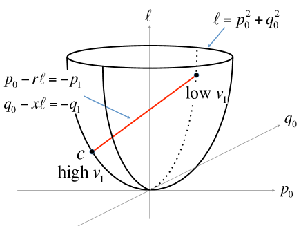
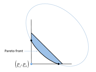
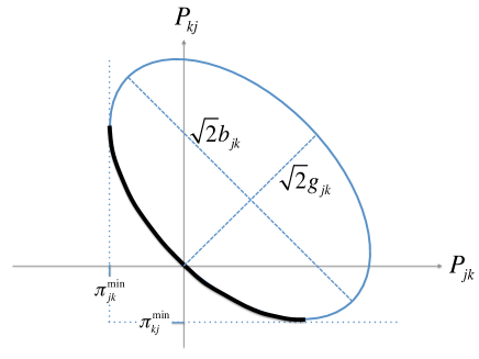
The case without any constraint is instructive and shown in Figure 2. The point $c$ in the figure corresponds to a power flow solution with a large $v_{1}$ (normal operation) whereas the other intersection corresponds to a solution with a small $v_{1}$ (fault condition). As explained in the caption, SOCP relaxation is exact if there is no voltage constraint and as long as constraints on $(\ell,p_{0},q_{0})$ does not remove the high-voltage (normal) power flow solution $c$. Only when the system is stressed to a point where the high-voltage solution becomes infeasible will relaxation lose exactness. This agrees with conventional wisdom that power systems under normal operations are well behaved.

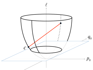
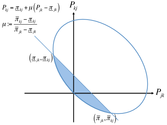
Consider now the voltage constraint $\underline{v}_{1}\leq v_{1}\leq\overline{v}_{1}$. Substituting (20) into (21) we obtain

$$v_{1} = (1+rp_{1}+xq_{1})-|z|^{2}\ell$$

translating the constraint on $v_{1}$ into a box constraint on $\ell$:

$$\frac{1}{|z|^{2}}\left(rp_{1}+xq_{1}+1-\overline{v}_{1}\right)\ \leq\ \ell\ \leq\ \frac{1}{|z|^{2}}\left(rp_{1}+xq_{1}+1-\underline{v}_{1}\right)$$

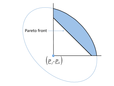
Figure 2 shows that the lower bound $\underline{v}_{1}$ (corresponding to an upper bound on $\ell$) does not affect the exactness of SOCP relaxation. The effect of upper bound $\overline{v}_{1}$ (corresponding to a lower bound on $\ell$) is illustrated in Figure 3. As explained in the caption of the figure SOCP relaxation is exact if the upper bound $\overline{v}_{1}$ does not exclude the high-voltage power flow solution $c$ and is not exact otherwise.

(a) Voltage constraint not binding

(b) Voltage constraint binding

Figure 3: Impact of voltage upper bound $\overline{v}_{1}$ on exactness. (a) When $\overline{v}_{1}$ (corresponding to a lower bound on $\ell$) is not binding, the power flow solution $c$ is in the feasible set of SOCP and hence the relaxation is exact. (b) When $\overline{v}_{1}$ excludes $c$ from the feasible set of SOCP, the optimal solution is infeasible for OPF and the relaxation is not exact.

To state the sufficient condition for a general radial network, recall from [25, Section VI] the linear approximation of BFM for radial networks obtained by setting $\ell_{jk}=0$ in (17): for each $s$

$$S^{\text{lin}}_{jk}(s) = \sum_{i\in\mathbb{T}_{j}}s_{i}$$ (22a)

$$v^{\text{lin}}_{j}(s) = v_{0}+2\sum_{(i,k)\in\mathbb{P}_{j}}\text{Re}\left(z_{ik}^{H}S_{ik}^{\text{lin}}(s)\right)$$ (22b)

where $\mathbb{T}_{j}$ denotes the subtree at node $j$, including $j$, and $\mathbb{P}_{j}$ denotes the set of links on the unique path from $j$ to $0$. The key property we will use is, from [25, Lemma 13 and Remark 9]:

$$S_{jk}\ \leq\ S_{jk}^{\text{lin}}(s) v_{j}\ \leq\ v_{j}^{\text{lin}}(s)$$ and (23)

Define the $2\times 2$ matrix function

$$A_{jk}(S_{jk},v_{j}) := I-\frac{2}{v_{j}}\,z_{jk}\left(S_{jk}\right)^{T}$$ (24)

where $z_{jk}:=[r_{jk}\ \,x_{jk}]^{T}$ is the line impedance and $S_{jk}:=[P_{jk}\ \,Q_{jk}]^{T}$ is the branch power flows, both taken as 2-dimensional real vectors so that $z_{jk}\left(S_{jk}\right)^{T}$ is a $2\times 2$ matrix with rank less or equal to 1. The matrices $A_{jk}(S_{jk},v_{j})$ describe how changes in the real and reactive power flows propagate towards the root node 0; see comments below. Evaluate the Jacobian matrix $A_{jk}(S_{jk},v_{j})$ at the boundary values:

$$\underline{A}_{jk} := A_{jk}\left(\left[S_{jk}^{\text{lin}}(\overline{s})\right]^{+}\!\!,\ \underline{v}_{j}\right)\ \,=\ \,I-\frac{2}{\underline{v}_{j}}\,z_{jk}\left(\left[S^{\text{lin}}_{jk}(\overline{s})\right]^{+}\right)^{T}$$ (25)

Here $\left(\left[a\right]^{+}\right)^{T}$ is the row vector $\left[[a_{1}]^{+}\ [a_{2}]^{+}\right]$ with $[a_{j}]^{+}:=\max\{0,a_{j}\}$.

For a radial network, for $j\neq 0$, every link $j\rightarrow k$ identifies a unique node $k$ and therefore, to simplify notation, we refer to a link interchangeably by $(j,k)$ or $j$ and use $A_{j}$, $\underline{A}_{j}$, $z_{j}$ etc. in place of $A_{jk}$, $\underline{A}_{jk}$, $z_{jk}$ etc. respectively.

Assume

1. The cost function is $C(x):=\sum_{j=0}^{n}C_{j}\left(\text{Re}\,s_{j}\right)$ with $C_{0}$ strictly increasing. There is no constraint on $s_{0}$.

2. The set $\mathbb{S}_{j}$ of injections satisfies $v_{j}^{\text{lin}}(s)\leq\overline{v}_{j}$, $j\in N$, where $v_{j}^{\text{lin}}(s)$ is given by (22).

3. For each leaf node $j\in N$ let the unique path from $j$ to 0 have $k$ links and be denoted by $\mathbb{P}_{j}:=((i_{k},i_{k-1}),\dots,(i_{1},i_{0}))$ with $i_{k}=j$ and $i_{0}=0$. Then $\underline{A}_{i_{t}}\cdots\underline{A}_{i_{t^{\prime}}}\,z_{i_{t^{\prime}+1}}>0$ for all $1\leq t\leq t^{\prime}<k$.

The following result is proved in [35].

Theorem 5

Suppose $\tilde{G}$ is a tree and B1–B3 hold. Then OPF-socp (19) is exact.

We now comment on the conditions B1–B3. B1 requires that the cost functions $C_{j}$ depend only on the injections $s_{j}$. For instance, if $C_{j}\left(\text{Re}\,s_{j}\right)=p_{j}$, then the cost is total active power loss over the network. It also requires that $C_{0}$ be strictly increasing but makes no assumption on $C_{j},j>0$. Common cost functions such as line loss or generation cost usually satisfy B1. If $C_{0}$ is only nondecreasing, rather than strictly increasing, in $p_{0}$ then B1–B3 still guarantee that all optimal solutions of OPF (10) are (effectively) optimal for OPF-socp (19), but OPF-socp may not be exact, i.e., it may have an optimal solution that maintains strict inequalities in (17c). In this case the proof of Theorem 5 can be used to recursively construct from it another optimal solution that attains equalities in (17c).

B2 is affine in the injections $s:=(p,q)$. It enforces the upper bounds on voltage magnitudes because of (23).

B3 is a technical assumption and has a simple interpretation: the branch power flow $S_{jk}$ on all branches should move in the same direction. Specifically, given a marginal change in the complex power on line $j\rightarrow k$, the $2\times 2$ matrix $\underline{A}_{jk}$ is (a lower bound on) the Jacobian and describes the effect of this marginal change on the complex power on the line immediately upstream from line $j\rightarrow k$. The product of $\underline{A}_{i}$ in B3 propagates this effect upstream towards the root. B3 requires that a small change, positive or negative, in the power flow on a line affects all upstream branch powers in the same direction. This seems to hold with a significant margin in practice; see [35] for examples from real systems.

Theorem 5 unifies and generalizes some earlier results in [32, 33, 34]. The sufficient conditions in these papers have the following simple and practical interpretation: OPF-socp is exact provided either

• there are no reverse power flows in the network, or

• if the $r/x$ ratios on all lines are equal, or

• if the $r/x$ ratios increase in the downstream direction from the substation (node 0) to the leaves then there are no reverse real power flows, or

• if the $r/x$ ratios decrease in the downstream direction then there are no reverse reactive power flows.

The exactness of SOCP relaxation does not require convexity, i.e., the cost $C(x)=\sum_{j=0}^{n}C_{j}(\text{Re}s_{j})$ need not be a convex function and the injection regions $\mathbb{S}_{j}$ need not be convex sets. Convexity allows polynomial-time computation. Moreover when it is convex the exactness of SOCP relaxation also implies the uniqueness of the optimal solution, as the following result from [35] shows.

Theorem 6

Suppose $\tilde{G}$ is a tree. Suppose the costs $C_{j}$, $j=0,\dots,n$, are convex functions and the injection regions $\mathbb{S}_{j}$, $j=1,\dots,n$, are convex sets. If the relaxation OPF-socp (19) is exact then its optimal solution is unique.

Consider the model of [18] for radial networks, which is (17) with the inequalities in (17c) replaced by equalities. Let $\mathbb{X}$ denote an equivalent feasible set of OPF, i.e., those $x\in\mathbb{R}^{3(m+n+1)}$ that satisfy (17), (18) and attain equalities in (17c). The proof of Theorem 6 reveals that, for radial networks, the feasible set $\mathbb{X}$ has a “hollow” interior.

Corollary 7

If $\hat{x}$ and $\tilde{x}$ are distinct solutions in $\mathbb{X}$ then no convex combination of $\hat{x}$ and $\tilde{x}$ can be in $\mathbb{X}$. In particular $\mathbb{X}$ is nonconvex.

This property is illustrated vividly in several numerical examples for mesh networks in [47, 48, 49, 50].

III-C Angle differences

The sufficient conditions in [29, 36, 37] require that the voltage angle difference across each line be small. We explain the intuition using a result in [36] for an OPF problem where $|V_{j}|$ are fixed for all $j\in N^{+}$ and reactive powers are ignored. Under these assumptions, as long as the voltage angle difference is small, the power flow solutions form a locally convex surface that is the Pareto front of its relaxation. This implies that the relaxation is exact. This geometric picture is apparent in earlier work on the geometry of power flow solutions, see e.g. [47], and underlies the intuition that the dynamics of a power system is usually benign until it is pushed towards the boundary of its stability region. The geometric insight in Figures 2 and 3 for BFM and later in this subsection for BIM says that, when it is far away from the boundary, the local convexity structure also facilitates exact relaxation. Reactive power is considered in [37, Theorem 1] with fixed $|V_{j}|$ where, with an additional constraint on the lower bounds of reactive power injections that ensure these lower bounds are not tight, it is proved that if the original OPF problem is feasible then its SDP relaxation is exact. The case of variable $|V_{j}|$ without reactive power is considered in [36, Theorem 7] but the simple geometric structure is lost.

Recall that $y_{jk}=g_{jk}-\textbf{i}b_{jk}$ with $g_{jk}>0,b_{jk}>0$. Let $V_{j}=|V_{j}|\,e^{\textbf{i}\theta_{j}}$ and suppose $|V_{j}|$ are given. Consider:

$$\min_{p,P,\theta} \!\!\!\!C(p)$$ (26a)

subject to $$\!\!\!\!\underline{p}_{j}\leq p_{j}\leq\overline{p}_{j},\qquad\quad\ \ j\in N^{+}$$ (26e)

$$\!\!\!\!\underline{\theta}_{jk}\leq\theta_{jk}\leq\overline{\theta}_{jk},\quad(j,k)\in E$$

$$\!\!\!\!p_{j}=\sum_{k:k\sim j}P_{jk},\qquad\quad\ \ j\in N^{+}$$

$$\!\!\!\!P_{jk}=|V_{j}|^{2}g_{jk}-|V_{j}||V_{k}|g_{jk}\cos\theta_{jk}+|V_{j}||V_{k}|b_{jk}\sin\theta_{jk},\quad(j,k)\in E$$

where $\theta_{jk}:=\theta_{j}-\theta_{k}$ are the voltage angle differences across lines $(j,k)$.

We comment on the constraints on angles $\theta_{jk}$ in (26). When the voltage magnitudes $|V_{i}|$ are fixed, constraints on real power flows, branch currents, line losses, as well as stability constraints can all be represented in terms of $\theta_{jk}$. Indeed a line flow constraint of the form $|P_{jk}|\leq\overline{P}_{jk}$ becomes a constraint on $\theta_{jk}$ using the expression for $P_{jk}$ in (26e). A current constraint of the form $|I_{jk}|\leq\overline{I}_{jk}$ is also a constraint on $\theta_{jk}$ since $|I_{jk}|^{2}=|y_{jk}|(|V_{j}|^{2}+|V_{k}|^{2}-2|V_{j}V_{k}|\cos\theta_{jk})$. The line loss over $(j,k)\in E$ is equal to $P_{jk}+P_{kj}$ which is again a function of $\theta_{jk}$. Stability typically requires $|\theta_{jk}|$ to stay within a small threshold. Therefore given constraints on branch power or current flows, losses, and stability, appropriate bounds $\underline{\theta}_{jk},\overline{\theta}_{jk}$ can be determined in terms of these constraints, assuming $|V_{j}|$ are fixed.

We can eliminate the branch flows $P_{jk}$ and angles $\theta_{jk}$ from (26). Since $|V_{j}|,j\in N^{+}$, are fixed we assume without loss of generality that $|V_{j}|=1$ pu. Define the injection region

$$\mathbb{P}_{\theta} \!\!\!\!\!:=\!\!\!\!\! \left\{p\in\mathbb{R}^{n}\left|p_{j}=\!\!\!\sum_{k:k\sim j}\!\!\left(g_{jk}-g_{jk}\cos\theta_{jk}+b_{jk}\sin\theta_{jk}\right),\,j\in N^{+},\ \underline{\theta}_{jk}\leq\theta_{jk}\leq\overline{\theta}_{jk},\,(j,k)\in E\right.\right\}$$ (27)

Let $\mathbb{P}_{p}:=\{p\in\mathbb{R}^{n}\,|\,\underline{p}_{j}\leq p_{j}\leq\overline{p}_{j},j\in N\}$. Then (26) is:
OPF:

$$\underset{p}{\min}\ C(p) p\in\mathbb{P}_{\theta}\cap\mathbb{P}_{p}$$ subject to (28)

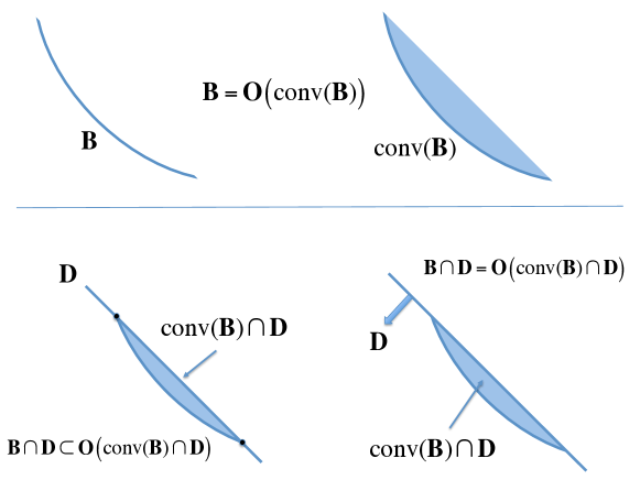
This problem is hard because the set $\mathbb{P}_{\theta}$ is nonconvex. To avoid triviality we assume OPF (28) is feasible. For a set $A$ let conv$\,A$ denote the convex hull of $A$. Consider the following problem that relaxes the nonconvex feasible set $\mathbb{P}_{\theta}\cap\mathbb{P}_{p}$ of (28) to a convex superset:
OPF-socp:

$$\underset{p}{\min}\ C(p) p\in\text{conv}(\mathbb{P}_{\theta})\,\cap\,\mathbb{P}_{p}$$ subject to (29)

We will show below that (29) is indeed an SOCP. It is said to be exact if every optimal solution of (29) lies in $\mathbb{P}_{\theta}\cap\mathbb{P}_{p}$ and is therefore also optimal for (28).

We say that a point $x\in A\subseteq\mathbb{R}^{n}$ is a Pareto optimal point in $A$ if there does not exist another $x^{\prime}\in A$ such that $x^{\prime}\leq x$ with at least one strictly smaller component $x_{j}^{\prime}<x_{j}$. The Pareto front of $A$, denoted by $\mathbb{O}(A)$, is the set of all Pareto optimal points in $A$. The significance of $\mathbb{O}(A)$ is that, for any increasing function, its minimizer, if exists, is necessarily in $\mathbb{O}(A)$ whether $A$ is convex or not. If $A$ is convex then $x^{\text{opt}}$ is a Pareto optimal point in $\mathbb{O}(A)$ if and only if there is a nonzero vector $c:=(c_{1},\dots,c_{n})\geq 0$ such that $x^{\text{opt}}$ is a minimizer of $c^{T}x$ over $A$ [51, pp.179–180].

Assume

1. $C(p)$ is strictly increasing in each $p_{j}$.

2. For all $(j,k)\in E$, $-\tan^{-1}\frac{b_{jk}}{g_{jk}}<\underline{\theta}_{jk}\leq\overline{\theta}_{jk}<\tan^{-1}\frac{b_{jk}}{g_{jk}}$.

The following result, proved in [36, 37], says that (29) is exact provided $\theta_{jk}$ are suitably bounded.

Theorem 8

Suppose $G$ is a tree and C1–C2 hold.

1. $\mathbb{P}_{\theta}\cap\mathbb{P}_{p}\ =\ \mathbb{O}(\text{conv}(\mathbb{P}_{\theta})\,\cap\,\mathbb{P}_{p})$.

2. The problem (29) is indeed an SOCP. Moreover it is exact.

C1 is needed to ensure every optimal solution of OPF-socp (29) is optimal for OPF (28). If $C(p)$ is nondecreasing but not strictly increasing in all $p_{j}$, then $\mathbb{P}_{\theta}\cap\mathbb{P}_{p}\subseteq\mathbb{O}(\text{conv}(\mathbb{P}_{\theta})\,\cap\,\mathbb{P}_{p})$ and OPF-socp may not be exact according to our definition. Even in that case it is possible to recover an optimal solution of OPF from any optimal solution of OPF-socp.

Theorem 8 is illustrated in Figures 4 and 5.

Figure 4: Feasible set of OPF (28) for a two-bus network without any constraint when $|V_{j}|$ are fixed and reactive powers are ignored. It is an ellipse without the interior, hence nonconvex. OPF-socp (29) includes the interior of the ellipse and is hence convex. If the cost function $C$ is strictly increasing in $(p_{j},p_{k})$ then the Pareto front of the SOCP feasible set will lie on the lower part of the ellipse, $\mathbb{O}(\mathbb{P}_{\theta})=\mathbb{P}_{\theta}$, and hence OPF-socp is exact.

(a) Exact relaxation with constraint

(b) Inexact relaxation with constraint

Figure 5: With lower bounds $\underline{p}$ on power injections, the feasible set of OPF-socp (29) is the shaded region. (a) When the feasible set of OPF (28) is restricted to the lower half of the ellipse (small $|\theta_{jk}|$), the Pareto front remains on the ellipse itself, $\mathbb{P}_{\theta}\cap\mathbb{P}_{p}=\mathbb{O}(\text{conv}(\mathbb{P}_{\theta})\,\cap\,\mathbb{P}_{p})$, and hence the relaxation is exact. (b) When the feasible set of OPF includes upper half of the ellipse (large $|\theta_{jk}|$), the Pareto front may not lie on the ellipse if $\underline{p}$ is large, making the relaxation not exact.

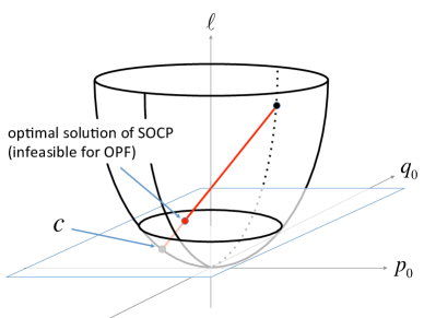
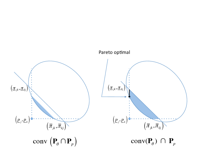
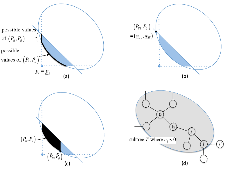
As explained in the caption of Figure 4, if there are no constraints then SOCP relaxation (29) is exact under condition C1. It is clear from the figure that upper bounds on power injections do not affect exactness whereas lower bounds do. The purpose of condition C2 is to restrict the angle $\theta_{jk}$ in order to eliminate the upper half of the ellipse from $\mathbb{P}_{\theta}$. As explained in the caption of Figure 5, under C2, $\mathbb{P}_{\theta}\cap\mathbb{P}_{p}=\mathbb{O}(\text{conv}(\mathbb{P}_{\theta})\,\cap\,\mathbb{P}_{p})$ and hence the relaxation is exact. Otherwise it may not.

When the network is not radial or $|V_{j}|$ are not constants, then the feasible set can be much more complicated than ellipsoids [48, 49, 50]. Even in such settings the Pareto fronts might still coincide, though the simple geometric picture is lost. See [47] for a numerical example on an Australian system or [24] on a three-bus mesh network.

III-D Equivalence

Since BIM and BFM are equivalent, the results on exact SOCP relaxation and uniqueness of optimal solution apply in both models. Recall the linear bijection $g$ from BIM to BFM defined in [25, end of Section V] by ${x}=g(W_{G})$ where

$$S_{jk} := y_{jk}^{H}\left([W_{G}]_{jj}-[W_{G}]_{jk}\right),\qquad\qquad\qquad\qquad\qquad\ \,\,j\rightarrow k\in\tilde{E}$$

$$\ell_{jk} \!\!\!:=\!\!\! |y_{jk}|^{2}\left([W_{G}]_{jj}+[W_{G}]_{kk}-[W_{G}]_{jk}-[W_{G}]_{kj}\right),\qquad\ j\rightarrow k\in\tilde{E}$$

$$v_{j} := [W_{G}]_{jj},\qquad\qquad\qquad\qquad\qquad\qquad\qquad\qquad\qquad\ \,j\in N^{+}$$

$$s_{j} := \sum_{k:j\sim k}y_{jk}^{H}\left([W_{G}]_{jj}-[W_{G}]_{jk}\right),\qquad\qquad\qquad\qquad\qquad\ \,\,j\in N^{+}$$

The mapping $g$ allows us to directly apply Theorem 6 to BIM. We summarize all the results for type A and type B conditions for radial networks.

Theorem 9

Suppose $G$ and $\tilde{G}$ are trees. Suppose conditions A1–A2’, or A3–A4, or B1–B3 hold. Then

1. BIM: SOCP relaxation (7) is exact. Moreover if $C(W_{G})$ is convex in $([W_{G}]_{jj},[W_{G}]_{jk})$ then the optimal solution is unique.

2. BFM: SOCP relaxation (13) is exact. Moreover if $C(x):=\sum_{j}C_{j}(p_{j})$ is convex in $p$ then the optimal solution is unique.

Since both the SDP and the chordal relaxations are equivalent to the SOCP relaxation for radial networks, these results apply to SDP and chordal relaxations as well.

IV Mesh networks

In this section we summarize a result of [17, Part II] on mesh networks with phase shifters and of [17, Part I], [39, 41] on dc networks when all voltages are nonnegative.

To be able to recover an optimal solution of OPF from an optimal solution $W_{G}^{\text{socp}}/x^{\text{socp}}$ of SOCP relaxation, $W_{G}^{\text{socp}}/x^{\text{socp}}$ must satisfy both a local condition and a global cycle condition ((4) for BIM and (12) for BFM); see the definition of exactness in Section II. The conditions of Section III guarantee that every SOCP optimal solution will satisfy the local condition (i.e., $W_{G}^{\text{socp}}$ is $2\times 2$ psd rank-1 and $x^{\text{socp}}$ attains equalities in (11c)), whether the network is radial or mesh, but do not guarantee that it satisfies the cycle condition. For radial networks, the cycle condition is vacuous and therefore the conditions of Section III are sufficient for SOCP relaxation to be exact. The result of [17, Part II] implies that these conditions are sufficient also for a mesh network that has tunable phase shifters at strategic locations.

Similar conditions also extend to dc networks where all variables are real and the voltages are assumed nonnegative.

IV-A AC networks with phase shifters

For BFM the conditions of Section III guarantee that every optimal solution of OPF-socp (13) attains equalities in (11c) but may or may not satisfy the cycle condition (12). If it does then it can be uniquely mapped to an optimal solution of OPF (10), according to [17, Theorem 2]. If it does not then the solution is not physically implementable because it does not satisfy the power flow equations (Kirchhoff’s laws). For a radial network the reduced incidence matrix $B$ in (12) is $n\times n$ and invertible and hence every optimal solution of the SOCP relaxation that attains equalities in (11c) always satisfies the cycle condition [17, Theorem 4]. This is not the case for a mesh network where $B$ is $m\times n$ with $m>n$.

It is proved in [17, Part II] however that if the network has tunable phase shifters then any SOCP solution that attains equalities in (11c) becomes implementable even if the solution does not satisfy the cycle condition. This extends the sufficient conditions A1–A2’, or A3–A4, or B1–B3, or C0–C1 from radial networks to this type of mesh networks.

For BIM the effect of phase shifter is equivalent to introducing a free variable $\phi_{c}$ in (4) for each basis cycle $c$ so that the cycle condition can always be satisfied for any $W_{G}$. The results presented here however start with a simple power flow model (30) for networks with phase shifters. This model makes transparent the effect of the spatial distribution of phase shifters and how they impact the exactness of SOCP relaxation and can be useful in other contexts, such as the design of a network of FACTS (Flexible AC Transmission Systems) devices.

BFM with phase shifters. We consider an idealized phase shifter that only shifts the phase angles of the sending-end voltage and current across a line, and has no impedance nor limits on the shifted angles. Specifically consider an idealized phase shifter parametrized by $\phi_{jk}$ across line $j\rightarrow k$ as shown in Figure 6.

Figure 6: Model of a phase shifter in line $j\rightarrow k$.

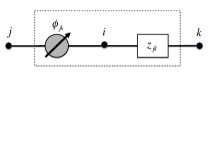
As before let $V_{j}$ denote the sending-end voltage at node $j$. Define $I_{jk}$ to be the sending-end current leaving node $j$ towards node $k$. Let $i$ be the point between the phase shifter $\phi_{jk}$ and line impedance $z_{jk}$. Let $V_{i}$ and $I_{i}$ be the voltage at $i$ and the current from $i$ to $k$ respectively. Then the effect of an idealized phase shifter, parametrized by $\phi_{jk}$, is summarized by the following modeling assumptions:

$$V_{i}\,=\,V_{j}\ e^{\textbf{i}\phi_{jk}} I_{i}\,=\,I_{jk}\ e^{\textbf{i}\phi_{jk}}$$ and

The power transferred from nodes $j$ to $k$ is still (defined to be) $S_{jk}:=V_{j}I_{jk}^{H}$, which is equal to the power $V_{i}I_{i}^{H}$ from nodes $i$ to $k$ since the phase shifter is assumed to be lossless. Applying Ohm’s law across $z_{jk}$, we define the branch flow model with phase shifters as the following set of equations:

$$\!\!\!\!\!\!\!\!\!\!\!\sum_{k:j\rightarrow k}\!\!S_{jk} \!\!\!=\!\!\! \!\!\sum_{i:i\rightarrow j}\!\!\left(S_{ij}-z_{ij}|I_{ij}|^{2}\right)+s_{j},\qquad j\in N^{+}$$ (30a)

$$\!\!\!\!\!\!\!\!\!\!\!I_{jk} \!\!\!=\!\!\! y_{jk}\left(V_{j}-V_{k}\ e^{-\textbf{i}\phi_{jk}}\right)\!,\quad\ j\rightarrow k\in\tilde{E}$$ (30b)

$$\!\!\!\!\!\!\!\!\!\!\!S_{jk} \!\!\!=\!\!\! V_{j}I_{jk}^{H},\qquad\qquad\qquad\quad\ j\rightarrow k\in\tilde{E}$$ (30c)

Without phase shifters ($\phi_{jk}=0$), (30) reduces to BFM (8). Let $\tilde{x}:=(S,I,V,s)\in\mathbb{C}^{2(m+n+1)}$ denote the variables in (30). Let $x:=(S,\ell,v,s)\in\mathbb{R}^{3(m+n+1)}$ denote the variables in SOCP relaxation (13). These variables are related through the mapping $x=h(\tilde{x})$ where $\ell_{jk}=|I_{jk}|^{2}$ and $v_{j}=|V_{j}|^{2}$. In particular, given any solution $\tilde{x}$ of (30), $x:=h(\tilde{x})$ satisfies (11) with equalities in (11c).

Cycle condition. If every line has a phase shifter then the cycle condition changes from (12) to: given any $x$ that satisfies (11) with equalities in (11c),

$$\!\!\!\!\!\!\exists(\theta,\phi)\in\mathbb{R}^{n+m} B\theta=\beta(x)-\phi\!\!\!\mod 2\pi$$ such that (31)

It is proved in [17, Part II] that, given any $x$ that attains equalities in (11c), there always exists a $\theta$ in $(-\pi,\pi]^{n}$ and a $\phi$ in $(-\pi,\pi]^{m}$ that solve (31). Moreover phase shifters are needed only on lines not in a spanning tree.

Exact SOCP relaxation. Recall the OPF problem (10) where the feasible set $\mathbb{\tilde{X}}$ without phase shifters is:

$$\mathbb{\tilde{X}} \!\!\!\!:=\!\!\!\! \{\tilde{x}\ |\ \tilde{x}\text{ satisfies }\eqref{eq:bfmps}\text{ with }\phi=0\text{ and }\eqref{eq:bfmopf}\}$$

Phase shifters on every line enlarge the feasible set to:

$$\overline{\mathbb{X}} \!:= \!\!\left\{\tilde{x}\ |\ \tilde{x}\text{ satisfies \eqref{eq:bfmps} for some $\phi$ and \eqref{eq:bfmopf}}\right\}$$

Given any spanning tree $T$ of $\tilde{G}$, let “$\phi\in T^{\perp}$” be the shorthand for “$\phi_{jk}=0$ for all $(j,k)\in T$”, i.e., $\phi$ involves only phase shifters in lines not in the spanning tree $T$. Fix any $T$. Define the feasible set when there are phase shifters only on lines outside $T$:

$$\overline{\mathbb{X}}_{T}\!\!\! \!\!\!:=\!\!\! \!\!\!\{\tilde{x}\ |\ \tilde{x}\text{ satisfies \eqref{eq:bfmps} for some $\phi\in T^{\perp}$ and \eqref{eq:bfmopf}}\}$$

Clearly $\tilde{\mathbb{X}}\subseteq\overline{\mathbb{X}}_{T}\subseteq\overline{\mathbb{X}}$. Define the (modified) OPF problem where there is a phase shifter on every line:
OPF-ps:

$$\min_{\tilde{x},\phi}\ C(x) \tilde{x}\in\overline{\mathbb{X}},\ \phi\in\mathbb{R}^{m}$$ subject to (32)

and that where there are phase shifters only outside $T$:
OPF-$T$:

$$\min_{\tilde{x},\phi}\ C(x) \tilde{x}\in\overline{\mathbb{X}}_{T},\ \phi\in T^{\perp}$$ subject to (33)

Let $C^{\text{opt}}$, $C^{\text{ps}}$, and $C^{T}$ denote respectively the optimal values of OPF (10), OPF-ps (32), and OPF-$T$ (33). Clearly $C^{\text{opt}}\geq C^{T}\geq C^{\text{ps}}$ since $\mathbb{\tilde{X}}\subseteq\overline{\mathbb{X}}_{T}\subseteq\overline{\mathbb{X}}$. Solving OPF (10), OPF-ps (32), or OPF-$T$ (33) is difficult because their feasible sets are nonconvex.

Recall the following sets defined in [25] for networks without phase shifters:

$$\mathbb{X}^{+} \!\!\!\!:=\!\!\!\! \{x\ |\ x\text{ satisfies \eqref{eq:bfmopf} and \eqref{eq:mdf}}\}$$

$$\mathbb{X}_{nc} \!\!\!\!:=\!\!\!\! \{x\ |\ x\text{ satisfies \eqref{eq:bfmopf} and \eqref{eq:mdf} with equalities in \eqref{eq:mdf.3}}\}$$

$$\mathbb{X} \!\!\!\!:=\!\!\!\! \{x\ |\ x\in\mathbb{X}_{nc}\text{ and satisfies the cycle condition \eqref{eq:cyclecond.1}}\}$$

Note that $\mathbb{X}$ is defined by the cycle condition without phase shifters $(\phi=0$ in (31)). As explained in [25, Theorem 9], $\mathbb{X}$ is equivalent to the feasible set $\mathbb{\tilde{X}}$ of OPF (10). Hence $\mathbb{\tilde{X}}\equiv\mathbb{X}\subseteq\mathbb{X}_{nc}\subseteq\mathbb{X}^{+}$. A key result of [17, Part II] is

Theorem 10

Fix any spanning tree $T$ of $\tilde{G}$. Then $\overline{\mathbb{X}}_{T}\ =\ \overline{\mathbb{X}}\ \equiv\ \mathbb{X}_{nc}$.

The implication of Theorem 10 is that, for a mesh network, when a solution of SOCP relaxation (13) attains equalities in (11c) (i.e., it is in $\mathbb{X}_{nc}$), then it can be implemented with an appropriate setting of phase shifters even when the solution does not satisfy the cycle condition (12). Define the problem:
OPF-nc:

$$\min_{x}\ C(x) x\in\mathbb{X}_{nc}$$ subject to (34)

Let $C^{\text{nc}}$ and $C^{\text{socp}}$ denote respectively the optimal values of OPF-nc (34) and OPF-socp (13). Theorem 10 then implies

Corollary 11

Fix any spanning tree $T$ of $\tilde{G}$. Then

1. $\mathbb{\tilde{X}}\subseteq\overline{\mathbb{X}}_{T}\ =\ \overline{\mathbb{X}}\ \equiv\ \mathbb{X}_{nc}\ \subseteq\ \mathbb{X}^{+}$.

2. $C^{\text{opt}}\geq C^{T}=C^{\text{ps}}=C^{\text{nc}}\geq C^{\text{socp}}$.

Hence if an optimal solution $x^{\text{socp}}$ of OPF-socp (13) attains equalities in (11c) then $x^{\text{socp}}$ solves the problem OPF-nc (34). If it also satisfies the cycle condition (12) then $x^{\text{socp}}\in\mathbb{X}$ and it can be mapped to a unique optimal of OPF (10). Otherwise, $x^{\text{socp}}$ can be implemented through an appropriate phase shifter setting $\phi$ and it attains a cost that lower bounds the optimal cost of the original OPF without tunable phase shifters. Moreover this benefit can be attained with phase shifters only outside an arbitrary spanning tree $T$ of $\tilde{G}$. The result can help determine if a network with a given set of phase shifters can be convexified and, if not, where additional phase shifters are needed for convexification [17, Part II].

Corollary 11 also implies that, if SOCP is exact, then phase shifters cannot further reduce the cost. This can help determine when phase shifters provide benefit to system operations.

Hence phase shifters in strategic locations make a mesh network behave like a radial network as far as convex relaxation is concerned. The results of Section III then imply

Corollary 12

Suppose conditions A1–A2’, or A3–A4, or B1–B3, or C1–C2 hold. Then any optimal solution of OPF-socp (13) solves OPF-ps (32) and OPF-$T$ (33).

IV-B DC networks

In this subsection we consider purely resistive dc networks, i.e., the impedance $z_{jk}=r_{jk}=y_{jk}^{-1}$, the power injections $s_{j}=p_{j}$, and the voltages $V_{j}$ are real. We assume all voltage magnitudes are strictly positive. Formally:

1. Replace (1b) and (11b) by $0<\underline{V}_{j}\leq V_{j}\leq\overline{V}_{j}$, $j\in N^{+}$, and replace (3b) by $0<\underline{V}_{j}^{2}\leq[W_{G}]_{jj}\leq\overline{V}_{j}^{2}$, $j\in N^{+}$.

Type A conditions. Condition D0 immediately implies that the cycle condition (12) in BFM is satisfied by every feasible $x$ of OPF-socp (13), for

$$\beta_{jk}(x) := \angle\left(v_{j}-z_{jk}^{H}S_{jk}\right)\ \ =\ \ \angle\left(v_{j}-r_{jk}\left(r_{jk}^{-1}V_{j}(V_{j}-V_{k})\right)\right)\ \ =\ \ 0$$

A3–A4 guarantee that any optimal solution of OPF-socp attains equality in (11c) for general mesh networks. Hence [25, Theorem 7] and Theorem 4 imply

Corollary 13

Suppose A3–A4 and D0 hold. Then OPF-socp (13) is exact.

For BIM, consider an OPF as a QCQP (16) where all the matrices are real and symmetric. Even though all the QCQP matrices in (16) satisfy condition A2’, Corollary 3 is not directly applicable as its proof constructs a complex (rather than real) $V$ from an optimal solution of OPF-socp. However if there are no lower bounds on the power injections, then only $\Phi_{j}$ are involved in the QCQP so all their off-diagonal entries are negative. It is then observed in [39] that [45, Theorem 3.1] directly implies (without needing D0)

Corollary 14

Suppose A1 and A4 hold. Then OPF-sdp (5) and OPF-socp (7) are exact.

Type B conditions. The following result is proved in [41]. Consider:

1. The cost function is $C(x):=\sum_{j=0}^{n}C_{j}\left(\text{Re}\,s_{j}\right)$ with $C_{j}$ strictly increasing for all $j\in N^{+}$. There is no constraint on $s_{0}$.

2. $\overline{V}_{1}=\overline{V}_{2}=\cdots=\overline{V}_{n}$; $\mathbb{S}_{j}=[\underline{p}_{j},\overline{p}_{j}]$ with $\underline{p}_{j}<0$, $j\in N$.

3. $\overline{V}_{j}=\infty$ for $j\in N$.

Theorem 15

Suppose at least one of the following holds:

• B1, B2” and D0; or

• B1’, B2’ and D0.

Then OPF-socp (7) with the additional constraints $W_{jk}\geq 0$, $(j,k)\in E$, is exact. If, in addition, the problem is convex then its optimal solution is unique.

It is possible to enforce B2” by an affine constraint on the power injections, similar to (but different from) condition B2 for radial networks; see [41] for details. See also [52] for a result on the uniqueness of SOCP relaxation.

IV-C General AC networks

Unfortunately no sufficient conditions for exact semidefinite relaxation for general mesh networks are yet known. There are type A conditions on power injections for exact relaxation only for special cases: a lossless cycle or lossless cycle with one chord [29], or a weakly cyclic network (where every line belongs to at most one cycle) of size 3 [53].

We close by mentioning three recent approaches for global optimization of OPF when the relaxations in this tutorial fail. First, higher-order semidefinite relaxations on the Lesserre hierarchy for polynomial optimization [54] have been applied to solving OPF when SDP relaxation fails [55, 56, 57, 58]. By going up the hierarchy, the relaxations become tighter and their solutions approach a global optimal of the original polynomial optimization [54, 59]. This however comes at the cost of significantly higher runtime. Techniques are proposed in [57, 58] to reduce the problem sizes, e.g., by exploiting sparsity or adding redundant constraints [60, 61, 58] or applying higher-order relaxations only on (typically small) subnetworks where constraints are violated [57].

Second, a branch-and bound algorithm is proposed in [62] where a lower bound is computed from the Lagrangian dual of OPF and the feasible set subdivision is based on rectangular or ellipsoidal bisection. The dual problem is solved using a subgradient algorithm. Each iteration of the subgradient algorithm requires minimizing the Lagrangian over the primal variables. This minimization is separable into two subproblems, one being a convex subproblem and the other having a nonconvex quadratic objective. The latter subproblem turns out to be a trust-region problem that has a closed-form solution. It is proved in [62] that the proposed algorithm converges to a global optimal. This method is extended in [63] to include more constraints and alternatively use SDP relaxation for lower bounding the cost.

Finally a new approach is proposed in [64] based on convex quadratic relaxation of OPF in polar coordinates.

V Conclusion

We have summarized the main sufficient conditions for exact semidefintie relaxations of OPF as listed in Tables II and II. For radial networks these conditions suggest that SOCP relaxation (and hence SDP and chordal relaxations) will likely be exact in practice. This is corroborated by significant numerical experience. For mesh networks they are applicable only for special cases: networks that have tunable phase shifters or dc networks where all variables are real and voltages are nonnegative. Even though counterexamples exist where SDP/chordal relaxation is not exact for AC mesh networks numerical experience seems to suggest that SDP/chordal relaxation tends to be exact in many cases. Sufficient conditions that guarantee exact relaxation for AC mesh networks however remain elusive. The main difficulty is in designing relaxations of the cycle condition (4) or (12).

VI Appendix: proofs

We prove all the main results here.

VI-A Proof of Theorem 1 and Corollary 2: linear separability

The proof is from an updated version of [27]. It is equivalent to the argument of [31] and simpler than the original duality proof in [27].

Proof:

Fix any partial matrix $W_{G}$ that is feasible for SOCP (15). We will construct an $x\in\mathbb{C}^{n+1}$ that satisfies

$$x^{H}C_{l}x \leq \text{tr }C_{l}W_{G},\ \ \ l=0,1,\dots,L$$

i.e., $x$ is feasible for QCQP (14) and has an equal or lower cost than $W_{G}$. Since the minimum cost of QCQP is lower bounded by that of its SOCP relaxation this means that an optimal solution $x\in\mathbb{C}^{n+1}$ of QCQP (14) can be obtained from every optimal solution $W_{G}$ of SOCP (15).

Now $W_{G}(j,k)\succeq 0$ for every $(j,k)\in E$ implies that $[W_{G}]_{jj}\geq 0$ for all $j\in N$ and

$$[W_{G}]_{jj}\,[W_{G}]_{kk} \geq \left|[W_{G}]_{jk}\right|^{2},\ \ (j,k)\in E$$

Suppose first that $[W_{G}]_{jj}[W_{G}]_{kk}=|[W_{G}]_{jk}|^{2}$ for all $(j,k)\in E$, i.e., $W_{G}$ is $2\times 2$ psd rank-1. We will construct an $x\in\mathbb{C}^{n+1}$ that is feasible for QCQP and has an equal cost. To construct such an $x$ let $|x_{j}|:=\sqrt{[W_{G}]_{jj}}$, $j\in N^{+}$. Recall that $G$ is a (connected) tree with node 0 as its root. Let $\angle x_{0}:=0$. Traversing the tree starting from the root the angles can be successively assigned: given $\angle x_{j}$ at one end of a link $(j,k)$, let $\angle x_{k}:=\angle x_{j}-\angle[W_{G}]_{jk}$ at the other end. Then for $l=0,1,\dots,L$ we have

$$x^{H}C_{l}x = \sum_{j,k}[C_{l}]_{jk}\,x_{j}x_{k}^{H}\ =\ \text{tr }C_{l}W_{G}$$

Hence $x$ is feasible for QCQP (14) and has the same cost as $W_{G}$.

Next suppose $[W_{G}]_{jj}[W_{G}]_{kk}>|[W_{G}]_{jk}|^{2}$ for some $(j,k)$, i.e., $W_{G}$ is $2\times 2$ psd but not $2\times 2$ rank-1. We will

1. Construct an $\hat{W}_{G}$ that is $2\times 2$ psd rank-1.

2. Show that A2 implies

   $$\text{tr }C_{l}\hat{W}_{G} \leq \text{tr }C_{l}W_{G},\ \ l=0,1,\dots,L$$ (35)

Then an $x\in\mathbb{C}^{n+1}$ can be constructed from $\hat{W}_{G}$ as in the case above and step 2 ensures that for $l=0,1,\dots,L$

$$x^{H}C_{l}x\ =\ \text{tr }C_{l}\hat{W}_{G}\ \leq\ \text{tr }C_{l}W_{G}$$

i.e., $x$ is feasible for QCQP (14) and has an equal or lower cost than $W_{G}$.

To construct such an $\hat{W}_{G}$ let $[\hat{W}_{G}]_{jj}=[W_{G}]_{jj}$, $j\in N^{+}$. For $(j,k)\in E$ let

$$[\hat{W}_{G}]_{jk}-[W_{G}]_{jk} =: r_{jk}e^{-\textbf{i}\left(\frac{\pi}{2}-\alpha_{jk}\right)}$$

for some $r_{jk}>0$ to be determined and $\alpha_{jk}$ in assumption A2. For $\hat{W}_{G}$ to be $2\times 2$ psd rank-1 we need to choose $r_{jk}>0$ such that $[\hat{W}_{G}]_{jj}[\hat{W}_{G}]_{kk}=\left|[\hat{W}_{G}]_{jk}\right|^{2}$ for all $(j,k)\in E$, i.e.,

$$[W_{G}]_{jj}\,[W_{G}]_{kk} = \left|[W_{G}]_{jk}+r_{jk}e^{-\textbf{i}\left(\frac{\pi}{2}-\alpha_{jk}\right)}\right|^{2}$$

or

$$r_{jk}^{2}+2b\,r_{jk}-c = 0$$

where

$$b := \text{Re}\left([W_{G}]_{jk}\,e^{\textbf{i}\left(\frac{\pi}{2}-\alpha_{jk}\right)}\right)$$

$$c := [W_{G}]_{jj}\,[W_{G}]_{kk}-\left|[W_{G}]_{jk}\right|^{2}\ >\ 0$$

Therefore setting $r_{jk}:=\sqrt{b^{2}+c}-b>0$ yields an $\hat{W}_{G}$ that is $2\times 2$ psd rank-1.

To show that $\hat{W}_{G}$ is feasible for SOCP (15) and has an equal or lower cost than $W_{G}$, we have for $l=0,1,\dots,L$,

$$\text{tr }C_{l}\hat{W}_{G}-\text{tr }C_{l}W_{G} = \text{tr }C_{l}\,\left(\hat{W}_{G}-W_{G}\right)$$

$$= \sum_{(j,k)\in E}[C_{l}]_{jk}\left([\hat{W}_{G}]_{jk}-[W_{G}]_{jk}\right)^{H}$$

$$= 2\,\sum_{j<k}\text{Re}\left([C_{l}]_{jk}\cdot r_{jk}\,e^{\textbf{i}\left(\frac{\pi}{2}-\alpha_{jk}\right)}\right)$$

$$= 2\,\sum_{j<k}\left|[C_{l}]_{jk}\right|\,r_{jk}\ \cos\left(\angle[C_{l}]_{jk}+\frac{\pi}{2}-\alpha_{jk}\right)$$

$$\leq 0$$

where the last inequality follows because assumption A2 implies

$$\frac{\pi}{2} \leq\ \,\angle[C_{l}]_{jk}+\frac{\pi}{2}-\alpha_{jk}\ \,\leq \frac{3\pi}{2}$$

and therefore $\cos\left(\angle[C_{l}]_{jk}+\frac{\pi}{2}-\alpha_{jk}\right)\leq 0$. This completes the proof. ∎

Proof:

A1 implies that the objective function of SOCP (15) is strictly convex and hence has a unique optimal solution. Suppose $W_{G}$ is an optimal solution of SOCP (15) but $[W_{G}]_{jj}[W_{G}]_{kk}>|[W_{G}]_{jk}|^{2}$ for some $(j,k)$, i.e., $W_{G}$ is $2\times 2$ psd but not $2\times 2$ psd rank-1. Then the above constructs another feasible solution $\hat{W}_{G}$ with equal cost. This contradicts the uniqueness of the optimal solution of SOCP (15), and hence $W_{G}$ must be $2\times 2$ psd rank-1. ∎

VI-B Proof of Theorem 4: no injection lower bounds (BFM)

The proof is from [17, Part I].

Proof:

Fix any optimal solution $x:=(S,\ell,v,s)\in\mathbb{R}^{3(m+n+1)}$ of OPF-socp in the branch flow model. Since the network is radial, the cycle condition is vacuous and we only need to show that $x$ attains equality in (11c) on all lines $j\rightarrow k\in\tilde{E}$. For the sake of contradiction assume this is violated on $j\rightarrow$k, i.e.,

$$v_{j}\ell_{jk} > |S_{jk}|^{2}$$ (36)

We will construct an $\hat{x}$ that is feasible for OPF-socp and attains a strictly lower cost, contradicting that $x$ is optimal.

For an $\epsilon>0$ to be determined below, consider the following $\hat{x}$ obtained by modifying only the current $\ell_{jk}$ and power flows $S_{jk}$ on line $j\rightarrow k$ and the injections $s_{j},s_{k}$ at two ends of the line:

$$\hat{\ell}_{jk} := \ell_{jk}-\epsilon$$

$$\hat{S}_{jk} := S_{jk}-z_{jk}\epsilon/2$$

$$\hat{s}_{j} := s_{j}-z_{jk}\epsilon/2$$

$$\hat{s}_{k} := s_{k}-z_{jk}\epsilon/2$$

and $\hat{v}\ :=\ v$, $\hat{\ell}_{il}\ :=\ \ell_{il}$ and $\hat{S}_{il}\ :=\ S_{il}$ for $(i,l)\neq(j,k)$, $\hat{s}_{i}:=s_{i}$ for $i\neq j,k$. By assumption A3 the objective function $C(x)$ is strictly increasing in $\ell$ and hence $\hat{x}$ has a strictly lower cost than $x$. It suffices to show that there exists an $\epsilon>0$ such that $\hat{x}$ is feasible for OPF-socp, i.e., $\hat{x}$ satisfies (11) and (9).

Assumption A4 ensures that $\hat{x}$ satisfies (9). Further $\hat{x}$ satisfies (11a) at buses $i\neq j,k$, and satisfies (11b) and (11c) over lines $(i,l)\neq(j,k)$. We now show that $\hat{x}$ also satisfies (11a) at buses $j$ and $k$ and satisfies (11b) and (11c) over line $(j,k)$.

For (11a) at bus $j$, we have (adopting the graph orientation where every link points away from node 0):

$$\sum_{l:j\rightarrow l}\hat{S}_{jl} = \sum_{l\neq k:j\rightarrow l}S_{jl}+\left(S_{jk}-z_{jk}\epsilon/2\right)\ \ =\ \ S_{ij}-z_{ij}\ell_{ij}+s_{j}-z_{jk}\epsilon/2\ \,=\,\ \hat{S}_{ij}-z_{ij}\hat{\ell}_{ij}+\hat{s}_{j}$$

as desired. For (11a) at $k$, we have

$$\sum_{l:k\rightarrow l}\hat{S}_{kl} = \sum_{l:k\rightarrow l}S_{kl}\ =\ S_{jk}-z_{jk}\ell_{jk}+s_{k}\ \ =\ \ \hat{S}_{jk}-z_{jk}\hat{\ell}_{jk}+\hat{s}_{k}$$

as desired. For (11b) over line $(j,k)$, we have

$$\hat{v}_{j}-\hat{v}_{k} = v_{j}-v_{k}\ \ =\ \ 2\,\text{Re}\left(z_{jk}^{H}S_{jk}\right)-|z_{jk}|^{2}\ell_{jk}\ \ =\ \ 2\,\text{Re}\left(z_{jk}^{H}\hat{S}_{jk}\right)-|z_{jk}|^{2}\hat{\ell}_{jk}$$

as desired. For (11c) over line $(j,k)$, we have

$$\hat{v}_{j}\hat{\ell}_{jk}-\left|\hat{S}_{jk}\right|^{2} = -\frac{\left|z_{jk}\right|^{2}}{4}\epsilon^{2}\ -\,\left(\!v_{j}-\text{Re}\left(z_{jk}^{H}S_{jk}\right)\right)\epsilon\ +\ \left(\ell_{jk}v_{j}-\left|S_{jk}\right|^{2}\right)$$

Hence (36) implies that we can always choose an $\epsilon>0$ such that $\hat{v}_{j}\hat{\ell}_{jk}=\left|\hat{S}_{jk}\right|^{2}$. This completes the proof. ∎

If the cost function $C(x)$ in A3 is only nondecreasing, rather than strictly increasing, in $\ell$, then A3–A4 still guarantee that all optimal solutions of OPF (10) are optimal for OPF-socp (13), but OPF-socp (13) may have optimal solutions $x$ that maintain strict inequalities in (11c). Even in this case, however, the above proof constructs from $x$ an optimal solution $\hat{x}$ of OPF-socp that attains equalities in (11c) from which an optimal solution $\tilde{x}$ of OPF (10) can be recovered.

VI-C Proof of Theorem 5: voltage upper bounds

The proof here is from [35] with a slightly different presentation. Given an optimal solution $x$ that maintains a strict inequality in (11c), the proof in Section VI-B of Theorem 4 by contradiction constructs another feasible solution $\hat{x}$ that incurs a strictly smaller cost, contradicting the optimality of $x$. The modification is over a single line over which $x$ maintains a strict inequality in (11c). The proof of Theorem 5 is also by contradiction but, unlike that of Theorem 4, the construction of $\hat{x}$ from $x$ involves modifications on multiple lines, propagating from the line that is closest to bus 0 where (11c) holds with strict inequality all the way to bus 0. The proof relies crucially on the recursive structure of the branch flow model (17).

Proof:

To simplify notation we only prove the theorem for the case of a linear network representing a primary feeder without laterals. The proof for a general tree network follows the same idea but with more cumbersome notations; see [35] for details. We adopt the graph orientation where every link points towards the root node 0. The notation for the linear network is explained in Figure 7 (recall that we refer to a link $j\rightarrow k$ by $j$ and index the associated variables $z_{jk},S_{jk},\ell_{jk}$ with $j$).

Figure 7: Linear network and notations. Line $m$ in the proof is the line closest to bus 0 where the inequality in (38) is strict, i.e., (38) holds with equality at lines $j=1,\dots,m-1$, strict inequality at line $m$, and inequality at lines $j=m+1,\dots,n$.

With this notation the branch flow model (17) is the following recursion:

$${S}_{j-1} = {S}_{j}-z_{j}\ell_{j}+s_{j-1},\qquad\qquad\quad\!j=1,\dots,n$$ (37a)

$$v_{j-1} = v_{j}-2\,\text{Re}\left(z_{j}^{H}S_{j}\right)+|z_{j}|^{2}\ell_{j},\quad j=1,\dots,n$$ (37b)

$$v_{j}\ell_{j} = |S_{j}|^{2},\qquad\qquad\qquad\qquad\quad\ j=1,\dots,n$$ (37c)

$$S_{n} = s_{n},\qquad S_{0}:=0$$ (37d)

where $v_{0}$ is given. The SOCP relaxation of (37c) is:

$$v_{j}\ell_{j} \geq |S_{j}|^{2},\qquad j=1,\dots,n$$ (38)

OPF on the linear network then becomes ($s_{0}$ is unconstrained by assumption B1):
OPF:

$$\underset{x}{\text{min}} C(x):=\sum_{j=0}^{n}C_{j}\left(\text{Re }s_{j}\right)$$ (39a)

subject to $$x\text{ satisfies \eqref{eq:cnstrs} and \eqref{eq:lndf} }$$ (39b)

and its SOCP relaxation becomes:
OPF-socp:

$$\underset{x}{\text{min}} C(x):=\sum_{j=0}^{n}C_{j}\left(\text{Re }s_{j}\right)$$

subject to $$x\text{ satisfies \eqref{eq:cnstrs} and }\text{\eqref{eq:lndf} with \eqref{eq:lndf.3} replaced by \eqref{eq:lndf.socp}}$$ (40a)

For the linear network assumption B3 reduces:

1. $\underline{A}_{j}\cdots\underline{A}_{k}\ z_{k+1}>0$ for $1\leq j\leq k<n$.

Our goal is to prove OPF-socp (40) is exact, i.e., every optimal solution of (40) attains equality in (38) and hence is also optimal for OPF (39). Suppose on the contrary that there is an optimal solution $x:=(S,\ell,v,s)$ of OPF-socp (40) that violates (37c). We will construct another feasible point $\hat{x}:=(\hat{S},\hat{\ell},\hat{v},\hat{s})$ of OPF-socp (40) that has a strictly lower cost than $x$, contradicting the optimality of $x$.

Let $m:=\min\,\{j\in N\ |\ v_{j}\ell_{j}>|S_{j}|^{2}\}$ be the closest link from bus 0 where (37c) is violated; see Figure 7. Pick any $\epsilon_{m}\in(0,\ell_{m}-|S_{m}|^{2}/v_{m}]$ and construct $\hat{x}$ as follows:

1. $\hat{s}_{j}:=s_{j}$ for $j\neq 0$.

2. For $\hat{S},\hat{\ell},\hat{s}_{0}$:

   • For $j=n,\dots,m+1$: $\hat{S}_{j}:=S_{j}$ and $\hat{\ell}_{j}:=\ell_{j}$.

   • For $j=m$: $\hat{S}_{m}:=S_{m}$ and $\hat{\ell}_{m}:=\ell_{m}-\epsilon_{m}$.

   • For $j=m-1,\dots,1$:

     $$\hat{S}_{j} := \hat{S}_{j+1}-z_{j+1}\hat{\ell}_{j+1}+\hat{s}_{j}$$

     $$\hat{\ell}_{j} := \frac{|\hat{S}_{j}|^{2}}{v_{j}}$$

   • $\hat{s}_{0}:=-\hat{S}_{1}+z_{1}\hat{\ell}_{1}$.

3. $\hat{v}_{0}:=v_{0}$. For $j=1,\dots,n$,

   $$\hat{v}_{j} := \hat{v}_{j-1}+2\,\text{Re}\left(z_{j}^{H}\hat{S}_{j}\right)-|z_{j}|^{2}\hat{\ell}_{j}$$

Notice that the denomintor in $\hat{\ell}_{j}$ is defined to be $v_{j}$, not $\hat{v}_{j}$. This decouples the recursive construction of $(\hat{S}_{j},\hat{\ell}_{j})$ and $\hat{v}_{j}$ so that the former propagates from bus $n$ towards bus 1 while the latter propagates in the opposite direction.

By construction $\hat{x}$ satisfies (37a), (37b), (37d), and (18b). We only have to prove that $\hat{x}$ satisfies (18a) and (38). Hence the proof of Theorem 5 is complete after Lemma 16 is established, which asserts that $\hat{x}$ is feasible and has a strictly lower cost under assumptions B1, B2, B3’.

Lemma 16

Under the conditions of Theorem 5 $\hat{x}$ satisfies

1. $C(\hat{x})\ <\ C(x)$.

2. $\hat{v}_{j}\hat{\ell}_{j}\ \geq\ \left|\hat{S}_{j}\right|^{2}$, $j\in N$.

3. $\underline{v_{j}}\ \leq\ \hat{v}_{j}\ \leq\ \overline{v}_{j}$, $j\in N$.

To simplify the notation redefine $S_{0}:=-s_{0}$ and $\hat{S}_{0}:=-\hat{s}_{0}$. Then for $j\in N^{+}$ define $\Delta S_{j}:=\hat{S}_{j}-S_{j}$ and $\Delta v_{j}:=\hat{v}_{j}-v_{j}$. The key result that leads to Lemma 16 is:

$$\Delta S_{j}\ \geq\ 0 \Delta v_{j}\ \geq\ 0$$ and

The first inequality is stated more precisely in Lemma 17 and proved after the proof of Lemma 16.

Lemma 17

Suppose $m>1$ and B3’ holds. Then $\Delta S_{j}\geq 0$ for $j\in N^{+}$ with $\hat{S}_{j}>S_{j}$ for $j=0,\dots,m-1$. In particular $\hat{s}_{0}<s_{0}$.

We now prove the second inequality together with Lemma 16 assuming Lemma 17 holds.

Proof:

1) If $m=1$ then, by construction, $\hat{s}_{0}=s_{0}-z_{1}\epsilon_{1}<s_{0}$ since $z_{1}>0$. If $m>1$ then $\hat{s}_{0}<s_{0}$ by Lemma 17. Since $\hat{s}=s$ and $\hat{s}_{0}<s_{0}$ we have

$$C(\hat{x})-C(x) = \sum_{j=0}^{n}\left(C_{j}\left(\text{Re }\hat{s}_{j}\right)-C_{j}\left(\text{Re }s_{j}\right)\right)\ \,=\ \,C_{0}\left(\text{Re }\hat{s}_{0}\right)-C_{0}\left(\text{Re }s_{0}\right)\ \ <\ \ 0$$

as desired, since $C_{0}$ is strictly increasing.

2) To avoid circular argument we will first prove using Lemma 17

$$\hat{v}_{j} \geq v_{j},\qquad\quad j\in N$$ (41)

We will then use this and Lemma 17 to prove $\hat{v}_{j}\hat{\ell}_{j}\geq|\hat{S}_{j}|^{2}$ for all $j\in N$. This means that $\hat{x}$ satisfies (37a), (37b), and (38). We can then use [25, Lemma 13] and assumption B2 to prove $\underline{v_{j}}\ \leq\ \hat{v}_{j}\ \leq\ \overline{v}_{j}$, $j\in N$.

To prove (41), note that both $\hat{v}$ and $v$ satisfy (37b) and hence we have, for $j=1,\dots,n$,

$$\Delta v_{j-1} = \Delta v_{j}-2\,\text{Re}\left(z_{j}^{H}\Delta S_{j}\right)+|z_{j}|^{2}\Delta\ell_{j}\qquad$$ (42)

where $\Delta\ell_{j}:=\hat{\ell}_{j}-\ell_{j}$. From (37a) we have

$$z_{j}\Delta\ell_{j} = \Delta S_{j}-\Delta S_{j-1}+\Delta s_{j-1}$$

where $\Delta s_{0}:=\hat{s}_{0}-s_{0}<0$ and $s_{j-1}=0$ for $j>1$. Multiplying both sides by $z_{j}^{H}$ and noticing that both sides must be real, we conclude

$$|z_{j}|^{2}\Delta\ell_{j} = \text{Re }\left(z_{j}^{H}\Delta S_{j}-z_{j}^{H}\Delta S_{j-1}+z_{j}^{H}\Delta s_{j-1}\right)$$

Substituting into (42) we have for $j=1,\dots,n$

$$\Delta v_{j}-\Delta v_{j-1} \!\!\!=\!\!\! \text{Re }z_{j}^{H}\Delta S_{j}\ +\ \text{Re }z_{j}^{H}\Delta S_{j-1}\ -\ \text{Re }z_{j}^{H}\Delta s_{j-1}$$

But Lemma 17 implies that $\text{Re }z_{j}^{H}\Delta S_{j}=r_{j}\,\Delta P_{j}+x_{j}\,\Delta Q_{j}\geq 0$. Similarly every term on the right-hand side is nonnegative and hence

$$\Delta v_{j} \geq \Delta v_{j-1}\qquad\text{ for }j=1,\dots,n$$

implying that $\Delta v_{j}\geq\Delta v_{0}=0$, proving (41).

We now use (41) to prove the second assertion of the lemma. By construction, for $j=m+1,\dots,n$,

$$\hat{\ell}_{j} = \ell_{j}\ \geq\ \frac{|S_{j}|^{2}}{v_{j}}\ \geq\ \frac{|\hat{S}_{j}|^{2}}{\hat{v}_{j}}$$

as desired, since $\hat{S}_{j}=S_{j}$ and $\hat{v}_{j}\geq v_{j}$. Similarly (38) holds for $\hat{x}$ for $j=m$ because of the choice of $\epsilon_{m}$. For $j=1,\dots,m-1$, $\hat{v}_{j}\geq v_{j}$ again implies

$$\hat{\ell}_{j} = \frac{|\hat{S}_{j}|^{2}}{v_{j}}\ \geq\ \frac{|\hat{S}_{j}|^{2}}{\hat{v}_{j}}$$

3) The relation (41) means

$$\hat{v}_{j} \geq v_{j}\ \geq\ \underline{v}_{j},\qquad j\in N$$

Assumption B2 and [25, Lemma 13] (see also Remark 6 of [25]) imply that

$$\hat{v}_{j} \leq v_{j}^{\text{lin}}(s)\ \leq\ \overline{v}_{j},\qquad j\in N$$

This proves $\hat{x}$ satisfies (18a) and completes the proof of Lemma 16. ∎

The remainder of this subsection is devoted to proving the key result Lemma 17.

Proof:

By construction $\Delta S_{j}=0$ for $j=m,\dots,n$. To prove $\Delta S_{j}>0$ for $j=0,\dots,m-1$, the key idea is to derive a recursion on $\Delta S_{j}$ in terms of the Jacobian matrix $A_{j}(S_{j},v_{j})$. The intuition is that, when the branch current $\ell_{m}$ is reduced by $\epsilon_{m}$ to $\hat{\ell}_{m}$, loss on line $m$ is reduced and all upstream branch powers $S_{j}$ will be increased to $\hat{S}_{j}$ as a consequence.

This is proved in three steps, of which we now give an informal overview. First we derive a recursion (44) on $\Delta S_{j}$. This motivates a collection of linear dynamical systems $w$ in (46) that contains the process $(\Delta S_{j}$, $j=0,\dots,m-1)$ as a specific trajectory. Second we construct another collection of linear dynamical systems $\underline{w}$ in (47) such that assumption B3’ implies $\underline{w}>0$. Finally we prove an expression for the process $w-\underline{w}$ that shows $w\geq\underline{w}$ (in Lemmas 18, 19, 20). This then implies $\Delta S=w\geq\underline{w}>0$. We now make these steps precise.

Since both $x$ and $\hat{x}$ satisfy (37a) and $\hat{s}_{j}=s_{j}$ for all $j\in N$ we have (with the redefined $\Delta S_{0}:=-(\hat{s}_{0}-s_{0})$)

$$\Delta{S}_{j-1} = \Delta{S}_{j}-z_{j}\Delta\ell_{j},\quad j=1,2,\dots,n\qquad$$ (43)

where $\Delta\ell_{j}:=\hat{\ell}_{j}-\ell_{j}$. For $j=1,\dots,m-1$ both $x$ and $\hat{x}$ satisfy (37c). For these $j$, fix any $v_{j}\geq\underline{v}_{j}$ and consider $\ell_{j}:=\ell_{j}(S_{j})$ as functions of the real pair $S_{j}:=(P_{j},Q_{j})$:

$$\ell_{j}(S_{j}) := \frac{P_{j}^{2}+Q_{j}^{2}}{v_{j}},\quad j=1,\dots,m-1$$

whose Jacobian are the row vectors:

$$\frac{\partial\ell_{j}}{\partial S_{j}}(S_{j}) = \frac{2}{v_{j}}[P_{j}\ \ Q_{j}]\ =\ \frac{2}{v_{j}}S_{j}^{T}$$

The mean value theorem implies for $j=1,\dots,m-1$

$$\Delta\ell_{j} = \ell_{j}(\hat{S}_{j})-\ell_{j}(S_{j})\ =\ \frac{\partial\ell_{j}}{\partial S_{j}}(\tilde{S}_{j})\,\Delta S_{j}$$

where $\tilde{S}_{j}:=\alpha_{j}S_{j}+(1-\alpha_{j})\hat{S}_{j}$ for some $\alpha_{j}\in[0,1]$. Substituting it into (43) we obtain the recursion, for $j=1,\dots,m-1$,

$$\Delta{S}_{j-1} = \tilde{A}_{j}\,\Delta S_{j}$$ (44a)

$$\Delta S_{m-1} = \epsilon_{m}\,z_{m}\ >\ 0$$ (44b)

where the $2\times 2$ matrix $\tilde{A}_{j}$ is the matrix function $A_{j}(S_{j},v_{j})$ defined in (24) evaluated at $(\tilde{S}_{j},v_{j})$:

$$\tilde{A}_{j}\ :=\ A_{j}(\tilde{S}_{j},v_{j}) := I-\frac{2}{v_{j}}z_{j}\tilde{S}_{j}^{T}$$ (45)

which depends on $(S_{j},\hat{S}_{j})$ through $\tilde{S}_{j}$.

Note that $\tilde{A}_{j}$ and $\Delta S_{j}$ are not independent since both are defined in terms of $(S_{j},\hat{S}_{j})$, and therefore strictly speaking (44) does not specify a linear system. Given an optimal solution $x$ of the relaxation OPF-socp and our modified solution $\hat{x}$, however, the sequence of matrices $\tilde{A}_{j}$, $j=1,\dots,m-1$, are fixed. We can therefore consider the following collection of discrete-time linear time-varying systems (one for each $\tau$), whose state at time $t$ (going backward in time) is $w(t;\tau)$, when it starts at time $\tau\geq t$ in the initial state $z_{\tau+1}$: for each $\tau$ with $0<\tau<m$,

$$w(t-1;\tau) \!\!\!=\!\!\! \tilde{A}_{t}\,w(t;\tau),\ \ t=\tau,\tau-1,\dots,1\qquad\ \$$ (46a)

$$w(\tau;\tau) \!\!\!=\!\!\! z_{\tau+1}$$ (46b)

Clearly $\Delta S_{j}=\epsilon_{m}\,w(j;m-1)$. Hence, to prove $\Delta S_{j}>0$, it suffices to prove $w(j;m-1)>0$ for all $j$ with $0\leq j\leq m-1$.

To this end we compare the system $w(t;\tau)$ with the following collection of linear time-variant systems: for each $\tau$ with $0<\tau<m$,

$$\underline{w}(t-1;\tau) \!\!\!=\!\!\! \underline{A}_{t}\,\underline{w}(t;\tau),\ \ t=\tau,\tau-1,\dots,1\qquad\ \$$ (47a)

$$\underline{w}(\tau;\tau) \!\!\!=\!\!\! z_{\tau+1}$$ (47b)

where $\underline{A}_{t}$ is defined in (25) and reproduced here:

$$\underline{A}_{t} := A_{t}\left(\left[S_{t}^{\text{lin}}(\overline{s})\right]^{+}\!\!,\ \underline{v}_{t}\right)\ \ =\ \ I-\frac{2}{\underline{v}_{t}}\,z_{t}\left(\left[S^{\text{lin}}_{t}(\overline{s})\right]^{+}\right)^{T}$$ (48)

Note that $\underline{A}_{t}$ are independent of the OPF-socp solution $x$ and our modified solution $\hat{x}$. Then assumption B3’ is equivalent to

$$\underline{w}(t;\tau) > 0\quad\text{ for all }0\leq t\leq\tau<m$$ (49)

We now prove, in Lemmas 18, 19, 20, that $w(t;\tau)\geq\underline{w}(t;\tau)$ and hence B3’ implies $\Delta S_{j}=\epsilon_{m}\,w(j;m-1)\geq\epsilon_{m}\,\underline{w}(j;m-1)>0$, establishing Lemma 17.

Lemma 18

For each $t=m-1,\dots,1$

$$\tilde{A}_{t}-\underline{A}_{t} = 2\ z_{t}\,\delta_{t}^{T}$$

for some 2-dimensional vector $\delta_{t}\geq 0$.

Proof:

Fix any $t=m-1,\dots,1$. We have $S_{t}\leq S_{t}^{\text{lin}}(s)$ from (18b). Even though we have not yet proved $\hat{S}_{t}$ is feasible for OPF-socp we know $\hat{S}_{t}$ satisfies (37a) by construction of $\hat{x}$. The same argument as in [25, Lemma 13(2)] then shows $\hat{S}_{t}\leq S_{t}^{\text{lin}}(s)$. Hence $\tilde{S}_{t}:=\alpha_{t}S_{t}+(1-\alpha_{t})\hat{S}_{t}$, $\alpha_{t}\in[0,1]$, satisfies $\tilde{S}_{t}\leq S_{t}^{\text{lin}}(s)$. Hence

$$\tilde{S}_{t}\ \leq\ S_{t}^{\text{lin}}(s)\ \leq\ S_{t}^{\text{lin}}(\overline{s})\ \leq\ \left[S_{t}^{\text{lin}}(\overline{s})\right]^{+}$$ (50)

Using the definitions of $\tilde{A}_{t}$ in (45) and $\underline{A}_{t}$ in (48) we have $\tilde{A}_{t}-\underline{A}_{t}=2\,z_{t}\delta_{t}^{T}$ where

$$\delta_{t}^{T} := \left[\frac{\left[P_{t}^{\text{lin}}(\overline{s})\right]^{+}}{\underline{v}_{t}}-\frac{\tilde{P}_{t}}{v_{t}}\ \ \ \ \frac{\left[Q_{t}^{\text{lin}}(\overline{s})\right]^{+}}{\underline{v}_{t}}-\frac{\tilde{Q}_{t}}{v_{t}}\right]$$

Then (50) and $v_{t}\geq\underline{v}_{t}$ impy that $\delta_{t}\geq 0$. ∎

For each $\tau$ with $0<\tau<m$ define the scalars $a(t;\tau)$ in terms of the solution $\underline{w}(t;\tau)$ of (47) and $\delta_{t}$ in Lemma 18:

$$a(t;\tau) := 2\,\delta_{t}^{T}\underline{w}(t;\tau)\ \ >\ \ 0$$ (51)

Lemma 19

Fix any $\tau$ with $0<\tau<m$. For each $t=\tau,\tau-1,\dots,0$ we have

$$w(t;\tau)-\underline{w}(t;\tau) = \sum_{t^{\prime}=t+1}^{\tau}a(t^{\prime};\tau)\,w(t;t^{\prime}-1)$$

Proof:

Fix a $\tau$ with $0<\tau<m$. We now prove the lemma by induction on $t=\tau,\tau-1,\dots,0$. The assertion holds for $t=\tau$ since $w(\tau;\tau)-\underline{w}(\tau;\tau)=0$. Suppose it holds for $t$. Then for $t-1$ we have from (46) and (47)

$$w(t-1;\tau)-\underline{w}(t-1;\tau) = \tilde{A}_{t}\,w(t;\tau)-\underline{A}_{t}\,\underline{w}(t;\tau)$$

$$= \left(\tilde{A}_{t}-\underline{A}_{t}\right)\,\underline{w}(t;\tau)\ +\ \tilde{A}_{t}\left(w(t;\tau)-\underline{w}(t;\tau)\right)$$

$$= a(t;\tau)\,z_{t}\ +\ \sum_{t^{\prime}=t+1}^{\tau}a(t^{\prime};\tau)\ \tilde{A}_{t}\,w(t;t^{\prime}-1)$$

$$= a(t;\tau)\,z_{t}\ +\ \sum_{t^{\prime}=t+1}^{\tau}a(t^{\prime};\tau)\,w(t-1;t^{\prime}-1)$$

$$= \sum_{t^{\prime}=t}^{\tau}a(t^{\prime};\tau)\,w(t-1;t^{\prime}-1)$$

where the first term on the right-hand side of the third equality follows from Lemma 18 and the definition of $a(t;\tau)$ in (51), and the second term from the induction hypothesis. The last two equalities follow from (46). ∎

Lemma 20

Suppose B3’ holds. Then for each $\tau$ with $0<\tau<m$ and each $t=\tau,\tau-1,\dots,0$,

$$w(t;\tau) \geq \underline{w}(t;\tau)\ >\ 0$$ (52)

Proof:

We prove the lemma by induction on $(t,\tau)$.

1. Base case: For each $\tau$ with $0<\tau<m$, (52) holds for $t=\tau$, i.e., for $t$ such that $\tau-t=0$.

2. Induction hypothesis: For each $\tau$ with $0<\tau<m$, suppose (52) holds for $t\leq\tau$ such that $0\leq\tau-t\leq k-1$.

3. Induction: We will prove that, for each $\tau$ with $0<\tau<m$, (52) holds for $t\leq\tau$ such that $0\leq\tau-t\leq k$. For $t=\tau-k$ we have from Lemma 19

   $$w(t;\tau)-\underline{w}(t;\tau) = \sum_{t^{\prime}=t+1}^{\tau}a(t^{\prime};\tau)\,w(t;t^{\prime}-1)$$

   But each $w(t;t^{\prime}-1)$ in the summands satisfies $w(t;t^{\prime}-1)\geq\underline{w}(t;t^{\prime}-1)$ by the induction hypothesis. Hence, since $a(t^{\prime};\tau)>0$,

   $$w(t;\tau)-\underline{w}(t;\tau) \geq \sum_{t^{\prime}=t+1}^{\tau}a(t^{\prime};\tau)\,\underline{w}(t;t^{\prime}-1)\ \ >\ \ 0$$

   where the last inequality follows from (49) and (51).

This completes our induction proof. ∎

Lemma 20 implies, for $j=0,\dots,m-1$, $\Delta S_{j}=\epsilon_{m}\,w(j;m-1)>0$. This completes the proof of Lemma 17. ∎

This completes the proof of Theorem 5 for the linear network. For a general tree network the proof is almost identical, except with more cumbersome notations, by focusing on a path from the root to a first link over which (17c) holds with strict inequality; see [35]. ∎

VI-D Proof of Theorem 6: uniqueness of SOCP solution

The proof is from [35].

Proof:

Suppose $\hat{x}$ and $\tilde{x}$ are distinct optimal solutions of the relaxation OPF-socp (19). Since the feasible set of OPF-socp is convex the point $x:=(\hat{x}+\tilde{x})/2$ is also feasible for OPF-socp. Since the cost function $C$ is convex and both $\hat{x}$ and $\tilde{x}$ are optimal for OPF-socp (19), $x$ is also optimal for (19). The exactness of OPF-socp (19) then implies that $x$ attains equality in (17c). We now show that $\hat{x}=\tilde{x}$.

Since $v_{j}\ell_{jk}=|S_{jk}|^{2}$ we have for $j\neq 0$

$$\frac{1}{4}(\hat{v}_{j}+\tilde{v}_{j})(\hat{\ell}_{jk}+\tilde{\ell}_{jk}) = \frac{1}{4}\left|\hat{S}_{jk}+\tilde{S}_{jk}\right|^{2}$$

Substituting $\hat{v}_{j}\hat{\ell}_{jk}=|\hat{S}_{jk}|^{2}$ and $\tilde{v}_{j}\tilde{\ell}_{jk}=|\tilde{S}_{jk}|^{2}$ yeilds

$$\hat{v}_{j}\tilde{\ell}_{jk}+\tilde{v}_{j}\hat{\ell}_{jk} = 2\ \text{Re}\left(\hat{S}_{jk}^{H}\tilde{S}_{jk}\right)$$ (53)

The right-hand side satisfies

$$2\ \text{Re}\left(\hat{S}_{jk}^{H}\tilde{S}_{jk}\right) \leq 2\,|\tilde{S}_{jk}||\hat{S}_{jk}|$$ (54)

with equality if and only if $\angle\hat{S}_{jk}=\angle\tilde{S}_{jk}$ (mod $2\pi$). The left-hand side of (53) is

$$\hat{v}_{j}\tilde{\ell}_{jk}+\tilde{v}_{j}\hat{\ell}_{jk} = \hat{v}_{j}\frac{|\tilde{S}_{jk}|^{2}}{\tilde{v}_{j}}\,+\,\tilde{v}_{j}\frac{|\hat{S}_{jk}|^{2}}{\hat{v}_{j}}\ \ =\ \ \frac{1}{\eta_{j}}\left(\eta_{j}^{2}|\tilde{S}_{jk}|^{2}+|\hat{S}_{jk}|^{2}\right)\ \ \geq\ \ 2\,|\tilde{S}_{jk}||\hat{S}_{jk}|$$ (55)

with equality if and only if $\eta_{j}|\tilde{S}_{jk}|=|\hat{S}_{jk}|$, where for $j=1,\dots,n$

$$\eta_{j} := \frac{\hat{v}_{j}}{\tilde{v}_{j}}$$

Combining (53)–(55) implies that equalities are attained in both (54) and (55). Hence

$$\eta_{j}\tilde{S}_{jk}\ =\ \hat{S}_{jk} \eta_{j}\tilde{\ell}_{jk}\ =\ \hat{\ell}_{jk}$$ and (56)

Define $\eta_{0}:=\hat{v}_{0}/\tilde{v}_{0}=1$. Then for each line $j\rightarrow k\in\tilde{E}$ we have, using (17b),

$$\eta_{k} = \frac{\hat{v}_{k}}{\tilde{v}_{k}}\ =\ \frac{\hat{v}_{j}-2\,\text{Re}(z_{jk}^{H}\hat{S}_{jk})+|z_{jk}|^{2}\hat{\ell}_{jk}}{\tilde{v}_{j}-2\,\text{Re}(z_{jk}^{H}\tilde{S}_{jk})+|z_{jk}|^{2}\tilde{\ell}_{jk}}$$

$$= \frac{\eta_{j}\left(\tilde{v}_{j}-2\,\text{Re}(z_{jk}^{H}\tilde{S}_{jk})+|z_{jk}|^{2}\tilde{\ell}_{jk}\right)}{\tilde{v}_{j}-2\,\text{Re}(z_{jk}^{H}\tilde{S}_{jk})+|z_{jk}|^{2}\tilde{\ell}_{jk}}\ =\ \eta_{j}$$

where the last equality follows from (56). This implies, since the network graph $\tilde{G}$ is connected, that $\eta_{j}=\eta_{0}=1$ for all $j\in N^{+}$, i.e. $\hat{v}_{j}=\tilde{v}_{j}$, $j\in N^{+}$.

We have thus shown that $\hat{S}=\tilde{S}$, $\hat{\ell}=\tilde{\ell}$, $\hat{v}=\tilde{v}$, and hence, by (17a), $\hat{s}=\tilde{s}$, i.e., $\hat{x}=\tilde{x}$. This completes the proof. ∎

VI-E Proof of Corollary 7: hollow feasible set

Proof:

To prove Corollary 7, note that the optimality of $x$ is only used to ensure that $x$ attains equalities in (17c). The equalities (53) hold for any convex combination $x$ of $\hat{x}$ and $\tilde{x}$. Hence the proof of Theorem 6 shows that if $\hat{x}$ and $\tilde{x}$ are distinct solutions of the branch flow model in $\mathbb{X}$ then no convex combination of $\hat{x}$ and $\tilde{x}$ can be in $\mathbb{X}$, implying in particular that $\mathbb{X}$ is nonconvex. ∎

VI-F Proof of Theorem 8: angle difference

The proof follows that in [36]. We first prove the case of two buses and then extend it to a tree network.

Case 1: two-bus network

Consider two buses $j$ and $k$ connected by a line with admittance $y_{jk}=g_{jk}-\textbf{i}b_{jk}$ with $g_{jk}>0,b_{jk}>0$. Since $p_{j}=P_{jk}$ and $p_{k}=P_{kj}$ we will work with $P:=(P_{jk},P_{kj})$. Now

$$\!\!\!\!\!P_{jk}\ :=\ P_{jk}(\theta_{jk}) \!\!\!:=\!\!\! g_{jk}-g_{jk}\cos\theta_{jk}+b_{jk}\sin\theta_{jk}$$ (57a)

$$\!\!\!\!\!P_{kj}\ :=\ P_{kj}(\theta_{jk}) \!\!\!:=\!\!\! g_{jk}-g_{jk}\cos\theta_{jk}-b_{jk}\sin\theta_{jk}$$ (57b)

where $\theta_{jk}:=\theta_{j}-\theta_{k}$, or in vector form

$$P-g_{jk}\textbf{1} = A\begin{bmatrix}\cos\theta_{jk}\\ \sin\theta_{jk}\end{bmatrix}$$ (58)

where $\textbf{1}:=[1\ 1]^{T}$ and $A$ is the positive definite matrix:

$$A := \begin{bmatrix}-g_{jk}&b_{jk}\\ -g_{jk}&-b_{jk}\end{bmatrix}$$

This is an ellipse that passes through the origin as shown in Figure 8 since

$$(P-g_{jk}\textbf{1})^{T}\left(AA^{T}\right)^{-1}(P-g_{jk}\textbf{1}) = 1$$ (60)

Let $\pi_{jk}^{\text{min}}$ denote the minimum $P_{jk}(\theta_{jk})$ and $\pi_{kj}^{\text{min}}$ the minimum $P_{kj}(\theta_{jk})$ on the ellipse as shown in the figure. They are attained when $\theta_{jk}$ takes the values

$$\theta_{jk}^{\text{min},jk}\ :=\ -\tan^{-1}\frac{b_{jk}}{g_{jk}} \theta_{jk}^{\text{min},kj}\ :=\ \tan^{-1}\frac{b_{jk}}{g_{jk}}$$ and

respectively. This can be easily checked using (57) and

$$\pi_{jk}^{\text{min}} := \min_{\theta\in[-\pi,\pi]}P_{jk}(\theta_{jk})$$

$$\pi_{kj}^{\text{min}} := \min_{\theta\in[-\pi,\pi]}P_{kj}(\theta_{jk})$$

Figure 8: The points $P(\theta_{jk}):=(P_{jk}(\theta_{jk}),P_{kj}(\theta_{kj}))$ is an ellipse as $\theta_{jk}$ varies in $[-\pi,\pi]$ with $P=0$ when $\theta_{jk}=0$, $P_{jk}=\pi_{jk}^{\text{min}}$ when $\theta_{jk}=\theta_{jk}^{\text{min},jk}$, and $P_{kj}=\pi_{kj}^{\text{min}}$ when $\theta_{jk}=\theta_{jk}^{\text{min},kj}$.

The condition $\theta_{jk}^{\text{min},jk}\leq\theta_{jk}\leq\theta_{jk}^{\text{min},kj}$ in Theorem 8 restricts $\mathbb{P}_{\theta}$ to the darkened segment of the ellipse in Figure 8 where $\mathbb{P}_{\theta}$ coincides with the Parento front of its convex hull.

Recall the sets

$$\mathbb{P}_{\theta} := \{\ p\ |\ p=P,P\text{ satisfies \eqref{eq:Ptheta2} for }\underline{\theta}_{jk}\leq\theta_{jk}\leq\overline{\theta}_{jk}\ \}$$

$\mathbb{P}_{p}:=\{p\,|\,\underline{p}\leq p\leq\overline{p}\}$, and the feasible set $\mathbb{P}_{\theta}\cap\mathbb{P}_{p}$ of OPF (28). It is clear from Figure 8 that the additional constraint in $\mathbb{P}_{p}$ only restricts the feasible set $\mathbb{P}_{\theta}\cap\mathbb{P}_{p}$ to a subset of $\mathbb{P}_{\theta}$, but does not change the property that the Pareto front of its convex hull coincides with the set itself.

Lemma 21

Under condition C1, for the two-bus network,

$$\mathbb{P}_{\theta} = \mathbb{O}(\text{conv }\mathbb{P}_{\theta})$$

$$\mathbb{P}_{\theta}\cap\mathbb{P}_{p} = \mathbb{O}(\text{conv}(\mathbb{P}_{\theta}\cap\mathbb{P}_{p}))$$

Lemma 21 implies that the minimizers of any increasing function of $p$ over the convex set $\text{conv}(\mathbb{P}_{\theta}\cap\mathbb{P}_{p})$ will lie in the nonconvex subset $\mathbb{P}_{\theta}\cap\mathbb{P}_{p}$ under condition C1. The set $\text{conv}(\mathbb{P}_{\theta}\cap\mathbb{P}_{p})$ however does not have a simple algebraic representation. Instead the superset $\text{conv}(\mathbb{P}_{\theta})\cap\mathbb{P}_{p}$, which is the feasible set of OPF-socp (29), is more amenable to computation. These two sets are illustrated in Figure 9(a).

(a) $\text{conv}(\mathbb{P}_{\theta}\cap\mathbb{P}_{p})\subseteq\text{conv}(\mathbb{P}_{\theta})\cap\mathbb{P}_{p}$

(b) conv$(\mathbb{P}_{\theta})$

Figure 9: The feasible set $\text{conv}(\mathbb{P}_{\theta})\cap\mathbb{P}_{p}$ of the SOCP relaxation for the 2-bus network is the intersection of a second-order cone with an affine set.

The set $\text{conv}(\mathbb{P}_{\theta})\cap\mathbb{P}_{p}$ has two important properties: under C1,

1. It has the same Pareto front, i.e., $\mathbb{O}(\text{conv}(\mathbb{P}_{\theta})\cap\mathbb{P}_{p})=\mathbb{O}(\text{conv}(\mathbb{P}_{\theta}\cap\mathbb{P}_{p}))=\mathbb{P}_{\theta}\cap\mathbb{P}_{p}$ by Lemma 21.

2. It is the intersection of a second-order cone with an affine set.

Remark 3

Strictly speaking, $\mathbb{O}(\text{conv}(\mathbb{P}_{\theta})\cap\mathbb{P}_{p})\supseteq\mathbb{O}(\text{conv}(\mathbb{P}_{\theta}\cap\mathbb{P}_{p}))$ in (i) because when $P_{jk}=\underline{p}_{j}$, the Pareto optimal points $(\underline{p}_{j},P_{kj})$ are nonunique where $P_{kj}$ can take any value on the darkened segment of the line $P_{jk}=\underline{p}_{j}$ in Figure 9(a). In this case we will regard only the point of intersection of $P_{jk}=\underline{p}_{j}$ and the ellipse as the unique Pareto optimal point in $\mathbb{O}(\text{conv}(\mathbb{P}_{\theta})\cap\mathbb{P}_{p})$ and ignore the other points since they are not feasible (do not lie on the ellipse). The case of $P_{kj}=\underline{p}_{k}$ is handled similarly. Then $\mathbb{O}(\text{conv}(\mathbb{P}_{\theta})\cap\mathbb{P}_{p})=\mathbb{O}(\text{conv}(\mathbb{P}_{\theta}\cap\mathbb{P}_{p}))$ under this interpretation of Pareto optimal points. This corresponds to, for our purposes, defining Pareto optimal points as the set of minimizers of:

$$\min_{P\in\text{conv}(\mathbb{P}_{\theta})}\ \ c^{T}P$$

for some $c>0$, as opposed to nonzero $c\geq 0$ $(P_{jk}=\underline{p}_{j}$ corresponds to $c=(c_{1},0),c_{1}>0$). This is why we require in condition C1 that $C(p)$ is strictly increasing in each $p_{j}$. We will henceforth use this characterization of Pareto optimal points unless otherwise specified.

To see (ii), we use (60) to specify the set conv$(\mathbb{P}_{\theta})$ as the intersection of a second-order cone with an affine set (see Figure 9(b)), as follows:

$$1 \geq (P-g_{jk}\textbf{1})^{T}(AA^{T})^{-1}(P-g_{jk}\textbf{1})$$

$$P_{kj} \leq \underline{\pi}_{kj}+\frac{\overline{\pi}_{kj}-\underline{\pi}_{kj}}{\overline{\pi}_{jk}-\underline{\pi}_{jk}}\,(P_{jk}-\underline{\pi}_{jk}$$

where $(\underline{\pi}_{jk},\underline{\pi}_{kj}):=(P_{jk}(\underline{\theta}_{jk}),P_{kj}(\underline{\theta}_{jk}))$ and $(\overline{\pi}_{jk},\overline{\pi}_{kj}):=(P_{jk}(\overline{\theta}_{jk}),P_{kj}(\overline{\theta}_{jk}))$. This implies that the problem (29) is indeed an SOCP for the two-bus case.

The SOCP relaxation of OPF (28) enlarges the feasible set $\mathbb{P}_{\theta}\cap\mathbb{P}_{p}$ to the convex superset $\text{conv}(\mathbb{P}_{\theta})\cap\mathbb{P}_{p}$. Under condition C1, every minimizer lies in its Pareto front and hence, by property (i), in the original nonconvex feasible set $\mathbb{P}_{\theta}\cap\mathbb{P}_{p}$. We have hence proved Theorem 8 for the two-bus case.

Case 2: tree network

Let $\mathbb{F}_{\theta}^{jk}$ denote the set of branch power flows on each line $(j,k)\in E$:

$$\mathbb{F}_{\theta}^{jk} := \{\ (P_{jk},P_{kj})\ |\ (P_{jk},P_{kj})\text{ satisfies \eqref{eq:Ptheta2} for }\underline{\theta}_{jk}\leq\theta_{jk}\leq\overline{\theta}_{jk}\ \}$$

Since the network is a tree, the set $\mathbb{F}_{\theta}$ of branch power flows on all lines is simply the product set:

$$\mathbb{F}_{\theta} := \{P:=(P_{jk},P_{kj},(j,k)\in E)\ |\ P\text{ satisfies \eqref{eq:Ptheta2} for }\underline{\theta}_{jk}\leq\theta_{jk}\leq\overline{\theta}_{jk},(j,k)\in E\ \}$$ (61)

$$= \underset{(j,k)\in E}{\prod}\ \,\mathbb{F}^{jk}_{\theta}$$

because given any $(\theta_{jk},(j,k)\in E)$ there is always a (unique) $(\theta_{j},j\in N^{+})$ that satisfies $\theta_{jk}=\theta_{j}-\theta_{k}$. (This is equivalent to the cycle condition (12).) If the network has cycles then this is not possible for some vectors $(\theta_{jk},(j,k)\in E)$ and $\mathbb{F}_{\theta}$ is no longer a product set of $\mathbb{F}_{\theta}^{jk}$.

Since the power injections $p$ are related to the branch flows $P$ by $p_{j}=\sum_{k:j\sim k}P_{jk}$, the injection region (27) is a linear transformation of $\mathbb{F}_{\theta}$:

$$\mathbb{P}_{\theta} = A\mathbb{F}_{\theta}$$

for some $(n+1)\times 2m$ dimensional matrix $A$. Matrix $A$ has full row rank and it can be argued that there is a bijection between $P_{\theta}$ and $F_{\theta}$ using the fact that the graph is a tree [36]. We can therefore freely work with either $p\in\mathbb{P}_{\theta}$ or the corresponding $P\in\mathbb{F}_{\theta}$.

To prove the second assertion of Theorem 8, note that the argument for the two-bus case shows that conv$(\mathbb{F}_{\theta}^{jk})$, $(j,k)\in E$, is the intersection of a second-order cone with an affine set. This, together with Lemma 22 below, the fact that $\mathbb{F}_{\theta}$ is a direct product of $\mathbb{F}_{\theta}^{jk}$ and the fact that $A$ is of full rank, imply that conv$(\mathbb{P}_{\theta})\cap\mathbb{P}_{p}$ is the intersection of a second-order cone with an affine set. Hence (29) is indeed an SOCP for a tree network. Therefore it suffices to prove the first assertion of Theorem 8:

$$\mathbb{P}_{\theta}\cap\mathbb{P}_{p} = \mathbb{O}(\text{conv}(\mathbb{P}_{\theta})\cap\mathbb{P}_{p})$$ (62)

because it implies that, under C1, every minimizer of OPF-socp (29) lies in its Pareto front and hence is feasible and optimal for OPF (28) (see also Remark 3). Hence SOCP relaxation is exact.

We are hence left to prove (62). Half of the equality follows from the following simple properties of Pareto front and convex hull.

Lemma 22

Let $\mathbb{B},\mathbb{C}\subseteq\mathbb{R}^{k}$ be arbitrary sets, $\mathbb{D}:=\{x\in\mathbb{R}^{k}|Mx\leq c\}$ be an affine set, and $M$ a matrix and $b$ a vector of appropriate dimensions.

1. conv$(M\,\mathbb{B})=M\,\text{conv}(\mathbb{B})$ and conv$(\mathbb{B}\times\mathbb{C})=\text{conv}(\mathbb{B})\times\text{conv}(\mathbb{C})$.

2. Suppose $\mathbb{B}$ and $\mathbb{C}$ are convex and a point is Pareto optimal over a set if and only if it minimizes $c^{T}x$ over the set for some $c>0$. Then $\mathbb{O}(M\,\mathbb{B})=M\,\mathbb{O}(\mathbb{B})$ and $\mathbb{O}(\mathbb{B}\times\mathbb{C})=\mathbb{O}(\mathbb{B})\times\mathbb{O}(\mathbb{C})$.

3. If $\mathbb{B}=\mathbb{O}(\text{conv }\mathbb{B})$ then $\mathbb{B}\cap\mathbb{D}\subseteq\mathbb{O}(\text{conv}(\mathbb{B})\cap\mathbb{D})$.

For ease of reference we prove Lemma 22 below.

The next lemma says that the feasible set of OPF (28) is a subset of the feasible set of its SOCP relaxation (29).

Lemma 23

$\mathbb{P}_{\theta}\cap\mathbb{P}_{p}\ \subseteq\ \mathbb{O}(\text{conv}(\mathbb{P}_{\theta})\cap\mathbb{P}_{p})$.

Proof:

We have

$$\mathbb{O}(\text{conv}(\mathbb{P}_{\theta})) = \mathbb{O}(\text{conv}(A\,\mathbb{F}_{\theta}))$$

$$= \mathbb{O}(A\ \text{conv}(\mathbb{F}_{\theta}))$$

$$= \mathbb{O}\left(A\underset{(j,k)\in E}{\prod}\text{conv}\left(\mathbb{F}^{jk}_{\theta}\right)\right)$$

$$= A\underset{(j,k)\in E}{\prod}\mathbb{O}\left(\text{conv}\left(\mathbb{F}^{jk}_{\theta}\right)\right)$$

$$= A\underset{(j,k)\in E}{\prod}\mathbb{F}^{jk}_{\theta}$$

$$= \mathbb{P}_{\theta}$$

where the second equality follows from Lemma 22(1), the third equality follows from (61) and Lemma 22(1), the fourth equality follows from Lemma 22(2), the fifth equality follows from Lemma 21 where $\mathbb{F}_{\theta}^{jk}$ plays the role of $\mathbb{P}_{\theta}$, and the last equality follows from (61) and $\mathbb{P}_{\theta}=A\mathbb{F}_{\theta}$. Lemma 22(3) then implies the lemma. ∎

Lemma 23 means that every optimal solution of OPF (28) is an optimal solution of its SOCP (29). For exactness of OPF-socp (29) we need the converse to hold as well. The remainder of the proof is to show this is indeed true, proving (62).

Lemma 24

$\mathbb{P}_{\theta}\cap\mathbb{P}_{p}\ \supseteq\ \mathbb{O}(\text{conv}(\mathbb{P}_{\theta})\cap\mathbb{P}_{p})$.

The proof of Lemma 23 shows that $\mathbb{P}_{\theta}=\mathbb{O}(\text{conv}(\mathbb{P}_{\theta}))$, so the converse of Lemma 22(3) would imply Lemma 24. Figure 10 and the explanation in its caption, however, illustrate why the converse of Lemma 22(3) generally does not hold.

Figure 10: The upper panel shows a set $\mathbb{B}$ and its convex hull $\text{conv}(\mathbb{B})$ with the property that $\mathbb{B}=\mathbb{O}(\text{conv}(\mathbb{B}))$. The lower panel shows two affine sets $\mathbb{D}$. On the left $\mathbb{D}$ is a hyperplane; $\mathbb{B}\cap\mathbb{D}$ consists of two intersection points and is a strict subset of $\mathbb{O}(\text{conv}(\mathbb{B})\cap\mathbb{D})$. On the right $\mathbb{D}$ is a halfspace and $\mathbb{B}\cap\mathbb{D}=\mathbb{O}(\text{conv}(\mathbb{B})\cap\mathbb{D})$.

To prove Lemma 24 we need to exploit the structure of $\mathbb{P}_{\theta},\mathbb{F}_{\theta},\mathbb{P}_{p}$.

Proof:

Take any point $p\in\mathbb{O}(\text{conv}(\mathbb{P}_{\theta})\cap\mathbb{P}_{p})$. We now show that $p\in\mathbb{P}_{\theta}\cap P_{p}$. By definition of Pareto optimality, $p$ is a minimizer of

$$\min_{\hat{p}\in\text{conv}(\mathbb{P}_{\theta})}\ c^{T}\hat{p} \underline{p}\ \leq\ \hat{p}\ \leq\ \overline{p}$$ subject to

for some $c>0$. This minimization is equivalent to:

$$\min_{\alpha_{j},\hat{p}_{j}} c^{T}\sum_{j}\ \alpha_{j}\hat{p}_{j}$$

subject to $$\alpha_{j}\ \geq\ 0,\ \ \sum_{j}\alpha_{j}\ =\ 1,\ \ \hat{p}_{j}\in\mathbb{P}_{\theta}$$

$$\underline{p}\ \,\leq\ \,\sum_{j}\alpha_{j}\,\hat{p}_{j}\ \,\leq\ \,\overline{p}$$

We can uniquely express $p$ and $p_{j}$ in terms of branch flows in $\mathbb{F}_{\theta}$, $p=AP$ and $\hat{p}_{j}=A\hat{P}_{j}$. Then $P$ is in $\text{conv}(\mathbb{F}_{\theta})$ and a minimizer of

$$\min_{\hat{P}\in\text{conv}(\mathbb{F}_{\theta})}\ c^{T}A\hat{P} \underline{p}\ \leq\ A\hat{P}\ \leq\ \overline{p}$$ subject to

It suffices to prove that $P\in\mathbb{F}_{\theta}$, which then implies that $p=AP\in\mathbb{P}_{\theta}\cap P_{p}$.

The Slater’s condition holds for OPF (28). By strong duality there exist Lagrange multipliers $\overline{\lambda}\geq 0$ and $\underline{\lambda}\geq 0$ such that $P$ is a minimizer of the Lagrangian:

$$\min_{\hat{P}\in\text{conv}(\mathbb{F}_{\theta})} \left(c^{T}+\overline{\lambda}^{T}-\underline{\lambda}^{T}\right)A\hat{P}\ -\ \overline{\lambda}^{T}\overline{p}\ +\ \underline{\lambda}^{T}\underline{p}$$ (63)

If $\overline{c}:=c^{T}+\overline{\lambda}^{T}-\underline{\lambda}^{T}\geq 0$ and is nonzero then $P\in\mathbb{F}_{\theta}$ since $\mathbb{O}(\text{conv}(\mathbb{F}_{\theta}))=\mathbb{F}_{\theta}$. We are left to deal with the case where either $\overline{c}=0$ (in which case every point in conv$(\mathbb{F}_{\theta})$ is Pareto optimal) or there exists a $j$ such that $\overline{c}_{j}<0$.

Since $\mathbb{F}_{\theta}=\prod_{(j,k)\in E}\mathbb{F}_{\theta}^{jk}$, $P\in\mathbb{F}_{\theta}$ if and only if $(P_{jk},P_{kj})\in\mathbb{F}_{\theta}^{jk}$. Moreover (63) becomes separable by Lemma 22(1):

$$\min_{\hat{P}\in\text{conv}(\mathbb{F}_{\theta})}\ \sum_{j\in N^{+}}\overline{c}_{j}\sum_{k:j\sim k}\hat{P}_{jk}\ \ \equiv\ \ \sum_{(j,k)\in E}\ \ \min_{(\hat{P}_{jk},\hat{P}_{kj})\in\text{conv}(\mathbb{F}_{\theta}^{jk})}\ \left(\overline{c}_{j}\hat{P}_{jk}+\overline{c}_{k}\hat{P}_{kj}\right)$$

This reduces the problem to the two-bus case:

$$\min_{(\hat{P}_{jk},\hat{P}_{kj})\in\text{conv}(\mathbb{F}_{\theta}^{jk})}\ \left(\overline{c}_{j}\hat{P}_{jk}+\overline{c}_{k}\hat{P}_{kj}\right)$$

If either $\overline{c}_{j}>0$ or $\overline{c}_{k}>0$ then it can be seen from Figure 9(b) that the minimizer $(P_{jk},P_{kj})$ is in $\mathbb{F}_{\theta}^{jk}$. We now show that $(P_{jk},P_{kj})\in\mathbb{F}_{\theta}^{jk}$ even when both $\overline{c}_{j}\leq 0$ and $\overline{c}_{k}\leq 0$.

Since $c>0$, any node $i$ with $\overline{c}_{i}\leq 0$ has $\underline{\lambda}_{i}>0$ and hence $p_{i}=\underline{p}_{i}$. Consider the biggest subtree $T$ that contains link $(j,k)$ in which every node $i$ has $\overline{c}_{i}\leq 0$ and $p_{i}=\underline{p}_{i}$. Call a node $l$ in the subtree $T$ a boundary node if it is a leaf or connected to another node $l^{\prime}$ outside $T$ where $\overline{c}_{l^{\prime}}>0$. Without loss of generality, take one of the boundary nodes as the root of the network graph and assume this is node 0. For each line $(l,i)$ in the graph, node $i$ is called the parent of node $l$ if $i$ lies in the unique path from $l$ to the root node 0.

Lemma 25

$(P_{li},P_{il})\in\mathbb{F}_{\theta}^{li}$ for every link $(l,i)$ in the subtree $T$.

Proof:

Consider any $\tilde{P}$ that satisfies $(\tilde{P}_{li},\tilde{P}_{il})\in\mathbb{F}_{\theta}^{li}$ for every link $(l,i)\in T$ and $\underline{p}\leq\tilde{p}=A\tilde{P}\leq\overline{p}$. We will first prove that, for every link $(l,i)\in T$,

$$P_{li}\ \leq\ \tilde{P}_{li} P_{il}\ \geq\ \tilde{P}_{il}$$ and (64)

We then use this to prove that $(P_{li},P_{il})=(\tilde{P}_{li},\tilde{P}_{il})\in\mathbb{F}_{\theta}^{li}$.

Consider first a boundary node $l$. If $l$ is a leaf node then, since $\overline{c}_{l}\leq 0$, $P_{li}=p_{l}=\underline{p}_{l}\leq\tilde{p}_{l}=\tilde{P}_{li}$. Then, since $P_{li}\in\text{conv}(\mathbb{F}_{\theta}^{li})$ and $\tilde{P}_{li}\in\mathbb{F}_{\theta}^{li}$, we have $P_{il}\geq\tilde{P}_{il}$; see Figure 11(a). Otherwise let $l^{\prime}$ outside $T$ be a neighbor of $l$. Since $\overline{c}_{l}\leq 0$ but $\overline{c}_{l^{\prime}}>0$, the minimization of $\overline{c}_{l^{\prime}}\hat{P}_{l^{\prime}l}+\overline{c}_{l}\hat{P}_{ll^{\prime}}$ over conv$(\mathbb{F}_{\theta}^{ll^{\prime}})$ means $P_{ll^{\prime}}=\underline{\pi}_{ll^{\prime}}$; see Figure 11(b). Hence $P_{ll^{\prime}}=\underline{\pi}_{ll^{\prime}}\geq\tilde{P}_{ll^{\prime}}$. This holds for all neighbors $l^{\prime}$ of $l$. Hence

$$P_{li}\ =\ p_{l}-\sum_{l^{\prime}}P_{ll^{\prime}} \leq \tilde{p}_{l}-\sum_{l^{\prime}}\tilde{P}_{ll^{\prime}}\ =\ \tilde{P}_{li}$$

where $l^{\prime}$ ranges over all neighbors (outside $T$) of $l$ except its parent $i$ in $T$. From the region of possible values for $(P_{li},P_{il})$ in Figure 11(c), we conclude that $P_{il}\geq\tilde{P}_{il}$. Hence the claim is true for all links $(l,i)$ where $l$ is a boundary node.

Figure 11: Illustration for the proof of Lemma 25.

Consider node $i$ one hop away from a boundary node towards root note 0 and let its parent be node $h$; see Figure 11(d). The above argument says that $P_{il}\geq\tilde{P}_{il}$ for all neighbors $l$ of $i$ except its parent $h$. This together with $p_{i}=\underline{p}_{i}$ (since $\overline{c}_{i}\leq 0$) implies

$$P_{ih}\ =\ p_{i}-\sum_{l}P_{il} \leq \tilde{p}_{i}-\sum_{l}\tilde{P}_{il}\ =\ \tilde{P}_{ih}$$

and hence as before $P_{hi}\geq\tilde{P}_{hi}$. Propagate towards the root node 0 and (64) follows by induction.

We now use (64) to show that $(P_{li},P_{il})\in\mathbb{F}_{\theta}^{li}$ for every link $(l,i)$ in the subtree $T$. Now (64) implies that $P_{0l}\geq\tilde{P}_{0l}$ for all neighbors $l$ of 0. Since node 0 has no parent, we have

$$\sum_{l}P_{0l}\ =\ p_{0}\ =\ \underline{p}_{0} \leq \tilde{p}_{0}\ =\ \sum_{l}\tilde{P}_{0l}$$

implying $P_{0l}=\tilde{P}_{0l}$ for all neighbors $l$ of node 0. This implies $P_{l0}=\tilde{P}_{l0}$; see Figure 11(a) and (c). Repeat this argument propagating from node 0 towards the boundary nodes of the subtree $T$, and we conclude that $(P_{li},P_{il})=(\tilde{P}_{li},\tilde{P}_{il})\in\mathbb{F}_{\theta}^{li}$ for every link $(l,i)$ in $T$. This completes the proof of Lemma 25. ∎

This completes the proof of Lemma 24. ∎

This completes the proof of Theorem 8.

Proof:

1. Now $x\in\text{conv}(M\mathbb{B})$ if and only if $x$ is a finite convex combination of vectors in $M\mathbb{B}$, i.e., if and only if $x=\sum_{j}\alpha_{j}\,My_{j}=M\,\sum_{j}\alpha_{j}y_{j}$ for some $y_{j}\in\mathbb{B}$, or equivalently, $x\in M\,\text{conv}(B)$.

   Similarly $x:=(x^{1},\ x^{2})\in\text{conv}(\mathbb{B}\times\mathbb{C})$ if and only if $(x^{1},\ x^{2})=\sum_{j}\alpha_{j}(x^{1}_{j},\ x^{2}_{j})$ for some $x^{1}_{j}\in\mathbb{B}$ and $x^{2}_{j}\in\mathbb{C}$ if and only if $x^{i}=\sum_{j}\alpha_{j}x^{i}_{j}$, $i=1,2$, i.e., $x\in\text{conv}(\mathbb{B})\times\text{conv}(\mathbb{C})$.

2. Now $x\in\mathbb{O}(M\mathbb{B})$ if and only if there is a $c>0$ such that $x=\arg\min_{\hat{x}\in M\mathbb{B}}c^{T}\hat{x}$ if and only if $x=My$ with $y=\arg\min_{\hat{y}\in\mathbb{B}}(M^{T}c)^{T}\hat{y}$, i.e., $y\in\mathbb{O}(\mathbb{B})$ or equivalently $x\in M\mathbb{O}(\mathbb{B})$.

   Similarly $x:=(x^{1},\ x^{2})\in\mathbb{O}(\mathbb{B}\times\mathbb{C})$ if and only if $x$ solves, for some $c^{1}>0,c^{2}>0$,

   $$\min_{(\hat{x}^{1},\,\hat{x}^{2})\in\mathbb{B}\times\mathbb{C}}(c^{1})^{T}\hat{x}^{1}+(c^{2})^{T}\hat{x}^{2} \equiv \min_{\hat{x}^{1}\in\mathbb{B}}(c^{1})^{T}\hat{x}^{1}+\min_{\hat{x}^{2}\in\mathbb{C}}(c^{2})^{T}\hat{x}^{2}$$

   i.e., $x\in\mathbb{O}(\mathbb{B})\times\mathbb{O}(\mathbb{C})$.

3. The key observation is that $\mathbb{B}=\mathbb{O}(\text{conv}(\mathbb{B}))$, as opposed to $\mathbb{B}\supset\mathbb{O}(\text{conv}(\mathbb{B}))$, implies that every point $x\in\mathbb{B}$ is a minimizer of $c^{T}\hat{x}$ over $\text{conv}(\mathbb{B})$ for some nonzero $c\geq 0$. In particular every $x\in\mathbb{B}\cap\mathbb{D}$ is a minimizer of $c^{T}\hat{x}$ over $\text{conv}(\mathbb{B})$, for some nonzero $c\geq 0$, and hence is a minimizer over $\text{conv}(\mathbb{B})\cap\mathbb{D}$. This shows that $x\in\mathbb{O}(\text{conv}(\mathbb{B})\cap\mathbb{D})$, and hence $\mathbb{B}\cap\mathbb{D}\subseteq\mathbb{O}(\text{conv}(\mathbb{B})\cap\mathbb{D})$.

∎

VI-G Proof of Theorem 10: mesh networks with phase shifters

The proof follows that in [17].

Proof:

We first prove $\overline{\mathbb{X}}_{T}\equiv{\mathbb{X}}_{nc}$. It will then be clear that $\overline{\mathbb{X}}_{T}=\overline{\mathbb{X}}$. To prove $\overline{\mathbb{X}}_{T}\equiv{\mathbb{X}}_{nc}$, we will exhibit a mapping $h:\overline{\mathbb{X}}_{T}\rightarrow\mathbb{X}_{nc}$ and its inverse $h^{-1}$ and prove that $\tilde{x}\in\overline{\mathbb{X}}_{T}$ if and only if $x:=h(\tilde{x})\in\mathbb{X}_{nc}$, i.e., $\tilde{x}$ satisfies (30) if and only if $x$ satisfies (11) with equalities in (11c).

Recall the function $h$ that, given any $\phi\in(-\pi,\pi]^{m}$ with $\phi\in T^{\perp}$, maps an $\tilde{x}\in\overline{\mathbb{X}}_{T}$ to a point $x\in\mathbb{X}_{nc}$:

$$x\ :=\ (S,\ell,v,s)\ :=\ h(S,I,V,s)\ =:\ h(\tilde{x})=:h(\tilde{x};\phi)$$

with $\ell_{jk}:=|I_{jk}|^{2}$ and $v_{j}:=|V_{j}|^{2}$.

We abuse (to simplify) notation and use $\theta$ to denote either an $n$-dimensional vector $\theta:=(\theta_{j},j\in N)$ or an $(n+1)$-dimensional vector $\theta:=(\theta_{j},j\in N^{+})$ with $\theta_{0}:=\angle V_{0}:=0^{\circ}$, depending on the context. To construct an inverse of $h$, first consider, for each $\theta\in(-\pi,\pi]^{n+1}$, the mapping $\tilde{h}_{\theta}(S,\ell,v,s)=(S,I,V,s)$ from $\mathbb{R}^{3(m+n+1)}$ to $\mathbb{C}^{2(m+n+1)}$ by:

$$V_{j} := \sqrt{v_{j}}\ e^{\textbf{i}\theta_{j}},\qquad\qquad\qquad\ \ \ j\in N^{+}$$ (65a)

$$I_{jk} := \sqrt{\ell_{jk}}\ e^{\textbf{i}(\theta_{j}-\angle S_{jk})},\qquad j\rightarrow k\in\tilde{E}$$ (65b)

We now proceed in three steps: (1) Prove that, given any $\beta(x)$, $x\in\mathbb{X}_{nc}$, there is a unique $(\theta(x),\phi(x))\in(-\pi,\pi]^{n+m}$ with $\phi(x)\in T^{\perp}$ that satisfies (31). (2) Prove that the function $h^{-1}(x):=\tilde{h}_{\theta(x)}(x)$ maps each $x\in{\mathbb{X}}_{nc}$ to an $\tilde{x}\in\overline{\mathbb{X}}_{T}$ that satisfies BFM with phase shifters (30); (3) Prove that $h^{-1}$ as defined is indeed an inverse of $h$, establishing $\overline{\mathbb{X}}_{T}\equiv{\mathbb{X}}_{nc}$.

Step 1: solution of (31) always exists. Fix an $x$ and the corresponding $\beta:=\beta(x)$. Write $\phi=[\phi_{T}^{t}\ \ \phi_{\perp}^{t}]^{t}$ and set $\phi_{T}=0$. Then (31) becomes

$$\begin{bmatrix}B_{T}\\ B_{\perp}\end{bmatrix}\theta = \begin{bmatrix}\beta_{T}\\ \beta_{\perp}\end{bmatrix}-\begin{bmatrix}0\\ \phi_{\perp}\end{bmatrix}+2\pi\begin{bmatrix}k_{T}\\ k_{\perp}\end{bmatrix}$$ (66)

Hence a vector $({\theta}_{*},{\phi}_{*},k_{*})$ with $\theta_{*}\in(-\pi,\pi]^{n}$ and ${\phi}_{*}\in T^{\perp}$ is a solution of (66) if and only if

$$B_{\perp}B_{T}^{-1}\beta_{T}=\beta_{\perp}-[\phi_{*}]_{\perp}+2\pi\left[\hat{k}_{*}\right]_{\perp}$$

where $\left[\hat{k}_{*}\right]_{\perp}:=[k_{*}]_{\perp}-B_{\perp}B_{T}^{-1}[k_{*}]_{T}$ is an integer vector. Clearly this can always be satisfied by choosing

$$[\phi_{*}]_{\perp}-2\pi\left[\hat{k}_{*}\right]_{\perp} = \beta_{\perp}-B_{\perp}B_{T}^{-1}\beta_{T}$$ (67)

Note that given $\theta_{*}$, $[k_{*}]_{T}$ is uniquely determined since $[\phi_{*}]_{T}=0$, but $([\phi_{*}]_{\perp},[k_{*}]_{\perp})$ can be freely chosen to satisfy (67). Hence we can choose the unique $[k_{*}]_{\perp}$ such that $[\phi_{*}]_{\perp}\in(-\pi,\pi]^{m-n}$. We have thus shown that there always exists a unique $({\theta}_{*},{\phi_{*}})$, with $\theta_{*}\in(-\pi,\pi]^{n}$, $\phi_{*}\in(-\pi,\pi]^{m}$ and ${\phi}_{*}\in T^{\perp}$, that solves (31) for some $k_{*}\in\mathbb{N}^{m}$. Indeed this unique vector $(\theta_{*},\phi_{*})$ is given by

$$\theta_{*} = \mathcal{P}\left(B_{T}^{-1}\beta_{T}\right)$$

$$\phi_{*} = \mathcal{P}\left(\begin{bmatrix}0\\ \beta_{\perp}-B_{\perp}B_{T}^{-1}\beta_{T}\end{bmatrix}\right)$$

where $\mathcal{P}(\cdot)$ projects each component of a vector on to $(-\pi,\pi]$.

Step 2: $\tilde{h}_{\theta(x)}(x)$ is in $\overline{\mathbb{X}}_{T}$. Fix any $x\in\mathbb{X}_{nc}$. Let $(\theta(x),\phi(x))$ denote the unique vector in $(-\pi,\pi]^{n+m}$ with $\phi(x)\in T^{\perp}$ derived in Step 1 that solves (31). We claim that, given any $(\theta,\phi)\in(-\pi,\pi]^{n+m}$ with $\phi\in T^{\perp}$, $\tilde{x}:=\tilde{h}_{\theta}(x)$ satisfies BFM (30) with phase shifters $\phi$ if and only if $\theta=\theta(x)$ and $\phi=\phi(x)$. In that case, $\tilde{x}\in\overline{\mathbb{X}}_{T}$. The argument is similar to the proof of [25, Lemma 14] without phase shifters with the only change that $\tilde{x}$ here needs to satisfy (30b) with possibly nonzero $\phi$.

Specifically (11a) is equivalent to (30a); (11c) with equalities and (65b) imply (30c). For (30b), we have from (11b),

$$|V_{j}|^{2} = |V_{i}|^{2}+|z_{ij}|^{2}|I_{ij}|^{2}-(z_{ij}S_{ij}^{H}+z_{ij}^{H}S_{ij})$$

$$= |V_{i}|^{2}+|z_{ij}|^{2}|I_{ij}|^{2}-(z_{ij}V_{i}^{H}I_{ij}+z_{ij}^{H}V_{i}I_{ij}^{H})$$

$$= |V_{i}-z_{ij}I_{ij}|^{2}$$

Hence

$$|V_{j}\,e^{-\textbf{i}\phi_{ij}}| = |V_{i}-z_{ij}I_{ij}|$$ (68)

Since $(\theta(x),\phi(x))$ solves (31), we have

$$\theta_{i}-\theta_{j} = \angle\left(v_{i}-z_{ij}^{H}V_{i}I_{ij}^{H}\right)-\phi_{jk}+2\pi k_{ij}\ \,=\,\ \angle\ V_{i}\left(V_{i}-z_{ij}I_{ij}\right)^{H}\ -\ \phi_{ij}\ +\ 2\pi k_{ij}$$

for some integer $k_{ij}$. Hence

$$\theta_{j}\ -\ \phi_{ij} = \angle\left(V_{i}-z_{ij}I_{ij}\right)\ -\ 2\pi k_{ij}$$ (69)

But (68) and (69) means

$$V_{j}\,e^{-\textbf{i}\phi_{ij}} = V_{i}-z_{ij}I_{ij}$$

which is (30b), as desired. Hence $\tilde{x}:=\tilde{h}_{\theta(x)}(x)\in\overline{\mathbb{X}}_{T}$.

Step 3: inverse of $h$. By definition of $h$, $h(\tilde{x})$ is in $\mathbb{X}_{nc}$ for every point $\tilde{x}\in\overline{\mathbb{X}}_{T}$. Let $h^{-1}(\cdot):=\tilde{h}_{\theta(\cdot)}(\cdot)$. Step 2 shows that $h^{-1}(x)$ is in $\overline{\mathbb{X}}_{T}$ for every point $x\in\mathbb{X}_{nc}$. Clearly $h(h^{-1}(x))=h(\tilde{h}_{\theta(x)}(x))=x$. Hence $h$ and $h^{-1}$ are indeed inverses of each other. This establishes a bijection between $\overline{\mathbb{X}}_{T}$ and $\mathbb{X}_{nc}$, proving their equivalence.

Finally, to show that $\overline{\mathbb{X}}_{T}=\overline{\mathbb{X}}$, write (31) as

$$\begin{bmatrix}B_{T}\\ B_{\perp}\end{bmatrix}\theta = \begin{bmatrix}\beta_{T}\\ \beta_{\perp}\end{bmatrix}-\begin{bmatrix}\phi_{T}\\ \phi_{\perp}\end{bmatrix}+2\pi\begin{bmatrix}k_{T}\\ k_{\perp}\end{bmatrix}$$

The same argument as in Step 1 (which is for the case with $\phi_{T}=0$) shows that, given any $\beta$, if the above equation has a solution $(\theta,\phi)$ then it has a solution with $\phi_{T}=0$. Hence $\overline{\mathbb{X}}_{T}=\overline{\mathbb{X}}$.

This completes the proof of Theorem 10. ∎

References

- [1] J. Carpentier. Contribution to the economic dispatch problem. Bulletin de la Societe Francoise des Electriciens, 3(8):431–447, 1962.
- [2] J. A. Momoh. Electric Power System Applications of Optimization. Power Engineering. Markel Dekker Inc.: New York, USA, 2001.
- [3] M. Huneault and F. D. Galiana. A survey of the optimal power flow literature. IEEE Trans. on Power Systems, 6(2):762–770, 1991.
- [4] J. A. Momoh, M. E. El-Hawary, and R. Adapa. A review of selected optimal power flow literature to 1993. Part I: Nonlinear and quadratic programming approaches. IEEE Trans. on Power Systems, 14(1):96–104, 1999.
- [5] J. A. Momoh, M. E. El-Hawary, and R. Adapa. A review of selected optimal power flow literature to 1993. Part II: Newton, linear programming and interior point methods. IEEE Trans. on Power Systems, 14(1):105 – 111, 1999.
- [6] K. S. Pandya and S. K. Joshi. A survey of optimal power flow methods. J. of Theoretical and Applied Information Technology, 4(5):450–458, 2008.
- [7] Stephen Frank, Ingrida Steponavice, and Steffen Rebennack. Optimal power flow: a bibliographic survey, I: formulations and deterministic methods. Energy Systems, 3:221–258, September 2012.
- [8] Stephen Frank, Ingrida Steponavice, and Steffen Rebennack. Optimal power flow: a bibliographic survey, II: nondeterministic and hybrid methods. Energy Systems, 3:259–289, September 2013.
- [9] Mary B. Cain, Richard P. O’Neill, and Anya Castillo. History of optimal power flow and formulations (OPF Paper 1). Technical report, US FERC, December 2012.
- [10] Richard P. O’Neill, Anya Castillo, and Mary B. Cain. The IV formulation and linear approximations of the AC optimal power flow problem (OPF Paper 2). Technical report, US FERC, December 2012.
- [11] Richard P. O’Neill, Anya Castillo, and Mary B. Cain. The computational testing of AC optimal power flow using the current voltage formulations (OPF Paper 3). Technical report, US FERC, December 2012.
- [12] Anya Castillo and Richard P. O’Neill. Survey of approaches to solving the ACOPF (OPF Paper 4). Technical report, US FERC, March 2013.
- [13] Anya Castillo and Richard P. O’Neill. Computational performance of solution techniques applied to the ACOPF (OPF Paper 5). Technical report, US FERC, March 2013.
- [14] R.A. Jabr. Radial Distribution Load Flow Using Conic Programming. IEEE Trans. on Power Systems, 21(3):1458–1459, Aug 2006.
- [15] X. Bai, H. Wei, K. Fujisawa, and Y. Wang. Semidefinite programming for optimal power flow problems. Int’l J. of Electrical Power & Energy Systems, 30(6-7):383–392, 2008.
- [16] Masoud Farivar, Christopher R. Clarke, Steven H. Low, and K. Mani Chandy. Inverter VAR control for distribution systems with renewables. In Proceedings of IEEE SmartGridComm Conference, October 2011.
- [17] Masoud Farivar and Steven H. Low. Branch flow model: relaxations and convexification (parts I, II). IEEE Trans. on Power Systems, 28(3):2554–2572, August 2013.
- [18] M. E. Baran and F. F Wu. Optimal Capacitor Placement on radial distribution systems. IEEE Trans. Power Delivery, 4(1):725–734, 1989.
- [19] M. E Baran and F. F Wu. Optimal Sizing of Capacitors Placed on A Radial Distribution System. IEEE Trans. Power Delivery, 4(1):735–743, 1989.
- [20] J. Lavaei and S. H. Low. Zero duality gap in optimal power flow problem. IEEE Trans. on Power Systems, 27(1):92–107, February 2012.
- [21] X. Bai and H. Wei. A semidefinite programming method with graph partitioning technique for optimal power flow problems. Int’l J. of Electrical Power & Energy Systems, 33(7):1309–1314, 2011.
- [22] R. A. Jabr. Exploiting sparsity in sdp relaxations of the opf problem. Power Systems, IEEE Transactions on, 27(2):1138–1139, 2012.
- [23] D. Molzahn, J. Holzer, B. Lesieutre, and C. DeMarco. Implementation of a large-scale optimal power flow solver based on semidefinite programming. IEEE Transactions on Power Systems, 28(4):3987–3998, November 2013.
- [24] Subhonmesh Bose, Steven H. Low, Thanchanok Teeraratkul, and Babak Hassibi. Equivalent relaxations of optimal power flow. IEEE Trans. Automatic Control, 2014.
- [25] S. H. Low. Convex relaxation of optimal power flow, I: formulations and relaxations. IEEE Trans. on Control of Network Systems, 1(1):15–27, March 2014.
- [26] S. Bose, D. Gayme, S. H. Low, and K. M. Chandy. Optimal power flow over tree networks. In Proc. Allerton Conf. on Comm., Ctrl. and Computing, October 2011.
- [27] S. Bose, D. Gayme, K. M. Chandy, and S. H. Low. Quadratically constrained quadratic programs on acyclic graphs with application to power flow. arXiv:1203.5599v1, March 2012.
- [28] B. Zhang and D. Tse. Geometry of feasible injection region of power networks. In Proc. Allerton Conf. on Comm., Ctrl. and Computing, October 2011.
- [29] Baosen Zhang and David Tse. Geometry of the injection region of power networks. IEEE Trans. Power Systems, 28(2):788–797, 2013.
- [30] S. Sojoudi and J. Lavaei. Physics of power networks makes hard optimization problems easy to solve. In IEEE Power & Energy Society (PES) General Meeting, July 2012.
- [31] Somayeh Sojoudi and Javad Lavaei. Semidefinite relaxation for nonlinear optimization over graphs with application to power systems. Preprint, 2013.
- [32] Na Li, Lijun Chen, and Steven Low. Exact convex relaxation of OPF for radial networks using branch flow models. In IEEE International Conference on Smart Grid Communications, November 2012.
- [33] Lingwen Gan, Na Li, Ufuk Topcu, and Steven H. Low. On the exactness of convex relaxation for optimal power flow in tree networks. In Prof. 51st IEEE Conference on Decision and Control, December 2012.
- [34] Lingwen Gan, Na Li, Ufuk Topcu, and Steven H. Low. Optimal power flow in distribution networks. In Proc. 52nd IEEE Conference on Decision and Control, December 2013.
- [35] Lingwen Gan, Na Li, Ufuk Topcu, and Steven H. Low. Exact convex relaxation of optimal power flow in radial networks. IEEE Trans. Automatic Control, 2014.
- [36] Javad Lavaei, David Tse, and Baosen Zhang. Geometry of power flows and optimization in distribution networks. arXiv, November 2012.
- [37] Albert Y.S. Lam, Baosen Zhang, Alejandro Domínguez-García, and David Tse. Optimal distributed voltage regulation in power distribution networks. arXiv, April 2012.
- [38] Somayeh Sojoudi and Javad Lavaei. Convexification of optimal power flow problem by means of phase shifters. In Proc. IEEE SmartGrid Comm, 2013.
- [39] Javad Lavaei, Anders Rantzer, and Steven H. Low. Power flow optimization using positive quadratic programming. In Proceedings of IFAC World Congress, 2011.
- [40] Lingwen Gan and Steven H. Low. Optimal power flow in DC networks. In 52nd IEEE Conference on Decision and Control, December 2013.
- [41] Lingwen Gan and Steven H. Low. Optimal power flow in direct current networks. IEEE Trans. Power Systems, 2014. To appear.
- [42] B. Lesieutre, D. Molzahn, A. Borden, and C. L. DeMarco. Examining the limits of the application of semidefinite programming to power flow problems. In Proc. Allerton Conference, 2011.
- [43] Waqquas A. Bukhsh, Andreas Grothey, Ken McKinnon, and Paul Trodden. Local solutions of optimal power flow. IEEE Trans. Power Systems, 28(4):4780–4788, November 2013.
- [44] Raphael Louca, Peter Seiler, and Eilyan Bitar. A rank minimization algorithm to enhance semidefinite relaxations of optimal power flow. In Proc. Allerton Conf. on Communication, Control and Computing, 2013.
- [45] S. Kim and M. Kojima. Exact solutions of some nonconvex quadratic optimization problems via SDP and SOCP relaxations. Computational Optimization and Applications, 26(2):143–154, 2003.
- [46] K. Turitsyn, P. Sŭlc, S. Backhaus, and M. Chertkov. Options for control of reactive power by distributed photovoltaic generators. Proc. of the IEEE, 99(6):1063 –1073, June 2011.
- [47] I. A. Hiskens. Analysis tools for power systems – contending with nonlinearities. Proc. IEEE, 83(11):1573–1587, November 1995.
- [48] I. A. Hiskens and R. Davy. Exploring the power flow solution space boundary. IEEE Trans. Power Systems, 16(3):389–395, 2001.
- [49] B. C. Lesieutre and I. A. Hiskens. Convexity of the set of feasible injections and revenue adequacy in FTR markets. IEEE Trans. Power Systems, 20(4):1790–1798, 2005.
- [50] Yuri V. Makarov, Zhao Yang Dong, and David J. Hill. On convexity of power flow feasibility boundary. IEEE Trans. Power Systems, 23(2):811–813, May 2008.
- [51] S. P. Boyd and L. Vandenberghe. Convex optimization. Cambridge University Press, 2004.
- [52] Chee Wei Tan, Desmond W. H. Cai, and Xin Lou. Resistive network optimal power flow: uniqueness and algorithms. Submitted for publication, 2014.
- [53] Ramtin Madani, Somayeh Sojoudi, and Javad Lavaei. Convex relaxation for optimal power flow problem: Mesh networks. In Proc. Asilomar Conference on Signals, Systems and Computers, November 2013.
- [54] J. B. Lasserre. Global optimization with polynomials and the problem of moments. SIAM Journal on Optimization, 11:796–817, 2001.
- [55] C. Josz, J. Maeght, P. Panciatici, and J. Ch. Gilbert. Application of the moment–SOS approach to global optimization of the OPF problem. arXiv, November 2013.
- [56] D.K. Molzahn and I.A. Hiskens. Moment-based relaxation of the optimal power flow problem. In Proc. 18th Power Systems Computation Conference (PSCC), August 2014.
- [57] D.K. Molzahn and I.A. Hiskens. Sparsity-exploiting moment-based relaxations of the optimal power flow problem. arXiv, 1404.5071, 2014.
- [58] Bissan Ghaddar, Jakub Marecek, and Martin Mevissen. Optimal power flow as a polynomial optimization problem. arXiv:1404.3626v1, April 2014.
- [59] P. A. Parrilo. Semidefinite programming relaxations for semialgebraic problems. Mathematical Programming, 96:293–320, 2003.
- [60] H. Waki, S.Kim, M. Kojima, and M. Muramatsu. Sums of squares and semidefinite programming relaxations for polynomial optimization problems with structured sparsity. SIAM Journal on Optimization, 17(1):218–242, 2006.
- [61] J. B. Lasserre. Convexity in semialgebraic geometry and polynomial optimization. SIAM Journal on Optimization, 19:1995–2014, 2009.
- [62] Dzung T. Phan. Lagrangian duality and branch-and-bound algorithms for optimal power flow. Operations Research, 60(2):275–285, March/April 2012.
- [63] A. Gopalakrishnan, A.U. Raghunathan, D. Nikovski, and L.T. Biegler. Global optimization of optimal power flow using a branch amp; bound algorithm. In Proc. of the 50th Annual Allerton Conference on Communication, Control, and Computing (Allerton), pages 609–616, Oct 2012.
- [64] H. L. Hijazi, C. Coffrin, and P. Van Hentenryck. Convex quadratic relaxations of mixed-integer nonlinear programs in power systems. Technical report, NICTA, Canberra, ACT Australia, September 2013.