Approximating Cross-validatory Predictive Evaluation in Bayesian Latent Variables Models with Integrated IS and WAIC
Longhai Li111 Department of Mathematics and Statistics, University of Saskatchewan, 106 Wiggins Rd, Saskatoon, SK, S7N5E6, Canada. E-mails: longhai@math.usask.ca, shq471@mail.usask.ca, bez733@mail.usask.ca. 333Correspondance author., Shi Qiu111 Department of Mathematics and Statistics, University of Saskatchewan, 106 Wiggins Rd, Saskatoon, SK, S7N5E6, Canada. E-mails: longhai@math.usask.ca, shq471@mail.usask.ca, bez733@mail.usask.ca. , Bei Zhang111 Department of Mathematics and Statistics, University of Saskatchewan, 106 Wiggins Rd, Saskatoon, SK, S7N5E6, Canada. E-mails: longhai@math.usask.ca, shq471@mail.usask.ca, bez733@mail.usask.ca. , and Cindy X. Feng222 School of Public Health and Western College of Veterinary Medicine, University of Saskatchewan, Health Sciences Building, 107 Wiggins Road, Saskatoon, SK, S7N 5E5 Canada. Email: cindy.feng@usask.ca.
15 January 2015
Abstract: Looking at predictive accuracy is a traditional method for comparing models. A natural method for approximating out-of-sample predictive accuracy is leave-one-out cross-validation (LOOCV) — we alternately hold out each case from a full data set and then train a Bayesian model using Markov chain Monte Carlo (MCMC) without the held-out; at last we evaluate the posterior predictive distribution of all cases with their actual observations. However, actual LOOCV is time-consuming. This paper introduces two methods, namely iIS and iWAIC, for approximating LOOCV with only Markov chain samples simulated from a posterior based on a full data set. iIS and iWAIC aim at improving the approximations given by importance sampling (IS) and WAIC in Bayesian models with possibly correlated latent variables. In iIS and iWAIC, we first integrate the predictive density over the distribution of the latent variables associated with the held-out without reference to its observation, then apply IS and WAIC approximations to the integrated predictive density. We compare iIS and iWAIC with other approximation methods in three kinds of models: finite mixture models, models with correlated spatial effects, and a random effect logistic regression model. Our empirical results show that iIS and iWAIC give substantially better approximates than non-integrated IS and WAIC and other methods.
Key phrases: MCMC, cross-validation, posterior predictive check, predictive model assessment, DIC, WAIC, Bayesian latent variable models
1 Introduction
Evaluating goodness of fit of models to a data set is of fundamental importance in statistics. The goodness-of-fit evaluation is necessary for many tasks, such as, comparing competing models (which may be non-nested), testing hypotheses, and detecting outliers in a data set to a model. To date, evaluating model goodness-of-fit remains a daunting problem for Bayesian statisticians. There have been a wide range of methods for this problem, in addition to the classic significance test for parameters used to link a family of nested models. In particular, Bayes factor (Kass and Raftery, 1995) based on marginal likelihood is widely used for comparing multiple Bayesian models. However, it is notorious that marginal likelihood can be arbitrarily small if the prior is sufficiently diffuse — a problem called Jeffrey-Lindley paradox (Lindley, 1957; Robert, 2013), therefore Bayes factor cannot be used in models with uninformative or improper priors. Much research has been done to remedy this problem with various methods; to name a few, the fractional Bayes factor (O’Hagan, 1995, 1997), the intrinsic Bayes factor (Berger and Pericchi, 1996), and the methods treating model selection as a decision problem and using continuous loss functions, see Bernardo and Rueda (2002); Li and Yu (2012); Li et al. (2014), and the references therein. In addition, computing marginal likelihood is tremendously difficult for complex models, see discussion in Chib (1995); Raftery et al. (2006), and the references therein. Another traditional approach, often called predictive model assessment, is to look at accuracy of competing models in predicting out-of-sample observations, which is free of Jeffrey-Lindley paradox. An extensive review of predictive model assessment methods is provided by Vehtari and Ojanen (2012).
Cross-validation (CV) is a natural way to approximate out-of-sample predictive performance of a model. Throughout this paper, we will discuss only leave-one-out cross-validation (LOOCV); hence in what follows, CV means LOOCV. In CV, we hold out a unit from a full data set, fit/train a model using Markov chain Monte Carlo (MCMC) without the holdout, and then find a predictive distribution of what would be observed from the holdout. We repeat this procedure with each observation as a holdout. We can then compare the CV predictive distributions with the actual observations in terms of a chosen loss function. A widely used loss function is negative twice log predictive density of the actual observation. Predictive evaluations based on this loss are often called information criteria (IC) for historical reason (Gelman et al., 2014). CV predictive evaluation can also be used to check whether the actual observation is an outlier by looking at tail probability of the predictive distribution (Marshall and Spiegelhalter, 2003, 2007). Actual Bayesian CV is time-consuming for complex models because it requires an MCMC simulation for each unit as a held-out test case. Alternative methods have been proposed to approximate out-of-sample or CV predictive evaluations only with MCMC samples drawn from the posterior based on the full data set. These methods aim at correcting for optimistic bias in training (also called within-sample) predictive evaluation. Gelfand et al. (1992) introduce importance sampling (IS) method that weights MCMC samples using inverse training predictive density for each unit. IS is widely applicable to many loss functions. This method has been innovatively applied to many problems, such as in off-policy reinforcement learning problems (Hachiya et al., 2008) and in “inverse problems” (Bhattacharya and Haslett, 2007). However, many applications show that IS approximation has large bias and variance (Peruggia, 1997; Vehtari, 2001; Vehtari and Lampinen, 2002; Epifani et al., 2008).
There are also many other methods that focus on estimating out-of-sample information criterion by adjusting a version of training predictive information criterion with a correction for optimistic bias (Spiegelhalter et al., 2002; Ando, 2007; Plummer, 2008; Gelman et al., 2014). In the recent years, the deviance information criterion (DIC) of Spiegelhalter et al. (2002) may be the most popular choice in Bayesian applications, which is readily available in WinBUGS. However, a number of difficulties have been noted with DIC (and its variants), particularly in Bayesian models in which latent variables and model parameters are non-identifiable from data — a typical example is mixture models; see Celeux et al. (2006), and Plummer (2008), and many of the discussions following the paper by Spiegelhalter et al. (2002). Some authors have pointed out connections and discrepancies of DIC with out-of-sample information criterion [see Plummer (2008); Watanabe (2010a); Gelman et al. (2014)]. However, nowadays we often need to compare models with latent variables. DIC is typically implemented by treating latent variables as unknown parameters otherwise DIC will be too hard to implement; however, this treatment is lack of theoretical justification; see a detailed discussion in Li et al. (2012). Recently, a newer criterion called WAIC (widely applicable information criterion) was proposed by Watanabe (2009, 2010b, 2010c), which has been evaluated in several simple models by Gelman et al. (2014). WAIC operates on predictive probability density of observed variables rather than on model parameters, hence, it can be applied in singular statistical models (ie, models with non-identifiable parameterization). Watanabe (2010a) has proved that WAIC is equivalent to CV information criterion asymptotically as random variables of training data, and that on average of both training and evaluation (future) data, both WAIC and CV information criterion are asymptotically equivalent to out-of-sample information criterion using his singular statistical learning theory (Watanabe, 2009). However, WAIC is only justified for problems where observed data are independently distributed with a population distribution.
In this article, we introduce two predictive evaluation methods based on IS and WAIC for use in Bayesian models with unit-specific and possibly correlated latent variables. IS and WAIC can be simply applied to the (non-integrated) predictive density of observed variables, which is conditional not only on the model parameters, but also latent variables associated with a validation unit that is supposed to be left out in CV. However, the actual observations on the validation unit used in full data posterior often bring more bias into the latent variables associated with the validation unit (perhaps more than into the model parameters) than IS or WAIC correction alone can eliminate. To eliminate the bias in the latent variables associated with the validation unit, one remedy is to temporarily discard the latent variables in full data posterior sample, and integrate the non-integrated predictive density with respect to the conditional distribution of the latent variables associated with the validation unit that is conditional on only the model parameters but not the actual observations, which will lead to an integrated predictive density. Using the same way we obtain integrated evaluation function. We then apply IS and WAIC formulae to the integrated predictive density and evaluation functions, which results in two predictive evaluation methods — Integrated Importance Sampling (iIS) and Integrated WAIC (iWAIC). The required integrals can be obtained analytically in some models, otherwise, can often be easily approximated using Monte Carlo methods or other numerical methods.
Vehtari (2001); Vanhatalo et al. (2012, 2013) have used iIS for computing information criterion, a special but very important case of predictive evaluation, in Gaussian process latent variable models in their matlab toolbox GPstuff. For computing information criterion, one uses only the integrated predictive density (see equation (21)), for which GPstuff used analytical method for Gaussian likelihood, and numerical approximation for non-Gaussian likelihood; this is documented by the manual for GPstuff but their technical report (Vanhatalo et al., 2012) did not discuss the details of iIS. Our article gives iIS a detailed discussion. In addition, we provide a formula for iIS that is applicable to general evaluation function; in particular, our formula can be used also for computing CV posterior p-value. We have also proved the equivalence of iIS and actual CV. The main contribution of this paper is to use illustrative examples to demonstrate the necessity and benefit of integrating away the latent variables associated with the validation unit. For computing CV posterior p-value, iIS is also related to another method called ghosting method, which was proposed by Marshall and Spiegelhalter (2007), and also discussed by Held et al. (2010). Ghosting method discards latent variables associated with the validation unit and re-generates them from the distribution without reference to the actual observations of the validation unit using Monte Carlo method to compute a tail probability (evaluation function), but ghosting method does not use importance re-weighting to correct for the bias in model parameters; hence, ghosting method can be deemed as a partial implementation of iIS.
The remaining of this article will be organized as follows. In Section 1, we describe a class of Bayesian models with unit-specific models that iIS and iWAIC can be applied to. In Section 2, we describe how to perform actual cross-validation evaluation, and give relevant posterior distributions. We will then describe iIS and iWAIC in general terms in Sections 4 and 5, respectively. In Section 6, we compare iIS and iWAIC to other approximation methods in three simple examples — a mixture modelling problem, a problem using random effect logistic models, and a disease mapping problem that uses spatially correlated random effects. Our empirical results show that iIS and iWAIC provide significantly closer approximates to actual CV evaluation results than ordinary IS and WAIC, as well as other methods. The article will be concluded in Section 7. In Appendices, we give a sketch of the working procedures of iIS and iWAIC.
2 Bayesian Models with Unit-specific Latent Variables
The new predictive evaluation methods that we will describe is for use in Bayesian models with unit-specific latent variables. Throughout this paper, we use bold-faced letters to denote vectors and matrices. Suppose we have observations on observation units (aka cases, such as persons, locations, time points, or a combination of them). We model them as a realization of random variables . In many problems, we introduce a latent variable (often random vector, sometimes called random effects, missing data) for each unit from which is observed, then we will model and with certain statistical distributions parametrized by . Conditional on and (often also on a covariate variable that will be omitted in following equations for simplicity), we assume that are statistically independent, with probability density , which we will call non-integrated predictive density in this article. If we assume independence between given , then the marginalized distributions of random variables given are also independent for each , for example in mixture models. For modelling spatial and time series data, we often assume that the latent variables are dependent for modelling correlations between locations or time points (see an example in Section 6.3). In the following general discussion, we will assume that are correlated. Figure 1 gives a graphical representation of the models described here.
Throughout this paper, we will use notation to denote the collection of all : , and use to denote the collection of all except : .
Suppose conditional on , we have specified a density for given : , a joint prior density for latent variables : , and a prior density for : . The posterior of given observations is proportional to the joint density of , , and :
| (1) |
where is the normalizing constant involving only with .
3 Actual Cross-validatory Predictive Evaluation
To do cross-validation, for each , we omit observation , and then draw MCMC samples from CV posterior distribution of model parameter and latent variables :
| (2) |
where is the normalizing constant involving only with . Note that, in equation (2), we assume that the possible structures information (e.g. spatial relationships between locations) among are not lost, with only the value of omitted. After we draw MCMC samples of from (2), and then drop , we obtain MCMC sample of from the marginalized CV posterior :
| (3) |
where is the marginalized prior density for induced from the specified joint prior for , i.e., . Using conditional prior , we can write
| (4) |
From the above expression, we see that sampling from is equivalent to sampling from and then generating from the conditional prior . Therefore, this way to perform cross-validation makes use of the assumed structure in (such as neighbouring relationships between spatial units, see the example presented in Section 6.3) through , in predicting given . This treatment indeed regards the structure information in as fixed covariate and being known. We feel that this treatment is reasonable because we are interested in comparing competing models for the conditional distribution of given the structure between the units, rather than the distribution of the structure itself. This is similar to how the cross-validation is done in linear models, for which we assume that the values of the covariates (explanatory variables) of the test case are known when we make prediction of the response of the test case.
The purpose of performing CV is to evaluate certain compatibility (or discrepancy) between the posterior and the actual observation . We will specify an evaluation function that measures certain goodness-of-fit (or discrepancy) of the distribution to the actual observation . CV posterior predictive evaluation is defined as the expectation of the with respect to :
| (5) |
The expectation in (5) can be approximated by averaging over MCMC samples of drawn from .
The first example of is the value of predictive density function at the actual observation :
| (6) |
The expectation of (6) with respect to is CV posterior predictive density . CV information criterion (CVIC) is defined as the sum of minus twice of CV posterior predictive densities over all validation units:
| (7) |
A smaller value of CVIC indicates a better fit of a Bayesian model to a real data set. The second is to set in (5) as the p-value given model parameter and latent variable for unit (Marshall and Spiegelhalter, 2003, 2007):
| (8) |
where means probability of a set, as we have used as density; also should be a scalar for such situations. The expectation of (8) with respect to gives CV posterior p-value:
| (9) |
which is a tail probability of CV posterior predictive distribution with density . The purpose of computing CV posterior p-value is to check the discrepancy of the observation to the CV posterior predictive distribution of that is conditional on other observations . Both very large and small values of posterior p-value indicate that may be an outlier (unusually small or large) compared to other observations.
Actual CV requires of Markov chain simulations (each may use multiple parallel chains), one for each validation unit. This is very time consuming, especially when the model is complex and is fairly large. Therefore, we are interested in approximating the expectations in (5) for all validation units with samples of obtained with a single MCMC simulation based on the full data set; that is, with samples drawn from , called full data posterior for short hereafter. However, we cannot simply treat samples from the full data posterior as CV posteriors, because the inclusion of has introduced optimistic bias in validating . The optimistic bias means that the “posterior predictive distribution” of formed by averaging with respect to fits better than the actual CV posterior predictive distribution of that averages with respect to . Therefore, we need to correct for the optimistic bias with a certain method to obtain an unbiased approximate/estimate of actual CV posterior predictive evaluation. We will introduce two new approximating methods in Section 4 and 5, respectively.
4 Importance Sampling (IS) Approximation
4.1 Non-integrated Importance Sampling
Importance weighting (Gelfand et al., 1992) is a natural choice for approximating CV prediction evaluation based on the posterior given the full data set. For general and detailed discussion of importance sampling techniques, one can refer to Geweke (1989); Neal (1993); Gelman and Meng (1998); Liu (2001). If our samples are from , but we are interested in estimating the mean of with respect to as in (5), importance weighting method is based on the following equality for CV expected evaluation:
| (10) |
where is expectation with respect to , and
| (11) |
Note that, we can multiply any constant to the above important weight since they will be canceled in the fraction of (10); also we use subscript denote application of importance sampling (shortened by nIS) to the non-integrated predictive density, in contrast to iIS to be given in next section. In words, important sampling estimates the expected evaluation by finding Monte Carlo estimates of the two means in the fraction of (10) with only MCMC samples from . We can apply equation (10) to estimate means of any evaluation function with respect to the CV posterior distribution of .
Particularly, in computing CVIC, the evaluation function , which is the same as in equation (11). Therefore, the numerator of (10) is just 1 when applied to compute CVIC. Therefore, the CV posterior predictive density is equal to harmonic mean of the non-integrated predictive density with respect to :
| (12) |
Based on the equality (12), nIS estimates the CV posterior predictive density by:
| (13) |
The corresponding nIS estimate of CVIC using (13) is . Note that, if there are not latent variables used for a model, there will be no in (12) and (13).
4.2 Integrated Importance Sampling
In theory, the nIS estimate (10) is valid for almost all Bayesian models with latent variables as long as the integral itself exists and the supports of and are the same. However, in simulating MCMC from , the latent variable is largely confined to regions that fit well the observation . Therefore, the distribution of marginalized from may be highly biased to regions that fit well the observation , compared to the distribution of marginalized from , which can cover a much larger area. Therefore, although the supports of and are the same in theory, the effective support of may be much smaller than that of . We will illustrate this in the mixture model example with Figure 3. This results in the inaccuracy of nIS.
To improve nIS, we can re-generate from , with the observation removed, as the actual cross-validation simulation does; see equation (4). The formal formulation of such re-generation procedure is given as follows. First we note that using equation (4), we can rewrite the expectation in (5) as
| (14) | |||||
| (15) | |||||
where,
| (16) |
We will call (16) as an integrated evaluation function.
We will also discard temporarily for validation unit in MCMC samples from the full data posterior . The marginalized full data posterior of is
| (17) |
We will call the second factor in (17) integrated predictive density, because it integrates away without reference to . For ease in reference, it is explicitly given below:
| (18) |
Using the standard importance weighting method, we will estimate (15) by
| (19) |
where is the integrated importance weight:
| (20) |
In particular, for estimating CVIC, . Therefore, the iIS estimate of the CV posterior predictive density based on equality (19) is given by:
| (21) |
Accordingly, iIS estimate of CVIC using (21) is . The difference from nIS estimate (13) is only the replacement of non-integrated predictive density by integrated predictive density . Note that we can also write the expectation in equations (19) and (21) as , because we still find Monte Carlo estimates with samples of from , but without using .
The integration over in equations (16) and (18) is the essential difference of iIS to nIS. For using iIS, we need to find their values. In some problems, they can be approximated with finite summation, or calculated analytically. Otherwise, we will re-generate given with no reference to , which is often easy. Note that this re-generation needs to be done for each . Sometimes, much computation can be shared by these re-generating processes since they are all conditional on ; see the example in Section 6.3.
5 WAIC Approximations
In this section, we describe a generalized WAIC method, iWAIC, for approximating CV predictive density in Bayesian models with correlated latent variables.
We will first describe WAIC for models with no latent variables (or models after we integrate away latent variables that are independent for units given parameters). In such models, observed variables are independently distributed with a probability distribution conditional on model parameters . After we obtain MCMC samples for given observations , a version of WAIC (Watanabe, 2009, 2010b, 2010c) is given by:
| (22) |
where and stand for mean and variance over with respect to . By comparing the forms of WAIC and CVIC (7), we can think of that in WAIC, the CV posterior predictive density is approximated by:
| (23) |
In words, WAIC corrects for the bias in mean of training predictive density of by dividing exponential of variance of log predictive density of with respect to the posterior of given the full data set. Watanabe (2010a) has proven that WAIC is asymptotically equivalent to CVIC when observed variables are independently distributed conditional on . He has shown the asymptotic equivalence of Taylor expansions of (23) and harmonic mean (13) (without ). From our research, we do see that (23) provides results very close to CV posterior predictive density of each . This way to look at WAIC also provides the approach to assess statistical significance of differences of WAICs of different models by looking at differences in means of log CV posterior predictive densities, which was advocated by Vehtari and Lampinen (2002) for CVIC itself.
For the models given in Section 2 with possibly correlated latent variables, a naive way to approximate CVIC is to apply WAIC directly to the non-integrated predictive density of conditional on and :
| (24) |
We will refer to (24) as non-integrated WAIC (or nWAIC for short) method for approximating CV posterior predictive density. The corresponding information criterion based on (24) is:
| (25) |
This way to apply WAIC indeed treats latent variables as model parameters. nWAIC is not justified by the theory for WAIC. However, practitioners may likely apply WAIC to Bayesian models with latent variable this way for the sake of convenience.
Our research (to be presented next) will show that nWAIC cannot correct for the bias in unit-specific latent variables entirely. We propose to apply WAIC approximation to the integrated predictive density (18) to estimate the CV posterior predictive density:
| (26) |
Accordingly, iWAIC for approximating CVIC is given by :
| (27) |
In Section 4, we have theoretically shown the equivalence of iIS to CV predictive evaluation for models with correlated latent variables, which holds as long as the support of full data posterior is not a subset of the CV posterior. However, we haven’t proven any sort of equivalences of and to CVIC. The derivations of formulae for nWAIC and iWAIC for models with correlated latent variables are only heuristic, borrowing the asymptotic equivalence of WAIC estimate (23) and CVIC expressed with harmonic mean (IS) (12) (without ) for models without latent variables, which is proved by Watanabe (2010a).
6 Data Examples
6.1 Finite Mixture Models for Galaxy Data
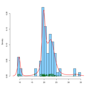
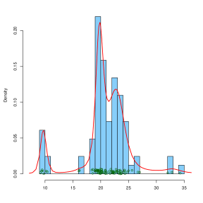
In this section, we look at the performance of iIS and iWAIC in approximating CVIC of fitting finite mixture models to Galaxy data (Postman et al., 1986; Roeder, 1990) which is used very often to demonstrate mixture modelling methods. We obtained the data set from R package MASS. The data set is a numeric vector of velocities (km/sec) of 82 galaxies from 6 well-separated conic sections of an unfilled survey of the Corona Borealis region. We applied mixture modelling to the velocities divided by 1000. A histogram of these 82 numbers is shown in each plot of Figure 2, which also shows three fitted density functions to be discussed later. Our purpose of computing CVIC for finite mixture models is to determine the numbers of mixture components, , that can adequately capture the heterogeneity in a data but don’t overfit the data. The finite mixture model that we used to fit Galaxy data is as follows:
| (28) | |||||
| (29) | |||||
| (30) | |||||
| (31) | |||||
| (32) |
Here we set the prior mean of to 20, which is the mean of the 82 numbers, and set the scale for Inverse Gamma prior for to 20, which is the variance of the 82 numbers.

The finite mixture model (equations (28) - (32)) falls in the class of models depicted by Figure 1: the observed variable is , the model parameters is , and the latent variable is mixture component indicator . In this model, the latent variables are independent given the model parameter . It follows that are independent given .
We used JAGS (Plummer, 2003) to run MCMC simulations for fitting the above model to Galaxy data with various choice of . To avoid the problem that MCMC may get stuck in a model with only one component, we followed JAGS eyes example to restrict the MCMC to have at least a data point in each component. All MCMC simulations started with a randomly generated , and ran 5 parallel chains, each doing 2000, 2000, and 100,000 iterations for adapting, burning, and sampling, respectively.
We ran actual 82 cross-validatory MCMC simulations with each of the 82 numbers removed (set to NA in JAGS). After each simulation, we computed actual CV posterior predictive density using equation (5) with evaluation function set to , where represents normal density. Using all 82 values of CV posterior predictive densities, we can compute CVIC using equation (7). The CVICs for different choices of based on one simulation for each are displayed in Table 1. We repeated computing CVICs quite a few times, and the results were almost the same, with only differences in the 2nd decimal.
We then considered approximating CVIC using four different methods (nIS, nWAIC, iIS, iWAIC) from a single MCMC simulation that is based on all of the 82 numbers. The non-integrated predictive density for this model is as specified in (28); this is normal density with mean and standard deviation , denoted by . The values of computed with a collection of MCMC samples of are then used for computing nIS and nWAIC approximates of CV posterior predictive densities (with equations (13) and (24) respectively). We can then compute nIS information criterion and nWAIC by plugging the approximates of CV posterior predictive densities into (7). The integrated predictive density is ( note that and are independent given ). We can then use for computing iIS and iWAIC approximates of CV posterior predictive densities (with equations (21) and (26) respectively), and corresponding information criterion values. In this example, iIS and iWAIC are just applications of IS and WAIC to mixture models with latent variables integrated out.
| DIC | nWAIC | nIS | iWAIC | iIS | CVIC | |
|---|---|---|---|---|---|---|
| 2 | 445.38(1.64) | 420.27(0.39) | 425.63(3.45) | 449.56(0.14) | 449.62(0.17) | 450.55 |
| 3 | 528.78(45.12) | 384.94(9.94) | 391.29(6.17) | 437.23(4.70) | 436.43(3.79) | 427.46 |
| 4 | 774.85(31.58) | 339.91(1.87) | 363.55(5.32) | 422.43(0.53) | 422.76(0.54) | 423.16 |
| 5 | 710.88(25.34) | 328.19(0.29) | 362.30(3.70) | 421.02(0.09) | 421.41(0.10) | 421.10 |
| 6 | 679.95(17.48) | 323.62(1.33) | 355.49(5.72) | 420.97(0.27) | 421.35(0.31) | 421.34 |
| 7 | 675.27(18.57) | 321.61(0.30) | 364.41(4.49) | 421.25(0.07) | 421.64(0.12) | 421.53 |
For each choice of , we computed the above four criteria as well as DIC (using R package R2jags) for 100 independent MCMC simulations. Table 1 shows the means of these 100 information criterion values for each approximation method, with standard deviations shown in brackets. From the table, we see that the naive applications of WAIC and IS to non-integrated predictive densities do not work satisfactorily. They are both highly downward biased. Furthermore, nWAIC chooses over-complex models because nWAICs keep decreasing until , and nIS estimates of CVIC have very high variances. DICs for this example turn into a mess because the model parameters are non-identifiable. iIS and iWAIC provide significantly closer estimates of actual CVIC, with much smaller standard deviations, than other methods. These results show that using integrated predictive densities significantly improves accuracy of nIS and nWAIC. The results of iWAIC may not be surprising because here iWAIC is just application of WAIC to the marginalized models with latent variables integrated out, in which observed variables are independent given model parameters. Watanabe (2010a) has proven the asymptotic equivalence of WAIC and CVIC in such models. iIS is also theoretically justified in Section 4.
| pair of models | nWAIC | nIS | iWAIC | iIS | CVIC |
|---|---|---|---|---|---|
| 3 vs 2 | 0.000 | 0.000 | 0.016 | 0.013 | 0.010 |
| 4 vs 3 | 0.000 | 0.019 | 0.030 | 0.032 | 0.190 |
| 5 vs 4 | 0.000 | 0.249 | 0.070 | 0.066 | 0.027 |
| 6 vs 5 | 0.002 | 0.203 | 0.489 | 0.476 | 0.674 |
| 7 vs 6 | 0.110 | 0.840 | 0.716 | 0.711 | 0.700 |
CVIC is the sum of minus twice of log CV posterior predictive densities. Therefore, the statistical significance of the differences of two CVICs (or estimates) can be accessed by looking at the population mean differences of two groups of log CV posterior predictive densities (Vehtari, 2001; Vehtari and Lampinen, 2002). We conducted one-sided paired t-test to test whether a finite mixture model with components provides a better fit (larger mean of CV posterior predictive densities) to Galaxy data than a mixture model with components. The p-values of the comparisons for for actual CV posterior predictive densities are given in Table 2 (column CVIC). We also conducted the same test for log CV posterior predictive densities estimated by four different methods (nIS, iIS, nWAIC, iWAIC). Due to the variations in these estimates, we computed the p-values 1000 times by randomly drawing two simulation results from models with and components. We then computed the mean of the 1000 p-values. Table 2 shows the results for all four different estimation methods. From the table, we see that iIS and iWAIC provides much closer p-values to those based on actual CV posterior predictive densities than nIS and nWAIC. These p-values indicates that mixture models with 5 components are adequate to capture the heterogeneity in Galaxy data, and 6-component mixture models does not provide better fit with statistical significance. These conclusions can be visualized by the density curves given by fitting resulting with , where the curves with and are different, but the curves with and are almost the same.
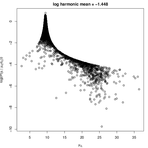
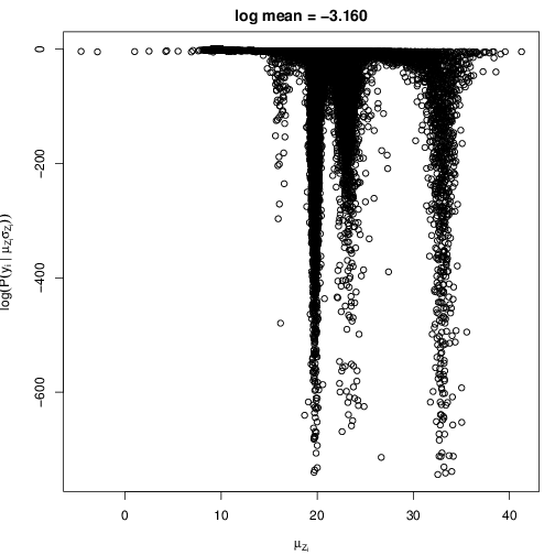
Last, we explain why naive applications of IS and WAIC to non-integrated predictive densities cannot provide good estimates of CV posterior predictive densities. Figure 3 show scatter-plots of the log non-integrated predictive density, , against , computed with each MCMC sample of from the full data posterior (Figure (3a)) and the actual CV posterior with the removed (Figure (3b)), where is the 3rd of the 82 numbers. From the figure, we see great discrepancy between the posterior distribution of the non-integrated predictive density with and without included in MCMC simulations. When we simulate MCMC with the full data ( included), most of the visit components that fit well, with most of are around 10. Thus, the non-integrated predictive densities are mostly very high. When we simulate MCMC with removed, most of the visit large components, hence the visits much more often the interval from 10 to 35 that do not fit well. The reason is that without the inclusion of , the will more likely take larger components. Thus, values of in the CV posterior are very low, with greatly lower order in magnitude than in the full data posterior. This indicates that the difference between the CV posterior and full data posterior of is huge. Applying IS and WAIC to the non-integrated predictive densities alone is unable to correct for much of the bias due to the inclusion of in MCMC simulation. By averaging the non-integrated predictive density over regenerated given but not , we significantly reduce the optimistic bias in ) due to inclusion of . This explains why iIS and iWAIC provide significantly closer estimates to CVIC than nIS and nWAIC.
6.2 A Simulation Study with Finite Mixture Models
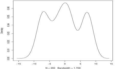
In this section, we report a simulation study with the same mixture models described in Section 6.1. We simulated 100 data sets, each containing 200 data points from a mixture distribution with normal components: . The kernel density of one of the data sets are shown in Figure 4. From this plot, we see that the middle two components may be hard to separate in some data sets.
We fitted each of the 100 data sets using the exactly same way described in Section 6.1, and then computed information criterion (IC) using each of the five methods (nWAIC, nIS, iWAIC, iIS and DIC). Table 3 show the IC values for two selected data sets. Table (4a) shows averages of IC values in 100 data sets, for each model indexed by (row) and for each method for approximating CVIC (column). Table (4b) shows frequencies of selected models in 100 data sets by looking at the minimum IC value computed with each of the five methods (column).
| nWAIC | nIS | iWAIC | iIS | DIC | |
|---|---|---|---|---|---|
| 2 | 1022.95 | 1081.11 | 1163.96 | 1163.99 | 1143.19 |
| 3 | 690.39 | 855.85 | 1088.20 | 1088.26 | 850.28 |
| 4 | 642.82 | 782.94 | 1083.16 | 1083.28 | 1416.81 |
| 5 | 640.27 | 754.13 | 1084.29 | 1084.48 | 1351.18 |
| 6 | 638.25 | 756.82 | 1085.25 | 1085.51 | 1382.83 |
| 7 | 637.12 | 727.84 | 1086.46 | 1086.76 | 1479.03 |
| nWAIC | nIS | iWAIC | iIS | DIC | |
|---|---|---|---|---|---|
| 2 | 1144.14 | 1122.07 | 1202.25 | 1199.90 | 1192.42 |
| 3 | 758.35 | 924.19 | 1101.48 | 1101.53 | 1024.83 |
| 4 | 706.30 | 830.63 | 1095.42 | 1095.54 | 1510.18 |
| 5 | 691.02 | 821.51 | 1094.84 | 1094.99 | 1561.51 |
| 6 | 679.71 | 800.38 | 1094.64 | 1094.80 | 1652.05 |
| 7 | 673.63 | 794.05 | 1094.69 | 1094.87 | 1740.80 |
| nIS | nWAIC | iIS | iWAIC | DIC | |
|---|---|---|---|---|---|
| 2 | 1112.48 | 1103.95 | 1181.60 | 1182.33 | 1248.97 |
| 3 | 922.88 | 751.58 | 1105.18 | 1105.11 | 990.51 |
| 4 | 827.06 | 682.62 | 1099.42 | 1099.26 | 1572.80 |
| 5 | 810.42 | 674.39 | 1099.18 | 1098.96 | 1562.05 |
| 6 | 801.24 | 669.57 | 1099.60 | 1099.31 | 1630.02 |
| 7 | 796.65 | 666.39 | 1100.09 | 1099.77 | 1700.12 |
| nIS | nWAIC | iIS | iWAIC | DIC | |
|---|---|---|---|---|---|
| 2 | 0 | 0 | 0 | 0 | 2 |
| 3 | 0 | 0 | 15 | 15 | 94 |
| 4 | 6 | 15 | 39 | 37 | 4 |
| 5 | 10 | 4 | 21 | 20 | 0 |
| 6 | 30 | 8 | 11 | 13 | 0 |
| 7 | 54 | 73 | 14 | 15 | 0 |
In both of the data sets shown in Table 3, nWAIC and nIS select the model with , which is more flexible than the true data generating model, which has . This is typical for the 100 data sets, which can be seen from Tables (4a) and (4b). DIC, on the other hand, almost always selects the model with which is simpler than the true model (). These results are consistent with what we observe from the analysis of Galaxy data. For iWAIC and iIS, their IC values have a sharp decrease from until , compared to the changes in the IC values after , which stabilize and have only very small variation. This small variation sometimes leads to wrong model selection results if one chooses the model with the smallest IC value, for example in the data set shown by Table (3b). Therefore, IC may not be sensitive enough in penalizing over-complex models. Overall, in this example, iWAIC and iIS outperform nWAIC, nIS and DIC in comparing models because of the improved estimation of CVIC. With IC values computed by iWAIC and iIS, the appropriate decision () can be made for most data sets if one does not simply look at which model has the smallest IC value but also the change of IC values in all models considered.
In this example, IC cannot penalize over-complex models sensitively. The insensitivity occurs because the posterior inference with MCMC itself is robust to over-complexity in models, that is, MCMC simulation can automatically adjust the model complexity. For example, in this example, although we fit a mixture model with components, some components have very small proportions in MCMC samples, which is effectively a simpler model. This has been long known as a good property for Bayesian inference, see extensive discussions by Neal (1995). However, this poses difficulty in model selection by looking at CVIC. We’ve noticed that recently Wang and Gelman (2014) have also discussed the insensitivity of CVIC. They explain the insensitive as that the the criterion CVIC itself is not sensitive in distinguishing models for binary data. Overall, how to determine a threshold for CVIC (even computed with actual cross-validation) for selecting models, particularly among models with slight difference, is still a problem, which demands further study. Looking at the population mean of log CV posterior predictive density may be an option, as we discuss in Galaxy data analysis results. However, we feel that generally this may be too conservative because a model is better than another not because it can provides better predictive accuracy for “most” observations (resulting in a sharp change in population mean — CVIC), but rather it can provide better prediction only for a fraction of observations. Perhaps, we should look at the proportion of units whose predictions have been improved with a more complex model.
6.3 Random Spatial Effect Models for Scottish Lip Cancer Data
In this section, we investigated the performance of iIS and iWAIC in an analysis of Scottish lip cancer data, which was used in Stern and Cressie (2000); Spiegelhalter et al. (2002); Plummer (2008). The data set was extracted from the paper by Stern and Cressie (2000). The data represents male lip cancer counts (over the period 1975 - 1980) in the districts of Scotland. At each district , the data include these fields: (1) the number of observed cases of lip cancer, ; (2) the number of expected cases, , calculated based on standardization of “population at risk” across different age groups; (3) the percent of population employed in agriculture, fishing and forestry, , used as a covariate; and (4) a list of the neighbouring regions.
The , for , is modelled as an independent Poisson random variable conditional on and :
| (33) |
where denotes the underlying relative risk for district , and stands for expected counts. Let and . We consider four different models for the vector conditional on and neighbouring information between districts:
| (34) | |||
| (35) | |||
| (36) | |||
| (37) |
where is a matrix for capturing the spatial correlations amongst the districts, in which, the elements of are: if areas and are neighbours, and 0 otherwise; the elements of are: and if . The multivariate normal distributions with as covariance matrix are called proper conditional auto-regression (CAR) model. Derived from the joint distribution in (34), the conditional distribution of is:
| (38) |
where is the set of neighbours of district . From (38), we see that controls the degree of spatial dependency of on its neighbours. At a higher level, diffused priors are assigned to , and : where is the interval for such that is positive-definite (see Stern and Cressie, 2000). In model (34), we consider both spatial and linear effects of in modelling . One may also consider other models. Model (35) considers only spatial effect; model (36) considers only linear effect; and model (37) considers none of spatial and linear effect. We are interested in comparing goodness-of-fits of the four models to lip cancer data set so as to determine which model is the most appropriate for Scottish lip cancer data. CVIC is one criterion for measuring goodness-of-fit.
All the above four models belong to the class of Bayesian latent variable models depicted by Figure 1. The observable variable is , the latent variable is , and the model parameters in model (34) are , and a subset of it for other models depending on which are used in respective models. We used OpenBUGS through R package R2OpenBUGS to run MCMC simulations for fitting each of the above models to Scottish lip cancer data. For each simulation, we ran two parrallel chains, each with 15000 iterations, and the first 5000 were discarded as burn-in.
For each model, we first ran actual 56 cross-validatory MCMC simulations with each of the 56 obervations removed (set to NA in OpenBUGS) and then computed actual CV posterior predictive density using equation (5) with evaluation function set to — Poisson probability mass function with parameter . Then we computed CVIC using equation (7). We computed actual CVIC 10 times for each model although actual LOOCV gives very stable results. The averages and standard deviations of 10 CVICs for different models are displayed in Table 5. From this table, we see that the spatial+linear model is optimal for the Scottish lip cancer data according to CVIC.
We then consider approximating CVIC with four different methods (nIS, nWAIC, iIS, and iWAIC) from a single MCMC simulation based on all of the 56 observations. The non-integrated predictive density used in computing nIS and nWAIC with equations (13) and (24) is , where . Next, we describe how to compute iIS and iWAIC for model (34). The integrated predictive density (18) required by (21) and (26) is:
| (39) |
where is given by equation (38). Because there is no closed form for the integral (39), we use Monte Carlo method to estimate it by generating 200 random numbers from (note, this is done for each retained MCMC sample of and each validation unit , with alternately discarded). Finally, based on computed values of for all MCMC samples, we can then compute iIS and iWAIC approximates of CV posterior predictive densities (with equations (21) and (26) respectively) and then corresponding iIS information criterion and iWAIC. iIS and iWAIC are computed similarly for models (35) - (37), with only a change of the conditional distribution (38) according to their joint prior distributions.
We repeated computing the values of the above four criteria as well as DIC for 100 independent MCMC simulations based on each model. The means of these 100 information criterion values for each method and each model are shown in Table 5, with standard deviations shown in brackets. We see that, iIS and iWAIC provide significantly closer approximates to actual CVIC than nIS, nWAIC and DIC; furthermore, the approximates by iWAIC and iIS are almost identical to actual CVIC. In contrast, DIC has large biases and variances when spatial effects are considered, and also the mean DIC of the spatial + linear model is bigger than the mean DIC of the model with spatial effects only. This suggests that, if we randomly draw one MCMC simulation out of the 100 ones based on each model, the probability that DIC does NOT pick up the spatial+linear model as the optimal model is high (56.6% if we assume the DICs are normally distributed). nWAIC and nIS also have large biases and variances. In particular, nWAIC nearly never chooses the spatial+linear model (with a probability close to 1 if nWAICs are normally distributed). nIS has a good chance (0.92 if the values are normally distribute) to choose the spatial+linear model. However, nIS is numerically unstable, with fairly large variance, which has been well-known to many people (Spiegelhalter et al., 2002). In summary, the integration applied to latent variables associated with each validation unit substantially improve the estimates of CVIC given by nWAIC and nIS.
| DIC | nWAIC | nIS | iWAIC | iIS | CVIC | |
|---|---|---|---|---|---|---|
| spa.+lin. | 269.43(12.30) | 306.82(0.21) | 335.54(1.27) | 344.47(0.12) | 345.21(0.19) | 343.88(0.14) |
| spatial | 266.79(10.15) | 304.61(0.18) | 338.77(1.85) | 354.11(0.06) | 356.06(0.37) | 352.54(0.14) |
| linear | 310.42(0.11) | 306.94(0.21) | 338.81(3.02) | 350.48(0.05) | 350.54(0.05) | 349.48(0.11) |
| exch. | 312.57(0.12) | 306.74(0.17) | 346.55(3.46) | 368.01(0.03) | 368.08(0.03) | 366.61(0.00) |
The good approximations of CVIC by iIS may not be surprising, because our derivation in Section 4.2 has shown their equivalence in these models. It is surprising to note that the heuristic iWAIC also gives estimates very close to CVIC for model (34) and (35), which contain actually correlated random effects. Furthermore, note that iWAIC has smaller standard deviations and biases than iIS. Therefore, the equivalence of iWAIC to iIS (or CVIC) deserves more empirical and theoretical investigations in the future.
6.4 CV Posterior p-values in Logistic Regression for Seeds Data
We consider comparing different methods for computing posterior p-values for identifying outliers in applying logistic regression with random effects to Seeds data, a classic example of WinBUGS (http://www.mrc-bsu.cam.ac.uk/bugs/winbugs/Vol1.pdf). We obtained the data set from the previous link. The example is taken from Table 3 of Crowder (1978). The study concerns about the proportion of seeds that germinated on each of 21 plates arranged according to a 2 by 2 factorial layout by seed and type of root extract. For , let be the number of germinated seeds in the th plate, be the total number of seeds in the th plate, be the seed type (0/1), and be root extract (0/1). The conditional distribution of given , and are specified as follows:
| (40) | |||||
| (41) | |||||
| (42) |
and parameters are assigned with as prior, and is assigned with Inverse-Gamma (0.001, 0.001) as prior. The above model is a member of Bayesian latent variable models depicted by Figure 1. The observable variable is , the latent variable is , the covariate variable vector is , and the model parameter vector is . We used JAGS to run MCMC for fitting the above model to the Seeds data. For each simulation, we ran 5 parallel chains, each running 1000 iterations for adapting, 2500 iterations for burning in, and 10000 iterations for sampling.
The p-value (given parameters and latent variable) defined by (8) for this example is the right tail probability of Binomial distribution with number of trials and success rate :
| (43) |
where is the actual observation of , and pbinom and dbinom denote CDF and PMF of Binomial distribution. Very small or very large p-values indicate that the actual observed falls on the tails of (ie, is unusual to) Binomial (, ). CV posterior p-value (Marshall and Spiegelhalter, 2003) for observation is the mean of with respect to the CV posterior distribution . If we get a very small or very large CV posterior p-value for observation , it indicates that is unusual to the predictive distribution of given . For this example, when CV posterior p-value for is very small or very large, the germination rate, , of the th plate is probably an outlier to other plates. Marshall and Spiegelhalter (2007) showed that the CV posterior p-values are uniformly distributed on interval . We ran actual CV MCMC simulations to find the CV posterior p-values for each of the 21 plates, and the results are displayed by the x-axis in plots of Figure 5.
We compared four different methods for computing posterior p-values for identifying outliers with only a single MCMC simulation based on the full data set. One method is to apply posterior checking idea of Gelman et al. (1996) without considering bias-correction, that is, to average each p-value with respect to the posterior of given the full data set . We will call this method by posterior checking. Gelman et al. (1996) do not recommend this use of posterior checking because it uses data twice in model building and assessment. However, this method is convenient and so perhaps used very often in practice. Therefore, we include it in comparison. To reduce the bias of including in model fitting, Marshall and Spiegelhalter (2003) propose ghosting method: for each MCMC sample, one averages p-value with respect to the conditional distribution of given (but without ) to obtain ghosting p-value (which can be done with Monte carlo method by re-generating given with no reference to ), then averages the ghosting p-values over all MCMC samples. The third method is non-integrated importance sampling method (nIS) that averages p-value after being weighted with the inverse of probability density (mass) of : . The fourth method is integrated importance sampling (iIS). For each MCMC sample, we first average both p-value and with respect to to find the integrated evaluation p-value (equation (47)) and the integrated predictive density (equation (18)) respectively, then compute the weighted average of the integrated p-values with the reversed integrated predictive density as weights over all MCMC samples using formula (19). We can see that the way to obtain ghosting p-value is the same as finding integrated p-value in (47) when are independent given , but without using the reversed integrated density to correct for the optimistic bias in full data posterior of parameters. Therefore, ghosting method can be viewed as a partial implementation of iIS method presented here.
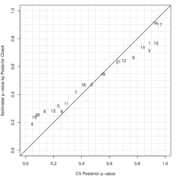
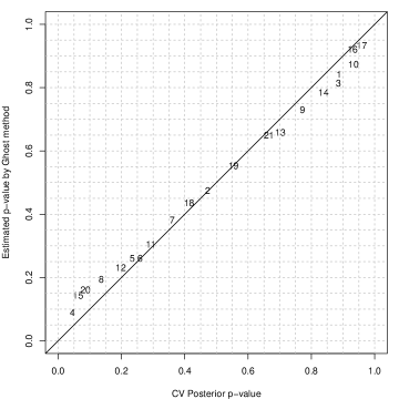
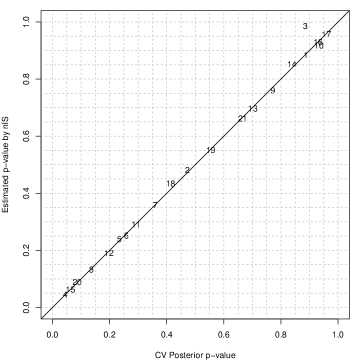

We calculated 21 posterior p-values with the four method given a MCMC simulation based on the full data set, and repeated this calculation for 100 independent MCMC simulations. For computing integrated p-values and predictive densities as needed by nIS and ghosting method, we generated 30 of from for each plate and each MCMC sample. Figure 5 shows the scatter-plots of four sets of estimated posterior p-values given by four different methods against the actual CV posterior p-values from one MCMC simulation. From the figure, we see that the p-values given by posterior checking are more concentrated around 0.5 than the actual CV posterior p-values, and do not appear to be uniformly distributed (Gelman, 2013). This is because in computing each p-value, the observed value itself is included in model fitting, resulting in optimistic bias. Ghosting method reduces the bias, hence the estimated p-values are closer to the actual CV p-values, and more spread out over . However, for this example, the bias is still visible from Figure (5b). Both nIS and iIS give estimates that are very close to the actual values found by CV. However, nIS is less stable than iIS, and sometimes gives very poor estimates; for example the 3rd plate shown in Figure (5c).
To measure more precisely the accuracy of estimated p-values to the actual CV p-values, we use absolute relative error in percentage scale defined as
| (44) |
where are estimates of . This measure emphasizes greatly on the error between and when is very small or very large, for which we demand more on absolute error than when is close to 0.5. A similar measure (only using in denominator) is used by Marshall and Spiegelhalter (2007). Here we modify the denominator because large p-values are important too. Table 6 shows the averages of REs over 100 independent simulations for each method. Clearly, we see that iIS is the best among the four, and improve significantly ghosting and posterior checking methods.
| iIS | nIS | Ghosting | Posterior checking |
| 2.319(0.399) | 5.234(1.083) | 35.610(1.267) | 93.887(3.854) |
7 Conclusions and Discussions
In this article, we have introduced two methods (iIS and iWAIC) for approximating leave-one-out cross-validatory predictive evaluations for models with unit-specific and possibly correlated latent variables. The innovation in iIS and iWAIC is that we replace the non-integrated predictive density and evaluation functions by the integrated predictive density and evaluation functions. iIS is applicable to models with non-identifiable parametrization for which DIC may not be suitable; and also applicable to models with correlated latent variables for which WAIC is not. The extent of applicability of iWAIC remains to be investigated. We have tested iIS and iWAIC in four examples, in which iIS and/or iWAIC provide almost identical approximates to what given by actual leave-one-out cross-validation, whereas other methods show large discrepancies. In addition, we have found that iWAIC is slightly more stable than iIS.
Although our empirical results show that iIS and iWAIC provide better approximates of CVIC than DIC, we notice that the implementations of iIS and iWAIC are much more complicated, and requires users to have basic knowledge in statistics and scientific computing (for example a degree in statistics). For the moment, we do not know how to automate their applications as DIC, which can be embedded into a black-box MCMC sampler program. This is a direction for future research one can pursue.
Applicability of iWAIC to models with correlated latent variables still requires more empirical and theoretical investigations. The results of our empirical studies in the lip cancer data give an example that iWAIC provides very close approximates to CVIC. However, we have to be cautious in the generalization of iWAIC to other models and problems. In the future, we will empirically test iWAIC in many other models using correlated latent variables, for example, the stochastic volatility models used for modelling financial time sequences (Jacquier et al., 2002; Gander and Stephens, 2007), multivariate spatial models (Feng and Dean, 2012), and many other models considering spatial and temporal correlations (Waller et al., 1997). We will also investigate iWAIC theoretically, probably using the tools for singular statistical models developed by Watanabe (2009).
There is also much research work needed to generalize and extend iIS and iWAIC. We have only shown how to integrate latent variables away in the models where they are unit-specific to improve ordinary nIS and nWAIC. In many models, a latent variable is shared by many observations. It is still unclear to us how to improve nIS and nWAIC in such models. More ambitiously, we may wonder whether there is a method that requires little technical work but provides very good predictive evaluation for all Bayesian models.
The insensitivity of CVIC is another important problem that demands further research, as we discuss in Section 6.2. One may consider other evaluation function than log predictive density for capturing sensitively the difference among models. One may also consider other methods for comparing two sets of log predictive densities resulting from two competing models. However, we think that the method we present in this article for latent variable models may be generally useful for providing better approximation of cross-validatory quantities regardless of the choice of evaluation function.
Appendices
Appendix A Working procedure of iIS
-
1.
Generate MCMC samples ; s= 1,…,S} from
-
2.
For each
-
(a)
For each , generate from , and estimate by
(45) Then, we can find iIS weight:
(46) -
(b)
For each , generate from , and estimate integrated evaluation function by
(47)
-
(a)
-
3.
Estimate expected evaluation function with respect to by
(48)
Note that, if we are only interested in computing CVIC, don’t need to do step 2(b), and take the numerator in (48) to be 1 as warranted by theory.
Appendix B Working procedure of iWAIC
-
1.
Generate MCMC samples ; s= 1,…,S} from
-
2.
For each and each , generate from , and estimate integrated predictive density by
(49) -
3.
Estimate log CV posterior predictive density:
(50) where stands for sample variance of ).
-
4.
Find iWAIC:
(51)
References
- Ando (2007) Ando, T. (2007), “Bayesian predictive information criterion for the evaluation of hierarchical Bayesian and empirical Bayes models,” Biometrika, 94, 443–458.
- Berger and Pericchi (1996) Berger, J. O. and Pericchi, L. R. (1996), “The intrinsic Bayes factor for model selection and prediction,” Journal of the American Statistical Association, 91, 109–122.
- Bernardo and Rueda (2002) Bernardo, J. M. and Rueda, R. (2002), “Bayesian hypothesis testing: A reference approach,” International Statistical Review, 70, 351–372.
- Bhattacharya and Haslett (2007) Bhattacharya, S. and Haslett, J. (2007), “Importance re-sampling MCMC for cross-validation in inverse problems,” Bayesian Analysis, 2, 385–407.
- Celeux et al. (2006) Celeux, G., Forbes, F., Robert, C. P., and Titterington, D. M. (2006), “Deviance information criteria for missing data models,” Bayesian Analysis, 1, 651–673.
- Chib (1995) Chib, S. (1995), “Marginal Likelihood from the Gibbs Output,” JASA, 1313–1321.
- Crowder (1978) Crowder, M. J. (1978), “Beta-binomial Anova for proportions,” Applied Statistics, 27, 34–37.
- Epifani et al. (2008) Epifani, I., MacEachern, S. N., and Peruggia, M. (2008), “Case-deletion importance sampling estimators: Central limit theorems and related results,” Electronic Journal of Statistics, 2, 774–806.
- Feng and Dean (2012) Feng, C. and Dean, C. (2012), “Joint analysis of multivariate spatial count and zero-heavy count outcomes using common spatial factor models,” Environmetrics, 23, 493–508.
- Gander and Stephens (2007) Gander, M. P. and Stephens, D. A. (2007), “Stochastic volatility modelling in continuous time with general marginal distributions: Inference, prediction and model selection,” JSPI, 137, 3068–3081.
- Gelfand et al. (1992) Gelfand, A. E., Dey, D. K., and Chang, H. (1992), “Model Determination using Predictive Distributions with Implementation via Sampling-Based Methods (with discussion),” in Bayesian Statistics 4, pp. 147–167.
- Gelman (2013) Gelman, A. (2013), “Understanding posterior p-values,” unpublished online manuscript, available from Gelman’s website., 1–8.
- Gelman et al. (2014) Gelman, A., Hwang, J., and Vehtari, A. (2014), “Understanding predictive information criteria for Bayesian models,” Statistics and Computing, 24, 997–1016.
- Gelman and Meng (1998) Gelman, A. and Meng, X. (1998), “Simulating normalizing constants: From importance sampling to bridge sampling to path sampling,” Statistical Science, 163–185.
- Gelman et al. (1996) Gelman, A., Meng, X., and Stern, H. (1996), “Posterior predictive assessment of model fitness via realized discrepancies,” Statistica Sinica, 6, 733–760.
- Geweke (1989) Geweke, J. (1989), “Bayesian inference in econometric models using Monte Carlo integration,” Econometrica: Journal of the Econometric Society, 1317–1339.
- Hachiya et al. (2008) Hachiya, H., Akiyama, T., Sugiyama, M., and Peters, J. (2008), “Adaptive Importance Sampling with Automatic Model Selection in Value Function Approximation.” pp. 1351–1356.
- Held et al. (2010) Held, L., Schrödle, B., and Rue, H. (2010), “Posterior and Cross-validatory Predictive Checks: A Comparison of MCMC and INLA,” in Statistical Modelling and Regression Structures, eds. Kneib, T. and Tutz, G., Physica-Verlag HD, pp. 91–110.
- Jacquier et al. (2002) Jacquier, E., Polson, N. G., and Rossi, P. E. (2002), “Bayesian analysis of stochastic volatility models,” Journal of Business & Economic Statistics, 20, 69–87.
- Kass and Raftery (1995) Kass, R. E. and Raftery, A. E. (1995), “Bayes Factors,” Journal of the American Statistical Association, 90, 773–795.
- Li and Yu (2012) Li, Y. and Yu, J. (2012), “Bayesian hypothesis testing in latent variable models,” Journal of Econometrics, 166, 237–246.
- Li et al. (2012) Li, Y., Zeng, T., and Yu, J. (2012), “Robust deviance information criterion for latent variable models,” .
- Li et al. (2014) — (2014), “A new approach to Bayesian hypothesis testing,” Journal of Econometrics, 178, 602–612.
- Lindley (1957) Lindley, D. V. (1957), “A statistical paradox,” Biometrika, 44, 187–187.
- Liu (2001) Liu, J. S. (2001), Monte Carlo Strategies in Scientific Computing, Springer-Verlag.
- Marshall and Spiegelhalter (2003) Marshall, E. C. and Spiegelhalter, D. J. (2003), “Approximate cross-validatory predictive checks in disease mapping models,” Stat. Med., 22, 1649–1660.
- Marshall and Spiegelhalter (2007) — (2007), “Identifying outliers in Bayesian hierarchical models: a simulation-based approach,” Bayesian Analysis, 2, 409–444.
- Neal (1993) Neal, R. M. (1993), “Probabilistic Inference using Markov Chain Monte Carlo Methods,” Tech. rep., Dept. of Computer Science, University of Toronto.
- Neal (1995) — (1995), “Bayesian learning for neural networks,” Ph.D. thesis, University of Toronto.
- O’Hagan (1995) O’Hagan, A. (1995), “Fractional Bayes factors for model comparison,” Journal of the Royal Statistical Society. Series B (Methodological), 99–138.
- O’Hagan (1997) — (1997), “Properties of intrinsic and fractional Bayes factors,” Test, 6, 101–118.
- Peruggia (1997) Peruggia, M. (1997), “On the variability of case-deletion Importance sampling Weights in the Bayesian linear model,” JASA, 92, 199–207.
- Plummer (2003) Plummer, M. (2003), “JAGS: A program for analysis of Bayesian graphical models using Gibbs sampling,” in Proceedings of the 3rd International Workshop on Distributed Statistical Computing (DSC 2003). March, pp. 20–22.
- Plummer (2008) — (2008), “Penalized loss functions for Bayesian model comparison,” Biostatistics, 9, 523–539.
- Postman et al. (1986) Postman, M., Huchra, J. P., and Geller, M. J. (1986), “Probes of large-scale structure in the Corona Borealis region,” The Astronomical Journal, 92, 1238–1247.
- Raftery et al. (2006) Raftery, A. E., Newton, M. A., Satagopan, J. M., and Krivitsky, P. N. (2006), “Estimating the integrated likelihood via posterior simulation using the harmonic mean identity,” .
- Robert (2013) Robert, C. P. (2013), “On the Jeffreys-Lindley’s paradox,” ArXiv, 1303.5973v, 1–13.
- Roeder (1990) Roeder, K. (1990), “Density estimation with confidence sets exemplified by superclusters and voids in the galaxies,” JASA, 85, 617–624.
- Spiegelhalter et al. (2002) Spiegelhalter, D. J., Best, N. G., Carlin, B. P., and van der Linde, A. (2002), “Bayesian measures of model complexity and fit,” JRSSB, 64, 583–639.
- Stern and Cressie (2000) Stern, H. S. and Cressie, N. (2000), “Posterior predictive model checks for disease mapping models,” Statistics in medicine, 19, 2377–2397.
- Vanhatalo et al. (2012) Vanhatalo, J., Riihimäki, J., Hartikainen, J., Jylänki, P., Tolvanen, V., and Vehtari, A. (2012), “Bayesian Modeling with Gaussian Processes using the GPstuff Toolbox,” arXiv:1206.5754 [cs, stat].
- Vanhatalo et al. (2013) — (2013), “GPstuff: Bayesian modeling with Gaussian processes,” The Journal of Machine Learning Research, 14, 1175–1179.
- Vehtari (2001) Vehtari, A. (2001), “Bayesian model assessment and selection using expected utilities,” Ph.D. thesis, HELSINKI UNIVERSITY OF TECHNOLOGY.
- Vehtari and Lampinen (2002) Vehtari, A. and Lampinen, J. (2002), “Bayesian model assessment and comparison using cross-validation predictive densities,” Neural Comput., 14, 2439–2468.
- Vehtari and Ojanen (2012) Vehtari, A. and Ojanen, J. (2012), “A survey of Bayesian predictive methods for model assessment, selection and comparison,” Statistics Surveys, 6, 142–228.
- Waller et al. (1997) Waller, L. A., Carlin, B. P., Xia, H., and Gelfand, A. E. (1997), “Hierarchical Spatio-Temporal Mapping of Disease Rates,” JASA, 92, 607–617.
- Wang and Gelman (2014) Wang, W. and Gelman, A. (2014), “Difficulty of selecting among multilevel models using predictive accuracy,” .
- Watanabe (2009) Watanabe, S. (2009), Algebraic geometry and statistical learning theory, Cambridge University Press.
- Watanabe (2010a) — (2010a), “Asymptotic Equivalence of Bayes Cross Validation and Widely Applicable Information Criterion in Singular Learning Theory,” Journal of Machine Learning Research, 11, 3571–3594.
- Watanabe (2010b) — (2010b), “Equations of states in singular statistical estimation,” Neural Networks, 23, 20–34.
- Watanabe (2010c) — (2010c), “Equations of states in statistical learning for an unrealizable and regular case,” IEICE transactions on fundamentals of electronics, communications and computer sciences, 93, 617–626.