Memory effects in biochemical networks as the natural counterpart of extrinsic noise

Abstract

We show that in the generic situation where a biological network, e.g. a protein interaction network, is in fact a subnetwork embedded in a larger “bulk” network, the presence of the bulk causes not just extrinsic noise but also memory effects. This means that the dynamics of the subnetwork will depend not only on its present state, but also its past. We use projection techniques to get explicit expressions for the memory functions that encode such memory effects, for generic protein interaction networks involving binary and unary reactions such as complex formation and phosphorylation, respectively. Remarkably, in the limit of low intrinsic copy-number noise such expressions can be obtained even for nonlinear dependences on the past. We illustrate the method with examples from a protein interaction network around epidermal growth factor receptor (EGFR), which is relevant to cancer signalling. These examples demonstrate that inclusion of memory terms is not only important conceptually but also leads to substantially higher quantitative accuracy in the predicted subnetwork dynamics.

1 Introduction

Biological networks are often complex and models are required to try and understand their behaviour [1]. This has stimulated an ongoing research effort into the construction of reduced models that allow one to focus on subnetworks of a larger system. Such subnetworks may carry out biologically important functions, or be of interest because they capture parts of the system where there is less uncertainty in the network structure or dynamical parameters such as reaction rates. The example network considered here is epidermal growth factor receptor (EGFR) signalling, which is a relatively small and well-studied network [2] and contains a number of subnetworks, such as Src homology and collagen domain protein (Shc) and Shc-interacting proteins. An understanding of the properties of such subnetworks can then in turn be used to help rationalise the behaviour of a larger network [3, 4, 5].

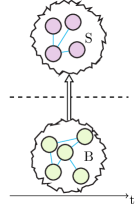
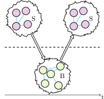
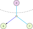
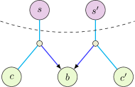
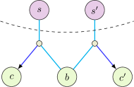
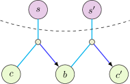
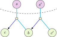
The above considerations motivate the analysis of subnetwork dynamics by model reduction, where one starts from a description of a large network and reduces this to an effective description of the subnetwork. Further motivation comes from the fact that almost any biological network that we choose to model is incomplete, and in reality is a subnetwork embedded in a larger “bulk” network. It is then important to understand what, in principle, is the appropriate way of describing the dynamics in such a subnetwork. This is the aim of this paper, and our main result is that such a description must in principle always involve memory effects in addition to the well-studied extrinsic noise caused by the presence of the bulk [6, 7]. We focus in our analysis on the specific example of protein interaction networks with unary and binary reactions, but expect that our qualitative conclusions are rather general, as suggested by the generic nature of the intuitive explanation of memory effects: the state of the subnetwork in the past will influence the bulk, and this will feed back into the subnetwork dynamics in the present (Fig. 1).

(a)

(b)

Figure 1: Extrinsic noise versus memory. (a) Extrinsic noise on the subnetwork S arises from fluctuations of the bulk B that are uncontrolled and generally uncontrollable via experimental conditions. (b) Memory effects arise because the behaviour of S in the past will generically influence B, and this effect will feed back to S at a later time: the time evolution of S depends on its own past.

We apply the method to investigate the dynamics of a subnetwork model of epidermal growth factor signalling [8]. We show that the subnetwork dynamics, in the presence of Shc and Shc-interacting proteins, are more accurately modelled by including memory terms originating from the Shc-centred bulk network in which the subnetwork is embedded. The models we use obey conservation laws so that no increased gene expression or destabilisation is incorporated. The analysis thus serves as a first step towards quantitative modelling of experimentally tractable perturbations and observable responses of both time courses and steady state concentrations [9], which may include signalling pathways with multiple ligands such as the ErbB signalling network [10].

There is a substantial literature on methods of model reduction that attempt to simplify an initial large model down to a subnetwork description. The aim is to do this whilst retaining the main features of the behaviour of the original system [11, 12]. These methods are often based on (a) sensitivity analysis, (b) timescale separation, (c) splitting the system into modules or (d) lumping together components to obtain a smaller number of parameters or variables. In most of these approaches, it is assumed that the subnetwork can be freely chosen to make the model reduction most effective. We consider the more difficult task of finding a reduced description for a subnetwork that is fixed in advance, e.g. because of its relevance to the overall biological question being asked, or by experimental constraints on which molecular species can feasibly be monitored.

Sensitivity analysis tries to determine which molecular species are insignificant to the dynamic system of interest [13]. A parameter is classified as insignificant if it has a low sensitivity, in that its precise value does not have a large effect on the concentrations of the rest of the species in the network. Low sensitivity parameters are then eliminated or replaced by a smaller number of effective species. However, sometimes it is necessary to keep a low sensitivity parameter to ensure the results are biologically valid.

Timescale separation techniques are used to focus on the species that contribute most to the long-time dynamics of a system, by removing molecular species whose dynamics takes place on much shorter timescales. This is reasonable because biochemical processes occur on a range of timescales; changes in gene expression levels, for example, may take place over hours whereas protein signalling takes seconds. Timescale separation approaches have been used by e.g. Gardiner [14] and Thomas et al. [15], with the subnetwork then containing all the slow molecular species and the bulk the fast ones. Thus, while these authors used projection techniques as we do, memory effects did not arise: they become negligible if the bulk is fast enough to respond effectively instantaneously – on the timescale of the subnetwork dynamics – to the state of the subnetwork. Here we consider signalling networks where the timescales of the dynamics of the subnetwork and the bulk are comparable, so that timescale separation methods are not directly applicable.

Another way to reduce the system is to split it into modules where each module has a different function and a limited number of interactions with the other modules [16]. Conzelmann et al. [17] apply dimensional reduction to the modules so that the modules have reduced complexity but show similar input and output behaviour.

Lumping together variables with similar features also allows one to reduce the size of a model [18, 17]; however, lumping components together may make it difficult to interpret the results because the lumped variables may not retain their original meaning. Similarly Liebermeister et al. [19] reduce the bulk surrounding a chosen subnetwork, whilst the subnetwork is kept in its original form. As one might expect, accounting for the bulk in this way, i.e. considering the environment surrounding the subnetwork, yields a reduced model that is more accurate than modelling just the isolated subnetwork. Our work extends this result by showing that the inclusion of memory effects arising from the bulk gives a significantly more accurate description of the subnetwork dynamics. Apri et al. [20] remove or modify reactions and parameters based on their effect on the output behaviour of the system. They consider which parameters can be removed or lumped together to obtain output data correct to within a certain tolerance. Although no detailed prior biological knowledge of the system is needed, there must be some qualitative understanding of the system dynamics to ensure no species which are generally considered to be an important part of the network dynamics are removed.

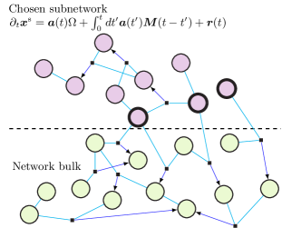
Our approach starts from kinetic equations for the concentrations of a set of molecular species in a large protein interaction network, allowing for small amounts of intrinsic noise caused by fluctuations in the copy number of each species as shown in Fig. 2a. We then use a projection operator formalism to obtain a set of dynamical equations for selected variables from the network, which define the chosen subnetwork. This approach retains information from the remainder of the larger network, i.e. the bulk, and allows us to obtain a reduced set of equations for the subnetwork (Fig. 2b). These projected equations contain extrinsic noise arising from the bulk dynamics as expected, but crucially the noise is accompanied by memory terms (Fig. 1). The memory terms are represented mathematically as integrals over the past history of the subnetwork, modulated by memory functions. These are the focus of our analysis. In Section 2 we explain the projection approach and how it can be applied to protein interaction networks. We also to illustrate the method with a simple example that already captures some general properties of memory functions (Fig. 2c). Next, in Section 3 we obtain closed-form expressions for memory functions in protein interaction network dynamics and discuss and illustrate some of their properties, e.g. the amplitudes and what they us about reactions between the subnetwork and the bulk. Finally in Section 4 we apply our approach to the EGFR protein signalling network for short-term signalling from Kholodenko et al. [2] and study the memory functions for a chosen subnetwork (Fig. 2d). We analyse the dominant contributions to the memory functions, and show that our projected equations with memory give a significantly more accurate description of the subnetwork dynamics than can be obtained without memory.

This paper makes two main contributions. The first is a demonstration of the conceptual and quantitative need to include memory terms in the description of generic subnetwork dynamics. The second is of a more technical nature, namely the derivation of closed-form memory functions for the full nonlinear dynamics of protein interaction networks. To reflect this contribution, and because the application of projection methods to derive memory effects in biological networks is novel, we describe the calculations in some detail. This is done in Sec. 3.1 for dynamics linearised around a fixed point and then for the full nonlinear dynamics in Sec. 3.2. Readers more interested in the conceptual aspects and applications of our work might wish to skip these sections. A graphical overview of the content of the paper is given in Fig. 2.

(a)

(b)

(c)

(d)

Figure 2: (a) Description of protein interaction networks: we use mass action kinetics ($x_{i}$, concentration of species $i$ = particle number per unit volume) with rates of binary complex formation and dissociation ($k^{+}_{ij,{l}},k^{-}_{{l},ij}$) and unary transformation ($\lambda_{lm}$). Reaction equations can be written in terms of the stoichiometry matrix ${\bf S}$ and reaction flux vector ${\bf f}$ (Sec. 2.1). Copy number fluctuations add intrinsic noise ${\bm{\eta}}$ with strength $\epsilon=1/V$, the inverse volume of the system (Sec. 2.2). (b) Factor graph representation: a square denotes an interaction, an arrow points to the resulting complex. The network is divided into the subnetwork of interest (purple nodes, upper) and the “bulk” (green nodes, lower). The time evolution of concentrations $\mathbf{x}$ within the subnetwork is described by projected equations (Sec. 2.3), where $\bm{a}(t)$ includes $\bm{x}^{\text{s}}$ and its products (Sec. 2.4). The rate matrix $\mathbf{\Omega}$ describes contributions that are local in time. Memory functions $\mathbf{M}(t)$ determine how strongly past values of $\mathbf{x}$ affect the present rates of change $\partial_{t}x_{i}(t)$ (Secs. 2.5, 3.1, 3.2); the random force $\mathbf{r}(t)$ represents extrinsic noise. Memory terms feature the history of species on the boundary of the subnetwork only (bold nodes, Sec. 3.3.1). (c) Exemplar subnetwork-bulk interactions for the calculation and properties of memory functions (Secs. 3.3.2). In a larger subnetwork, a memory function resulting from multiple reactions may be decomposed into “source” and “receiver” channels using these simple interaction structures (Sec. 3.3.3). (d) Application to a model of the EGFR signalling pathway (Secs. 4.1, 4.2; see Fig. 8 for full network). The bulk (green nodes) is chosen to be Shc and complexes containing Shc. The boundary species appearing in the memory terms are SOS, GS, Grb and RP (bold). Quantitative comparisons shows that accurate modelling of subnetwork time courses requires the inclusion of memory terms (Sec. 4.4).

2 Projection

2.1 Reaction equations

We consider a protein interaction network described using mass action kinetics. The molecular reactions can be either binary or unary. In a binary reaction two molecules react to form a molecule of a different species (complex formation); the reverse process is the dissociation of a complex into two molecules. In a unary reaction, one species transforms into another via a conformational change like phosphorylation. In our setup we do not restrict the nature of the molecules that come together in a binary reaction, and in particular we include the possibility that a complex formed in some initial binary reaction may react again with another molecule to form a higher order complex. As a convenient notational shorthand we nevertheless refer generically to the two molecules that join together in a binary reaction as “proteins”, and to the molecule that is formed as a complex.

The deterministic reaction equations for such a protein interaction network containing $N$ molecular species can be written in the form

$$\begin{split}\frac{\partial}{\partial t}x_{i}&=\sum_{j(\neq i),l}\left(k^{-}_{{l},ij}x_{l}-k^{+}_{ij,{l}}x_{i}x_{j}\right)+\frac{1}{2}\sum_{j\neq l}\left(k^{+}_{jl,{i}}x_{j}x_{l}-k^{-}_{{i},jl}x_{i}\right)\\ &\quad+\sum_{l}\left(2k^{-}_{{l},ii}x_{l}-k^{+}_{ii,{l}}x_{i}x_{i}\right)+\sum_{j}\left(\frac{1}{2}k^{+}_{jj,{i}}x_{j}x_{j}-k^{-}_{{i},jj}x_{i}\right)\\ &\quad+\sum_{j}\left(\lambda_{ji}x_{j}-\lambda_{ij}x_{i}\right)\end{split}$$ (1)

where $x_{i}$ is the concentration of species $i$. In our notation we follow to a large extent the paper by Coolen and Rabello [21], which presented an average-case analysis using generating functionals of the dynamics in large protein interaction networks. We denote by $k^{+}_{ij,{l}}$ the rate of formation of complex $l$ from proteins $i$ and $j$, and by $k^{-}_{{l},ij}$ the rate for the reverse process of dissociation of complex $l$ into proteins $i$ and $j$. To avoid ordering restrictions on the protein indices we set $k^{+}_{ij,{l}}=k^{+}_{ji,{l}}$ and $k^{-}_{{l},ij}=k^{-}_{{l},ji}$. The factor of 1/2 in the first line above is then needed to avoid double counting of reactions of two different molecular species. The second line relates to homodimer formation and dissociation, where two proteins of the same species $i$ react. The extra factor of 2 arises because dissociation of a homodimer $l$ creates two molecules of species $i$. The factor $1/2$ in the term describing formation of $i$ from two molecules of species $j$ represents the reduction in number of possible reaction pairs, compared to the case of formation of a heterodimer where the two reacting species are different. The unit prefactor of the $k^{+}_{ii,{l}}$ term arises as the combination of these two effects. Finally, the last line of (1) accounts for unary reactions, with $\lambda_{ij}$ the rate of species $i$ changing into species $j$.

The reaction equations (1) can be written in terms of a stoichiometry matrix and vector of reaction fluxes. Let the number of reactions with nonzero rates be $R$, where each forwards and backwards reaction is counted separately. Then the stoichiometry matrix $\bm{S}$ is made up of integers $S_{i\mu}$, with $i=1,2,\ldots,N$ and $\mu=1,2,\ldots,R$. Each $S_{i\mu}$ records by how much the molecule count of species $i$ changes in reaction $\mu$. Specifically, $S_{i\mu}$ is $-1$ if the molecular species $x_{i}$ is a reactant in reaction $\mu$ and $+1$ if it is a reaction product. For homodimer reactions one correspondingly has $S_{i\mu}=\pm 2$ when two molecules of species $i$ are used up or produced.

The vector of reaction fluxes $\bm{f}$ has entries $f_{\mu}$ that give the reaction rate of reaction $\mu$ multiplied by the concentrations of the proteins involved in that reaction. For example the flux related to the formation of a complex $x_{i}$ from proteins $j$ and $l$ is $k^{+}_{jl,{i}}x_{j}x_{l}$ and the reverse reaction flux is $k^{-}_{{i},jl}x_{i}$. For the conformational change of protein $i$ to protein $j$ the forward reaction has reaction flux $\lambda_{ij}x_{i}$ and the reverse reaction flux is $\lambda_{ji}x_{j}$.

With the stoichiometry matrix $\bm{S}$ and reaction flux vector $\bm{f}$ defined as above, the reaction equations (1) can be written in the compact form $\partial_{t}x_{i}=\sum_{\mu}S_{i\mu}f_{\mu}$. One benefit of this formulation is that it shows transparently how conservation laws arise, where the sum of a number of concentrations is constant in time. Quantitatively, the number of conservation laws is given by the dimension of the left nullspace of $\bm{S}$. If this nullspace is spanned by the (column) vectors $\bm{e}^{(a)}$, $a=1,2,\ldots$ then each such vector obeys $\bm{e}^{(a)^{{\rm T}}}\bm{S}=0$. Accordingly the quantity $\sum_{i}x_{i}e^{(a)}_{i}$ is conserved: $\partial_{t}\sum_{i}x_{i}e^{(a)}_{i}=\bm{e}^{(a)^{{\rm T}}}\bm{S}\bm{f}=0$.

2.2 Stochastic Dynamics

The deterministic reaction equations (1) apply in the case where the number of molecules of each species, $x_{i}V$ in a reaction compartment of volume $V$, is large enough so that stochastic fluctuations around the mean value can be neglected. In reality such copy number fluctuations are always present because the number of molecules of any species is discrete, and when it changes over time it does so due to elementary reactions that take place stochastically. The relative size of the fluctuations in any $x_{i}$ will be of order $1/\sqrt{x_{i}V}$, because any change in $x_{i}$ results from the cumulative effect of many reactions and the number of reactions occurring within any fixed time interval grows lineary with $V$.

We therefore next describe the stochastic extension of (1) to the case of small copy number fluctuations. The inverse volume of the system, $\epsilon=1/V$, will be used to characterize the strength of this intrinsic noise. We note that such a stochastic description is also important for our use of the projection operator formalism [22] to derive subnetwork dynamical equations, as this approach starts from the time evolution of a probability distribution over states of the network.

For small $\epsilon$, the appropriate stochastic version of (1) is a Fokker-Planck equation for the time evolution of the probability density $P(\bm{x},t)$. Truncating a Kramers-Moyal expansion [23] after the first order in $\epsilon$, this equation can be written in terms of the stoichiometry matrix, $\bm{S}$, and reaction flux vector, $\bm{f}$, as

$$\frac{\partial P(\bm{x},t)}{\partial t}=-\frac{\partial}{\partial\bm{x}}\left(\bm{Sf}P\right)+\frac{\epsilon}{2}\frac{\partial^{2}}{\partial\bm{x}^{2}}\left(\bm{BB}^{{\rm T}}P\right)=\mathcal{L}^{{\rm T}}P(\bm{x},t)$$ (2)

where

$$\bm{BB}^{{\rm T}}=\bm{S}\,\text{diag}\left(\bm{f}\right)\bm{S}^{{\rm T}}$$ (3)

and $\epsilon={1}/{V}$ is the inverse reaction volume as before. This formulation is useful for us as we can continue to describe each species concentration with a single variable $x_{i}$, rather than having to treat its mean time evolution and fluctuations separately as would be done in a van Kampen system size expansion [24, 25]. Moreover, a recent analysis [26] shows that (2) is more accurate than the van Kampen description, capturing the mean and variance of the $x_{i}$ to higher order in $\epsilon$.

We will sometimes find it useful to switch from the above Fokker-Planck description to the corresponding “chemical Langevin equation” [27], which reads

$$\frac{\partial}{\partial t}\bm{x}=\bm{Sf}\bm{x}+\bm{\eta}$$ (4)

The noise $\bm{\eta}$ is multiplicative as its statistics depend on $\bm{x}$; adopting the Ito interpretation [23], one has explicitly $\langle\bm{\eta}(t)\bm{\eta}^{{\rm T}}(t^{\prime})\rangle=\epsilon\bm{BB}^{{\rm T}}\delta(t-t^{\prime})$.

Returning to the Fokker-Planck equation (2), the time evolution it encodes can be thought of in terms of either an evolving $P(\bm{x},t)$ or evolving observables $a(\bm{x},t)$ of the system; see e.g.[22, 28]. The time variation of $P(\bm{x},t)$ is the solution of (2), which can be written formally as $P(\bm{x},t)=e^{\mathcal{L}^{{\rm T}}t}P(\bm{x},0)$. Here the operator exponential in $e^{\mathcal{L}^{{\rm T}}t}$ is defined as $e^{\mathcal{L}^{{\rm T}}t}=\sum_{n=0}^{\infty}(\mathcal{L}^{{\rm T}}t)^{n}/n!$, requiring in principle the application of successive powers of $\mathcal{L}^{{\rm T}}t$ to $P(\bm{x},0)$.

Now let $a(\bm{x})$ be an observable of the system, for example one of the protein concentrations $x_{i}$. Its time average evolves in time as

$$\begin{split}\langle a(t)\rangle&=\int d\bm{x}\ a(\bm{x})P(\bm{x},t)=\int d\bm{x}\ a(\bm{x})e^{\mathcal{L}^{{\rm T}}t}P(\bm{x},0)\end{split}$$ (5)

Here we have introduced $\mathcal{L}$ as the adjoint operator to $\mathcal{L}^{{\rm T}}$, defined by $\int d\bm{x}\,(\mathcal{L}a(\bm{x}))b(\bm{x})=\int d\bm{x}\,a(\bm{x})\mathcal{L}^{{\rm T}}b(\bm{x})$. We have also defined

$$a(\bm{x},t)=e^{\mathcal{L}t}a(\bm{x})$$ (6)

As the last equality of (5) shows, this is the average value of $a$ at time $t$ conditional on the system initially being in state $\bm{x}$. Its time evolution is given by (6), and reads in differential form

$$\partial_{t}a(\bm{x},t)=\mathcal{L}a(\bm{x},t)$$ (7)

with initial condition $a(\bm{x},0)=a(\bm{x})$.

Before we write down the adjoint Fokker-Planck operator, we make a change of variables. For reasons explained further in Section 2 below, it will be useful to have variables with a mean value of zero in steady state. We therefore define $\bm{x}=\bm{y}+\bm{\delta x}$ where $\bm{y}$ is the mean steady state value of $\bm{x}$, calculated as the fixed point of the mass-action equations (1), and $\bm{\delta x}$ is the deviation away from this. Where the meaning is clear from the context, we will then often use the shorthand “concentration” for the concentration deviations from steady state, $\delta x_{i}$. The time-evolving probability distribution is then $P(\bm{\delta x},t)$, and observables $a(\bm{\delta x})$ are likewise functions of $\bm{\delta x}$. In terms of these variables the adjoint Fokker-Planck operator $\mathcal{L}$ then writes

$$\begin{split}\mathcal{L}&=\sum_{i,j,l:i\neq j}\left[k^{-}_{{l},ij}\delta x_{l}-k^{+}_{ij,{l}}(y_{j}\delta x_{i}+y_{i}\delta x_{j}+\delta x_{i}\delta x_{j})\right]\frac{\partial}{\partial\delta x_{i}}\\ &\quad+\frac{1}{2}\sum_{i,j,l:j\neq l}\left[k^{+}_{jl,{i}}(y_{l}\delta x_{j}+y_{j}\delta x_{l}+\delta x_{j}\delta x_{l})-k^{-}_{{i},jl}\delta x_{i}\right]\frac{\partial}{\partial\delta x_{i}}\\ &\quad+\sum_{i,j}\biggl{\{}\left[2k^{-}_{{j},ii}\delta x_{j}-k^{+}_{ii,{j}}(2y_{i}\delta x_{i}+\delta x_{i}\delta x_{i})\right]\\ &\quad+\left.\frac{1}{2}\left[k^{+}_{jj,{i}}(2y_{j}\delta x_{j}+\delta x_{j}\delta x_{j})-k^{-}_{{i},jj}\delta x_{i}\right]\right\}\frac{\partial}{\partial\delta x_{i}}\\ &\quad+\sum_{i,j}\left(\lambda_{ji}\delta x_{j}-\lambda_{ij}\delta x_{i}\right)\frac{\partial}{\partial\delta x_{i}}+\frac{\epsilon}{2}\sum_{i,j}\left(\bm{BB}^{{\rm T}}\right)_{ij}\frac{\partial^{2}}{\partial\delta x_{i}\,\partial\delta x_{j}}\end{split}$$ (8)

All terms here except for the last describe deterministic evolution. To write the reaction flux prefactors from (1) we have replaced $x_{i}=y_{i}+\delta x_{i}$ and exploited the fact that when $\bm{x}=\bm{y}$, i.e. $\bm{\delta x}=0$, the deterministic drift terms must vanish. Note that $\mathcal{L}c=0$ for any constant $c$, so that from (7) the average of such an “observable” is constant in time as it should be. Looking at (5), this property is equivalent to conservation of probability in the original Fokker-Planck equation.

2.3 Projection method

We next summarise the salient features of the Zwanzig-Mori projection method we use to derive equations describing the time evolution of the concentrations in any chosen subnetwork of a larger protein interaction network [22, 29, 28]. The approach allows one generally to derive such equations for the conditional averages $a_{i}(\bm{\delta x},t)$ of any chosen set of observables $\{a_{\alpha}(\bm{\delta x})\}$. One first defines a projection operator $\mathcal{P}$ that projects any observable $b$ onto the space spanned by the chosen set of observables:

$$\left(\mathcal{P}b\right)(\bm{\delta x})=\sum_{\alpha,\beta}a_{\beta}(\bm{\delta x})\left(\bm{C}^{-1}\right)_{\beta\alpha}\left(a_{\alpha},b\right)$$ (9)

Here $\bm{C}$ is a correlation matrix with elements

$$C_{\alpha\beta}=\left(a_{\alpha},a_{\beta}\right)$$ (10)

defined in terms of an inner product $\left(a,b\right)$. The latter is just an average over the steady state distribution $P_{\text{ss}}(\bm{\delta x})$ of $\bm{\delta x}$:

$$\left(a,b\right)=\langle ab\rangle_{\text{ss}}=\int d\bm{\delta x}\ a(\bm{\delta x})b(\bm{\delta x})P_{\text{ss}}(\bm{\delta x}).$$ (11)

We see now explicitly that we need stochastic dynamics, i.e. nonzero $\epsilon$, to be able to deploy the projection formalism, even if we are interested in the limit of small $\epsilon$. If we were to set $\epsilon=0$ directly, the steady state distribution would become a Dirac delta function at the fixed point $\bm{\delta x}=0$, giving for the covariance matrix $C_{\alpha\beta}=a_{\alpha}(0)a_{\beta}(0)$. As the outer product of a vector – with elements $a_{\alpha}(0)$ – with itself this has rank one and so is not invertible except in the case of a single observable, making the projection operator (9) ill-undefined.

Once $\mathcal{P}$ is defined, the orthogonal projection operator $\mathcal{Q}$ follows as $\mathcal{Q}=1-\mathcal{P}$. Then $\mathcal{Q}b$ can be interpreted as the contribution to observable $b$ that is uncorrelated in steady state with any of the chosen observables $a_{i}$. In our case the latter will be a set of obervables from the system such as protein and complex concentrations from the subnetwork, as discussed in more detail below.

With the shorthand $a_{\alpha}(\bm{\delta x},t)=a_{\alpha}(t)$, the projected equations are written [22, 29, 28]

$$\frac{\partial}{\partial t}a_{\alpha}(t)=\sum_{\beta}a_{\beta}(t)\Omega_{\beta\alpha}+\int_{0}^{t}dt^{\prime}\sum_{\beta}a_{\beta}(t^{\prime})M_{\beta\alpha}(t-t^{\prime})+r_{\alpha}(t)$$ (12)

The first term on the r.h.s. is local in time. We will call the coefficients

$$\Omega_{\beta\alpha}=\sum_{\gamma}\left(\bm{C}^{-1}\right)_{\beta\gamma}\left(a_{\gamma},\mathcal{L}a_{\alpha}\right)$$ (13)

the elements of the rate matrix $\bm{\Omega}$; in other contexts, e.g. systems with inertial dynamics, it is often referred to as the frequency matrix. The second term represents the memory effects, as an integral over past values of the observables weighted by a function of the time lag, the memory function. The latter can be expressed as

$$M_{\beta\alpha}(\Delta t)=\sum_{\gamma}\left(\bm{C}^{-1}\right)_{\beta\gamma}\left(a_{\gamma},\mathcal{LQ}e^{\mathcal{QLQ}\Delta t}\mathcal{QL}a_{\alpha}\right)$$ (14)

where $\Delta t=t-t^{\prime}$. The memory function $M_{\beta\alpha}$ determines how strongly the past values of observable $a_{\beta}$ affect the present rate of change of $a_{\alpha}$; sometimes it will be useful to think of the $M_{\beta\alpha}(\Delta t)$ as the elements of a memory matrix $\bm{M}(\Delta t)$ whose size is, as for the rate matrix, the number of observables $a_{\alpha}$. The third term in (12), finally, is called the random force and is written

$$r_{\alpha}(t)=e^{\mathcal{QLQ}t}\mathcal{QL}a_{\alpha}.$$ (15)

The name comes from the fact that the value of $r_{\alpha}(t)$ at any time $t$ is uncorrelated with the initial values of the observables $a_{\beta}(0)\equiv a_{\beta}$; mathematically this property is expressed as $\left(a_{\alpha},r_{\beta}(t)\right)=0$. Note that this notion of randomness does not imply that the random force resembles white noise as in e.g. Langevin equations. This is natural given that it appears in the time evolution of the $a_{\alpha}(t)$, which are conditional averages over dynamical fluctuations. In fact we will see later in (37) that the random force encodes primarily the initial conditions of the bulk variables.

The projected equations (12) are exact as written, and have several remarkable features. Firstly, they emphasize that memory terms must arise generically once we go from a description of the full system, in terms of $\bm{\delta x}$, to one in terms of a reduced number of observables. Secondly, they provide an “almost” closed set of equations for the chosen observables, with all non-autonomous effects collected in the random force term. Specifically, while the time evolution of each $a_{\alpha}(\bm{\delta x},t)$ depends in principle on all details of the initial system state $\bm{\delta x}$, the projected equations (12) with the random force term omitted can be solved knowing only the initial values of the chosen observables, $a_{\alpha}(0)$.

To make use of the projected equations, we must be able to calculate the rate matrix and the memory functions, and say something about the statistics of the random force. Calculations of the rate matrix (13) and memory functions (14) are discussed in more detail in Section 3. Here we note only two useful identifies, which follow from the definitions of these quantities and that of the projection operator (9):

$$\begin{split}\sum_{\beta}a_{\beta}\Omega_{\beta\alpha}&=\mathcal{PL}a_{\alpha}\\ \sum_{\beta}a_{\beta}M_{\beta\alpha}(\Delta t)&=\mathcal{PLQ}e^{\mathcal{QLQ}\Delta t}\mathcal{QL}a_{\alpha}\\ \end{split}$$ (16)

To find $\Omega_{\beta\alpha}$ and $M_{\beta\alpha}(\Delta t)$ we can then first evaluate the r.h.s. of these identities, and identify the coefficients of the different $a_{\beta}$.

As regards the statistics of the random force, there is a simple scenario where all correlation functions $\langle r_{\gamma}(t^{\prime})r_{\alpha}(t)\rangle$ (for $t\geq t^{\prime}$) can be deduced from the memory functions. This is the case where the operator $\mathcal{L}$ is self-adjoint with regards to the product $(a,b)$, such that $(a,\mathcal{L}b)=(\mathcal{L}a,b)$ for any observables $a$ and $b$. Using that $\mathcal{Q}$ automatically has the same property one then finds [22, 29]

$$\sum_{j}C_{\gamma\beta}M_{\beta\alpha}(t-t^{\prime})=\left(\mathcal{QL}a_{\gamma},e^{\mathcal{QLQ}(t-t^{\prime})}\mathcal{QL}a_{\alpha}\right)=\left(e^{\mathcal{QLQ}t^{\prime}}\mathcal{QL}a_{\gamma},e^{\mathcal{QLQ}t}\mathcal{QL}a_{\alpha}\right)=\langle r_{\gamma}(t^{\prime})r_{\alpha}(t)\rangle$$ (17)

showing that random force correlators are indeed determined by the memory functions. The self-adjointness of $\mathcal{L}$ required here normally holds in physical systems: these obey detailed balance, meaning that in the steady state there are no unbalanced probability fluxes. Protein interaction networks do not in general have this property , so that random force statistics have to be calculated separately. We therefore leave this matter as a point of investigation for a separate publication, and note here only that the random force has the biological meaning of extrinsic noise acting on the subnetwork, arising from it being embedded in the bulk network.

What specific projected equations one obtains from the framework summarised above is of course largely dependent on the choice of observables $a_{\alpha}$. This is discussed in more detail in Sec. 2.4. Here we just note that one useful convention is to employ observables with vanishing steady state average, $\langle a_{\alpha}\rangle\equiv(a_{\alpha},1)=0$, which can always be achieved by subtracting any nonzero average from $a_{\alpha}$. This convention has two benefits: first, it guarantees that the matrix $\bm{C}$ defined in (10) really is a correlation matrix for fluctuations around the steady state. Second, the projection operator then obeys $\mathcal{P}c=0$, hence $\mathcal{Q}c=c$ and $\mathcal{QLQ}c=\mathcal{QL}c=0$. The operator $\mathcal{QLQ}$ thus inherits from $\mathcal{L}$ the property that its application to any constant gives zero. As argued above for $\mathcal{L}$, this is equivalent to saying that the adjoint operator $(\mathcal{QLQ})^{{\rm T}}$ conserves probability in the time evolution it generates. One can therefore think of the time-dependencies in the memory function and random force as resulting from a “projected evolution” of the system with this operator. In applications to physical systems, this is often used to argue that as a first approximation $\mathcal{QLQ}$ can be replaced by $\mathcal{L}$ [30, 31], though this is not a path we follow here as we want to retain a quantitatively accurate projected description.

In order to evaluate the rate matrix (13) and memory functions (14) we have to calculate the various observable products $(a,b)$ that occur, and from (11) these are defined in terms of the steady state distribution of $\bm{\delta x}$. In our case the latter is a vector of concentrations, shifted to zero mean. Our general strategy will be to consider suitably large reaction volumes so that the noise strength $\epsilon=1/V$ is small. More specifically we require that for typical concentrations of any species, the absolute number of molecules be large, say $Vy_{i}\gg 1$ for all $i$ if we take the steady state concentrations as typical. The steady state fluctuations $\bm{\delta x}$ will then be small, and we can find their distribution as the steady state to an approximate Fokker-Planck operator, obtained from $\mathcal{L}^{{\rm T}}$ by linearizing around $\bm{\delta x}=0$. We emphasise that this simplification is used only for the steady state, and does not restrict the deviations from the steady state $\bm{\delta x}$ that can be considered in the projected equations, e.g. while the system evolves from some non-steady initial state.

In the linearised version of $\mathcal{L}$, the diffusion matrix $\bm{BB}^{{\rm T}}$ is evaluated at $\bm{\delta x}=0$, i.e. at the steady state concentrations. The deterministic drift is linearised in $\bm{\delta x}$ so that it can be written in terms of a drift matrix $\bm{A}$ and a vector $\bm{\delta x}$ as $\bm{Sf}=\bm{A\delta x}$. The steady state $P_{\text{ss}}(\bm{\delta x})$ of such a Fokker-Planck operator is a Gaussian distribution for the $\bm{\delta x}$ with zero mean and a covariance matrix $\bm{\Sigma}$ that is a solution of the Lyapunov equation [34]

$$\bm{A\Sigma}+\bm{\Sigma A}^{\rm T}+\epsilon\bm{BB}^{{\rm T}}=0$$ (18)

Once $\bm{\Sigma}$ is known, the inner products (11) in the projection can then be evaluated as Gaussian averages.

One proviso with this approach to finding $\bm{\Sigma}$, and hence $P_{\rm ss}(\bm{\delta x})$, is that the solution to the Lyapunov equation is not unique. This is because of the conservation laws: each fixed value of the conserved quantities leads to a different steady state distribution, and the generic solution for $\bm{\Sigma}$ represents a superposition of these distributions. In simple networks that we have analysed – and more generally in any network with the detailed balance property discussed above – one particularly simple solution of this type is the one where each molecular species has independent Poisson fluctuations at steady state. For small $\epsilon$ this product of Poisson distributions becomes a Gaussian with a diagonal covariance matrix $\bm{\Sigma}$. Because under Poisson statistics the variance of the number of molecules for each species, $Vx_{i}$, equals its mean $Vy_{i}$, one has $\langle(V\delta x_{i})^{2}\rangle=Vy_{i}$ and hence $\Sigma_{ii}=\langle(\delta x_{i})^{2}\rangle=y_{i}/V=\epsilon y_{i}$. For brevity we will call such a covariance matrix “Poissonian”.

We will see below that having a steady state distribution with Poissonian covariance matrix has a number of benefits. The main one is that the rate matrix terms in the projected equations will reproduce precisely those terms from the original evolution equations for the full network that describe reactions within the chosen subnetwork. The memory terms can then be interpreted directly as arising from the presence of the bulk. In view of this, we will use the Poissonian choice of covariance matrix throughout. This means that, depending on the network under study, one $P_{\text{ss}}(\bm{\delta x})$ will only be an approximation of the true steady state distribution. However, this is not a serious obstacle: if one looks at the derivation [22] of the projected equations (12), one sees that in principle any distribution can be used to define the projection operator. (The exception is the detailed balance property discussed around (17), but we do not rely on this in our analysis.) The price we pay is that the random force is then “random”, i.e. uncorrelated with the initial values of our chosen observables, under the Poisson distribution we have chosen, while under the true steady state distribution it will generally have nonzero correlations. This is a proviso that has to be born in mind, but it is easily outweighed by the fact that the projected equations will be simpler to interpret.

In summary, while the Poissonian covariance matrix assumption does represent a valid steady state in simple networks, more generally it should be viewed as an auxiliary construct that produces the simplest form of the projected equations for the subnetwork dynamics.

2.4 Choice of subnetwork observables

Figure 3: Sketch of a simple model protein interaction network. Protein 1 reacts with protein 2 to form complex 3, and in reverse 3 can dissociate into 1 and 2. There is an analogous reaction where 1 reacts with 4 to form 5, and the reverse dissociation. We choose the subnetwork to be species 1, 2 and 3 and the bulk to be 4 and 5, as indicated by the dashed line.

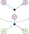
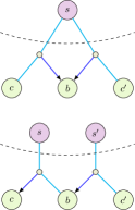
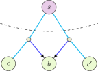
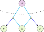
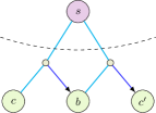
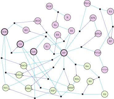
To calculate the projected equations we need to choose the set of observables $\{a_{i}(\bm{\delta x})\}$ that we will project on. We assume that a set of molecular species has been chosen as the subnetwork of interest, e.g. because of relevance to some biological function or experimental accessibility. As before we will call the rest of the species in the network the bulk. However, this division still leaves an element of choice in which subnetwork observables to use in the projection. To illustrate the issues, we consider a small example, represented graphically in Figure 3, with two complex formation and dissociation reactions as indicated below:

$$\begin{split}1+2&\xrightleftharpoons[k^{-}_{{3},12}]{k^{+}_{12,{3}}}3\\ 1+4&\xrightleftharpoons[k^{-}_{{5},14}]{k^{+}_{14,{5}}}5\end{split}$$ (19)

The chemical Langevin equations for this network are

$$\begin{split}\frac{\partial}{\partial t}\delta x_{1}&=k^{-}_{{3},12}\delta x_{3}-k^{+}_{12,{3}}\left(y_{2}\delta x_{1}+y_{1}\delta x_{2}+\delta x_{1}\delta x_{2}\right)\\ &\quad+k^{-}_{{5},14}\delta x_{5}-k^{+}_{14,{5}}\left(y_{4}\delta x_{1}+y_{1}\delta x_{4}+\delta x_{1}\delta x_{4}\right)+\eta_{1}\\ \frac{\partial}{\partial t}\delta x_{2}&=k^{-}_{{3},12}\delta x_{3}-k^{+}_{12,{3}}\left(y_{2}\delta x_{1}+y_{1}\delta x_{2}+\delta x_{1}\delta x_{2}\right)+\eta_{2}\\ \frac{\partial}{\partial t}\delta x_{3}&=k^{+}_{12,{3}}\left(y_{2}\delta x_{1}+y_{1}\delta x_{2}+\delta x_{1}\delta x_{2}\right)-k^{-}_{{3},12}\delta x_{3}+\eta_{3}\\ \end{split}$$ (20a)

$$\begin{split}\frac{\partial}{\partial t}\delta x_{4}&=k^{-}_{{5},14}\delta x_{5}-k^{+}_{14,{5}}\left(y_{4}\delta x_{1}+y_{1}\delta x_{4}+\delta x_{1}\delta x_{4}\right)+\eta_{4}\\ \frac{\partial}{\partial t}\delta x_{5}&=k^{+}_{14,{5}}\left(y_{4}\delta x_{1}+y_{1}\delta x_{4}+\delta x_{1}\delta x_{4}\right)-k^{-}_{{5},14}\delta x_{5}+\eta_{5}\end{split}$$ (20b)

Here the terms $\eta_{i}$ are the contributions from the (intrinsic) noise. As in the general form of the adjoint Fokker-Planck operator (8), we have written concentration products $x_{i}x_{j}$ from the original mass action form (1) in terms of $\delta x_{i}$ and $\delta x_{j}$ and removed constant terms that cancel in steady state, giving $y_{j}\delta x_{i}+y_{i}\delta x_{j}+\delta x_{i}\delta x_{j}$.

We assume that the subnetwork of interest in this example consists of species 1, 2 and 3, and want to select observables for the projection method accordingly. The goal is to keep the number of variables small, for computational and conceptual expediency, while retaining an explicit description of the subnetwork reaction (20a) in its original form

As a first choice one could consider projecting onto only the protein concentrations in the subnetwork, $(\delta x_{1},\delta x_{2})$. Explicitly, this means we use only two observables, $a_{1}(\bm{\delta x})=\delta x_{1}$ and $a_{2}(\bm{\delta x})=\delta x_{2}$ where $\bm{\delta x}=(\delta x_{1},\ldots,\delta x_{5})^{\rm T}$. When we write down the projected equations (12), we should in principle write $a_{1}(t)$ and $a_{2}(t)$ and bear in mind that these are the conditional averages – over the stochastic noise from copy number fluctuations – of $\delta x_{1}$ and $\delta x_{2}$. However, as we are interested throughout in the limit of small $\epsilon$, where the effect of averaging over the noise becomes negligible, we write directly $\delta x_{1}$ and $\delta x_{2}$.

Deferring for now a discussion of how rate matrix and memory functions are calculated in practice (see Secs. 3.1 and 3.2), we state directly the projected equation for $\delta x_{1}$ that results from the above choice of subnetwork observables:

$$\begin{split}\frac{\partial}{\partial t}\delta x_{1}&=-k^{+}_{12,{3}}\left(y_{2}\delta x_{1}+y_{1}\delta x_{2}\right)-k^{+}_{14,{5}}y_{4}\delta x_{1}\\ &\quad+\int_{0}^{t}dt^{\prime}\left[k^{+}_{14,{5}}y_{4}(k^{-}_{{5},14}+k^{+}_{14,{5}}y_{1})e^{-(k^{-}_{{5},14}+k^{+}_{14,{5}}y_{1})(t-t^{\prime})}+k^{-}_{{3},12}k^{+}_{12,{3}}y_{2}e^{-k^{-}_{{3},12}(t-t^{\prime})}\right]\delta x_{1}(t^{\prime})\\ &\quad+\int_{0}^{t}dt^{\prime}\left[k^{-}_{{3},12}k^{+}_{12,{3}}y_{1}e^{-k^{-}_{{3},12}(t-t^{\prime})}\right]\delta x_{2}(t^{\prime})+r_{1}(t)\\ \end{split}$$ (21)

The terms from the rate matrix, which are the local-in-time contributions in the first line, are linear in $\delta x_{1}$ and $\delta x_{2}$ as expected from (12). They therefore do not capture all terms from the complex formation and dissociation reactions within the subnetwork, as written in the first line of (20a)

To include nonlinear terms, one could consider adding a third observable, $a_{3}=\delta x_{1}\delta x_{2}-\langle\delta x_{1}\delta x_{2}\rangle$, giving a projection onto protein concentrations and products of protein concentrations. We have written the subtraction of $\langle\delta x_{1}\delta x_{2}\rangle$ here for clarity to emphasize that also nonlinear observables must have zero mean, though for our chosen Poissonian steady state this average vanishes. The projected equation for $\delta x_{1}$ that results is similar to (21), but now explicitly includes the $\delta x_{1}\delta x_{2}$ term from the first line of (20a). However, the complex dissociation term $k^{-}_{{3},12}\delta x_{3}$ still does not feature because the complex, species 3, remains “eliminated” from the subnetwork description. Its contribution is retained indirectly through the memory function, but not in a very transparent way.

The best option is therefore to project onto the protein concentrations, products of protein concentrations and complex concentrations from the subnetwork. With the vector of observables now $(a_{1},\ldots,a_{4})=\left(\delta x_{1},\delta x_{2},\delta x_{3},\delta x_{1}\delta x_{2}-\langle\delta x_{1}\delta x_{2}\rangle\right)$, the projected equation for $\delta x_{1}$ becomes

$$\begin{split}\frac{\partial}{\partial t}\delta x_{1}&=k^{-}_{{3},12}\delta x_{3}-k^{+}_{12,{3}}\left(y_{2}\delta x_{1}+y_{1}\delta x_{2}+\delta x_{1}\delta x_{2}\right)-k^{+}_{14,{5}}y_{4}\delta x_{1}\\ &\quad+\int_{0}^{t}dt^{\prime}\left[M_{1,1}(t-t^{\prime})\delta x_{1}(t^{\prime})+M_{12,1}(t-t^{\prime})\delta x_{1}(t^{\prime})\delta x_{2}(t^{\prime})\right]+r_{1}(t)\end{split}$$ (22)

All contributions relating to the subnetwork reaction $1+2\xrightleftharpoons{}3$ now appear directly via the local-in-time rate matrix terms: compare the first line of (22) to (20a). The bulk, which here comprises just species 4 and 5, contributes an additional local-in-time term because of the reaction of $4$ with $1$. The other bulk effects are captured in the memory terms: as expected from our general discussion, feedback effects from the subnetwork into the bulk and back at a later time lead to the evolution of $\delta x_{1}$ being coupled linearly to its own history, via a “self memory” term; there is also memory term that is nonlinear in concentration fluctuations. The linear self-memory function can be written explicitly as $M_{1,1}(t-t^{\prime})=k^{+}_{14,{5}}y_{4}(k^{-}_{{5},14}+k^{+}_{14,{5}}y_{1})e^{-(k^{-}_{{5},14}+k^{+}_{14,{5}}y_{1})(t-t^{\prime})}$; we omit the full expression for $M_{12,1}(t-t^{\prime})$ for the sake of brevity. As expected, the reaction rates $k^{+}_{14,{5}}$ and $k^{-}_{{5},14}$ relating to the bulk protein and complex that are being projected out from the description appear in the memory functions.

The upshot of the discussion so far is that we should project onto the concentrations of all molecular species from the subnetwork – both proteins and complexes – and all products of these concentrations. This gives projected equations where (a) all reactions taking place within the subnetwork are represented in their original form, as if the subnetwork was isolated, and (b) memory terms arise only from the presence of the bulk. One final choice left open here is which concentration products to include, only those occurring in the subnetwork reactions like $\delta x_{1}\delta x_{2}$ above, or all possible concentration products (e.g. $\delta x_{1}\delta x_{2}$, $\delta x_{1}^{2}$, $\delta x_{2}^{2}$, with nonzero averages subtracted as necessary). We will see below that the latter choice has advantages in a general treatment, in that it leads to smaller random force contributions.

2.5 Memory functions: initial orientation

We conclude this section by using the simple example above to provide some initial insights into the properties and intuitive meaning of memory functions.

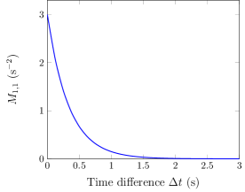
We focus initially on the self-memory function $M_{1,1}(t-t^{\prime})$. Figure 4 shows a sketch of this function, for a simple choice of reaction rates in appropriate dimensionless units. The self-memory function is positive, and decays exponentially with the time difference to the presence. The sign implies that having a higher concentration of species $1$ at some previous time $t^{\prime}$ ($\delta x_{1}(t^{\prime})>0$) will lead to more $1$ being created at time $t$. To see why this is so, note that if more 1 is present at $t^{\prime}$, then more of species $5$ will be created from the reaction with 4; this will then dissociate back into $1$ at a later time, increasing the concentration of $1$. This effect weakens as the concentration of 5 reverts to its steady state with time, explaining the decay of the memory function with the time difference $t-t^{\prime}$.

Figure 4: The coefficient of the self memory function for $\delta x_{1}$ with rate constants $k^{+}_{12,{3}}=k^{+}_{14,{5}}=1$, $k^{-}_{{3},12}=k^{-}_{{5},14}=2$, and steady state values $y_{1}=y_{2}=y_{3}=1$.

Looking at the self-memory function more quantitatively, one recognises that it reflects conservation laws of the proteins and complexes in the bulk, as it should. For the above example there is one such conservation law: the total concentration of species 4 and 5 is conserved, implying that deviations away from steady state are equal and opposite: $\delta x_{4}=-\delta x_{5}$. Therefore the equation (20b) for the complex $\delta x_{5}$ can be rewritten as

$$\frac{\partial}{\partial t}\delta x_{5}=k^{+}_{14,{5}}\left(y_{4}\delta x_{1}-\delta x_{1}\delta x_{5}\right)-\left(k^{+}_{14,{5}}y_{1}+k^{-}_{{5},14}\right)\delta x_{5}$$ (23)

If we now drop the $\delta x_{1}\delta x_{5}$ term, which would contribute to the random force and to nonlinear memory terms and then integrate this equation we obtain $\delta x_{5}(t)=\int_{0}^{t}dt^{\prime}k^{+}_{14,{5}}y_{4}e^{-(k^{-}_{{5},14}+k^{+}_{14,{5}}y_{1})(t-t^{\prime})}\delta x_{1}(t^{\prime})$ (up to an initial condition-dependent term which would give another contribution to the random force). Inserting into the equation for $\delta x_{1}$ in (20a) and using $\delta x_{4}=-\delta x_{5}$ then gives the linear memory term in (22), showing that this accounts for the bulk conservation law as it should.

If we next look at the general structure of the memory terms in the projected equation for (22), we notice that in the linear memory terms only the history of $\delta x_{1}$ features, not that of $\delta x_{2}$. The same is true in the projected equation of motion for $\delta x_{2}$, which we have not given explicitly. As explained in more detail in Section 3.3, this is a general property of linear memory terms: the only variables that appear in these are the concentrations of “boundary species”. Here a boundary species is one that has a direct reaction with a bulk species. In our example above, 1 is the only boundary species, while 2 and 3 are in the interior of the subnetwork. The intuitive reason why their histories do not appear in linear memory terms is that their effects on the bulk can only be “transmitted” indirectly via the time course of the concentration of species 1, rather than directly.

Figure 5: Concentration time courses for example (19), comparing the solution of the full reaction equations (20) (solid lines) and the solution of the subnetwork projected equations (22) (symbols). Note the excellent agreement even though random force terms were omitted from the projected equations. The $y$-axis shows fractional concentration deviations from the steady state, $\delta x_{i}/y_{i}$, so that a value of $-1$ corresponds to concentration $x_{i}=0$. Rate constants $k^{+}_{12,{3}}=k^{+}_{14,{5}}=1$ and $k^{-}_{{3},12}=k^{-}_{{5},14}=2$; initial conditions $\delta x_{1}(0)/y_{1}=\delta x_{2}(0)/y_{2}=1/2$, $\delta x_{3}(0)/y_{3}=-1$, $\delta x_{4}(0)=\delta x_{5}(0)=0$.

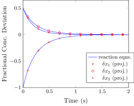
Finally we demonstrate the quantitative accuracy of the projected equations, i.e. (22) and the analogous equations for $\delta x_{2}$ and $\delta x_{3}$. We know that the equations are exact in the small noise limit $\epsilon\to 0$ that we have already taken, but the random force terms cannot be expressed in closed form, as discussed in more detail below. Our interest is therefore in assessing how accurate the projected subnetwork description is when the random force terms are omitted but memory terms are retained. Fig. 5 compares the solution of the resulting approximate projected equations with the solution of the full set of reaction equations (20). The two sets of time courses are visually indistinguishable, confirming that the projected subnetwork equations give a highly accurate description of the dynamics. The initial conditions were chosen so that concentrations of bulk species were at their steady state values. This is the regime where we expect the omitted random force terms to be smallest, as discussed in Sec. 4.4 below. We will also compare to alternative reduced descriptions of subnetwork dynamics.

3 Memory functions: explicit expressions and general properties

In this section we give explicit expressions for memory functions

describing the dynamics of protein interaction subnetworks. We study their general properties, in particular with a view to how they encode subnetwork-bulk interactions. In Sec. 3.1 we study first a simplified scenario, where the dynamical equations of the original large network are linearised around the steady state. Applying the projection method to obtain a description of the subnetwork dynamics, the memory functions can be found explicitly; we validate the approach by comparing with the simpler approach of integrating out the bulk degrees of freedom directly. In Sec. 3.2 we then demonstrate that, more surprisingly, we can obtain the memory functions explicitly even for the full nonlinear dynamics. Here as throughout we focus on the small noise, large reaction volume limit $\epsilon\to 0$. Finally, in Sec. 3.3 we discuss some generic properties of memory functions.

3.1 Linearised dynamics

To get some insight into the general form of the projected equations we first consider a simplified problem, starting from a linearised description for the full network. The linearised reaction equations including copy number noise are

$$\partial_{t}\bm{\delta x}=\bm{A\,\delta x}+\bm{\eta}$$ (24)

where $\bm{A}$ is as defined just before (18) and the covariance matrix $\epsilon\bm{B}\bm{B}^{\rm T}$ of the noise $\eta$, which normally is $\bm{\delta x}$-dependent, is evaluated at steady state ($\bm{\delta x}=0$). The corresponding adjoint Fokker-Planck operator is

$$\mathcal{L}=\sum_{ij}\delta x_{j}A_{ji}\frac{\partial}{\partial\delta x_{i}}+\frac{\epsilon}{2}\sum_{ij}(\bm{B}\bm{B}^{\rm T})_{ij}\frac{\partial^{2}}{\partial\delta x_{i}\partial\delta x_{j}}$$ (25)

In Section 2.4 we showed that in general, the most appropriate choice of subnetwork observables $\{a_{i}\}$ consists of the subnetwork concentrations and all their products. Now that we are considering linearised dynamics, we will only want to project onto the concentrations themselves, omitting the products. The linearised projected equations can then be written in the general form

$$\frac{\partial}{\partial t}\delta x_{i}(t)=\sum_{j=1}^{N^{\text{s}}}\delta x_{j}(t)\Omega_{ji}+\int_{0}^{t}dt^{\prime}\sum_{j=1}^{N^{\text{s}}}\delta x_{j}(t^{\prime})M_{ji}(t-t^{\prime})+r_{i}(t)$$ (26)

and our aim will be to find explicit expressions for the rate matrix entries $\Omega_{ji}$ and the memory functions $M_{ji}(t-t^{\prime})$. Note that, as it should be for a description of the subnetwork dynamics, the sums over $j$ above runs only over subnetwork concentrations. We assume here that these concentrations make up the first entries of the vector $\bm{\delta x}$, i.e. $x_{j}$ with $j=1\ldots N^{\text{s}}$ where $N^{\text{s}}$ is the number of subnetwork species. We will denote the subnetwork part of $\bm{\delta x}$ by $\bm{\delta x}^{\text{s}}$, and the remaining bulk part by $\bm{\delta x}^{\text{b}}$, so that $\bm{\delta x}^{{\rm T}}=(\bm{\delta x}^{\text{s}}{}^{\rm T},\bm{\delta x}^{\text{b}}{}^{\rm T})$.

To find the rate matrix and memory functions from the general expressions (13) and (14), or equivalently (16), we need to be able to find the action of the operators $\mathcal{L}$, $\mathcal{P}$ and $\mathcal{Q}$ on the observables $a_{i}=\delta x_{i}$ ($i=1,\ldots,N^{\text{s}}$) and evaluate products of the form $(a,b)$. Starting with the latter, we choose for the (approximate) steady-state distribution a Gaussian over $\bm{\delta x}$ with mean zero and Poissonian covariance matrix $\bm{\Sigma}$. The elements of this matrix then give the products $(\delta x_{i},\delta x_{j})=\Sigma_{ij}$. More specifically, if we partition the covariance matrix depending on whether the relevant molecular species are in the subnetwork or bulk, as done for the vector $\bm{\delta x}$, it can be written in the form

$$\bm{\Sigma}=\begin{pmatrix}\bm{\Sigma}^{{\rm{s},\rm{s}}}&\bm{0}\\ \bm{0}&\bm{\Sigma}^{{\rm{b},\rm{b}}}\end{pmatrix}$$ (27)

The Poissonian form for $\bm{\Sigma}$ forces zeros on the off-diagonal blocks as we have written. It also implies that $\bm{\Sigma}^{{\rm{s},\rm{s}}}$ are $\bm{\Sigma}^{\rm{b},\rm{b}}$ are diagonal, although we will not need this property in the following.

We can now write down the action of the projection operator (9) on a generic observable. For linear observables $\delta x_{i}$, which will be sufficient for our purposes, we obtain

$$\mathcal{P}\delta x_{i}=\sum_{j,k\leq N^{\text{s}}}\left(\delta x_{i},\delta x_{j}\right)\left(\bm{\Sigma}^{{\rm{s},\rm{s}}}\right)^{-1}{}_{jk}\delta x_{k}$$ (28)

Here we have used that the observable correlation matrix $\bm{C}$, i.e. covariance of the subnetwork concentrations, is just the top left block $\bm{\Sigma}^{\rm{s},\rm{s}}$ of $\bm{\Sigma}$. For $i=1,\ldots,N^{\text{s}}$ the first product is simply $\Sigma^{{\rm{s},\rm{s}}}_{ij}$ so that $\mathcal{P}\delta x_{i}=\delta x_{i}$. Conversely for $i=N^{\text{s}}+1,\ldots,N$ the product vanishes because of the block structure of $\bm{\Sigma}$, and $\mathcal{L}\delta x_{i}=0$. If we collect these results, and the corresponding ones for the orthogonal projector $\mathcal{Q}$, in the form

$$\begin{split}\mathcal{P}\delta x_{i}&=\sum_{j=1}^{N}\delta x_{j}P_{ji}\\ \mathcal{Q}\delta x_{i}&=\sum_{j=1}^{N}\delta x_{j}Q_{ji}\end{split}$$ (29)

then the coefficients $P_{ji}$ and $Q_{ji}$ can be arranged into matrices with the simple block form

$$\bm{P}=\begin{pmatrix}\mathbb{1}&\bm{0}\\ \bm{0}&\bm{0}\end{pmatrix},\quad\bm{Q}=\begin{pmatrix}\bm{0}&\bm{0}\\ \bm{0}&\mathbb{1}\end{pmatrix}$$ (30)

These results are intuitively obvious: when we project onto the subnetwork, the only observables that survive are those from the subnetwork. Similarly when applying the orthogonal projection operator $\mathcal{Q}$, only bulk observables remain.

Finally we can also write the adjoint Fokker-Planck operator in a similar matrix form. Looking at (25), $\mathcal{L}\delta x_{j}=\sum_{i}A_{ji}\delta x_{i}$, so if we define

$$\begin{split}\mathcal{L}\delta x_{i}&=\sum_{j=1}^{N}\delta x_{j}L_{ji}\end{split}$$ (31)

then $\bm{L}=\bm{A}^{\rm T}$ is the transpose of the dynamical matrix. This makes sense as the equation of motion (7) for the conditionally averaged concentrations,

$$\frac{\partial}{\partial t}\delta x_{i}=\mathcal{L}\delta x_{i}=\sum_{j}\delta x_{j}L_{ji}$$ (32)

has to agree with the noise-averaged rate equation (24), $\partial_{t}\delta x_{i}=\sum_{j}A_{ij}\delta x_{j}=\sum_{j}\delta x_{j}(\bm{A}^{{\rm T}})_{ji}$. We can partition the matrix $\bm{L}$ representing the adjoint Fokker-Planck operator $\mathcal{L}$ into subnetwork and bulk contributions again, according to

$$\bm{L}=\begin{pmatrix}\bm{L}^{{\rm{s},\rm{s}}}&\bm{L}^{{\rm{s},\rm{b}}}\\ \bm{L}^{{\rm{b},\rm{s}}}&\bm{L}^{{\rm{b},\rm{b}}}\end{pmatrix}$$ (33)

From the definition (31) one then sees that ${L}^{{\rm{b},\rm{s}}}$, for example, contains the coefficients of bulk concentrations in the equations of motion for subnetwork concentrations.

Note that the matrix representations (29) and (31) have been defined so that the vector $\bm{\delta x}$ sits on the left, e.g. $\mathcal{P}\bm{\delta x}^{\rm T}=\bm{\delta x}^{\rm T}\bm{P}$. This has the advantage of maintaining the ordering of the matrices when operators are composed, for example $\mathcal{PL}\delta x_{i}=\mathcal{P}\sum_{j}\delta x_{j}L_{ji}=\sum_{jk}\delta x_{k}P_{kj}L_{ji}$, or in vector form $\mathcal{PL}\bm{\delta x}^{\rm T}=\bm{\delta x}^{\rm T}\bm{PL}$.

This identity can now be employed directly to get the rate matrix terms in the projected equations (12). We use (16), i.e. $\sum{j=1}^{N^{\text{s}}}\delta x_{j}\Omega_{ji}=\mathcal{PL}\delta x_{i}$. This has to hold for all $i=1,\ldots,N^{\text{s}}$, so one reads off that $\bm{\Omega}$ is the top left block of $\bm{PL}$, which because of the simple form of (30) is simply the top left block of $\bm{L}$ in (33), i.e.

$$\bm{\Omega}=\bm{L}^{\rm{{s}},\rm{{s}}}$$ (34)

Similarly, the memory function obeys the identity (16):

$$\sum_{j=1}^{N^{\text{s}}}\delta x_{j}M_{ji}(t)=\mathcal{PLQ}e^{\mathcal{QLQ}t}\mathcal{QL}\delta x_{i}$$ (35)

Exploiting the correspondence between operators and matrices again, the r.h.s. is the $i$-th entry of the vector $\bm{\delta x}^{\rm T}\bm{PLQ}e^{\bm{QLQ}t}\bm{QL}$. Comparing with the l.h.s. shows that the matrix of memory functions $\bm{M}(t)$ is the top left block of $\bm{PLQ}e^{\bm{QLQ}t}\bm{QL}$, where $e^{\bm{QLQ}t}$ is a matrix exponential. Inserting the block decomposition (33) of $\bm{L}$ and exploiting again (30) shows that this can be written explicitly as

$$\bm{M}(t)=\bm{L}^{\rm{{s}},\rm{{b}}}e^{\bm{L}^{\rm{{b}},\rm{{b}}}t}\bm{L}^{\rm{{b}},\rm{{s}}}$$ (36)

With this and (34) we have obtained the desired explicit expressions for the rate and memory matrices of the projected equations (26). We note as an aside that, for the linearised scenario we are considering here, an expression for the random force can also be found. The definition (15) becomes $r_{i}(t)=e^{\mathcal{QLQ}t}\mathcal{QL}\delta x_{i}$, which is the $i$-th entry of the vector $\bm{\delta x}^{{\rm T}}e^{\bm{QLQ}t}\bm{QL}$. If we gather the required entries for $i=1,\ldots,N^{\text{s}}$ into a vector $\bm{r}(t)$, this can be simplified to

$$\bm{r}^{\rm T}(t)=\bm{\delta x}^{\text{b}}{}^{\rm T}e^{\bm{L}^{\rm{{b}},\rm{{b}}}}\bm{L}^{\rm{{b}},\rm{{s}}}.$$ (37)

We have gone through the application of the projection approach to the linearised dynamics to illustrate the steps involved in calculating the rate matrix and memory functions. For this relatively simple setup one can obtain the projected equations also more directly, by integrating out the bulk degrees of freedom. One starts from the equations of motion for the (conditionally averaged) concentrations, which read $\partial_{t}\bm{\delta x}^{\rm T}=\bm{\delta x}^{\rm T}\bm{L}$ or after decomposing into subnetwork and bulk terms

$$\partial_{t}\bm{\delta x}^{\text{s}}{}^{\rm T} =\bm{\delta x}^{\text{s}}{}^{\rm T}\bm{L}^{\rm{{s}},\rm{{s}}}+\bm{\delta x}^{\text{b}}{}^{\rm T}\bm{L}^{\rm{{b}},\rm{{s}}}$$ (38a)

$$\partial_{t}\bm{\delta x}^{\text{b}}{}^{\rm T} =\bm{\delta x}^{\text{s}}{}^{\rm T}\bm{L}^{\rm{{s}},\rm{{b}}}+\bm{\delta x}^{\text{b}}{}^{\rm T}\bm{L}^{\rm{{b}},\rm{{b}}}$$ (38b)

The solution for the bulk concentrations reads

$$\bm{\delta x}^{\text{b}}{}^{\rm T}(t)=\bm{\delta x}^{\text{b}}{}^{\rm T}(0)e^{\bm{L}^{\rm{{b}},\rm{{b}}}t}+\int_{0}^{t}dt^{\prime}\,\bm{\delta x}^{\text{s}}{}^{\rm T}(t^{\prime})\bm{L}^{\rm{{s}},\rm{{b}}}e^{\bm{L}^{\rm{{b}},\rm{{b}}}(t-t^{\prime})}$$ (39)

and substituting into the first line of (38a) gives for the subnetwork concentrations

$$\partial_{t}\bm{\delta x}^{\text{s}}{}^{\rm T}(t)=\bm{\delta x}^{\text{s}}{}^{\rm T}\bm{L}^{\rm{{s}},\rm{{s}}}+\int_{0}^{t}dt^{\prime}\,\bm{\delta x}^{\text{s}}{}^{\rm T}(t^{\prime})\bm{L}^{\rm{{s}},\rm{{b}}}e^{\bm{L}^{\rm{{b}},\rm{{b}}}(t-t^{\prime})}\bm{L}^{\rm{{b}},\rm{{s}}}+\bm{\delta x}^{\text{b}}{}^{\rm T}(0)e^{\bm{L}^{\rm{{b}},\rm{{b}}}t}\bm{L}^{\rm{{b}},\rm{{s}}}$$ (40)

which is exactly (26) with the rate matrix (34), memory matrix (36) and random force (37). This derivation shows explicitly how memory arises from bulk degrees of freedom being influenced by past behaviour of the subnetwork, and then feeding this influence back to the subnetwork at a later time. One also sees either from this or from (37) that the random force terms account for the effects of potentially unknown bulk initial conditions $\bm{\delta x}^{\text{b}}(0)$. When $\bm{\delta x}^{\text{b}}(0)=0$, i.e. when the bulk is initially in steady state, then the random force vanishes. The solution of the projected equations for the subnetwork with the random force omitted will then match exactly the solution of the original linearised reaction equations (32). This motivates the good agreement we observed between the two sets of solution in the simple example of Sec. 2.4, cf. Fig. 3, although there we were dealing with the full nonlinear reaction equations. This is the topic we consider next.

3.2 Nonlinear dynamics

The projection approach as examplified for linearised dynamics in the

previous section may seem formal and somewhat indirect, given that bulk degrees of freedom can be eliminated directly. The method comes into its own, however, when we consider the full nonlinear reaction equations (1), where a direct elimination approach is not feasible. We show in this section that, non-trivially for a nonlinear case, explicit expressions for the rate matrix and memory functions in the projected equations can be found. We will appeal to the small noise limit $\epsilon\to 0$ as before, and will need to examine carefully what terms survive in this limit. Note that this was not necessary for the linearised dynamics, where the noise drops out from the equations for the conditionally averaged concentrations, whatever the value of $\epsilon$. Guided by the discussion of the linear case, we will again aim to find a suitable matrix representation for the operators involved.

Regarding the choice of observables $\{a_{\alpha}\}$ for the projection we follow the discussion in Section 2.4 and include the concentrations of the subnetwork species and all products of these concentrations, shifted to zero mean as necessary. The list of observables is then $\bm{a}^{\rm T}=(\delta x_{1},\ldots,\delta x_{N^{\text{s}}},\delta x_{1}^{2}-\langle\delta x_{1}^{2}\rangle,\delta x_{1}\delta x_{2}-\langle\delta x_{1}\delta x_{2}\rangle,\ldots,\delta x_{N^{\text{s}}}^{2}-\langle\delta x_{N^{\text{s}}}^{2}\rangle)$, containing in total $N^{\text{s}}+N^{\text{s}}(N^{\text{s}}+1)/2=N^{\text{s}}(N^{\text{s}}+3)/2$ distinct quantities. For the steady state distribution we take again a zero mean Gaussian for $\bm{\delta x}$, with a Poissonian covariance matrix. The steady state averages $\langle\delta x_{i}\delta x_{j}\rangle$ are then $\mathcal{O}(\epsilon)$ and can be neglected against terms of order unity. Applying this simplification, the nonlinear projected equations for the subnetwork concentrations then follow from the general result (12) as

$$\begin{split}\frac{\partial}{\partial t}\delta x_{i}&=\sum_{j=1}^{N^{\text{s}}}\delta x_{j}\Omega_{ji}^{\rm{s},\rm{s}}+\sum_{1\leq j\leq k\leq N^{\text{s}}}\delta x_{j}\delta x_{k}\Omega_{(jk)i}^{\rm{ss},\rm{s}}\\ &\quad+\int_{0}^{t}dt^{\prime}\left(\sum_{j=1}^{N^{\text{s}}}\delta x_{j}(t^{\prime})M_{ji}^{\rm{s},\rm{s}}(t-t^{\prime})+\sum_{1\leq j\leq k\leq N^{\text{s}}}\delta x_{j}(t^{\prime})\delta x_{k}(t^{\prime})M_{(jk)i}^{\rm{ss},\rm{s}}(t-t^{\prime})\right)+r_{i}(t)\end{split}$$ (41)

Here we have split sums over observables into linear and nonlinear observables to show the structure more clearly. Accordingly there are now linear and nonlinear rate matrix and memory contributions. The bracket on the subscript in the nonlinear terms $\Omega_{(jk)i}^{\rm{ss},\rm{s}}$ and $M_{(jk)i}^{\rm{ss},\rm{s}}$ indicates the effect of a concentration product $\delta x_{j}\delta x_{k}$ on the time evolution of $\delta x_{i}$. As before we have not distinguished in our notation between the original concentration variables $\delta x_{i}$ or $\delta x_{i}\delta x_{j}$ and their averages conditional on a given initial set of concentrations across the network, because the two become identical for $\epsilon\to 0$. Finally, all indices relate only to subnetwork variables and so lie in the range $1,\ldots,N^{\text{s}}$.

Our goal in this section is to find explicit expressions for the linear and nonlinear rate matrix and memory functions in (41). To establish whether we can achieve this using matrix representations of the relevant operators, we first look at the terms we obtain by applying the operators $\mathcal{L,P}$ and $\mathcal{Q}$ to concentrations and products of concentrations. The adjoint Fokker-Planck operator $\mathcal{L}$ from (8) contains single derivatives for the deterministic drift terms, multiplied by terms of order $\delta x$ and $\delta x^{2}$, and second derivatives for the diffusion terms from copy number noise. The latter come with a factor $\epsilon$ and are multiplied by elements of the matrix $\bm{BB}^{\rm T}$. From (3) these get their $\delta x$-dependence from the reaction fluxes $\bm{f}$ and thus contain terms of up to quadratic order in $\delta x$. Applying then $\mathcal{L}$ to any linear concentration observable gives

$$\begin{split}\mathcal{L}\delta x_{i}&=\delta x+\delta x^{2}\end{split}$$ (42)

because the diffusion piece does not contribute. The symbolic shorthand on the r.h.s. indicates a linear combination of terms of the form $\delta x_{i}$ and $\delta x_{j}\delta x_{k}$. The analogous statement for a product of concentrations is

$$\begin{split}\mathcal{L}\delta x_{i}\delta x_{j}&=\delta x^{2}+\delta x^{3}+\mathcal{O}(\epsilon)\end{split}$$ (43)

because in the deterministic piece of $\mathcal{L}$ the first derivative now leaves one power of $\delta x$. The terms generated by the diffusion part are of order $\epsilon$, $\epsilon\,\delta x$ and $\epsilon\,\delta x^{2}$, and we denote such terms summarily by $\mathcal{O}(\epsilon)$. To summarize the last two relations, define $\bm{z}$ as a vector containing all concentrations $\delta x_{i}$ from the entire network as well as all concentration products $\delta x_{j}\delta x_{k}$: $\bm{z}^{\rm T}=(\delta x_{1},\ldots,\delta x_{N},\delta x_{1}^{2}-\langle\delta x_{1}^{2}\rangle,\delta x_{1}\delta x_{2}-\langle\delta x_{1}\delta x_{2}\rangle,\ldots,\delta x_{N}^{2}-\langle\delta x_{N}^{2}\rangle)$. Note that this is different from the vector $\bm{a}$, which only contains the elements of $\bm{z}$ that relate exclusively to the subnetwork. We can now write (42) and (43) together in the form

$$\mathcal{L}z_{\alpha}=\sum_{\beta}z_{\beta}L_{\beta\alpha}+\delta x^{3}+\mathcal{O}(\epsilon)$$ (44)

where $\alpha$ and $\beta$ lie in the range $1,\ldots,N(N+3)/2$ and $L_{\beta\alpha}$ is a suitably defined matrix. Finally we have for the action of $\mathcal{L}$ on an $n$-th order product of concentrations

$$\begin{split}\mathcal{L}\delta x^{n}&=\delta x^{n}+\delta x^{n+1}+\mathcal{O}(\epsilon),\quad n\geq 3\end{split}$$ (45)

where the first two terms on the r.h.s. again come from the deterministic drift.

The projection operators $\mathcal{P}$ and $\mathcal{Q}$ have similar properties as we show next. From the definition (9), we need the correlations $(a_{\alpha},a_{\beta})$ to get the projector. Fortunately, these are diagonal for our choice of a Poissonian covariance matrix $\bm{\Sigma}$. Firstly, because odd moments of a zero mean Gaussian vanish, there are no correlations between linear and quadratic observables. Correlations among linear observables are diagonal as before, $(\delta x_{i},\delta x_{j})=\Sigma_{ij}=\epsilon y_{i}\delta_{ij}$. The correlation among quadratic variables can be worked out using Wick’s theorem [35]

$$\begin{split}(\delta x_{i}\delta x_{j}-\langle\delta x_{i}\delta x_{j}\rangle,\delta x_{k}\delta x_{l}-\langle\delta x_{k}\delta x_{l}\rangle)&=\langle\delta x_{i}\delta x_{j}\delta x_{k}\delta x_{l}\rangle-\langle\delta x_{i}\delta x_{j}\rangle\langle\delta x_{k}\delta x_{l}\rangle\\ &=\langle\delta x_{i}\delta x_{k}\rangle\langle\delta x_{j}\delta x_{l}\rangle+\langle\delta x_{i}\delta x_{l}\rangle\langle\delta x_{j}\delta x_{k}\rangle\end{split}$$ (46)

The surviving first term is nonzero only if $i=k$ and $j=l$, and similarly for the second one. Taking the indices as ordered ($i\leq j$ and $k\leq l$) then shows that the only nonzero correlations are the diagonal ones:

$$(\delta x_{i}\delta x_{j}-\langle\delta x_{i}\delta x_{j}\rangle,\delta x_{i}\delta x_{j}-\langle\delta x_{i}\delta x_{j}\rangle)=(1+\delta_{ij})\langle\delta x_{i}^{2}\rangle\langle\delta x_{j}^{2}\rangle=(1+\delta_{ij})\epsilon^{2}y_{i}y_{j}$$ (47)

where the $\delta_{ij}$ accounts for the fact that the last term in (46) contributes only when $i=j$.

The projection operator now becomes, if we collect the above results for the observable correlation matrix $C_{\alpha\beta}=(a_{\alpha},a_{\beta})$ and split the sum over observables in the general definition (9) into linear and nonlinear terms,

$$\mathcal{P}b=\sum_{i=1}^{N^{\text{s}}}\delta x_{i}\frac{\langle\delta x_{i}b\rangle}{\epsilon y_{i}}+\sum_{i=1}^{N^{\text{s}}}(\delta x_{i}^{2}-\epsilon y_{i})\frac{\langle(\delta x_{i}^{2}-\epsilon y_{i})b\rangle}{2\epsilon^{2}y_{i}y_{j}}+\sum_{1\leq i<j\leq N^{\text{s}}}\delta x_{i}\delta x_{j}\frac{\langle\delta x_{i}\delta x_{j}b\rangle}{\epsilon^{2}y_{i}y_{j}}$$ (48)

For linear observables it now follows that $\mathcal{P}\delta x_{i}=\delta x_{i}$ for subnetwork concentrations ($i=1,\ldots,N^{\text{s}}$) and $=0$ for bulk concentrations ($i>N^{\text{s}}$). Similarly, $\mathcal{P}\delta x_{i}\delta x_{j}=\delta x_{i}\delta x_{j}$ when both indices are in the subnetwork range, and $=0$ otherwise. The only exception is the case of two equal indices ($i=j$) in the subnetwork, where $\mathcal{P}\delta x_{i}^{2}=\delta x_{i}^{2}-\epsilon y_{i}$. Using again the vector $\bm{z}$ collecting all linear and quadratic observables from the network this means there is a matrix $\bm{P}$, given explicitly in (56) below, such that

$$\begin{split}\mathcal{P}z_{\alpha}&=\sum_{\beta}z_{\beta}P_{\beta\alpha}+\mathcal{O}(\epsilon)\end{split}$$ (49)

We also need to know the action of $\mathcal{P}$ on higher order observables $b=\delta x^{n}$ with $n\geq 4$. If $n$ is odd, then only the linear terms in (48) contribute, with $\langle\delta x_{i}b\rangle$ proportional to $\epsilon^{(n+1)/2}$ from the scaling of the covariances. Thus $\mathcal{P}\delta x^{n}$ is of order $\epsilon^{(n-1)/2}\delta x$, which is $\mathcal{O}(\epsilon)$ as $n\geq 3$. For even $n$, we get only the quadratic terms from (48); the products with $b$ are proportional to $\epsilon^{n/2+1}$ and so $\mathcal{P}\delta x^{n}$ is order $\epsilon^{n/2-1}[\delta x^{2}+\mathcal{O}(\epsilon)]$, hence again $\mathcal{O}(\epsilon)$ as the smallest even value of $n$ is $4$. Thus

$$\begin{split}\mathcal{P}\delta x^{n}&=\mathcal{O}(\epsilon),\quad n\geq 3\end{split}$$ (50)

The analogous properties of the orthogonal projector $\mathcal{Q}$ follow directly from the definition $\mathcal{Q}b=b-\mathcal{P}b$: its action on linear or quadratic observables, can be represented by a matrix,

$$\begin{split}\mathcal{Q}z_{\alpha}&=\sum_{\beta}z_{\beta}Q_{\beta\alpha}\end{split}$$ (51)

while higher order terms remain of higher order:

$$\begin{split}\mathcal{Q}\delta x^{n}&=\delta x^{n}+\mathcal{O}(\epsilon),\quad n\geq 3\\ \end{split}$$ (52)

We can now summarise the matrix representations for the nonlinear case. These matrices are defined by the action of the operators on linear or quadratic observables, up to terms that are at least cubic in concentration or proportional to $\epsilon$:

$$\begin{split}\mathcal{L}z_{\alpha}&=\sum_{\beta}z_{\beta}L_{\beta\alpha}+\delta x^{3}+\mathcal{O}(\epsilon)\\ \mathcal{P}z_{\alpha}&=\sum_{\beta}z_{\beta}P_{\beta\alpha}+\delta x^{3}+\mathcal{O}(\epsilon)\\ \mathcal{Q}z_{\alpha}&=\sum_{\beta}z_{\beta}Q_{\beta\alpha}+\delta x^{3}+\mathcal{O}(\epsilon)\end{split}$$ (53)

On the other hand for higher order observables, only terms of the same or higher order are created, or ones proportional to $\epsilon$:

$$\begin{split}\mathcal{L}\delta x^{n}&=\mathcal{O}(\delta x^{n})+\mathcal{O}(\epsilon),\quad n\geq 3\end{split}$$ (54)

and similarly for $\mathcal{P}$ and $\mathcal{Q}$. Terms of order $\epsilon$ also remain of order $\epsilon$ or higher when one of the three operators is applied. It then follows that, as in the linear case, the product (composition) of any two operators has the same properties, and its matrix representation is the product of the matrices for the two operators. To see this consider e.g.

$$\mathcal{LQ}z_{\alpha}=\mathcal{L}\biggl{(}\sum_{\beta}z_{\beta}Q_{\beta\alpha}+\mathcal{O}(\delta x^{3})+\mathcal{O}(\epsilon)\biggr{)}=\sum_{\beta,\gamma}z_{\gamma}L_{\gamma\beta}Q_{\beta\alpha}+\mathcal{O}(\delta x^{3})+\mathcal{O}(\epsilon)$$ (55)

This is the key result, which extends by induction to products over any number of operators.

It will be useful later to have the explicit forms of the nonlinear matrix representations:

$$\bm{P}=\begin{pmatrix}\mathbb{1}&\bm{0}&\bm{0}&\bm{0}&\bm{0}\\ \bm{0}&\bm{0}&\bm{0}&\bm{0}&\bm{0}\\ \bm{0}&\bm{0}&\mathbb{1}&\bm{0}&\bm{0}\\ \bm{0}&\bm{0}&\bm{0}&\bm{0}&\bm{0}\\ \bm{0}&\bm{0}&\bm{0}&\bm{0}&\bm{0}\end{pmatrix},\quad\bm{L}=\begin{pmatrix}\bm{L}^{\rm{s},\rm{s}}&\bm{L}^{\rm{s},\rm{b}}&\bm{0}&\bm{0}&\bm{0}\\ \bm{L}^{\rm{b},\rm{s}}&\bm{L}^{\rm{b},\rm{b}}&\bm{0}&\bm{0}&\bm{0}\\ \bm{L}^{\rm{ss},\rm{s}}&\bm{L}^{\rm{ss},\rm{b}}&\bm{L}^{\rm{ss},\rm{ss}}&\bm{L}^{\rm{ss},\rm{sb}}&\bm{L}^{\rm{ss},\rm{bb}}\\ \bm{L}^{\rm{sb},\rm{s}}&\bm{L}^{\rm{sb},\rm{b}}&\bm{L}^{\rm{sb},\rm{ss}}&\bm{L}^{\rm{sb},\rm{sb}}&\bm{L}^{\rm{sb},\rm{bb}}\\ \bm{L}^{\rm{bb},\rm{s}}&\bm{L}^{\rm{bb},\rm{b}}&\bm{L}^{\rm{bb},\rm{ss}}&\bm{L}^{\rm{bb},\rm{sb}}&\bm{L}^{\rm{bb},\rm{bb}}\end{pmatrix}$$ (56)

Here the five rows and columns of the block structure relate to: linear subnetwork observables (s), linear bulk observables (b), product of subnetwork concentrations (ss), mixed subnetwork-bulk products of concentrations (sb) and products of bulk concentrations (bb). The fact that the top right blocks of $\bm{L}$ vanish comes from the statement (43): application of $\mathcal{L}$ to quadratic observables does not give linear terms. The matrix representation $\bm{Q}$ of $\mathcal{Q}$ is analogous to that of $\bm{P}$, with the roles of zero and identity matrices in the diagonal blocks interchanged.

We can proceed at this point to find the rate matrix for the nonlinear projected equations. Using (16), we need to apply first the adjoint Fokker-Planck operator $\mathcal{L}$ to an observable, and then the projector $\mathcal{P}$. The matrix representation of this product of operators is $\bm{PL}$, thus

$$\mathcal{PL}z_{\alpha}=(\bm{z}^{\rm T}\bm{PL})_{\alpha}+\mathcal{O}(\epsilon)$$ (57)

where there are no $\mathcal{O}(\delta x^{3})$ terms because the projector satisfies not just (53) but in fact the stronger (50). The $\mathcal{O}(\epsilon)$ term can furthermore be dropped when $\epsilon\to 0$. We now only need to choose for $\alpha$ the indices that give us the subnetwork entries from $\bm{z}$, and can then read from (16) the rate matrix entries. The relevant indices are those in the first and third block columns of the matrices in (56). Writing out those columns of $\bm{PL}$ shows that the linear rate matrix, whose elements are written $\Omega_{ji}^{\rm{s},\rm{s}}$ in the projected equations (41), is simply the block $\bm{L}^{\rm{s},\rm{s}}$ of $\bm{L}$:

$$\bm{\Omega}^{\rm{s,s}}=\bm{L}^{\rm{s},\rm{s}}$$ (58)

As one might have expected, this is the same result as for the linearised dynamics discussed in Sec. 3.1. Similarly the nonlinear rate matrix is the block

$$\bm{\Omega}^{\rm{ss,s}}=\bm{L}^{\rm{ss},\rm{s}}$$ (59)

The same logic can now be applied to the calculation of the linear and nonlinear memory functions, starting from (16). The required operator involves an operator exponential, which can be expressed as a series:

$$\mathcal{PLQ}e^{\mathcal{QLQ}t}\mathcal{QL}=\sum_{n=0}^{\infty}\frac{t^{n}}{n!}\mathcal{PLQ}(\mathcal{QLQ})^{n}\mathcal{QL}$$ (60)

Every term in the sum is a product of operators, whose matrix representation will be the product of the matrices for the individual operators. Adding the series back up gives a matrix exponential, so that

$$\mathcal{PLQ}e^{\mathcal{QLQ}t}\mathcal{QL}z_{\alpha}=(\bm{z}^{\rm T}\bm{PLQ}e^{\bm{QLQ}t}\bm{QL})_{\alpha}+\mathcal{O}(\epsilon)$$ (61)

As before $\mathcal{O}(\delta x^{3})$ terms are absent because the leftmost operator is the projector $\mathcal{P}$, and we can drop the $\mathcal{O}(\epsilon)$ terms when $\epsilon\to 0$. The remainder of the reasoning is as for the rate matrix: the linear memory functions $M_{ji}^{\rm{s},\rm{s}}(t)$ are the elements of the top left (s,s) block of $\bm{PLQ}e^{\bm{QLQ}t}\bm{QL}$, while the nonlinear memory functions $M_{(jk)i}^{\rm{ss},\rm{s}}(t)$ are those of the (ss,s) block.

Also for the memory functions one can show that the linear contributions are the same as for the linearised dynamics. To see this, one can write the building blocks of $\bm{PLQ}e^{\bm{QLQ}t}\bm{QL}$ in block form:

$$\begin{split}\bm{PL}&=\begin{pmatrix}\bm{L}^{\rm{s},\rm{s}}&\bm{L}^{\rm{s},\rm{b}}&\bm{0}&\bm{0}&\bm{0}\\ \bm{0}&\bm{0}&\bm{0}&\bm{0}&\bm{0}\\ \bm{L}^{\rm{ss},\rm{s}}&\bm{L}^{\rm{ss},\rm{b}}&\bm{L}^{\rm{ss},\rm{ss}}&\bm{L}^{\rm{ss},\rm{sb}}&\bm{L}^{\rm{ss},\rm{bb}}\\ \bm{0}&\bm{0}&\bm{0}&\bm{0}&\bm{0}\\ \bm{0}&\bm{0}&\bm{0}&\bm{0}&\bm{0}\end{pmatrix}\\ \bm{QLQ}&=\begin{pmatrix}\bm{0}&\bm{0}&\bm{0}&\bm{0}&\bm{0}\\ \bm{0}&\bm{L}^{\rm{b},\rm{b}}&\bm{0}&\bm{0}&\bm{0}\\ \bm{0}&\bm{0}&\bm{0}&\bm{0}&\bm{0}\\ \bm{0}&\bm{L}^{\rm{sb},\rm{b}}&\bm{0}&\bm{L}^{\rm{sb},\rm{sb}}&\bm{L}^{\rm{sb},\rm{bb}}\\ \bm{0}&\bm{L}^{\rm{bb},\rm{b}}&\bm{0}&\bm{L}^{\rm{bb},\rm{sb}}&\bm{L}^{\rm{bb},\rm{bb}}\end{pmatrix}\\ \bm{QL}&=\begin{pmatrix}\bm{0}&\bm{0}&\bm{0}&\bm{0}&\bm{0}\\ \bm{L}^{\rm{b},\rm{s}}&\bm{L}^{\rm{b},\rm{b}}&\bm{0}&\bm{0}&\bm{0}\\ \bm{0}&\bm{0}&\bm{0}&\bm{0}&\bm{0}\\ \bm{L}^{\rm{sb},\rm{s}}&\bm{L}^{\rm{sb},\rm{b}}&\bm{L}^{\rm{sb},\rm{ss}}&\bm{L}^{\rm{sb},\rm{sb}}&\bm{L}^{\rm{sb},\rm{bb}}\\ \bm{L}^{\rm{bb},\rm{s}}&\bm{L}^{\rm{bb},\rm{b}}&\bm{L}^{\rm{bb},\rm{ss}}&\bm{L}^{\rm{bb},\rm{sb}}&\bm{L}^{\rm{bb},\rm{bb}}\end{pmatrix}\end{split}$$ (62)

If we momentarily think of the sb and bb columns and rows as one, denoted “$*$b”below, then $\bm{QLQ}$ has a lower triangular block structure. It follows that $e^{\bm{QLQ}t}$ has the same structure, with the diagonal blocks the exponentials of those of $\bm{QLQ}$. In particular the (b,b) block of $e^{\bm{QLQ}t}$ is $e^{\bm{L}^{\rm{b},\rm{b}}t}$. Multiplying by $\bm{PL}$ and $\bm{QL}$ from the left and right, one then finds a matrix with $(s,s)$ block equal to

$$\bm{M}^{\rm{s,s}}(\Delta t)=\bm{L}^{\rm{{s}},\rm{{b}}}e^{\bm{L}^{\rm{{b}},\rm{{b}}}\Delta t}\bm{L}^{\rm{{b}},\rm{{s}}}$$ (63)

in agreement with the results from the linearised dynamics.

The nonlinear memory matrix can be obtained similarly with a bit of algebra. Writing $\bm{E}(\Delta t)=e^{\bm{QLQ}t}$, the result has the form

$$\bm{M}^{\rm ss,s}(\Delta t)=\bm{L}^{\rm{{ss}},\rm{{b}}}\bm{E}^{\rm b,b}(\Delta t)\bm{L}^{\rm{{b}},\rm{{s}}}+\bm{L}^{\rm{{ss}},\rm{{*b}}}\bm{E}^{\rm*b,b}(\Delta t)\bm{L}^{\rm{{b}},\rm{{s}}}+\bm{L}^{\rm{{ss}},\rm{{*b}}}\bm{E}^{\rm*b,*b}(\Delta t)\bm{L}^{\rm{{*b}},\rm{{s}}}$$ (64)

We comment finally on the random force terms $r_{i}(t)$ in the nonlinear projected equations (41) for the subnetwork dynamics. From (15) we have $r_{i}(t)=e^{\mathcal{QLQ}t}\mathcal{QL}\delta x_{i}$. Given that the $\delta x_{i}$ make up the first $N^{\text{s}}$ components of the vector $\bm{z}$, we apply the same argument as for the memory function:

$$e^{\mathcal{QLQ}t}\mathcal{QL}z_{i}=(\bm{z}^{\rm T}e^{\bm{QLQ}t}\bm{QL})_{i}+\mathcal{O}(\delta x^{3})+\mathcal{O}(\epsilon)$$ (65)

For $\epsilon\to 0$ the last term can again the dropped, but the $\mathcal{O}(\delta x^{3})$ terms remain as we do not have a projection operator $\mathcal{P}$ applied last that would remove them. The random force can therefore not be calculated in closed form from the matrix representations we have introduced.

The linear and quadratic contributions to the random force $r_{i}(t)$ are known explicitly, and given by the $i$-th entry of $\bm{z}^{\rm T}e^{\bm{QLQ}t}\bm{QL}$. We look briefly at which concentrations $\delta x_{i}$ enter here. Expanding out the matrix exponential, one sees that all terms in $e^{\bm{QLQ}t}\bm{QL}$ contain $\bm{Q}$ as the leftmost factor. From (56) together with $\bm{Q}=\mathbb{1}-\bm{P}$, only the block rows labelled b, sb and bb of this matrix are nonzero. Thus $\bm{z}^{\rm T}e^{\bm{QLQ}t}\bm{QL}$ involves only linear terms $\delta x_{i}$ from the bulk, and quadratic terms $\delta x_{j}\delta x_{k}$ with one or both factors in the bulk. All linear and quadratic terms in the random force therefore vanish when the bulk initial conditions are at steady state, $\delta x_{i}=0$ for $i>N^{\text{s}}$. Only third order and higher terms remain, so we expect the random force to be small or negligible in this case, consistent with the results of Fig. 5 above.

We can now also see why it is useful to include all products of subnetwork concentrations among our set of observables for the projection. These products are then removed from the random force by the orthogonal projector $\bm{Q}$, ensuring it vanishes to linear and quadratic order for a bulk initially in steady state. If we choose only to include some subnetwork concentration products, e.g. those that appear in the original reaction equations (1), then the remaining ones can and generically will appear in the random force, giving non-vanishing quadratic random force terms even for an initial bulk steady state. As we normally want to use the projected equations in the approximated form where random force terms are omitted, including all subnetwork products in the projection is preferable as it will lead to smaller random force contributions.

3.3 Properties of memory functions

We next discuss some generic properties of memory functions, based on the explicit expressions for linear and nonlinear memory functions obtained in the previous section. Considering which memory functions are nonzero shows that the nonzero memory functions relate to molecular species on the boundary of the subnetwork to the bulk (Sec. 3.3.1). For the nonzero memory functions we then discuss what sets their amplitude, i.e. the value at zero time difference (Sec. 3.3.2) and the timescale of their decay as this time difference increases (Sec. 3.3.3).

3.3.1 Boundary structure

Before discussing which memory functions can be nonzero, we need to agree some conventions for how molecular species can be divided between a subnetwork and bulk. We will assume that a subnetwork complex can only be created by two subnetwork proteins, whereas a bulk complex can be created by either two bulk proteins or a bulk and a subnetwork protein. This is a reasonable biological assumption: we are generally interested in subnetworks that are small, e.g. to aid interpretability of the dynamics, and contain molecular species that are well understood in the sense that they do not form “unknown” complexes that we would assign to the bulk. Similarly for complexes retained in the subnetwork description we can expect that it is known how they are formed, and that the constituent proteins are included in the subnetwork.

To see the consequences for the (nonlinear) matrix representation of the adjoint Fokker-Planck operator in (56), recall that the equation of motion for linear and quadratic observables is, from (7) and (44), $\partial_{t}z_{\alpha}=\sum_{\beta}z_{\beta}L_{\beta\alpha}+\delta x^{3}+\mathcal{O}(\epsilon)$. Thus the second index in $L_{\beta\alpha}$ determines which equation of motion we are considering, while the first index labels the variables featuring in this equation. Our assumptions above then mean that some of the blocks of $\bm{L}$ are zero. This applies to $\bm{L}^{\rm{{ss}},\rm{{b}}}$, which encodes contributions quadratic in subnetwork concentrations to the equation of motion for a bulk concentration. Looking back at the equations of motion (1), such contributions could arise only from a bulk complex being formed from two subnetwork proteins, which we have excluded. Similarly, as subnetwork complexes can only be formed from subnetwork proteins, $\bm{L}^{\rm{{bb}},\rm{{s}}}$ must vanish; in $\bm{L}^{\rm{{sb}},\rm{{s}}}$ only elements where the first and second index refer to the same subnetwork species can be nonzero, which then correspond to formation rates for bulk complexes from a subnetwork and a bulk protein. For the equations of motion of quadratic observables, it is easiest to note that

$$\frac{\partial}{\partial t}\delta x_{i}\delta x_{j}=\frac{\partial\delta x_{i}}{\partial t}\delta x_{j}+\delta x_{i}\frac{\partial\delta x_{j}}{\partial t}=\sum_{k}\delta x_{k}\delta x_{j}L_{ki}+\sum_{k}\delta x_{i}\delta x_{k}L_{kj}+\delta x^{3}+\mathcal{O}(\epsilon)$$ (66)

where the $L_{ij}$ are the linear-linear entries of $\bm{L}$. The quadratic-quadratic blocks of $\bm{L}$, such as $L^{\rm{{ss}},\rm{{ss}}}$, can then be obtained directly from the linear-linear ones. Because all terms on the r.h.s. of (66) contain a factor of either $\delta x_{i}$ or $\delta x_{j}$, one then sees that the blocks $\bm{L}^{\rm{{ss}},\rm{{bb}}}$ and $\bm{L}^{\rm{{bb}},\rm{{ss}}}$ are generically zero.

We summarize the discussion of the block structure of $\bm{L}$ briefly. Eq. (66) implies generically that all linear-quadratic blocks vanish as already shown in (56), and that $\bm{L}^{\rm{{ss}},\rm{{bb}}}=\bm{L}^{\rm{{bb}},\rm{{ss}}}=0$. Our assumptions on the subnetwork-bulk division imply further that $\bm{L}^{\rm{{ss}},\rm{{b}}}=0$ (bulk complex never formed from two subnetwork proteins) and $\bm{L}^{\rm{{bb}},\rm{{s}}}=0$ (subnetwork complex always formed from two subnetwork proteins). Most entries of $\bm{L}^{\rm{{sb}},\rm{{s}}}$ are also zero except for those of the form $L_{(sb),s}$, where the same subnetwork species $s$ appears in the quadratic first index and the linear second index. Here and in the following we use indices $b,c,c^{\prime}$ etc for bulk species and $s,s^{\prime},s^{\prime\prime},u$ etc for subnetwork species to make the distinction obvious from the notation. These constraints then simplify the expression (64) for the nonlinear memory matrix considerably:

$$\bm{M}^{\rm ss,s}(t)=\bm{L}^{\rm{{ss}},\rm{{sb}}}[\bm{E}^{\rm sb,b}(t)\bm{L}^{\rm{{b}},\rm{{s}}}+\bm{E}^{\rm sb,sb}(t)\bm{L}^{\rm{{sb}},\rm{{s}}}]$$ (67)

Before looking at the consequences for the memory terms in the nonlinear projected equations of motion, we comment briefly on the local-in-time terms from the linear and nonlinear rate matrices, as shown in the first line of (41). The discussion above implies that reactions within the subnetwork contribute terms to the equations of motion for subnetwork concentrations only via $\bm{L}^{\rm{{s}},\rm{{s}}}$ and $\bm{L}^{\rm{{ss}},\rm{{s}}}$. As these just give the rate matrices, cf. (58) and (59), one deduces that all subnetwork reactions are captured, in their original form, in local-in-time terms. This was one of the desiderata for our projected description of the subnetwork dynamics.

More importantly, for the memory functions we can now deduce which can be nonzero in a given subnetwork. Let us term “boundary species” the molecular species from the subnetwork that interact directly with any bulk species, and “interior” species the others. Given our assumptions above, the interaction of a boundary species with the bulk could be either a unary reaction, where a subnetwork species $s$ is transformed into a bulk species $b$ (by phosphorylation, say). This would give nonzero entries in the blocks $\bm{L}^{\rm{{b}},\rm{{s}}}$ and $\bm{L}^{\rm{{s}},\rm{{b}}}$, specifically $L_{bs}$ and $L_{sb}$, while such entries will be zero for interior species $i$. More commonly, a boundary subnetwork protein $s$ and a bulk protein $b$ can form a bulk complex $c$, contributing in addition to $\bm{L}^{\rm{{sb}},\rm{{s}}}$, via the element $L_{(sb),s}$, and to $\bm{L}^{\rm{{sb}},\rm{{b}}}$ via $L_{(sb),b}$ and $L_{(sb),c}$.

The first statement we can deduce about memory functions is that memory terms appear only in the equations of motion for boundary species. Mathematically, $M^{{\rm{s},\rm{s}}}_{s^{\prime}s}(t)=M^{{\rm{ss},\rm{s}}}_{(s^{\prime}s^{\prime\prime}),s}(t)=0$ when $s$ is an interior species. This follows directly from (63) and (67) because, from the discussion above, the $s$-th columns of $\bm{L}^{\rm{{b}},\rm{{s}}}$ and $\bm{L}^{\rm{{*b}},\rm{{s}}}$ vanish for an interior species $s$.

Turning now to boundary species $s$, we can further narrow down what memory functions can be nonzero. For the linear memory $M^{\rm s,s}_{s^{\prime}s}(t)$ to be nonzero, the index of the species $s^{\prime}$ influencing the evolution of $s$ must be such that $L_{s^{\prime}b}$ is nonzero for some bulk species $b$, giving a nonzero entry in the $s^{\prime}$-th row of (63). As we saw above, this is possible only if $s^{\prime}$ is itself a boundary species, taking part in a unary or binary reaction with the bulk. The conclusion is that linear memory functions are nonzero only for boundary species influencing other boundary species.

There are similar restrictions on the entries of the nonlinear memory matrix $\bm{M}^{\rm ss,s}(t)$ for the time evolution of a boundary species $s$. Looking at (67), this matrix is proportional to $\bm{L}^{\rm{{ss}},\rm{{sb}}}$, so that $M^{\rm ss,s}_{(s^{\prime}s^{\prime\prime}),s}(t)$ can be nonzero only if there is a nonzero element of the matrix $\bm{L}$ of the form $L_{(s^{\prime}s^{\prime\prime}),(ub)}$ with $b$ a bulk index. As $s^{\prime}$ and $s^{\prime\prime}$ are both in the subnetwork, then also $u$ must be in the subnetwork (as $\bm{L}^{\rm{{ss}},\rm{{bb}}}=0$). Our question then becomes: which subnetwork products $\delta x_{s^{\prime}}\delta x_{s^{\prime\prime}}$ appear in the equation of motion for a subnetwork-bulk product $\delta x_{u}\delta x_{b}$? Looking at (66), one has

$$\partial_{t}(\delta x_{u}\delta x_{b})=\delta x_{u}\partial_{t}\delta x_{b}+\ldots=\sum_{u^{\prime}}L_{u^{\prime}b}\delta x_{u}\delta x_{u^{\prime}}+\ldots$$ (68)

where $u^{\prime}$ is a subnetwork index and the dots indicate terms that are irrelevant here because they do not involve the product of two subnetwork concentrations. One reads off that

$$L_{(s^{\prime}s^{\prime\prime}),(ub)}=\delta_{s^{\prime}u}L_{s^{\prime\prime}b}+\delta_{s^{\prime\prime}u}L_{s^{\prime}b}$$ (69)

when $s^{\prime}<s^{\prime\prime}$, while for $s^{\prime}=s^{\prime\prime}$

$$L_{(s^{\prime}s^{\prime}),(ub)}=\delta_{s^{\prime}u}L_{s^{\prime}b}$$ (70)

Therefore one of $s^{\prime}$ and $s^{\prime\prime}$ must equal $u$, and the other index must be a reaction partner of the bulk species $b$, hence a boundary species. As $u$ is an arbitrary subnetwork species, this means that the only concentration products affecting the evolution of a boundary species via memory terms are products involving at least one boundary species.

3.3.2 Memory function amplitudes

We next want to analyse the amplitudes of the memory functions at zero time difference, to see what they can tell us about the structure of the bulk and its interactions with the subnetwork.

Linear amplitudes: Self-memory

The linear memory matrix at zero time difference is, from (63), simply $\bm{L}^{\rm{{s}},\rm{{b}}}\bm{L}^{\rm{{b}},\rm{{s}}}$ because the exponential $\bm{E}^{\rm b,b}(t)=e^{\bm{L}^{\rm{{b}},\rm{{b}}}t}$ reduces to the identity matrix for $t=0$. To calculate these amplitudes we can look at the possible structure of interactions between the subnetwork and bulk and then identify the terms in $\bm{L}^{\rm{{s}},\rm{{b}}}\bm{L}^{\rm{{b}},\rm{{s}}}$ that relate to these interactions. Initially we consider self memory functions $M^{\rm s,s}_{s,s}(0)$, which give the coefficient of $\delta x_{s}(t^{\prime}=t)$ in the memory term of the equation for $\delta x_{s}(t)$. As discussed above, only boundary species in the subnetwork will have a nonzero self memory function.

(a)

(b)

(c)

(d)

(e)

Figure 6: Sketch of interaction patterns for self-memory terms. The subnetwork species $s$ reacts with (a) $c$ in the bulk to make $b$; (b) $b$ in the bulk to make $c$; (c) $c$ in the bulk to make $b$ and $c^{\prime}$ in the bulk, also producing $b$; (d) $b$ in the bulk to make $c$ and $c^{\prime}$; (e) $c$ in the bulk to make $b$, which reacts again with $s$ to produce $c^{\prime}$.

Consider the self-memory for the subnetwork species $s$. By considering all possible reactions between subnetwork and bulk one finds for the relevant matrix elements of $\bm{L}$

$$\begin{split}L_{sb}&=\sum_{c}(k^{+}_{sc,{b}}y_{c}-k^{+}_{sb,{c}}y_{b})+\lambda_{sb}\\ L_{bs}&=\sum_{c}(k^{-}_{{b},sc}-k^{+}_{sb,{c}}y_{s})+\lambda_{bs}\end{split}$$ (71)

and hence for the self-memory amplitude

$$M^{\rm s,s}_{ss}(0)=\sum_{b}L_{s,b}L_{b,s}=\sum_{b}\left[\sum_{c}(k^{+}_{sc,{b}}y_{c}-k^{+}_{sb,{c}}y_{b})+\lambda_{sb}\right]\left[\sum_{c^{\prime}}(k^{-}_{{b},sc^{\prime}}-k^{+}_{sb,{c^{\prime}}}y_{s})+\lambda_{bs}\right]$$ (72)

The first bracket here is a coefficient in the equation of motion for species $b$, so encodes the initial effect of a deviation $\delta x_{s}$ of the concentration of $s$ on the concentration $\delta x_{b}$, while the second bracket gives the subsequent (after an infinitesimal time difference $t-t^{\prime}$) feedback effect from $b$ back to $s$. The different combinations of terms then correspond to different interaction patterns.

The product of the first terms in each bracket gives a contribution to the self-memory amplitude of

$$\sum_{b}\left(\sum_{c^{\prime}}k^{+}_{sc^{\prime},{b}}y_{c}\right)\left(\sum_{c}k^{-}_{{b},sc}\right)$$ (73)

This is a contribution only from reactions where bulk species $b$ is a complex formed from subnetwork protein $s$ and another bulk protein $c$ or $c^{\prime}$. For the simplest case where there is only one such reaction involving $b$ and $s$, this is sketched in Fig. 6a. Intuitively, an increase in the concentration of $s$ means that more $b$ will be formed from the reaction with $c$. The bulk complex $b$ will then dissociate again into $s$, thus increasing the rate of change of the concentration of $s$. This produces a positive self-memory amplitude.

The product of the second terms in each bracket in (72) also give a positive contribution to the self-memory amplitude, but from a combination of two negative effects:

$$\sum_{b}\left(-\sum_{c^{\prime}}k^{+}_{bs,{c^{\prime}}}y_{b}\right)\left(-\sum_{c}k^{+}_{sc,{l}}y_{s}\right)$$ (74)

For the simplest case ($c=c^{\prime}$) this is sketched in Fig. 6b. Here the bulk species $b$ that transmits the instantaneous memory forms a complex $c^{\prime}$ together with the subnetwork species $s$. An increase in the concentration of $s$ then means that more of $b$ will be used in the formation of $c$: the concentration of $b$ is reduced. There will then be less $b$ to react with $s$, giving overall a positive effect on the rate of change of $s$.

If the subnetwork species $s$ only takes part in one complex formation reaction with the bulk, then the two terms (73) and (74) give the total self-memory amplitude, which will be positive. The same is true if $s$ reacts with the bulk in several ways but none of these reactions share bulk species.

If $s$ is involved in several overlapping complex formation reactions with the bulk then one still gets the positive self-memory amplitude contributions (73) and (74), but now $c$ and $c^{\prime}$ can be different as sketched in Figs. 6c and 6d. In addition, however, there can be negative memory contributions where a positive initial effect from $s$ on $b$ combines with a negative subsequent effect, cf. Fig. 6e, or vice versa. These are the cross terms from (72), reading explicitly:

$$\sum_{b}\left(\sum_{c^{\prime}}k^{+}_{sc^{\prime},{b}}y_{l}\right)\left(-\sum_{c}k^{+}_{sb,{c}}y_{s}\right)+\sum_{b}\left(-\sum_{c^{\prime}}k^{+}_{bs,{c^{\prime}}}y_{b}\right)\left(\sum_{c}k^{-}_{{b},sc}\right)$$ (75)

The first product accounts for the fact that an increase in $s$ means that there will be more of it to react with $c^{\prime}$ to form $b$; $b$ then reacts with $s$ to make $c$, having a negative effect on the concentration of $s$. The second product corresponds to $s$ reacting with $b$ to form $c^{\prime}$ (negative effect) and then $b$ dissociating into $s$ and $c$ (positive effect). Because such negative self-memory contributions rely on a single bulk species being both formed in one complex reaction and acting as reaction partner in a further complex formation, they necessarily involve ternary subnetwork-subnetwork-bulk complexes. On this basis one would expect that positive linear self-memory amplitudes are the norm while negative ones, where contributions of the type (75) would have to dominate, the exception.

We have not yet discussed the unary reaction contributions to the self-memory amplitude. Where such reactions do not overlap with other subnetwork-bulk reactions, they make a positive contribution of $\lambda_{bs}\lambda_{sb}$ to the amplitude (72). Negative contributions would result only from overlap, where a unary reaction partner $b$ of a subnetwork species $s$ is also a reaction partner in a complex formation reaction with $s$.

Linear amplitudes: Cross-memory

(a)

(b)

(c)

(d)

Figure 7: Interaction patterns for cross-memory amplitudes. See text for discussion.

All other linear memory function amplitudes $M^{\rm s,s}_{s^{\prime}s}(0)$, where the concentration of $s^{\prime}$ influences the rate of change of that of $s$, can be calculated similarly. Explicitly, each cross-memory amplitude is given by the analogue of (72),

$$M^{\rm s,s}_{s^{\prime}s}(0)=\sum_{b}L_{s^{\prime}b}L_{bs}=\sum_{b}\left[\sum_{c^{\prime}}(k^{+}_{s^{\prime}c^{\prime},{b}}y_{c^{\prime}}-k^{+}_{s^{\prime}b,{c^{\prime}}}y_{b})+\lambda_{s^{\prime}b}\right]\left[\sum_{c}(k^{-}_{{b},sc}-k^{+}_{sb,{c}}y_{s})+\lambda_{bs}\right]$$ (76)

Leaving aside unary reactions, there are four possible cases as shown in Figure 7. A positive contribution to the amplitude is obtained when the subnetwork species $s$ and $s^{\prime}$ have a shared reactant or a shared product $b$ as in Figures 7a and 7b, and a negative amplitude contribution is obtained when the shared species $b$ is a reactant in one reaction and a product in the other reaction as in Figures 7c and 7d. As before this relies on the existence of ternary subnetwork-subnetwork-bulk complexes and so positive contributions would generically be expected to dominate. For example in EGFR we only have two negative cross-memory amplitudes, in the cross terms between Grb2 and SOS as shown in Sec. 4.2.

Nonlinear amplitudes: Self-memory

We can look similarly at the amplitude of nonlinear memory functions $M^{\rm ss,s}_{(s^{\prime}s^{\prime\prime}),s}(0)$. These are the elements of the matrix $\bm{M}^{\rm ss,s}(0)$, which from (67) is given by $\bm{L}^{\rm{{ss}},\rm{{sb}}}\bm{L}^{\rm{{sb}},\rm{{s}}}$ because $\bm{E}(0)$ is the identity matrix. Recall now that the only nonzero elements of $\bm{L}^{\rm{{sb}},\rm{{s}}}$ are of the form $L_{(sb),s}$, so that

$$M^{\rm ss,s}_{(s^{\prime}s^{\prime\prime}),s}(0)=\sum_{b}L_{(s^{\prime}s^{\prime\prime}),(sb)}L_{(sb),s}$$ (77)

The first factor in turn was determined above in (69,70), while the second one is given explicitly by

$$L_{(sb),s}=-\sum_{c}k^{+}_{sb,{c}}$$ (78)

as can be read off from the equation of motion for $\delta x_{s}$.

We look at the simpler case $s^{\prime}=s^{\prime\prime}$ first, which gives the quadratic self-memory amplitude. Inserting (70) into (77) and using the explicit form of $L_{(sb),s}$ and $L_{sb}$ (cf. (71)) yields the constraint $s^{\prime}=s$, so that the only nonzero amplitude for this case is

$$M^{\rm ss,s}_{(ss),s}(0)=\sum_{b}\left[\sum_{c^{\prime}}(k^{+}_{sc^{\prime},{b}}y_{c^{\prime}}-k^{+}_{sb,{c^{\prime}}}y_{b})+\lambda_{sb}\right]\left(-\sum_{c}k^{+}_{sb,{c}}\right)$$ (79)

Pairing the first and second term in the first bracket with the second factor corresponds to the interaction patterns shown above in Figs. 6d and 6e. The sign of each contribution to the quadratic self-memory amplitude is the same as the corresponding contribution to the linear self-memory.

Explicitly, the second pairing from above gives the amplitude of the self product of 6d. This is

$$\sum_{b}\left(-\sum_{c^{\prime}}k^{+}_{sb,{c^{\prime}}}y_{b}\right)\left(-\sum_{c}k^{+}_{sb,{c}}\right)$$ (80)

where an increase in $s$ means that it will be used up in the reaction with $b$ to form $c^{\prime}$. There will then be less $s$ to react with $b$ to form $c$ subsequently, having a positive effect on the rate of change of $s$. Note that such a contribution to the quadratic self-memory amplitude will be present for any boundary species, with the restriction $c=c^{\prime}$ if it participates only in non-overlapping bulk reactions.

The first combination from (79) corresponds to Fig. 6e with $c$ and $c^{\prime}$ swapped and gives a contribution

$$\sum_{b}\left(\sum_{c^{\prime}}k^{+}_{sc^{\prime},{b}}y_{c^{\prime}}\right)\left(-\sum_{c}k^{+}_{sb,{c}}\right)$$ (81)

Here, an increase in $s$ allows more $b$ to be formed from $s$ and $c^{\prime}$. The $b$ then reacts with $s$, having a negative effect on the rate of change of $s$.

Nonlinear amplitudes: Cross-memory

One can discuss nonlinear cross-memory amplitudes, where $s^{\prime}<s^{\prime\prime}$, in a similar fashion. Starting from (69) one finds

$$M^{\rm ss,s}_{(s^{\prime}s^{\prime\prime}),s}(0)=\delta_{s^{\prime\prime}s}\sum_{b}\left[\sum_{c^{\prime}}(k^{+}_{s^{\prime}c^{\prime},{b}}y_{c^{\prime}}-k^{+}_{s^{\prime}b,{c^{\prime}}}y_{b})+\lambda_{s^{\prime}b}\right]\left(-\sum_{c}k^{+}_{sb,{c}}\right)+(s^{\prime}\leftrightarrow s^{\prime\prime})$$ (82)

The shorthand $(s^{\prime}\leftrightarrow s^{\prime\prime})$ indicates that the analogous term with $s^{\prime}$ and $s^{\prime\prime}$ swapped has to be added, to account for the two alternative cases $s^{\prime}<s^{\prime\prime}=s$ and $s=s^{\prime}<s^{\prime\prime}$. The delta function prefactor indicates that we get nonzero amplitudes only for concentration products where one factor equals $\delta x_{s}$, the concentration of the species being influenced; the other factor has to relate to a boundary species. More generic products, constrained only by the fact that one factor has to relate to a boundary species, can thus contribute to memory terms only at nonzero time difference.

As before one can combine each of the first two terms in the first factor in (82) with the second factor and then sees that these correspond to the interaction patterns sketched in Fig. 7c and 7d. The signs of the amplitude contributions are again the same as for the linear cross-memory.

3.3.3 Memory function timescales

So far we have discussed the amplitude of the memory functions. For overall effect of the memory terms equally important is the timescale on which the memory functions decay. For a generic memory function $M(t)$ we will identify this timescale by dividing its time integral by the amplitude: $\tau=[1/M(0)]\int_{0}^{\infty}dt\,M(t)$. If $M(t)$ decays as a single exponential, $M(t)=M(0)e^{-t/\tau}$, this would give back the decay time $\tau$.

Applying this definition to the linear self-memory $M^{\rm s,s}_{ss}(t)$ and using (63) gives an explicit expression for the timescale of the form

$$\tau_{s}=\frac{[\bm{L}^{\rm{{s}},\rm{{b}}}(\bm{L}^{\rm{{b}},\rm{{b}}})^{-1}\bm{L}^{\rm{{b}},\rm{{s}}}]_{ss}}{[\bm{L}^{\rm{{s}},\rm{{b}}}\bm{L}^{\rm{{b}},\rm{{s}}}]_{ss}}$$ (83)

Qualitatively, one sees from this that each $\tau_{s}$ is a weighted average of elements of $(\bm{L}^{\rm{{b}},\rm{{b}}})^{-1}$. As the elements or $\bm{L}^{\rm{{b}},\rm{{b}}}$ are all proportional to reaction rates within the bulk, this shows that generally the memory function timescales will scale with the inverse of these rates: memory functions decay more quickly the faster the dynamics in the bulk. One can check this explicitly by scaling up all bulk reaction rates by a certain factor; the timescales $\tau_{s}$ will then decrease by the same factor. One proviso here is that the steady state concentrations $y_{i}$ must be maintained because contributions of $\bm{L}^{\rm{{b}},\rm{{b}}}$ from complex formation reactions are of the form $k^{+}_{,{}}y$. In the example (19), one would need to keep the ratio of $k^{+}_{14,{5}}$ and $k^{-}_{{5},14}$ constant while scaling up both rates.

In practice the reaction rates have to be treated as given so the scaling argument does not necessarily help to understand the order of magnitude of the memory timescales $\tau_{s}$. One concept that can provide quantitative insight is to think of the memory functions as decomposed according to source and receiver “channels”. The (linear) memory matrix (63) is proportional to $\bm{L}^{\rm{{s}},\rm{{b}}}$ and $L^{\rm{{b}},\rm{{s}}}$. Both of these can be seen as a superposition of contributions from individual reactions between boundary species and bulk. If we identify each such contribution as a source channel (for $\bm{L}^{\rm{{s}},\rm{{b}}}$) or a receiver channel (for $\bm{L}^{\rm{{b}},\rm{{s}}}$), then the memory function is a sum of all possible contributions of source and receiver channels. Here the source tells us by which boundary reaction a concentration fluctuation in the past initially propagates into the bulk, and the receiver channel defines by which route it feeds back into the subnetwork. We will explore this decomposition of memory functions in the concrete example that is the subject of the next section.

Each combination of source and receiver will have a specific “propagation timescale” in the bulk, which will consist of combinations of entries of $(\bm{L}^{\rm{{b}},\rm{{b}}})^{-1}$. The overall memory timescale $\tau_{s}$ from (83) can then be viewed as a weighted average of these propagation timescales, but bearing in mind that the weights can be both positive and negative.

The memory functions are dominated by the reactions that have larger contributions in the blocks $\bm{L}^{\rm{{s}},\rm{{b}}}$ and $\bm{L}^{\rm{{b}},\rm{{s}}}$. For example, if we consider a reaction of the form $s+b\rightarrow b^{\prime}$ then this will dominate if either the steady state concentration $y_{b}$ or the complex formation rate $k^{+}_{sb,{b^{\prime}}}$ are large enough for the product $k^{+}_{sb,{b^{\prime}}}y_{b}$ to be significantly larger than for any competing reaction.

A very similar decomposition can be performed for nonlinear memory functions, using (67). If we write $\bm{QLQ}^{-1}$ in block form as

$$\bm{QLQ}^{-1}=\left(\begin{array}[]{ccc}(\bm{L}^{\rm{{b}},\rm{{b}}})^{-1}&\bm{0}&\bm{0}\\ \bm{I}^{\rm{sb},\rm{b}}&\bm{I}^{\rm{sb},\rm{sb}}&\bm{I}^{\rm{sb},\rm{bb}}\\ \bm{I}^{\rm{bb},\rm{b}}&\bm{I}^{\rm{bb},\rm{sb}}&\bm{I}^{\rm{bb},\rm{bb}}\end{array}\right)$$ (84)

then the timescale for e.g. the nonlinear self-memory functions is

$$\tau_{ss}=\frac{\left[\bm{L}^{\rm{{ss}},\rm{{sb}}}\left(\bm{I}^{\rm{sb},\rm{b}}\bm{L}^{\rm{{b}},\rm{{s}}}+\bm{I}^{\rm{sb},\rm{sb}}\bm{L}^{\rm{{sb}},\rm{{s}}}\right)\right]_{(ss),s}}{\left[\bm{L}^{\rm{{ss}},\rm{{sb}}}\bm{L}^{\rm{{sb}},\rm{{s}}}\right]_{(ss),s}}$$ (85)

The source channels are identified by grouping the contributions to $\bm{L}^{\rm{{ss}},\rm{{sb}}}$, which are given explicitly in (69) and (70), according to reactions between boundary and bulk species. The terms in $\bm{L}^{\rm{{b}},\rm{{s}}}$ and $\bm{L}^{\rm{{sb}},\rm{{s}}}$, cf. (78), can be grouped analogously into receiver channels.

4 Application to EGFR

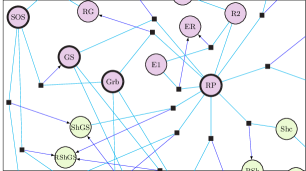
We apply the projection method to a model for the signalling network of epidermal growth factor receptor (EGFR) developed by Kholodenko et al. [2], see Figure 8.

4.1 Setup of EGFR model for application of projection technique

Figure 8: Factor graph of EGFR network as described in Kholodenko et al. [2] adapted to include enzyme reactions. Three added enzyme reactions with enzymes denoted E1-3 and enzyme-substrate complexes “enzyme-R” (denoted ER), “enzyme-PLC$\gamma$” (denoted EP), “enzyme-Shc” (denoted ES) are also shown to capture Michaelis-Menten contributions to the dynamics. The purple nodes denote subnetwork species while the bulk species are shown in green. See A for a full list of abbreviations for each network component.

We use the mass action rate parameters from [2]. Most of these fit directly into our setup of unary and binary reactions. The network also involves three Michaelis-Menten reactions transforming a “substrate” into a “product”. We incorporate these by adding to the description one enzyme and one enzyme-substrate complex species per reaction, with the rates for formation and dissociation of the complex large enough in order to force the two added species to be in equilibrium at any time with the prevailing substrate and product concentrations [36]. Initial conditions for the added species are then also derived from those of the substrate according to this equilibrium criterion. We choose the above method of incorporating Michaelis-Menten reactions as it allows direct application of the framework developed so far. We will report separately on an alternative approach where the enzyme reactions do not need to be represented explicitly.

To apply the projection method we need to first select a subnetwork and bulk from the EGFR network. We have chosen the bulk to be the protein Src homology and collagen domain protein (Shc) and any complexes that include Shc, consistent with our convention that if a protein is in the bulk, any complexes containing that protein will also be in the bulk. Shc and its complexes interact directly with four subnetwork species, which therefore form the boundary of our subnetwork; they are phosphorylated EGFR (denoted RP), growth factor receptor-binding protein 2 (Grb2, Son of Sevenless homolog protein (SOS), and protein complex Grb2-SOS (denoted GS; see A for a full list of abbreviations for network components). We then apply the projection method to obtain a set of equations for the subnetwork species. For the interior species these will have the original mass action form, while the boundary species will acquire additional memory (and random force) terms.

To avoid having to carry around concentration units in the following, we will switch to dimensionless concentrations defined as

$$\delta\tilde{x}_{i}=\delta x_{i}/y_{i}$$ (86)

Intuitively, the $\delta\tilde{x}_{i}$ are fractional concentration deviations from the steady state. The lowest value is $-1$, corresponding to a concentration of zero ($100\%$ below steady state), while e.g. $\delta\tilde{x}_{i}=2$ indicates that the concentration of $i$ is three times that in steady state.

The projected equations (12) written in terms of the dimensionless $\delta\tilde{x}_{i}$ take the form

$$\begin{split}\frac{\partial}{\partial t}\delta\tilde{x}_{i}&=\sum_{j=1}^{N^{\text{s}}}\delta\tilde{x}_{j}\tilde{\Omega}_{ji}^{\rm{s},\rm{s}}+\sum_{1\leq j\leq k\leq N^{\text{s}}}\delta\tilde{x}_{j}\delta\tilde{x}_{k}\tilde{\Omega}_{(jk)i}^{\rm{ss},\rm{s}}\\ &\quad+\int_{0}^{t}dt^{\prime}\left(\sum_{j=1}^{N^{\text{s}}}\delta\tilde{x}_{j}(t^{\prime})\tilde{M}_{ji}^{\rm{s},\rm{s}}(t-t^{\prime})+\sum_{1\leq j\leq k\leq N^{\text{s}}}\delta\tilde{x}_{j}(t^{\prime})\delta\tilde{x}_{k}(t^{\prime})\tilde{M}_{(jk)i}^{\rm{ss},\rm{s}}(t-t^{\prime})\right)+\tilde{r}_{i}(t)\end{split}$$ (87)

where

$$\begin{split}&\tilde{\Omega}_{ji}^{\rm{s},\rm{s}}=y_{j}\Omega_{ji}^{\rm{s},\rm{s}}y_{i}^{-1},\qquad\tilde{\Omega}_{(jk)i}^{\rm{ss},\rm{s}}=y_{j}y_{k}\Omega_{(jk)i}^{\rm{ss},\rm{s}}y_{i}^{-1},\\ \tilde{M}_{ji}^{\rm{s},\rm{s}}(t)=y_{j}M_{ji}^{\rm{s},\rm{s}}(t)y_{i}^{-1},&\qquad\tilde{M}_{(jk)i}^{\rm{ss},\rm{s}}(t)=y_{j}y_{k}M_{(jk)i}^{\rm{ss},\rm{s}}(t)y_{i}^{-1},\qquad\tilde{r}_{i}(t)=r_{i}(t)y_{i}^{-1}\end{split}$$ (88)

The rescaled rate matrix entries and random forces have dimensions of rate, i.e. inverse time, while the rescaled memory functions have dimensions of rate squared. The rate matrices and memory functions are calculated by first constructing the matrix $\bm{L}$ for the network, then using (58), (59), (63) and (67), and finally switching to dimensionless concentrations as explained above.

We will first discuss qualitative features of the memory functions themselves. Quantitative tests of the projected equations are presented next; as before, we will drop the random force terms so that the equations are a closed system determining the timecourses of the subnetwork concentrations for any given initial condition. To solve this numerically, we implement a solver for systems of integro-differential equations [37]. The enzyme reactions are much faster than the remainder of the kinetics and this causes the system of equations to become what is known as “stiff”. This can be handled by converting enzyme reaction terms in the subnetwork back into Michaelis-Menten form before using the numerical solver, or by transforming the projected equations into an enlarged set of differential equations [38]that can then be integrated using standard methods for stiff systems [39].

4.2 Memory function properties

We will now look at how general properties of the memory functions described in Section 3.3 manifest themselves in the EGFR network. We first analyse the amplitudes of the memory functions as in Section 3.3.2, to see how these reflect the structure of the network.

Figure 9 shows two of the linear memory functions in the equation of motion for the concentration of Grb2, one the self-memory and the other the cross-memory that determines the influence of past concentration values of SOS. The amplitudes are given by the intercepts with the $y$-axis ($\Delta t=0$): one sees that the self-amplitude of Grb2 is positive. To understand why, we note that Grb2 has two different reactions with bulk species:

$$\begin{split}\text{Grb2}+\text{ShP}&\leftrightharpoons\text{ShG}\\ \text{Grb2}+\text{RShP}&\leftrightharpoons\text{RShG}\end{split}$$ (89)

As these do not overlap, each reaction gives separate contributions to the self-memory amplitude of the form shown in Figs. 6a and 6b, which are always positive.

Figure 9: Memory functions in EGFR network: coefficients of Grb2 and SOS in the linear memory term for Grb2. The self memory function of Grb2 is compared to the contribution coming only from the reaction with phosphorylated Shc (ShP) as source and receiver channel. Contributions from other channels are no larger than $8\cdot 10^{-4}$s^-2.

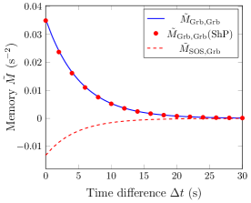
The amplitude of the cross-memory of $\delta\tilde{x}_{\text{GRB}}$ to $\delta\tilde{x}_{\text{SOS}}$, on the other hand, is negative as Figure 9 shows. To rationalise this, note that there are two bulk species that are shared between the bulk reactions of SOS and Grb2, namely ShG (ShP-Grb2) and RShGS (RShG-SOS/ShGS-RP). The reaction patterns involving these species both have the structure of Fig. 7d, and hence both give negative contributions.

Next we look at the time-dependence of the memory functions, and in particular the channel decomposition described in Sec. 3.3.3. For the self-memory of Grb2, there are two source and receiver channels, namely the two bulk reactions (89). The memory function can be decomposed into four pieces according to the combination of these four channels, e.g. “out via ShP (source) and in via RShP (receiver)”. It turns out in this case that the channel via phosphorylated Shc (ShP) dominates entirely. This is shown in Fig. 9, which compares the total memory function with its “out and in via ShP” contribution.

Note that the rates for both reactions (89) between Grb2 and the bulk are the same; however the steady state concentration of phosphorylated Shc (ShP) is much larger than the steady state value of RShP and therefore the reaction between Grb2 and phosphorylated Shc (ShP) to make ShP-Grb2 (ShG) is the one that dominates the self memory function of Grb2. Therefore it may be useful to study interactions between Shc and Grb2 to help understand why this reaction dominates the memory.

For the self-memory of phosphorylated EGFR (RP), which has four interactions with the bulk, the channel decomposition is richer because there are now 16 combinations of the four source and receiver channels. None of the $k^{+}_{sb,{c}}y_{b}$ values for the interactions with the bulk proteins is large enough to be entirely dominant and accordingly there are several channel combinations that give significant contributions to the memory. Fig. 10 shows the four that are largest: in and out via Shc; in and out via ShP; and in via Shc and out via ShP and vice versa. The combination of these gives a good account of the overall shape of the memory function, indicating that two channels (Shc and phosphorylated Shc (ShP)) are dominant over the other two (ShP-Grb2 (ShG) and ShGS (Shc-Grb2-SOS)). Looking at the figure closely one sees that the cross-channel contribution between Shc and ShP is positive for short time differences but becomes negative (and small) for longer time differences. In contrast the two other terms, for which the source and receiver channel is the same, are always positive.

Figure 10: Comparison of self memory function of phosphorylated EGFR (RP) with dominant terms from the channel decomposition: in and out via Shc; in and out via phosphorylated Shc (ShP); and in via Shc and out via phosphorylated Shc (ShP) and vice versa, shown together.

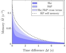
An analogous channel decomposition can be performed for (linear) cross memory and nonlinear memory functions as explained in Sec. 3.3.3. As for the linear self memory functions above, we find that often only a few channels provide the dominant contribution. This occurs for all the memory functions of EGFR. Fig. 11 shows that the nonlinear self memory of Grb2 is dominated by the reaction Grb2 + ShP $\rightarrow$ ShG acting as source and receiver, i.e. by the channel combination “in and out via phosphorylated Shc (ShP)”. This is not unexpected as the same combination dominates the linear self memory (see Fig. 9).

Figure 11: Comparison of nonlinear self memory function of Grb2 with the contribution from the channel combination “in and out via phosphorylated Shc (ShP)”.

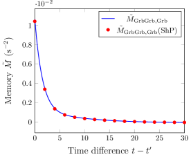
The channel decomposition can also be used to analyse self memory function timescales $\tau_{s}$ as defined in (83). In particular, if there is a single channel that dominates the memory function then the memory function contribution from this channel will have a similar timescale to the full memory function. For example, we find that the self memory of Grb2 has a timescale $\tau_{\text{Grb}}=5.31\,{\rm s}$. The contribution from the phosphorylated Shc (ShP) channel as source and receiver, shown in Fig. 9, has a timescale that is very close to this, namely $5.25\,{\rm s}$.

The memory function of phosphorylated EGFR (RP) has a faster timescale, $\tau_{\text{RP}}=1.68\,{\rm s}$. The contributions to the memory function which come from the “in and out via Shc” and “in and out via phosphorylated Shc (ShP)” channel combinations, on the other hand, have timescales of $1.08\,{\rm s}$ and $2.86\,{\rm s}$, respectively. The timescales of the contributions from the dominant channels are therefore sufficient to give an order-of-magnitude estimate of the overall memory function timescale.

The dominance of certain channels encourages us to look at how the system behaves if species or reactions that do not appear to contribute to the behaviour of the system are removed. The reaction between Grb2 and RShP does not make a significant contribution to the memory functions of Grb2. Excluding this reaction does not cause many changes to most of the memory functions involving Grb2, but some memory functions including $\tilde{M}_{\text{RP},\text{Grb}}$ have large differences. The change in $\tilde{M}_{\text{RP},\text{Grb}}$ occurs because removing the reaction between Grb2 and RShP means that phosphorylated EGFR (RP) and Grb2 only share interactions through phosphorylated Shc (ShP) and ShP-Grb2 (ShG). On the other hand, the channel decomposition shows that “in via Shc and out via RP-Shc-Grb2 (RShG)” and “in via phosphorylated Shc (ShP) and out via RP-Shc-Grb2 (RShG)” are the dominant reactions in this memory function and therefore removing this connection between phosphorylated EGFR (RP) and Grb2 will have a large effect on the memory behaviour. Therefore because all the channels are connected one cannot necessarily remove channels that look weak in one memory function, as this will generally have an effect on the other species.

One benefit of our analysis is that we can characterise explicitly also the nonlinear memory functions, and in particular assess the relative size of their contribution compared to the linear memory terms. Figure 12 shows the nonlinear self memory functions of the boundary species and Table 1 lists the amplitudes and timescales of the linear and nonlinear self memory functions. It is easy to see that the nonlinear self memory amplitudes are all smaller than their respective linear amplitudes. Similarly the nonlinear self memory functions decay faster than their respective linear contributions as shown by their shorter timescales. This suggests that, where it is desirable to capture nonlinear memory terms only approximately, relatively simple approximations like short-timescale exponentials could be considered. The nonlinear self memory of RP is a special case: the memory function changes sign (see Fig. 12) and the positive and negative contributions to the integral defining the timescale (see Sec. 3.3.3) cancel almost exactly, giving a notional timescale that is much shorter than for the other boundary species.

There are at least two ways one could use information from the memory functions to estimate the values of the dimensionless concentrations where nonlinearities become important. Concentrating on the self memory functions as above, the linear and nonlinear instantaneous (small $\Delta t$) contributions become comparable when $\tilde{M}^{\rm{s},\rm{s}}(0)\delta\tilde{x}_{s}=\tilde{M}^{\rm{ss},\rm{s}}(0)\delta\tilde{x}_{s}^{2}$, leading to the estimate $\delta\tilde{x}_{s}^{\rm c,1}=\tilde{M}^{\rm{s},\rm{s}}(0)/\tilde{M}^{\rm{ss},\rm{s}}(0)$ for the size of the linear regime. More relevant for the long-time dynamics is to consider the total memory terms assuming constant $\delta\tilde{x}_{s}(t)$. Then $\delta\tilde{x}_{s}^{\rm c,2}=\int_{0}^{\infty}dt\,\tilde{M}^{\rm{s},\rm{s}}(t)/\int_{0}^{\infty}dt\,\tilde{M}^{\rm{ss},\rm{s}}(t)$ would delimit the extent of the linear regime, i.e. the ratio of amplitude times timescale for the linear and nonlinear self memory.

The two estimates $\delta\tilde{x}_{s}^{\rm c,1}$ and $\delta\tilde{x}_{s}^{\rm c,2}$ defined above are shown in Table 1 alongside the memory amplitudes and timescales. We see that e.g. for Grb2-SOS (GS) $\delta\tilde{x}^{\rm c,2}=29.92$ whereas for Grb2 $\delta\tilde{x}^{\rm c,2}=9.37$; this suggests that for Grb2 nonlinear memory functions have a larger effect. To confirm this, we have run numerical experiments on time courses starting in steady state except for a perturbation in one of the four boundary species (see Table 1). We then compared the time courses for this species as predicted from the projected equations with and without the nonlinear memory terms, respectively, measuring the deviation between them as in Eq. (91) below. We find that these deviations are ordered among the four species in inverse proportion to their $\delta\tilde{x}^{\rm c,2}$, i.e. the larger this measure of the size of the linear regime, the smaller the nonlinear memory effects. Among the three species other than phosphorylated EGFR (RP) we also find quantitatively that deviations observed for an initial perturbation $\delta\tilde{x}_{s}(0)$ chosen as some constant fraction (say 1%) of $\delta\tilde{x}^{\rm c,2}_{s}$ are of similar magnitude. This indicates that values of $\delta\tilde{x}^{\rm c,2}$ can give not just qualitative but also quantitative information. Our tests show it to be superior to $\delta\tilde{x}^{\rm c,1}$ in this regard. For phosphorylated EGFR (RP), where because of the small notional nonlinear self memory timescale the value of $\delta\tilde{x}_{s}^{\rm c,2}$ is unrealistically large, we find that it still retains qualitative significance: the deviations that we measure due to the omission of the nonlinear memory terms are the smallest (by a factor of 100 compared to the next largest) among the four species tested.

Figure 12: The nonlinear self memory functions of Grb2-SOS (GS), SOS, Grb2 and phosphorylated EGFR (RP).

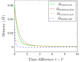
	linear		nonlinear		$\delta\tilde{x}_{s}^{\rm c,1}$	$\delta\tilde{x}_{s}^{\rm c,2}$
	amp.	$\tau$	amp.	$\tau$
RP	0.13	1.68	0.034	$-2.16\cdot 10^{-6}$	3.82	2.97$\cdot 10^{6}$
Grb2	0.036	5.31	0.01	2.04	3.6	9.37
SOS	0.12	4.61	0.056	0.82	2.14	12.05
GS	0.23	5.23	0.06	0.67	3.83	29.92

Table 1: The amplitudes (in s^-2) and timescales (in s) of linear and nonlinear self memory functions. Also shown are the estimates for the size of the linear regime resulting from instantaneous and long-time memory contributions, $\delta\tilde{x}_{s}^{\rm c,1}$ and $\delta\tilde{x}_{s}^{\rm c,2}$, respectively.

4.3 Changing the subnetwork

If we take the EGFR network and choose a different subnetwork then we will have a different set of boundary nodes and memory functions. Although the memory functions will be quantitatively different, their behaviour will still adhere to the general principles derived above. Let us take the EGFR network and change the subnetwork so that the bulk consists of Grb2 and all complexes that include Grb2. The boundary species of the subnetwork are now phosphorylated EGFR (RP), SOS, RShP and phosphorylated Shc (ShP). Figure 13 shows the linear self memory function of phosphorylated Shc (ShP) in the equation for ShP. ShP has two reactions with bulk species

$$\begin{split}\text{ShP}+\text{Grb2}&\leftrightharpoons\text{ShG}\\ \text{ShP}+\text{GS}&\leftrightharpoons\text{ShGS}\end{split}$$ (90)

As with the self memory function of Grb2 in Sec. 4.2 each reaction gives a separate positive contribution to the self-memory amplitude.

Figure 13: Comparison of self memory function of phosphorylated Shc (ShP) with dominant terms from the channel decomposition: in and out via Grb2; and in and out via Grb2-SOS (GS), shown together.

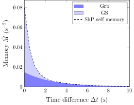
Next we consider the cross-species effects in the memory term for the evolution of ShP. The amplitude of the memory to past values of $\delta\tilde{x}_{\text{SOS}}$ is negative, whereas the amplitudes for memory to $\delta\tilde{x}_{\text{RP}}$ and $\delta\tilde{x}_{\text{RShP}}$ is positive, as shown in Fig. 14. This last amplitude is made up of two reaction patterns with the structure of Fig. 7b and hence has to be positive as we find. The cross memory functions of SOS and phosphorylated EGFR (RP) consist of a mixture of different reaction patterns from Fig. 7, and the sign of their amplitude is therefore determined by the relative sizes of the contributions of different signs. The amplitude of the cross memory function of SOS is negative, whereas the amplitude of the cross memory function of phosphorylated EGFR (RP) is positive but approximately ten times larger in size than the amplitude of the memory function for SOS.

Figure 14: Memory functions in EGFR network: coefficients of phosphorylated EGFR (RP), SOS and RShP in the linear memory term for phosphorylated Shc (ShP).

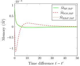
Also for the current changed subnetwork one can decompose the self memory functions into channels to understand the relative important of the latter. Fig. 13 shows that the two channels “out and in via Grb2” and “out and in via Grb2-SOS (GS)” both give similar contributions to the memory function of ShP. This is in line with the earlier analysis in Sec. 4.2: the $k^{+}_{sb,{c}}y_{b}$ values for both interactions are of the same order and therefore one would expect that neither channel will dominate the other.

Looking finally at the memory function timescales, the self memory function of phosphorylated Shc (ShP) has a timescale of $\tau_{\text{ShP}}=0.97$s. The “in and out via Grb2” and “in and out via Grb2-SOS (GS)” channels have timescales of 2.84s and 0.54s, respectively, and one sees that these can again be used to give an order of magnitude estimate of the full memory function timescale.

4.4 Quantitative tests

We conclude our discussion of the EGFR network by analysing the quantitative accuracy of the projected equations. As before we focus on the limit of low copy number noise ($\epsilon\to 0$) and drop the random force terms to have a closed description of the subnetwork dynamics. Our baseline is the solution of the full set of reaction equations for the entire network, consisting of both subnetwork and bulk. We compare the performance of the projected equations, including memory terms, to two simpler approximations without memory. In the first one we treat the subnetwork as isolated, i.e. all subnetwork-bulk reactions are ignored. In the second one we assume the bulk dynamics is fast enough for the bulk to be in steady state with respect to the specific subnetwork concentrations at any given time [18]. In practice, this means we solve the steady state conditions for the bulk concentrations at every time step and substitute them into the evolution equations for the subnetwork. All three approximation methods (projected equations without random force, isolated subnetwork, steady state bulk) come in two versions, one derived from the linearised dynamics and one for the full nonlinear dynamics.

Figure 15: Plots of time courses of some selected molecular species from the EGFR network. The fractional concentration deviations (86) are defined so that 0 represents steady state concentration, which is approached for long time, and $-1$ represents zero concentration. The solutions to the nonlinear projected equations are visually indistinguishable from those of the full reaction equations. Initial conditions were chosen as explained in the text.

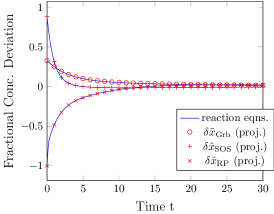
Figure 15 compares the solutions of the nonlinear projected equations to the baseline, the nonlinear reaction equations for the entire network. Time courses for phosphorylated EGFR (RP), Grb2 and SOS are shown. Here and in the following, the subnetwork initial conditions were chosen to maximise nonlinear effects: specifically we maximised $\sum_{s}[\delta\tilde{x}_{s}(0)]^{2}$ subject to the constraint that all conserved concentrations have the same value as at the steady state given by $\delta\tilde{x}_{i}=0$, and of course that all concentrations are non-negative ($\delta\tilde{x}_{s}(0)\geq-1$). The bulk was assumed to be in steady state initially, i.e. we set $\delta\tilde{x}_{b}(0)$ for all bulk species. As the figure shows, the agreement between the nonlinear projected equations and the full dynamics is excellent, with the two sets of time courses being visually indistinguishable.

Figure 16: Comparison of time courses obtained from full reaction equations with time courses for isolated subnetwork. Initial conditions chosen as in Fig. 15.

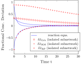
To demonstrate the importance of accounting for the interactions of the subnetwork with the bulk, we contrast in Fig. 16 the solutions for the isolated subnetwork to those of the full reaction equations: substantial differences appear, with the relaxation to steady state predicted to occur over a much larger timescale than in the full description.

The approximation of retaining information on the bulk network but assuming the bulk dynamics is fast would be expected to provide a more accurate description. This is borne out by Fig. 17, though deviations from the baseline are still larger than for the nonlinear projected equations, emphasizing the importance of keeping track of memory effects.

Figure 17: Comparison of time courses obtained from full reaction equations with time courses found by assuming the bulk dynamics is fast enough for the bulk to be at steady state. Initial conditions chosen as in Fig. 15.

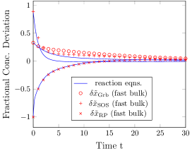
To develop a more quantitative picture of the performance of the various approximations for the subnetwork dynamics, we consider the same initial conditions as above but now scale down all the $\delta\tilde{x}_{s}(0)$ by a constant factor to tune the initial deviation of the subnetwork from steady state. The magnitude of this deviation will be quantified via the initial root mean squared deviation, $\delta=\{\sum_{s}[\delta\tilde{x}_{s}(0)]^{2}\}/N^{\text{s}}$, where $N^{\text{s}}$ is the number of subnetwork species as before. The accuracy of any approximation $\delta\hat{x}_{s}(t)$ for the subnetwork time courses will be measured by

$$\Delta=\frac{1}{T}\int_{0}^{T}dt^{\prime}\frac{1}{N^{\text{s}}}\sum_{s=1}^{N^{\text{s}}}\left|\delta\tilde{x}_{s}(t)-\delta\hat{x}_{s}(t)\right|$$ (91)

This is the absolute deviation in the dimensionless concentration of each subnetwork species, averaged over species and also a time interval $T$ that we choose as $T=150$s to capture the interesting transient regime, i.e. the approach to the steady state.

Figure 18: Plot of approximation error vs initial deviation from steady state in log-log representation, for three approximation methods derived from the linearised dynamics: linear projected equations, i.e. incorporating memory terms; steady state bulk approximation, i.e. without memory; and isolated subnetwork approximation. Dotted line is proportional to $\delta^{2}$ to demonstrate that the approximation error of the linear projected equations is only quadratic in $\delta$.

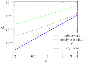
If we now consider first the linear projected equations and compare them to the full nonlinear reaction equations, we would expect the error to increase quadratically with the size $\delta$ of the initial deviations from steady state, at least for small $\delta$, because we are missing the nonlinear terms but are correctly capturing all linear terms including the memory. Fig. 18 verifies this expectation, showing that the average deviation $\Delta$ grows only as $\delta^{2}$. By contrast, the simpler approximations derived from the linearised dynamics, where we treat the subnetwork as isolated or the bulk as fast, should show deviations from the true time courses already at order $\delta$ because they neglect linear memory terms. Fig. 18 is consistent with this. It demonstrates in addition that the errors made by the memoryless approximations are substantially larger in absolute terms than for the projected equations. This demonstrates that memory terms are essential even to describe the linearised dynamics correctly.

Figure 19: Plot of approximation error vs initial deviation from steady state in log-log representation, for three approximation methods derived from the nonlinear dynamics: nonlinear projected equations, i.e. incorporating memory terms; steady state bulk approximation, i.e. without memory; and isolated subnetwork approximation. Dotted line is proportional to $\delta^{3}$ to demonstrate that the approximation error of the nonlinear projected equations grows only cubically in $\delta$. The dashed blue line indicates the estimated size of the error in the projected equations in the region where it is too small for the given initial conditions to calculate accurately.

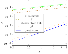
In Fig. 19 we show an analogous comparison for the nonlinear approximation methods. The memoryless approximations, isolated subnetwork and steady state bulk, still fail to catch memory contributions that are present already in the linearised dynamics, and accordingly give an approximation error that grows linearly in $\delta$. For the nonlinear projected equations, on the other hand, the approximation error comes only from the neglected random force terms. As explained in Section 3.2, when the bulk is initially in steady state then the random force will scale cubically with the initial deviations of the subnetwork from its steady state. One therefore expects an approximation error that is only of order $\delta^{3}$, and the results shown in Fig. 19 are consistent with this. Importantly, the figure shows also that the approximation error is very much smaller in absolute terms, by four orders of magnitude at the largest initial deviations from steady state and more for smaller $\delta$. We regard this as conclusive evidence that a quantitative description of subnetwork dynamics must include memory terms. The significant reduction in error over the linear projected equations, cf. Fig. 18, also emphasises that for quantitative accuracy nonlinearities in the memory have to be accounted for. By contrast, the memoryless approximations are hardly improved by the inclusion of nonlinear terms, which tells us that memory effects are crucial to get right first.

5 Discussion

We considered the problem of finding reduced descriptions for the dynamics of biological subnetworks embedded in a larger bulk environment. As an example we studied a subnetwork, embedded in the Shc-centred bulk, of an EGFR signalling model. Large-scale screens have identified collections of network components: interacting proteins [40] or genes regulated in response to a perturbation or disease state [41, 42], for example. The emergence of high-throughput functional imaging screens is providing further insights into potential signalling components, with direct or indirect consequences for signalling regulation and its alteration in disease states [43, 44]. In the absence of mechanistic details, however, there remains the problem of understanding the dynamics of a small subnetwork of interest in the presence of a surrounding network. While it is widely acknowledged that the presence of a surrounding bulk systems generates extrinsic noise on the subnetwork dynamics [6, 7], we showed that in addition one has memory effects whereby the state of the subnetwork in the past affects its time evolution in the present. We analysed these memory effects for a broad class of protein interaction networks containing unary and binary reactions, but argued that they should be much more generic.

Mathematically, our approach employed the projection method. This allows one to obtain a set of dynamical equations for the concentration of molecular species in a chosen subnetwork that forms part of a larger protein interaction network. These projected equations are closed, provided one neglects so-called random noise terms that contain the extrinsic noise as well as contributions from intrinsic noise. For the linearised dynamics, the projection method gives results that are fully consistent with an explicit elimination of the bulk variables. Non-trivially, we were able to apply the projection method also to the full nonlinear dynamics, where in the limit of low copy number noise we found explicit formulas for the memory functions. These memory functions provide the weights, as a function of the time difference, with which past subnetwork states affect the present time evolution. We showed that they can be calculated from appropriate matrix representations of the dynamical (Fokker-Planck) and projection operators.

We analysed in some detail the properties of the linear and nonlinear memory functions, including their amplitudes and timescales. These provide insights into how the subnetwork interacts with the bulk, with e.g. negative memory amplitudes requiring the existence of ternary subnetwork-bulk-bulk or subnetwork-subnetwork-bulk complexes.

In the final results section we applied the projection method to the EGFR network of Kholodenko et al. [2]. Here we illustrated how memory function amplitudes relate to subnetwork-bulk interaction structures. To understand memory function timescales, we used a channel decomposition. This is based on the fact that memory is generated by the past subnetwork state first affecting the bulk and then feeding back to the subnetwork at some later time. We showed that accordingly each memory function can be viewed as a sum of contributions from the different “source” and “receiver” channels in this feedback process. This allows one to identify which channels dominate the memory effects. The interpretation of each dominant channel can now be explored by designing experimentally tractable studies to interrogate parts of the subnetwork.

We also gave a quantitative comparison of the accuracy of the projected equations versus simpler memoryless approximations. This showed that including nonlinear terms in the memoryless approximations does little to reduce approximation error, because the main error comes from neglecting linear memory terms. The nonlinear projected equations, on the other hand, were significantly more accurate than other approximations, by at least four orders of magnitude compared to the nearest memoryless competitor.

While our analysis was focussed on memory functions, the projection approach can also capture noise effects, via the random force terms. In the low copy number noise limit, these terms represent directly the extrinsic noise on the subnetwork. We plan to report separately on the statistical properties of this extrinsic noise. The advantage of our approach here is that we can derive the extrinsic noise statistics, including e.g. temporal correlations, from the statistics of the initial states of the bulk, rather than having to postulate them separately. This will make it possible to test assumptions about extrinsic noise that have been made in the extensive literature on this subject, see e.g. [45].

The single-peaked steady state distribution $P_{\rm ss}$ that we considered means we do not explicitly treat systems with limit cycles or multiple states. However, if we allow more general distributions for $P_{\rm ss}$ we would be able to consider systems with these properties. The quantitative nature of the random force would be affected by this as “randomness” is always measured with respect to the assumed $P_{\rm ss}$.

Another area we are currently exploring is perturbations of the protein interaction dynamics, e.g. via gene regulation. Here one can ask, for example, what effect the perturbation of a bulk species has on the dynamics of the subnetwork [9]. This will allow us to study how regulation-driven changes in the concentration of bulk species such as partial or complete knockdowns affect the subnetwork.

In future work we also hope to address the inverse problem of how subnetwork dynamics can be used to infer information about the structure of an unknown bulk network. We saw that memory terms appear only in the time evolution of molecular species that lie on the boundary of the subnetwork, in the sense that they have direct interactions with the bulk. This can in principle be turned around immediately, so that by measuring memory functions from dynamics [46] one could identify which molecular species in a given subnetwork form its boundary. The next level would then involve identifying the network structure of the reactions with the bulk that these boundary species take part in. This would be a first step towards understanding the role of the many components which may be contained in a surrounding network, such as those identified by high-throughput functional screens [43], in coordinating a signalling response.

Appendix A Protein species Table

EGF	Epidermal Growth Factor
R	Extracellular domain of the monomeric EGFR
R${}_{\text{a}}$	EGF-EGFR complex
R2	(EGF-EGFR)/(EGF-EGFR) dimer also known as Ra:Ra dimer
RP	Tyrosine phosphorylated EGFR
PLC$\gamma$	Phospholipase C$\gamma$
Grb	Growth factor receptor-binding protein 2 (Grb2)
Shc	Src homology and collagen domain protein
SOS	Son of Sevenless homolog protein
E1	Enzyme for MM reaction between R2 and RP
ER	Enzyme complex for MM reaction between R2 and RP
E2	Enzyme for MM reaction between PLC$\gamma$ and PLC$\gamma$P
EP	Enzyme complex for MM reaction between PLC$\gamma$ and PLC$\gamma$P
E3	Enzyme for MM reaction between Shc and ShP
ES	Enzyme complex for MM reaction between Shc and ShP
RPL	RP-PLC$\gamma$
RPLP	RP-PLC$\gamma$P/ Phosphorylated RPL
RG	RP-Grb2
RGS	RP-Grb2-SOS
RSh	RP-Shc
RShP	RP-ShP/ Phosphorylated RSh
RShG	RP-Shc-Grb2
RShGS	RP-Shc-Grb2-SOS
GS	Grb2-SOS
ShP	Phosphorylated Shc
ShG	ShP-Grb2
ShGS	Shc-Grb2-SOS
PLC$\gamma$P	Phosphorylated PLC$\gamma$
PLC$\gamma$PI	PLC$\gamma$P translocated to membrane structures

Table 2: Abbreviations used for EGFR network components following Kholodenko et al. [2], including a description of each enzyme added to the system to account for the Michaelis Menten (MM) reactions.

References

- Bhalla [2003] U. S. Bhalla, Understanding complex signaling networks through models and metaphors, Prog. Biophys. Mol. Bio. 81 (2003) 45–65.
- Kholodenko et al. [1999] B. N. Kholodenko, O. V. Demin, G. Moehren, J. B. Hoek, Quantification of short term signaling by the epidermal growth factor receptor, The J. of Bio. Chem. 274 (1999) 30169–30181.
- Ackermann et al. [2012] J. Ackermann, J. Einloft, J. Nöthen, I. Koch, Reduction techniques for network validation in systems biology, J. Theor. Biol. 315 (2012) 71–80.
- Conradi et al. [2007] C. Conradi, D. Flockerzi, J. Raisch, J. Stelling, Subnetwork analysis reveals dynamic features of complex (bio)chemical networks, Proc. Natl. Acad. Sci. U. S. A. 104 (2007) 19175–19180.
- Shojaie and Michailidis [2010] A. Shojaie, G. Michailidis, Penalized principal component regression on graphs for analysis of subnetworks, in: Adv. Neur. In., 2010, pp. 2155–2163. Editor: J. Lafferty and C. K. I. Williams and J. Shawe-Taylor and R.S. Zemel and A. Culotta.
- Swain et al. [2002] P. S. Swain, M. B. Elowitz, E. D. Siggia, Intrinsic and extrinsic contributions to stochasticity in gene expression, Proc. Natl. Acad. Sci. U. S. A. 99 (2002) 12795–12800.
- Paulsson [2004] J. Paulsson, Summing up the noise in gene networks, Nature 427 (2004) 415–418.
- Normanno et al. [2006] N. Normanno, A. D. Luca, C. Bianco, L. Strizzi, M. Mancino, M. R. Maiello, A. Carotenuto, G. D. Feo, F. Caponigro, D. S. Salomon, Epidermal growth factor receptor (egfr) signaling in cancer, Gene 366 (2006) 2 – 16.
- Rubin and Sollich [2014] K. Rubin, P. Sollich, Perturbations in protein interaction networks, 2014. In preparation.
- Birtwistle et al. [2007] M. R. Birtwistle, M. Hatakeyama, N. Yumoto, B. A. Ogunnaike, J. B. Hoek, B. N. Kholodenko, Ligand-dependent responses of the erbb signaling network: experimental and modeling analyses, Mol Syst Biol 3 (2007) 144.
- Okino and Mavrovouniotis [1998] M. S. Okino, M. L. Mavrovouniotis, Simplification of mathematical models of chemical reaction systems, Chem. Rev. 98 (1998) 391–408.
- Radulescu et al. [2012] O. Radulescu, A. N. Gorban, A. Zinovyev, V. Noel, Reduction of dynamical biochemical reactions networks in computational biology, Front. Genet. 3 (2012) 131.
- Huang et al. [2010] Z. J. Huang, Y. Chu, J. Hahn, Model simplification procedure for signal transduction pathway models: An application to il-6 signaling, Chem. Eng. Sci. 65 (2010) 1964–1975.
- Gardiner [1984] C. W. Gardiner, Adiabatic elimination in stochastic-systems .1. Formulation of methods and application to few-variable systems, Phys. Rev. A 29 (1984) 2814–2822.
- Thomas et al. [2012] P. Thomas, R. Grima, A. V. Straube, Rigorous elimination of fast stochastic variables from the linear noise approximation using projection operators, Phys. Rev. E 86 (2012) 041110.
- Hartwell et al. [1999] L. H. Hartwell, J. J. Hopfield, S. Leibler, A. W. Murray, From molecular to modular cell biology, Nature 402 (1999) C47–C52.
- Conzelmann et al. [2004] H. Conzelmann, J. Saez-Rodriguez, T. Sauter, E. Bullinger, F. Allgower, E. D. Gilles, Reduction of mathematical models of signal transduction networks: simulation-based approach applied to egf receptor signalling, IEE Systems Biology 1 (2004) 159–69.
- Sunnaker et al. [2011] M. Sunnaker, G. Cedersund, M. Jirstrand, A method for zooming of nonlinear models of biochemical systems, BMC Syst. Biol. 5 (2011) 140.
- Liebermeister et al. [2005] W. Liebermeister, U. Baur, E. Klipp, Biochemical network models simplified by balanced truncation, FEBS J. 272 (2005) 4034–4043.
- Apri et al. [2012] M. Apri, M. de Gee, J. Molenaar, Complexity reduction preserving dynamical behavior of biochemical networks, J. Theor. Biol. 304 (2012) 16 – 26.
- Coolen and Rabello [2009] A. C. C. Coolen, S. Rabello, Generating functional analysis of complex formation and dissociation in large protein interaction networks, International Workshop On Statistical-mechanical Informatics 2009 (iw-smi 2009) 197 (2009) 012006.
- Mori [1965] H. Mori, Transport collective motion and brownian motion, Prog. Theor. Phys. 33 (1965) 423.
- Gardiner [2009] C. W. Gardiner, Stochastic methods: a handbook for the natural and social sciences, Springer Series in Synergetics, Springer-Verlag, Berlin, 4th edition edition, 2009.
- van Kampen [2007] N. G. van Kampen, Stochastic Processes in Physics and Chemistry, Elseiver, London, 3rd edition, 2007.
- Elf and Ehrenberg [2003] J. Elf, M. Ehrenberg, Fast evaluation of fluctuations in biochemical networks with the linear noise approximation, Genome Res 13 (2003) 2475–2484.
- Grima et al. [2011] R. Grima, P. Thomas, A. V. Straube, How accurate are the nonlinear chemical Fokker-Planck and chemical Langevin equations?, J. Chem. Phys. 135 (2011) 084103.
- Gillespie [2000] D. T. Gillespie, The chemical Langevin equation, J. Chem. Phys. 113 (2000) 297–306.
- Ritort and Sollich [2003] F. Ritort, P. Sollich, Glassy dynamics of kinetically constrained models, Adv. Phys. 52 (2003) 219–342.
- Hansen and McDonald [1990] J. P. Hansen, I. R. McDonald, Theory of Simple Liquids, Academic Press, 2nd edition, 1990.
- Götze [1991] W. Götze, Aspects of structural glass transitions, in: J. P. Hansen, D. Levesque, J. Zinn-Justin (Eds.), Liquids, freezing and glass transition, North-Holland, Amsterdam, 1991, pp. 287–503.
- Götze and Sjögren [1995] W. Götze, L. Sjögren, The mode coupling theory of structural relaxations, Transp. Theory Stat. Phys. 24 (1995) 801–853.
- Beck et al. [2011] M. Beck, A. Schmidt, J. Malmstroem, M. Claassen, A. Ori, A. Szymborska, F. Herzog, O. Rinner, J. Ellenberg, R. Aebersold, The quantitative proteome of a human cell line, Mol Syst Biol 7 (2011) 549.
- Nagaraj et al. [2011] N. Nagaraj, J. R. Wisniewski, T. Geiger, J. Cox, M. Kircher, J. Kelso, S. Paeaebo, M. Mann, Deep proteome and transcriptome mapping of a human cancer cell line, Mol Syst Biol 7 (2011) 548.
- Klipp et al. [2009] E. Klipp, W. Liebermeister, C. Wierling, A. Kowald, H. Lehrach, R. Herwig, Systems Biology: A Textbook, Wiley-VCH, 2009.
- Wick [1950] G. C. Wick, The evaluation of the collision matrix, Phys. Rev. 80 (1950) 268–272.
- Murray [2001] J. Murray, Mathematical Biology I. An Introduction, Springer, 2001.
- Day [1967] J. T. Day, Note on numerical solution of integro-differential equations, Comput. J. 9 (1967) 394.
- Rubin [2014] K. Rubin, Ph.D. thesis, King’s College London, 2014.
- Hairer and Wanner [1996] E. Hairer, G. Wanner, Solving ordinary differential equations II. Stiff and differential-algebraic problems, Springer Berlin Heidelberg, 2nd rev. edition, 1996.
- Kerrien et al. [2012] S. Kerrien, B. Aranda, L. Breuza, A. Bridge, F. Broackes-Carter, C. Chen, M. Duesbury, M. Dumousseau, M. Feuermann, U. Hinz, C. Jandrasits, R. C. Jimenez, J. Khadake, U. Mahadevan, P. Masson, I. Pedruzzi, E. Pfeiffenberger, P. Porras, A. Raghunath, B. Roechert, S. Orchard, H. Hermjakob, The intact molecular interaction database in 2012, Nucleic Acids Res. 40 (2012) D841–D846.
- Culhane et al. [2012] A. C. Culhane, M. S. Schroeder, R. Sultana, S. C. Picard, E. N. Martinelli, C. Kelly, B. Haibe-Kains, M. Kapushesky, A.-A. St Pierre, W. Flahive, K. C. Picard, D. Gusenleitner, G. Papenhausen, N. O’Connor, M. Correll, J. Quackenbush, Genesigdb: a manually curated database and resource for analysis of gene expression signatures, Nucleic Acids Res. 40 (2012) D1060–D1066.
- Sotiriou and Pusztai [2009] C. Sotiriou, L. Pusztai, Gene-expression signatures in breast cancer, New England Journal of Medicine 360 (2009) 790–800. PMID: 19228622.
- Fruhwirth et al. [2011] G. O. Fruhwirth, L. P. Fernandes, G. Weitsman, G. Patel, M. Kelleher, K. Lawler, A. Brock, S. P. Poland, D. R. Matthews, G. Keri, P. R. Barber, B. Vojnovic, S. M. Ameer-Beg, A. C. C. Coolen, F. Fraternali, T. Ng, How forster resonance energy transfer imaging improves the understanding of protein interaction networks in cancer biology, Chemphyschem 12 (2011) 442–461.
- Carlin et al. [2011] L. M. Carlin, R. Evans, H. Milewicz, L. Fernandes, D. R. Matthews, M. Perani, J. Levitt, M. D. Keppler, J. Monypenny, T. Coolen, P. R. Barber, B. Vojnovic, K. Suhling, F. Fraternali, S. Ameer-Beg, P. J. Parker, N. S. B. Thomas, T. Ng, A targeted sirna screen identifies regulators of cdc42 activity at the natural killer cell immunological synapse, Science Signaling 4 (2011) ra81.
- Shahrezaei et al. [2008] V. Shahrezaei, J. F. Ollivier, P. S. Swain, Colored extrinsic fluctuations and stochastic gene expression, Mol Syst Biol 4 (2008) 196.
- Uranagase and Munakata [2010] M. Uranagase, T. Munakata, Generalized Langevin equation revisited: mechanical random force and self-consistent structure, J. Phys. A 43 (2010) 455003.