1. Introduction

1.1. Problem formulation

Consider time-harmonic waves propagating in a medium where the wave speed varies smoothly, but is constant outside of a bounded domain $\Omega\subset\mathbb{R}^{2}$. This manuscript presents a technique for numerically solving the scattering problem in such a medium. Specifically, we seek to compute the scattered wave $u^{\mbox{\tiny s}}$ that results when a given incident wave $u^{\mbox{\tiny i}}$ (which satisfies the free space Helmholtz equation) impinges upon the region with variable wave speed, as in Figure 1. Mathematically, the scattered field $u^{\mbox{\tiny s}}$ satisfies the variable coefficient Helmholtz equation

(1) $$\Delta u^{\mbox{\tiny s}}(\bm{x})+\kappa^{2}(1-b(\bm{x}))u^{\mbox{\tiny s}}(\bm{x})=\kappa^{2}b(\bm{x})u^{\mbox{\tiny i}}(\bm{x}),\qquad\bm{x}\in\mathbb{R}^{2},$$

and the outgoing Sommerfeld radiation condition

(2) $$\frac{\partial u^{\mbox{\tiny s}}}{\partial r}-i\kappa u^{\mbox{\tiny s}}=o(r^{-1/2}),\qquad r:=|\bm{x}|\to\infty,$$

uniformly in angle. The real number $\kappa$ in (1) and (2) is the free space wavenumber (or frequency), and the so called “scattering potential” $b=b(\bm{x})$ is a given smooth function that specifies how the wave speed (phase velocity) $v(\bm{x})$ at the point $\bm{x}\in\mathbb{R}^{2}$ deviates from the free space wave speed $v_{\rm free}$,

(3) $$b(\bm{x})=1-\left(\frac{v_{\rm free}}{v(\bm{x})}\right)^{2}.$$

One may interpret $\sqrt{1-b}$ as a spatially-varying refractive index. Observe that $b$ is identically zero outside $\Omega$. Together, equations (1) and (2) completely specify the problem. When $1-b(\bm{x})$ is real and positive for all $\bm{x}$, the problem is known to have a unique solution for each positive $\kappa$ [10, Thm. 8.7].

The transmission problem (1)-(2), and its generalizations, have applications in acoustics, electromagnetics, optics, and quantum mechanics. Some specific applications include underwater acoustics [3], ultrasound and microwave tomography [14, 35], wave propagation in metamaterials and photonic crystals, and seismology [36]. The solution technique in this paper is high-order accurate, robust and computationally highly efficient. It is based on a direct (as opposed to iterative) solver, and thus is particularly effective when the response of a given potential $b$ to multiple incident waves $u^{\mbox{\tiny i}}$ is desired, as arises in optical device characterization, or computing radar scattering cross-sections. The complexity of the method is $O(N^{3/2})$ where $N$ is the number of discretization points in $\Omega$. Additional solves with the same scattering potential $b$ and wavenumber $\kappa$ require only $O(N)$ operations. (Further reductions in asymptotic complexity can sometimes be attained; see section 4.2.) For simplicity of presentation, the solution technique is presented in $\mathbb{R}^{2}$; however, the method can be directly extended to $\mathbb{R}^{3}$.

Remark 1.1.

Equation (1) is derived by requiring that the total field $u=u^{\mbox{\tiny s}}+u^{\mbox{\tiny i}}$ satisfy the variable coefficient Helmholtz equation

(4) $$\Delta u(\bm{x})+\kappa^{2}\,\left(\frac{v_{\rm free}}{v(\bm{x})}\right)^{2}u(\bm{x})=0,\qquad\bm{x}\in\mathbb{R}^{2}.$$

Plugging the condition that the incident field $u^{\mbox{\tiny i}}$ satisfies the free space equation $(\Delta+\kappa^{2})u^{\mbox{\tiny i}}=0$ inside $\Omega$, and the definition of the scattering potential (3) into (4) results in (1).

Figure 1. Geometry of scattering problem. Waves propagate in a medium with constant wave speed $v_{\rm free}$ everywhere except in the shaded areas, where the wave speed is given by $v(\bm{x})=v_{\rm free}/\sqrt{1-b(\bm{x})}$ where $b=b(\bm{x})$ is a given, smooth, compactly supported “scattering potential.” An incident field $u^{\mbox{\tiny i}}$ hits the scattering potential and induces the scattered field $u^{\mbox{\tiny s}}$. The dashed line marks the artificial domain $\Omega$ which encloses the support of the scattering potential.

1.2. Outline of proposed method

We solve (1)-(2) by splitting the problem into two parts, namely a variable-coefficient problem on the bounded domain $\Omega$, and a constant coefficient problem on the exterior domain $\Omega^{\rm c}:=\mathbb{R}^{2}\backslash\overline{\Omega}$. For each of the two domains, a solution operator in the form of a Dirichlet-to-Neumann (DtN) map on the boundary ${\partial\Omega}$ is constructed. These operators are then “glued” together on ${\partial\Omega}$ to form a solution operator for the full problem. The end result is a discretized boundary integral operator that takes as input the restriction of the incoming field $u^{\mbox{\tiny i}}$ (and its normal derivative) to $\partial\Omega$, and constructs the restriction of the scattered field $u^{\mbox{\tiny s}}$ on $\partial\Omega$ (and its normal derivative). Once these quantities are known, the total field can rapidly be computed at any point $\bm{x}\in\mathbb{R}^{2}$.

1.2.1. Solution technique for the variable-coefficient problem on $\Omega$

For the interior domain $\Omega$, we construct a solution operator for the following homogeneous variable-coefficient boundary value problem where the unknown total field $u=u^{\mbox{\tiny s}}+u^{\mbox{\tiny i}}$ satisfies

(5) $$\Delta u(\bm{x})+\kappa^{2}(1-b(\bm{x}))u(\bm{x})= \ 0, \bm{x} \in\Omega,$$

(6) $$u(\bm{x})= \ h(\bm{x}) \bm{x} \in{\partial\Omega}.$$

Note that, for now, we specify the Dirichlet data $h$; when we consider the full problem $h$ will become an unknown that will also be solved for. It is known that, for all but a countable set of wavenumbers, the interior Dirichlet BVP (5)-(6) has a unique solution $u$ [26, Thm. 4.10]. The values $\{\kappa_{j}\}_{j=1}^{\infty}$ at which the solution is not unique are (the square roots of) the interior Dirichlet eigenvalues of the penetrable domain $\Omega$; we will call them resonant wavenumbers.

Definition 1.1 (interior Dirichlet-to-Neumann map).

Suppose that $\kappa>0$ is not a resonant wavenumber of $\Omega$. Then the interior Dirichlet-to-Neumann (DtN) operator $T_{\rm int}:H^{1}({\partial\Omega})\to L^{2}({\partial\Omega})$ is defined by

(7) $$T_{\rm int}h=u_{n},$$

where $u$ the solution to (5)–(6) corresponding to Dirichlet data $h$, for any $h\in H^{1}({\partial\Omega})$.

Remark 1.2.

The operator $T_{\rm int}$ is a pseudo-differential operator of order $+1$ [15]; that is, in the limit of high-frequency boundary data it behaves like a differentiation operator on ${\partial\Omega}$. The boundedness as a map $T_{\rm int}:H^{1}({\partial\Omega})\to L^{2}({\partial\Omega})$ holds for $\Omega$ any bounded Lipschitz domain since the PDE is strongly elliptic [26, Thm. 4.25].

In this paper, a discrete approximation to $T_{\rm int}$ is constructed via a variation of recent composite spectral methods in [16, 25] (which are also similar to [9]). These methods partition $\Omega$ into a collection of small “leaf” boxes and construct approximate DtN operators for each box via a brute force calculation on a local spectral grid. The DtN operator for $\Omega$ is then constructed via a hierarchical merge process. Unfortunately, at any given $\kappa$, each of the many leaves and merging subdomains may hit a resonance as described above, causing its DtN to fail to exist. As $\kappa$ approaches any such resonance the norm of the DtN grows without bound. Thus a technique based on the DtN alone is not robust.

Remark 1.3.

We remind the reader that any such “box” resonance is purely artificial and is caused by the introduction of the solution regions. It is important to distinguish these from resonances that the physical scattering problem (1)-(2) itself might possess (e.g. due to nearly trapped rays), whose effect of course cannot be avoided in any accurate numerical method.

One contribution of the present work is to present a robust improvement to the methods of [16, 25], built upon hierarchical merges of impedance-to-impedance (ItI) rather than DtN operators; see section 2. The idea of using impedance coupling builds upon the work of Kirsch–Monk [22]. ItI operators are inherently stable, with condition number $O(1)$, and thus exclude the possibility of inverting arbitrarily ill-conditioned matrices as in the original DtN formulation. For instance, in the lens experiment of section 5, the DtN method has condition numbers as large as $2\times 10^{5}$, while for the new ItI method the condition number never grows larger than $20$. The DtN of the whole domain $\Omega$ is still needed; however, if $\Omega$ has a resonance, the size of $\Omega$ can be changed slightly to avoid the resonance (see remark 2.6).

The discretization methods in [16, 25], and in this paper are related to earlier work on spectral collocation methods on composite (“multi-domain”) grids, such as, e.g., [23, 39], and in particular Pfeiffer et al [29]. For a detailed review of the similarities and differences, see [25].

1.2.2. Solution technique for the constant coefficient problem on $\Omega^{\rm c}$

On the exterior domain, we build a solution operator for the constant coefficient problem

(8) $$\Delta u^{\mbox{\tiny s}}(\bm{x})+\kappa^{2}u^{\mbox{\tiny s}}(\bm{x})= \ 0, \bm{x}\in\Omega^{\rm c},$$

(9) $$u^{\mbox{\tiny s}}(\bm{x})= \ s(\bm{x}), \bm{x}\in\partial\Omega,$$

(10) $$\frac{\partial u^{\mbox{\tiny s}}}{\partial r}-i\kappa u^{\mbox{\tiny s}}= \ o(r^{-1/2}), r:=|{\mathbf{x}}|\to\infty,$$

obtained by restricting (1)-(2) to $\Omega^{\rm c}$. (Again, the Dirichlet data $s$ later will become an unknown that is solved for.) It is known that (8)-(10) has a unique solution for every wavenumber $\kappa$ [10, Ch. 3]. This means that the following DtN for the exterior domain is always well-defined.

Definition 1.2 (exterior Dirichlet-to-Neumann map).

Suppose that $\kappa>0$. The exterior DtN operator $T_{\rm ext}:H^{1}({\partial\Omega})\to L^{2}({\partial\Omega})$ is defined by

(11) $$T_{\rm ext}s=u^{\mbox{\tiny s}}_{n}$$

for $u^{\mbox{\tiny s}}$ the unique solution to the exterior Dirichlet BVP (8)-(10).

Numerically, we construct an approximation to $T_{\rm ext}$ by reformulating (8)-(10) as a boundary integral equation (BIE), as described in section 3.1, and then discretizing it using a Nyström method based on a high order Gaussian composite quadrature [19].

1.2.3. Combining the two solution operators

Once the DtN operators $T_{\rm int}$ and $T_{\rm ext}$ have been determined (as described in sections 1.2.1 and 1.2.2), and the restriction of the incident field to $\partial\Omega$ is given, it is possible to determine the scattered field on $\partial\Omega$ as follows. First observe that the total field $u=u^{\mbox{\tiny s}}+u^{\mbox{\tiny i}}$ must satisfy

(12) $$T_{\rm int}(u^{\mbox{\tiny i}}|_{\partial\Omega}+u^{\mbox{\tiny s}}|_{\partial\Omega})=u^{\mbox{\tiny i}}_{n}+u^{\mbox{\tiny s}}_{n}.$$

We also know that the scattered field $u^{\mbox{\tiny s}}$ satisfies

(13) $$T_{\rm ext}u^{\mbox{\tiny s}}|_{\partial\Omega}=u^{\mbox{\tiny s}}_{n}.$$

Combining (12) and (13) to eliminate $u^{\mbox{\tiny s}}_{n}$ results in the equation (analogous to [22, Eq. (2.12)]),

(14) $$(T_{\rm int}-T_{\rm ext})u^{\mbox{\tiny s}}|_{\partial\Omega}=u^{\mbox{\tiny i}}_{n}-T_{\rm int}u^{\mbox{\tiny i}}|_{\partial\Omega}.$$

As discussed in Remark 1.2, both $T_{\rm int}$ and $T_{\rm ext}$ have order $+1$. Lamentably, this behavior adds rather than cancels in (14), so that $(T_{\rm int}-T_{\rm ext})$ also has order $+1$, and is therefore unbounded. This makes any numerical discretization of (14) ill-conditioned, with condition number growing linearly in the number of boundary nodes. To remedy this, we present in section 3 a new method for combining $T_{\rm int}$ and $T_{\rm ext}$ to give a provably second kind integral equation, which thus gives a well-conditioned linear system.

Once the scattered field is known on the boundary, the field at any exterior point may be found via Green’s representation formula; see section 3.3. The interior transmitted wave $u$ may be reconstructed anywhere in $\Omega$ by applying solution operators which were built as part of the composite spectral method.

1.3. Prior work

Perhaps the most common technique for solving the scattering problem stated in Section 1.1 is to discretize the variable coefficient PDE (1) via a finite element or finite difference method, while approximating the radiation condition in one of many ways, including perfectly matched layers (PML) [20], absorbing boundary conditions (ABC) [12], separation of variables or their perturbations [27], local impedance conditions [7], or a Nyström method [22] (as in the present work). However, the accuracy of finite element and finite difference schemes for the Helmholtz equation is limited by so-called “pollution” (dispersion) error [2, 4], demanding an increasing number of degrees of freedom per wavelength in order to maintain fixed accuracy as wavenumber $\kappa$ grows. In addition, while the resulting linear system is sparse, it is also large and is often ill-conditioned in such a way that standard pre-conditioning techniques fail, although hybrid direct-iterative solvers such as [13] have proven effective in certain environments. While there do exist fast direct solvers for such linear systems (for low wavenumbers $\kappa$) [32, 31, 37, 24], the accuracy of the solution is limited by the discretization. The performance of the solver worsens when increasing the order of the discretization—thus it is not feasible to use a high order discretization that would overcome the above-mentioned pollution error.

Scattering problems on infinite domains are also commonly handled by rewriting them as volume integral equations (e.g. the Lippmann–Schwinger equation) defined on a domain (such as $\Omega$) that contains the support of the scattering potential [1, 8]. This approach is appealing in that the Sommerfeld condition (2) is enforced analytically, and in that high-order discretizations can be implemented without loss of stability [11]. Principal drawbacks are that the resulting linear systems have dense coefficient matrices, and tend to be challenging to solve using iterative solvers [11].

1.4. Outline

Section 2 describes in detail the stable hierarchical procedure for constructing an approximation to the DtN map $T_{\rm int}$ for the interior problem (5)-(6). Section 3 describes how boundary integral equation techniques are used to approximate the DtN map $T_{\rm ext}$ for the exterior problem (8)-(10), how to couple the DtN maps $T_{\rm int}$ and $T_{\rm ext}$ to solve the full problem (1)-(2), and the proof (Theorem 3.1) that the formulation is second kind. Section 4 details the computational cost of the method and explains the reduced cost for multiple incident waves. Finally, section 5 illustrates the performance of the method in several challenging scattering potential configurations.

2. Constructing and merging impedance-to-impedance maps

This section describes a technique for building a discrete approximation to the Dirichlet-to-Neumann (DtN) operator for the interior variable coefficient BVP (5)-(6) on a square domain $\Omega$. It relies on the hierarchical construction of impedance-to-impedance (ItI) maps; these are defined in section 2.1. Section 2.2 defines a hierarchical tree on the domain $\Omega$. Section 2.3 explains how the ItI maps are built on the (small) leaf boxes in the tree. Section 2.4 describes the merge procedure whereby the global ItI map is built, and then how the global DtN map is recovered from the global ItI map.

2.1. The impedance-to-impedance map

We start by defining the ItI map on a general Lipschitz domain, and giving some of its properties. (In this section only, $\Omega$ will refer to such a general domain.)

Proposition 2.1.

Let $\Omega\subset\mathbb{R}^{2}$ be a bounded Lipschitz domain, and $b(\bm{x})$ be real. Let $\eta\in\mathbb{C}$, and $\operatorname{Re}\eta\neq 0$. Then the interior Robin BVP,

(15) $$[\Delta+\kappa^{2}(1-b(\bm{x}))]u(\bm{x}) = 0\qquad\bm{x}\in\Omega~{},$$

(16) $$u_{n}+i\eta u|_{\partial\Omega} = f\qquad\mbox{ on }{\partial\Omega}~{},$$

has a unique solution $u$ for all real $\kappa>0$.

Proof.

We first prove uniqueness. Consider $u$ a solution to the homogeneous problem $f\equiv 0$. Then using Green’s 1st identity and (15), (16),

$$-i\eta\int_{\partial\Omega}|u|^{2}=\int_{\partial\Omega}\overline{u}u_{n}=\int_{\Omega}|\nabla u|^{2}-\kappa^{2}(1-b)|u|^{2}.$$

Taking the imaginary part shows that $u$, and hence $u_{n}$, vanishes on ${\partial\Omega}$, hence $u\equiv 0$ in $\Omega$ by unique continuation of the Cauchy data. Existence of $u\in H^{1}(\Omega)$ now follows for data $f\in H^{-1/2}({\partial\Omega})$ from the Fredholm alternative, as explained in this context by McLean [26, Thm. 4.11]. ∎

Definition 2.1 (interior impedance-to-impedance map).

Fix $\eta\in\mathbb{C}$, and $\operatorname{Re}\eta\neq 0$. Let

(17) $$f := u_{n}+i\eta u|_{\partial\Omega}$$

(18) $$g := u_{n}-i\eta u|_{\partial\Omega}$$

be Robin traces of $u$. We refer to $f$ and $g$ as the “incoming” and “outgoing” (respectively) impedance data. For any $\kappa>0$, the interior ItI operator $R:L^{2}({\partial\Omega})\to L^{2}({\partial\Omega})$ is defined by

(19) $$Rf=g$$

for $f$ and $g$ the Robin traces of $u$ the solution of (15)–(16), for all $f\in L^{2}({\partial\Omega})$.

We choose the impedance parameter $\eta$ (on dimensional grounds) to be $\eta=\kappa$. Numerically, in what follows, we observe very little sensitivity to the exact value or sign of $\eta$.

For the following, we need the result that the DtN map $T_{\rm int}$ is self-adjoint for real $\kappa$ and $b(\bm{x})$. This holds since, for any functions $u$ and $v$ satisfying $(\Delta+\kappa^{2}(1-b))u=0$ in $\Omega$ and $(\Delta+\kappa(1-b))v=0$ in $\Omega$,

$$0=\int_{\Omega}\overline{v}(\Delta+\omega^{2}(1-b))u-u(\Delta+\overline{\kappa^{2}(1-b)})\overline{v}=\int_{\partial\Omega}\overline{v}u_{n}-u\overline{v_{n}}\\ =(v|_{\partial\Omega},T_{\rm int}u|_{\partial\Omega})-(T_{\rm int}v|_{\partial\Omega},u|_{\partial\Omega})$$

by Green’s second identity. This allows us to prove the following property of the ItI map that will be the key to the numerical stability of the method.

Proposition 2.2.

Let $\Omega$ be a bounded Lipschitz domain, let $b(\bm{x})$ be real, and let $\eta\in\mathbb{C}$ and $\operatorname{Re}\eta\neq 0$. Then the ItI map $R$ for $\Omega$ exists for all real frequencies $\kappa$, and is unitary whenever $\eta$ is also real.

Proof.

Existence of $R$ for all real $\kappa$ follows from Proposition 2.1. To prove $R$ is unitary, we insert the definitions of $f$ and $g$ into (19) and use the definition of the DtN to rewrite $u_{n}=T_{\rm int}u|_{\partial\Omega}$, giving

(20) $$R(T_{\rm int}+i\eta)u|_{\partial\Omega}=(T_{\rm int}-i\eta)u|_{\partial\Omega}~{},$$

which holds for any data $u|_{\partial\Omega}\in H^{1}({\partial\Omega})$. Thus the ItI map is given in operator form by

(21) $$R=(T_{\rm int}-i\eta)(T_{\rm int}+i\eta)^{-1}~{}.$$

Since $T_{\rm int}$ is self-adjoint and $\eta$ is real, this formula shows that $R$ is unitary. ∎

As a unitary operator, $R$ has unit operator $L^{2}$-norm, pseudo-differential order $0$, and eigenvalues lying on the unit circle. From (21) and the pseudo-differential order of $T_{\rm int}$ one may see that the eigenvalues of $R$ accumulate only at $+1$.

Figure 2. The square domain $\Omega$ shown split hierarchically into boxes. The case where there are $4\times 4$ leaf boxes is shown, ie there are $M=2$ levels. These are then gathered into a binary tree of successively larger boxes as described in Section 2. One possible enumeration of the boxes in the tree is shown, but note that the only restriction is that if box $\tau$ is the parent of box $\sigma$, then $\tau<\sigma$.

Figure 3. (a) The set of $4q$ Gauss–Legendre points used to represent the ItI on the boundary of a leaf box $\Omega^{\tau}$. The case $q=14$ is shown. (b) Chebyshev discretization used for the PDE spectral solution on the same leaf box, for the case $p=16$. Interior nodes $J_{i}$ are shown by small black dots. The four sets of $p-1$ Chebyshev boundary nodes are shown (each a different color); each set includes the start corner (in counter-clockwise ordering) but not the end corner. The set of all Chebyshev boundary nodes is $J_{b}=[J_{s},\;J_{e},\;J_{n},\;J_{w}]$.

2.2. Partitioning of $\Omega$ into hierarchical tree of boxes

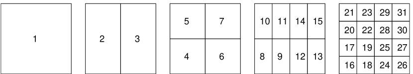
Recall that $\Omega$ is the square domain containing the support of $b$. We partition $\Omega$ into a collection of $4^{M}$ equally-sized square boxes called leaf boxes, where $M$ sets the number of levels; see Figure 2. We place $q$ Gauss–Legendre interpolation nodes on each edge of each leaf, which will serve to discretize all interactions of this leaf with its neighbors; see Figure 3(a). The size of the leaf boxes, and the parameter $q$, should be chosen so that any potential transmitted wave $u$, as well as its first derivatives, can be accurately interpolated on each box edge from their values at these nodes.

Next we construct a binary tree over the collection of leaf boxes. This is achieved by forming the union of adjacent pairs boxes (forming rectangular boxes), then forming the pairwise union of the rectangular boxes. The result is a collection of squares with twice the side length of a leaf box. The process is continued until the only box is $\Omega$ itself, as in Figure 2. The boxes should be ordered so that if $\tau$ is a parent of a box $\sigma$, then $\tau<\sigma$. We also assume that the root of the tree (i.e. the full box $\Omega$) has index $\tau=1$. Let $\Omega^{\tau}$ denote the domain associated with box $\tau$.

Remark 2.1.

The method easily generalizes to rectangular boxes, and to more complicated domains $\Omega$ in the same manner as [25].

2.3. Spectral approximation of the ItI map on a leaf box

Let $\Omega^{\tau}$ denote a single leaf box, and let $\bm{\mathsf{f}}=\bm{\mathsf{f}}^{\tau}$ and $\bm{\mathsf{g}}=\bm{\mathsf{g}}^{\tau}$ be a pair of vectors of associated incoming and outgoing impedance data, sampled at the $4q$ Gauss–Legendre boundary nodes, with entries ordered in a counter-clockwise fashion starting from the leftmost node of the bottom edge of the box, as in Figure 3(a). In this section, we describe a technique for constructing a matrix approximation to the ItI operator on this leaf box. Namely, we build a $4\,q\times 4\,q$ matrix $\bm{\mathsf{R}}$ such that

$$\bm{\mathsf{g}}\approx\bm{\mathsf{R}}\bm{\mathsf{f}}$$

holds to high-order accuracy, for all incoming data vectors $\bm{\mathsf{f}}\in\mathbb{R}^{4q}$ corresponding to smooth transmitted wave solutions $u$.

First, we discretize the PDE (15) on the square leaf box $\Omega^{\tau}$ using a spectral method on a $p\times p$ tensor product Chebyshev grid filling the box, as in Figure 3(b), comprised of the nodes at locations

$$\left(\frac{a+b}{2}+hx_{i},\;\frac{c+d}{2}+hx_{j}\right),\qquad i,j=1,\ldots,p$$

where $x_{j}:=\cos\left(\frac{\pi(j-1)}{p-1}\right)$, $j=1,\ldots,p$ are the Chebyshev points on $[-1,1]$. We label the Chebyshev node locations $\bm{x}_{j}\in\mathbb{R}^{2}$, for $j=1,\ldots,p^{2}$. For notational purposes, we order these nodes in the following fashion: the indices $J_{b}=\{1,2,\ldots,4(p-1)\}$ correspond to the Chebyshev nodes lying on the boundary of $\Omega^{\tau}$, ordered counter-clockwise starting from the node located at the south-west corner $(a,c)$. The remaining $(p-2)^{2}$ interior nodes have indices $J_{i}=\{4(p-1)+1,\ldots,p^{2}\}$ and may be ordered arbitrarily (a Cartesian ordering is convenient).

Let ${\bm{\mathsf{D}}^{(1)}},{\bm{\mathsf{D}}^{(2)}}\in\mathbb{R}^{p^{2}\times p^{2}}$ be the standard spectral differentiation matrices constructed on the full set of Chebyshev nodes, which approximate the $\partial/\partial x_{1}$ (horizontal) and $\partial/\partial x_{2}$ (vertical) derivative operators, respectively. As explained in [33, Ch. 7], these are constructed from Kronecker products of the $p\times p$ identity matrix and $h^{-1}\bm{\mathsf{D}}$, where $\bm{\mathsf{D}}\in\mathbb{R}^{p\times p}$ is the usual one-dimensional differentiation matrix on the nodes $\{x_{i}\}_{i=1}^{p}$. Namely $\bm{\mathsf{D}}$ has entries $\bm{\mathsf{D}}_{ij}=\frac{w_{j}}{w_{i}(x_{i}-x_{j})}$ where $\{w_{j}\}_{j=1}^{p}=[1/2,-1,1,-1,\ldots,(-1)^{p},(-1)^{p-1}/2]$ is the vector of barycentric weights for the Chebyshev nodes (see [33, Ch. 6] and [30, Eqn.(8)].) Let the matrix $\bm{\mathsf{A}}\in\mathbb{R}^{p^{2}\times p^{2}}$ be the spectral discretization of the operator $\Delta+\kappa^{2}(1-b({\mathbf{x}}))$ on the product Chebyshev grid, namely

$$\bm{\mathsf{A}}=({\bm{\mathsf{D}}^{(1)}})^{2}+({\bm{\mathsf{D}}^{(2)}})^{2}+\mbox{ diag }\{\kappa^{2}(1-b({\mathbf{x}}_{j}))\}_{j=1}^{p^{2}}~{},$$

where “diag S” indicates the diagonal matrix whose entries are the elements of the ordered set $S$.

Remark 2.2.

The matrices ${\bm{\mathsf{D}}^{(1)}}$, ${\bm{\mathsf{D}}^{(2)}}$, and $\bm{\mathsf{A}}$ must have rows and columns ordered as explained above (i.e. boundary then interior) for the Chebyshev nodes; this requires permuting rows and columns of the matrices constructed by Kronecker products. For example, the structure of $\bm{\mathsf{A}}$ is

$$\left[\begin{array}[]{ll}\bm{\mathsf{A}}_{bb}&\bm{\mathsf{A}}_{bi}\\ \bm{\mathsf{A}}_{ib}&\bm{\mathsf{A}}_{ii}\end{array}\right]~{},$$

where the notation $\bm{\mathsf{A}}_{bi}$ indicates the submatrix block $\bm{\mathsf{A}}(J_{b},J_{i})$, etc.

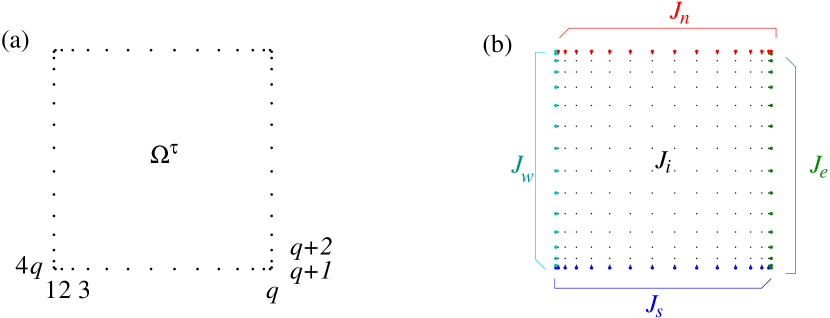
We now break the $4(p-1)$ boundary Chebyshev nodes into four sets $J_{b}=[J_{s},\;J_{e},\;J_{n},\;J_{w}]$, denoting the south, east, north, and west edges, as in Figure 3(b). Note that $J_{s}$ includes the south-western corner $J_{s}(1)$ but not the south-eastern corner (which in turn is the first element of $J_{e}$), etc.

We are now ready to derive the linear system required for constructing the approximate ItI operator. We first build a matrix ${\bm{\mathsf{N}}}\in\mathbb{R}^{4(p-1)\times p^{2}}$ which maps values of $u$ at all Chebyshev nodes to the outgoing normal derivatives at the boundary Chebyshev nodes, as follows,

(22) $${\bm{\mathsf{N}}}=\left[\begin{array}[]{r}-{\bm{\mathsf{D}}^{(2)}}(J_{s},:)\\ {\bm{\mathsf{D}}^{(1)}}(J_{e},:)\\ {\bm{\mathsf{D}}^{(2)}}(J_{n},:)\\ -{\bm{\mathsf{D}}^{(1)}}(J_{w},:)\end{array}\right],$$

where (as is standard in MATLAB) the notation $\bm{\mathsf{A}}(S,:)$ denotes the matrix formed from the subset of rows of a matrix $\bm{\mathsf{A}}$ given by the index set $S$. Then, recalling (16), the matrix $\bm{\mathsf{F}}\in\mathbb{R}^{4(p-1)\times p^{2}}$ which maps the values of $u$ at all Chebyshev nodes to incoming impedance data on the boundary Chebyshev nodes is

(23) $$\bm{\mathsf{F}}\;=\;{\bm{\mathsf{N}}}\;+\;i\eta\bm{\mathsf{I}}_{p^{2}}(J_{b},:)~{},$$

where $\bm{\mathsf{I}}_{p^{2}}$ denotes the identity matrix of size $p^{2}$. Using $\bm{\mathsf{u}}\in\mathbb{R}^{p^{2}}$ for the vector of $u$ values at all Chebyshev nodes, the linear system for the unknown $\bm{\mathsf{u}}$ that imposes the spectral discretization of the PDE at all interior nodes, and incoming impedance data $\bm{\mathsf{f}}_{c}\in\mathbb{R}^{4(p-1)}$ at the boundary Chebyshev nodes, is

(24) $$\bm{\mathsf{B}}\bm{\mathsf{u}}=\left[\begin{array}[]{l}\bm{\mathsf{f}}_{c}\\ \bm{\mathsf{0}}\end{array}\right]$$

where $\bm{\mathsf{0}}$ is an appropriate column vector of zeros, and the square size-$p^{2}$ system matrix is

$$\bm{\mathsf{B}}:=\left[\begin{array}[]{l}\bm{\mathsf{F}}\\ \bm{\mathsf{A}}(J_{i},:)\end{array}\right].$$

Remark 2.3.

At each of the four corner nodes, only one boundary condition is imposed, namely the one associated with the edge lying in the counter-clockwise direction. This results in a square linear system, which we observe is around twice as fast to solve as a similar-sized rectangular one.

To construct the $p^{2}\times 4(p-1)$ “solution matrix” $\bm{\mathsf{X}}$ for the linear system, we solve (24) for each unit vector in $\mathbb{R}^{4(p-1)}$, namely

$$\bm{\mathsf{B}}\bm{\mathsf{X}}=\left[\begin{array}[]{l}\bm{\mathsf{I}}_{4p-4}\\ \bm{\mathsf{0}}_{(p-2)^{2}\times(4p-4)}\end{array}\right]~{}.$$

In practice, $\bm{\mathsf{X}}$ is found using the backwards-stable solver available via MATLAB’s mldivide command. If desired, the tabulated solution $\bm{\mathsf{u}}$ can now be found at all the Chebyshev nodes by applying $\bm{\mathsf{X}}$ to the right hand side of (24).

Recall that the goal is to construct matrices that act on boundary data on Gauss (as opposed to Chebyshev) nodes. With this in mind, let $\bm{\mathsf{P}}$ be the matrix which performs Lagrange polynomial interpolation [34, Ch. 12] from $q$ Gauss to $p$ Chebyshev points on a single edge, and let $\bm{\mathsf{Q}}$ be the matrix from Chebyshev to Gauss points. Let $\bm{\mathsf{P}}_{0}\in\mathbb{R}^{(p-1)\times q}$ be $\bm{\mathsf{P}}$ with the last row omitted. For example, $\bm{\mathsf{P}}_{0}$ maps from Gauss points on the south edge to the Chebyshev points $J_{s}$.

Then the solution matrix which takes incoming impedance data on Gauss nodes to the values $\bm{\mathsf{u}}$ at all Chebyshev nodes is

(25) $$\bm{\mathsf{Y}}=\bm{\mathsf{X}}\left[\begin{array}[]{llll}\bm{\mathsf{P}}_{0}&&&\\ &\bm{\mathsf{P}}_{0}&&\\ &&\bm{\mathsf{P}}_{0}&\\ &&&\bm{\mathsf{P}}_{0}\end{array}\right]~{}.$$

Finally, we must extract outgoing impedance data on Gauss nodes from the vector $\bm{\mathsf{u}}$, to construct an approximation $\bm{\mathsf{R}}$ to the full ItI map on the Gauss nodes. This is done by extracting (as in (22)) the relevant rows of the spectral differentiation matrices, then interpolating back to Gauss points. Let $J_{s}^{\prime}:=[J_{s},J_{e}(1)]$ be the indices of all $p$ Chebyshev nodes on the south edge, and correspondingly for the other three edges. Then the index set $J_{b}^{\prime}:=[J_{s}^{\prime},\,J_{e}^{\prime},\,J_{n}^{\prime},\,J_{w}^{\prime}]$ counts each corner twice. Then let $\bm{\mathsf{G}}\in\mathbb{R}^{4p\times p^{2}}$ be the matrix mapping values of $\bm{\mathsf{u}}$ to the outgoing impedance data with respect to each edge, given by

$$\bm{\mathsf{G}}=\left[\begin{array}[]{r}-{\bm{\mathsf{D}}^{(2)}}(J_{s}^{\prime},:)\\ {\bm{\mathsf{D}}^{(1)}}(J_{e}^{\prime},:)\\ {\bm{\mathsf{D}}^{(2)}}(J_{n}^{\prime},:)\\ -{\bm{\mathsf{D}}^{(1)}}(J_{w}^{\prime},:)\end{array}\right]-i\eta\bm{\mathsf{I}}_{p^{2}}(J_{b}^{\prime},:)~{}.$$

Then, in terms of (25),

$$\bm{\mathsf{R}}=\left[\begin{array}[]{llll}\bm{\mathsf{Q}}&&&\\ &\bm{\mathsf{Q}}&&\\ &&\bm{\mathsf{Q}}&\\ &&&\bm{\mathsf{Q}}\end{array}\right]\bm{\mathsf{G}}\bm{\mathsf{Y}}$$

is the desired spectral approximation to the ItI map on the leaf box.

The computation time is dominated by the solution step for $\bm{\mathsf{X}}$, which takes effort $O(p^{6})$. We observe empirically that one must choose $p>q+1$ in order that $\bm{\mathsf{R}}$ not acquire a spurious numerical null space. We typically choose $q=14$ and $p=16$.

2.4. Merging ItI maps

Once the approximate ItI maps are constructed on the boundary Gauss nodes on the leaf boxes, the ItI map defined on $\Omega$ is constructed by merging two boxes at a time, moving up the binary tree as described in section 2.2. This section demonstrates the purely local construction of an ItI operator for a box from the ItI operators of its children.

We begin by introducing some notation. Let $\Omega^{\tau}$ denote a box with children $\Omega^{\alpha}$ and $\Omega^{\beta}$ where $\Omega^{\tau}=\Omega^{\alpha}\cup\Omega^{\beta}$. For concreteness, consider the case where $\Omega^{\alpha}$ and $\Omega^{\beta}$ share a vertical edge. As shown in Figure 4, the Gauss points on $\partial\Omega^{\alpha}$ and $\partial\Omega^{\beta}$ are partitioned into three sets:

	$J_{1}$:	Boundary nodes of $\Omega^{\alpha}$ that are not boundary nodes of $\Omega^{\beta}$.
	$J_{2}$:	Boundary nodes of $\Omega^{\beta}$ that are not boundary nodes of $\Omega^{\alpha}$.
	$J_{3}$:	Boundary nodes of both $\Omega^{\alpha}$ and $\Omega^{\beta}$ that are not boundary nodes of the union box $\Omega^{\tau}$.

Define interior and exterior outgoing data via

$$\bm{\mathsf{g}}^{i}=\bm{\mathsf{g}}_{3}^{\alpha}\qquad\mbox{ and }\qquad\bm{\mathsf{g}}^{e}=\left[\begin{array}[]{cc}\bm{\mathsf{g}}^{\alpha}_{1}\\ \bm{\mathsf{g}}^{\beta}_{2}\end{array}\right].$$

The incoming vectors $\bm{\mathsf{f}}^{i}$ and $\bm{\mathsf{f}}^{e}$ are defined similarly. The goal is to obtain an equation mapping $\bm{\mathsf{f}}^{e}$ to $\bm{\mathsf{g}}^{e}$. Since the ItI operators for $\Omega^{\alpha}$ and $\Omega^{\beta}$ have previously been constructed, we have the following two equations

(26) $$\left[\begin{array}[]{cc}\bm{\mathsf{R}}^{\alpha}_{11}&\bm{\mathsf{R}}^{\alpha}_{13}\\ \bm{\mathsf{R}}^{\alpha}_{31}&\bm{\mathsf{R}}^{\alpha}_{33}\end{array}\right]\left[\begin{array}[]{cc}\bm{\mathsf{f}}^{\alpha}_{1}\\ \bm{\mathsf{f}}^{\alpha}_{3}\end{array}\right]=\left[\begin{array}[]{cc}\bm{\mathsf{g}}^{\alpha}_{1}\\ \bm{\mathsf{g}}^{\alpha}_{3}\end{array}\right];\qquad\left[\begin{array}[]{cc}\bm{\mathsf{R}}^{\beta}_{22}&\bm{\mathsf{R}}^{\beta}_{23}\\ \bm{\mathsf{R}}^{\beta}_{32}&\bm{\mathsf{R}}^{\beta}_{33}\end{array}\right]\left[\begin{array}[]{cc}\bm{\mathsf{f}}^{\beta}_{2}\\ \bm{\mathsf{f}}^{\beta}_{3}\end{array}\right]=\left[\begin{array}[]{cc}\bm{\mathsf{g}}^{\beta}_{1}\\ \bm{\mathsf{g}}^{\beta}_{3}\end{array}\right].$$

Since the normals of the two leaf boxes are opposed on the interior “3” edge, $\bm{\mathsf{g}}^{\alpha}_{3}=-\bm{\mathsf{f}}^{\beta}_{3}$ and $\bm{\mathsf{f}}^{\alpha}_{3}=-\bm{\mathsf{g}}^{\beta}_{3}$ (using the definitions (17)-(18)). This allows the bottom row equations to be rewritten using only $\alpha$ on the interior edge, namely

(27) $$\bm{\mathsf{R}}^{\alpha}_{31}\bm{\mathsf{f}}^{\alpha}_{1}+\bm{\mathsf{R}}^{\alpha}_{33}\bm{\mathsf{f}}^{\alpha}_{3}=\bm{\mathsf{g}}^{\alpha}_{3}$$

and

(28) $${\bm{\mathsf{R}}^{\beta}_{32}}\bm{\mathsf{f}}^{\beta}_{2}-{\bm{\mathsf{R}}^{\beta}_{33}}\bm{\mathsf{g}}^{\alpha}_{3}=-\bm{\mathsf{f}}^{\alpha}_{3}.$$

Let $\bm{\mathsf{W}}:=\left(\bm{\mathsf{I}}-{\bm{\mathsf{R}}^{\beta}_{33}}\bm{\mathsf{R}}^{\alpha}_{33}\right)^{-1}$. Plugging (27) into (28) results in the following equation

$${\bm{\mathsf{R}}^{\beta}_{32}}\bm{\mathsf{f}}^{\beta}_{2}-{\bm{\mathsf{R}}^{\beta}_{33}}\left(\bm{\mathsf{R}}^{\alpha}_{31}\bm{\mathsf{f}}^{\alpha}_{1}+\bm{\mathsf{R}}^{\alpha}_{33}\bm{\mathsf{f}}^{\alpha}_{3}\right)=-\bm{\mathsf{f}}^{\alpha}_{3}.$$

By collecting like terms and solving for $\bm{\mathsf{f}}^{\alpha}_{3}$, we find

(29) $$\begin{array}[]{rl}\bm{\mathsf{f}}^{\alpha}_{3}&=\bm{\mathsf{W}}\left(\bm{\mathsf{R}}^{\beta}_{33}\bm{\mathsf{R}}^{\alpha}_{31}\bm{\mathsf{f}}^{\alpha}_{1}-{\bm{\mathsf{R}}^{\beta}_{32}}\bm{\mathsf{f}}^{\beta}_{2}\right)\\ &=\left[\bm{\mathsf{W}}\bm{\mathsf{R}}^{\beta}_{33}\bm{\mathsf{R}}^{\alpha}_{31}\;\;-\!\bm{\mathsf{W}}{\bm{\mathsf{R}}^{\beta}_{32}}\right]\left[\begin{array}[]{cc}\bm{\mathsf{f}}^{\alpha}_{1}\\ \bm{\mathsf{f}}^{\beta}_{2}\end{array}\right].\end{array}$$

Note that the matrix $\bm{\mathsf{S}}^{\alpha}:=\left[\bm{\mathsf{W}}\bm{\mathsf{R}}^{\beta}_{33}\bm{\mathsf{R}}^{\alpha}_{31}\quad-\!\bm{\mathsf{W}}{\bm{\mathsf{R}}^{\beta}_{32}}\right]$ maps the incoming impedance data on $\Omega^{\tau}$ to the incoming (with respect to $\alpha$) impedance data on the interior edge. By combining the relationship between the impedance boundary data on neighbor boxes and (27), the matrix $\bm{\mathsf{S}}^{\beta}=-\left[\bm{\mathsf{R}}^{\alpha}_{33}+\bm{\mathsf{W}}\bm{\mathsf{R}}^{\beta}_{33}\bm{\mathsf{R}}^{\alpha}_{31}\quad-\!\bm{\mathsf{W}}{\bm{\mathsf{R}}^{\beta}_{32}}\right]$ computes the impedance data $\bm{\mathsf{f}}^{\beta}_{3}$.

The outgoing impedance data $\bm{\mathsf{g}}^{\alpha}_{3}$ is found by plugging $\bm{\mathsf{f}}^{\alpha}_{3}$ into equation (27). Now the top row equations of (26) can be rewritten without reference to the interior edge. The top row equation of (26) from $\Omega^{\alpha}$ is now

$$\left({\bm{\mathsf{R}}^{\alpha}_{11}}+{\bm{\mathsf{R}}^{\alpha}_{13}}\bm{\mathsf{W}}\bm{\mathsf{R}}^{\beta}_{33}\bm{\mathsf{R}}^{\alpha}_{31}\right)\bm{\mathsf{f}}^{\alpha}_{1}-{\bm{\mathsf{R}}^{\alpha}_{13}}\bm{\mathsf{Q}}{\bm{\mathsf{R}}^{\beta}_{32}}\bm{\mathsf{f}}^{\beta}_{2}=\bm{\mathsf{g}}^{\alpha}_{1}$$

and the top row equation of (26) from $\Omega^{\beta}$ is

$$\left(\bm{\mathsf{R}}^{\beta}_{22}+\bm{\mathsf{R}}_{23}^{\beta}\bm{\mathsf{R}}^{\alpha}_{33}\bm{\mathsf{W}}\bm{\mathsf{R}}_{32}^{\beta}\right)\bm{\mathsf{f}}^{\beta}_{2}-\bm{\mathsf{R}}_{23}^{\beta}\left(\bm{\mathsf{R}}^{\alpha}_{31}+\bm{\mathsf{R}}^{\alpha}_{33}\bm{\mathsf{W}}\bm{\mathsf{R}}^{\alpha}_{33}\bm{\mathsf{R}}_{31}^{\alpha}\right)\bm{\mathsf{f}}_{1}^{\alpha}=\bm{\mathsf{g}}^{\beta}_{2}.$$

Writing these equations as a system, we find $\bm{\mathsf{f}}^{\alpha}_{1}$ and $\bm{\mathsf{f}}^{\beta}_{2}$ satisfy

(30) $$\left[\begin{array}[]{cc}{\bm{\mathsf{R}}^{\alpha}_{11}}+{\bm{\mathsf{R}}^{\alpha}_{13}}\bm{\mathsf{W}}\bm{\mathsf{R}}^{\beta}_{33}\bm{\mathsf{R}}^{\alpha}_{31}&-{\bm{\mathsf{R}}^{\alpha}_{13}}\bm{\mathsf{W}}{\bm{\mathsf{R}}^{\beta}_{32}}\\ -\bm{\mathsf{R}}_{23}^{\beta}\left(\bm{\mathsf{R}}^{\alpha}_{31}+\bm{\mathsf{R}}^{\alpha}_{33}\bm{\mathsf{W}}\bm{\mathsf{R}}^{\alpha}_{33}\bm{\mathsf{R}}_{31}^{\alpha}\right)&\quad\bm{\mathsf{R}}^{\beta}_{22}+\bm{\mathsf{R}}_{23}^{\beta}\bm{\mathsf{R}}^{\alpha}_{33}\bm{\mathsf{Q}}\bm{\mathsf{R}}_{32}^{\beta}\end{array}\right]\left[\begin{array}[]{cc}\bm{\mathsf{f}}^{\alpha}_{1}\\ \bm{\mathsf{f}}^{\beta}_{2}\end{array}\right]=\left[\begin{array}[]{cc}\bm{\mathsf{g}}^{\alpha}_{1}\\ \bm{\mathsf{g}}^{\beta}_{2}\end{array}\right].$$

Thus the block matrix on the left hand side of (30) is $\bm{\mathsf{R}}^{\tau}$, the ItI operator for $\Omega^{\tau}$.

Remark 2.4.

In practice, the matrix products $\bm{\mathsf{W}}\bm{\mathsf{R}}^{\beta}_{33}\bm{\mathsf{R}}^{\alpha}_{31}$ and $\bm{\mathsf{W}}\bm{\mathsf{R}}^{\beta}_{32}$ should be computed once per merge.

Remark 2.5.

Note that the formula (30) is quite different from that for merging DtN maps appearing in prior work [16, 25]. The root cause is the way the equivalence of incoming and outgoing data on the interior edge differs from the case of Dirichlet and Neumann data.

Algorithm 1 outlines the implementation of the hierarchical construction of the impedance operators, by repeated application of the above merge operation. Algorithm 2 illustrates the downwards sweep to construct from incoming impedance data $f$ the solution at all Chebyshev discretization points in $\Omega$. Note that the latter requires the solution matrices $\bm{\mathsf{S}}$ at each level, and $\bm{\mathsf{Y}}$ for each of the leaf boxes, that were precomputed by Algorithm 1.

The resulting approximation to the top-level ItI operator $\bm{\mathsf{R}}=\bm{\mathsf{R}}^{1}$ is a square matrix which acts on incoming impedance data living on the total of $4q2^{M}$ composite Gauss nodes on ${\partial\Omega}$. An approximation $\bm{\mathsf{T}}_{\rm int}$ to the interior DtN map on these same nodes now comes from inverting equation (20) for $T_{\rm int}$, to give

(31) $$\bm{\mathsf{T}}_{\rm int}=-{\rm i}\eta\left(\bm{\mathsf{R}}-\bm{\mathsf{I}}\right)^{-1}\left(\bm{\mathsf{R}}+\bm{\mathsf{I}}\right)~{},$$

where $\bm{\mathsf{I}}$ is the identity matrix of size $4q2^{M}$. The need for conversion from the ItI to the DtN for the domain $\Omega$ will become clear in the next section.

Remark 2.6.

Due to the pseudo-differential order $+1$ of $T_{\rm int}$, we expect the norm of $\bm{\mathsf{T}}_{\rm int}$ to grow linearly in the number of boundary nodes. However, it is also possible that $\kappa$ falls close enough to a resonant wavenumber of $\Omega$ that the norm of $\bm{\mathsf{T}}_{\rm int}$ is actually much larger, resulting in a loss of accuracy due to the inversion of the nearly-singular matrix $\bm{\mathsf{R}}-\bm{\mathsf{I}}$ in (31). In our extensive numerical experiments, this latter problem has never happened. However, it is important to include a condition number check when formula (31) is evaluated. Should there be a problem, it would be a simple matter to modify slightly the domain to avoid a resonance. For instance, one can add a column of leaf boxes to the side of $\Omega$, and then inexpensively update the computed ItI operator for $\Omega$ to the enlarged domain.

Figure 4. Notation for the merge operation described in Section 2.4. The rectangular domain $\Omega^{\tau}$ is the union of two squares $\Omega^{\alpha}$ and $\Omega^{\beta}$. The sets $J_{1}$ and $J_{2}$ form the exterior Gauss nodes (black), while $J_{4}$ consists of the interior Gauss nodes (white). (An unrealistically small node number $q=7$ is used for visual clarity.)

Algorithm 1 (build solution matrices) This algorithm builds the global Dirichlet-to-Neumann matrix $\bm{\mathsf{T}}_{\rm int}$ for (5)-(6). For $\tau$ a leaf box, the algorithm builds the solution matrix $\bm{\mathsf{Y}}^{\tau}$ that maps impedance data at Gauss nodes to the solution at the interior Chebyshev nodes. For non-leaf boxes $\Omega^{\tau}$, it builds the matrices $\bm{\mathsf{S}}^{\tau}$ required for constructing $\bm{\mathsf{f}}$ impedance data on interior Gauss nodes. It is assumed that if box $\Omega^{\tau}$ is a parent of box $\Omega^{\sigma}$, then $\tau<\sigma$.   (1) for $\tau=N_{\rm boxes},\,N_{\rm boxes}-1,\,N_{\rm boxes}-2,\,\dots,\,1$ (2) if ($\Omega^{\tau}$ is a leaf) (3) Construct $\bm{\mathsf{R}}^{\tau}$ and $\bm{\mathsf{Y}}^{\tau}$ via the process described in Section 2.3. (4) else (5) Let $\Omega^{\alpha}$ and $\Omega^{\beta}$ be the children of $\Omega^{\tau}$. (6) Split $J_{b}^{\alpha}$ and $J_{b}^{\beta}$ into vectors $J_{1}$, $J_{2}$, and $J_{3}$ as shown in Figure 4. (7) $\bm{\mathsf{W}}=\left(\bm{\mathsf{I}}-{\bm{\mathsf{R}}^{\beta}_{33}}\bm{\mathsf{R}}^{\alpha}_{33}\right)^{-1}$ (8) $\bm{\mathsf{R}}^{\tau}=\left[\begin{array}[]{cc}{\bm{\mathsf{R}}^{\alpha}_{11}}+{\bm{\mathsf{R}}^{\alpha}_{13}}\bm{\mathsf{W}}\bm{\mathsf{R}}^{\beta}_{33}\bm{\mathsf{R}}^{\alpha}_{31}&-{\bm{\mathsf{R}}^{\alpha}_{13}}\bm{\mathsf{W}}{\bm{\mathsf{R}}^{\beta}_{32}}\\ -\bm{\mathsf{R}}_{23}^{\beta}\left(\bm{\mathsf{R}}^{\alpha}_{31}+\bm{\mathsf{R}}^{\alpha}_{33}\bm{\mathsf{W}}\bm{\mathsf{R}}^{\alpha}_{33}\bm{\mathsf{R}}_{31}^{\alpha}\right)&\quad\bm{\mathsf{R}}^{\beta}_{22}+\bm{\mathsf{R}}_{23}^{\beta}\bm{\mathsf{R}}^{\alpha}_{33}\bm{\mathsf{Q}}\bm{\mathsf{R}}_{32}^{\beta}\end{array}\right]$ (9) $\bm{\mathsf{S}}^{\alpha}=\left[\bm{\mathsf{W}}\bm{\mathsf{R}}^{\beta}_{33}\bm{\mathsf{R}}^{\alpha}_{31}\quad-\!\bm{\mathsf{W}}{\bm{\mathsf{R}}^{\beta}_{32}}\right]$. (10) $\bm{\mathsf{S}}^{\beta}=-\left[\bm{\mathsf{R}}^{\alpha}_{33}+\bm{\mathsf{W}}\bm{\mathsf{R}}^{\beta}_{33}\bm{\mathsf{R}}^{\alpha}_{31}\quad-\!\bm{\mathsf{W}}{\bm{\mathsf{R}}^{\beta}_{32}}\right]$. (10) Delete $\bm{\mathsf{R}}^{\alpha}$ and $\bm{\mathsf{R}}^{\beta}$. (11) end if (12) end for (13) $\bm{\mathsf{T}}_{\rm int}=-{\rm i}\eta(\bm{\mathsf{R}}^{1}-\bm{\mathsf{I}})^{-1}(\bm{\mathsf{R}}^{1}+\bm{\mathsf{I}})$

Algorithm 2 (solve BVP (15)-(16) once solution matrices have been built) This program constructs an approximation $\bm{\mathsf{u}}$ to the solution $u$ of (15)-(16). It assumes that all matrices $\bm{\mathsf{S}}^{\tau},\bm{\mathsf{Y}}^{\tau}$ have already been constructed. It is assumed that if box $\Omega^{\tau}$ is a parent of box $\Omega^{\sigma}$, then $\tau<\sigma$. We call $J^{\tau}$ the indices of nodes in box $\Omega^{\tau}$.   (1) for $\tau=1,\,2,\,3,\,\dots,\,N_{\rm boxes}$ (2) if ($\Omega^{\tau}$ is a leaf) (3) $\bm{\mathsf{u}}(J^{\tau})=\bm{\mathsf{Y}}^{\tau}\,\bm{\mathsf{f}}^{\tau}$. (4) else (5) Let $\Omega^{\alpha}$ and $\Omega^{\beta}$ be the children of $\Omega^{\tau}$. (6) $\bm{\mathsf{f}}^{\alpha}_{3}=\bm{\mathsf{S}}^{\alpha}\bm{\mathsf{f}}^{\tau}$, $\bm{\mathsf{f}}^{\beta}_{3}=\bm{\mathsf{S}}^{\beta}\bm{\mathsf{f}}^{\tau}$. (7) end if (8) end for

3. Well-conditioned boundary integral formulation for scattering

In this section, we present an improved boundary integral equation alternative to the scattering formulation (14) from the introduction.

3.1. Formula for the exterior DtN operator $T_{\rm ext}$

We first construct the exterior DtN operator $T_{\rm ext}$ via potential theory. The starting point is Green’s exterior representation formula [10, Thm. 2.5], which states that any radiative solution $u^{\mbox{\tiny s}}$ to the Helmholtz equation in $\Omega^{c}$ may be written,

(32) $$u^{\mbox{\tiny s}}(\bm{x})=\left(\mathcal{D}u^{\mbox{\tiny s}}|_{\partial\Omega}\right)(\bm{x})-\left(\mathcal{S}u^{\mbox{\tiny s}}_{n}\right)(\bm{x}),\qquad\mbox{for}\ \bm{x}\in\Omega^{c},$$

where $\left(\mathcal{D}\phi\right)(\bm{x}):=\int_{{\partial\Omega}}\frac{\partial}{\partial n_{\bm{y}}}\bigl{(}\frac{i}{4}H^{(1)}_{0}(\kappa|\bm{x}-\bm{y}|)\bigr{)}\phi(\bm{y})ds_{\bm{y}}$ and $\left(\mathcal{S}\phi\right)(\bm{x}):=\int_{{\partial\Omega}}\frac{i}{4}H^{(1)}_{0}(\kappa|\bm{x}-\bm{y}|)\phi(\bm{y})ds_{\bm{y}}$ are respectively the frequency-$\kappa$ Helmholtz double- and single-layer potentials with density $\phi$, with $H^{(1)}_{0}$ the outgoing Hankel function of order zero. , The vector $n_{\bm{y}}$ denotes the outward unit normal at $\bm{y}\in{\partial\Omega}$,

Letting $\bm{x}$ approach ${\partial\Omega}$ in (32), one finds via the jump relations,

(33) $$\mbox{\small$\frac{1}{2}$}u^{\mbox{\tiny s}}(\bm{x})=\left(Du^{\mbox{\tiny s}}|_{{\partial\Omega}}\right)(\bm{x})-\left(Su^{\mbox{\tiny s}}_{n}\right)(\bm{x}),\qquad\bm{x}\in{\partial\Omega},$$

where $D$ and $S$ are the double- and single-layer boundary integral operators on ${\partial\Omega}$. See [10, Ch. 3.1] for an introduction to these representations and operators. Rearranging (33) gives $u^{\mbox{\tiny s}}_{n}=S^{-1}\left(D-\mbox{\small$\frac{1}{2}$}I\right)u^{\mbox{\tiny s}}|_{\partial\Omega}$, thus the exterior DtN operator is given in terms of the operators of potential theory by

(34) $$T_{\rm ext}=S^{-1}\left(D-\mbox{\small$\frac{1}{2}$}I\right)~{}.$$

3.2. The new integral formulation

We apply from the left the single layer integral operator $S$ to both sides of (14), and use (34), to obtain

(35) $$\left(\mbox{\small$\frac{1}{2}$}I-D+ST_{\rm int}\right)u^{\mbox{\tiny s}}|_{\partial\Omega}=S\left(u^{\mbox{\tiny i}}_{n}-T_{\rm int}u^{\mbox{\tiny i}}|_{{\partial\Omega}}\right)~{},$$

a linear equation for $u^{\mbox{\tiny s}}|_{\partial\Omega}$, the restriction of the scattered wave to the domain boundary ${\partial\Omega}$. Let

(36) $$A:=\mbox{\small$\frac{1}{2}$}I-D+ST_{\rm int}$$

be the boundary integral operator appearing in the above formulation. In the trivial case $b\equiv 0$ (no scattering potential) it is easy to check that $A=I$, by using $T_{\rm int}=S^{-1}(D+\mbox{\small$\frac{1}{2}$}I)$ which can be derived in this case similarly to (34). Now we prove that introducing a general scattering potential perturbs $A$ only compactly, that is, our left-regularization of the original ill-conditioned (14) has produced a well-conditioned equation.

Theorem 3.1.

Let $\Omega\subset\mathbb{R}^{2}$ be a bounded Lipschitz domain containing the support of a bounded scattering potential function $b$. Let $\kappa>0$ not be a resonant wavenumber of $\Omega$. Then the operator (36) takes the form

$$A=I+K$$

where $K:L^{2}({\partial\Omega})\to L^{2}({\partial\Omega})$ is compact; thus the integral formulation (35) is of Fredholm second kind.

Proof.

Let $u$ satisfy (5) in $\Omega$, then by Green’s interior representation formula (third identity) [10, Eq. (2.4)],

(37) $$u(\bm{x})=\left(\mathcal{S}u_{n}\right)(\bm{x})-\left(\mathcal{D}u|_{\partial\Omega}\right)(\bm{x})-\kappa^{2}(\mathcal{V}\,bu)(\bm{x})\qquad\mbox{for}\ \bm{x}\in\Omega~{},$$

where $(\mathcal{V}\phi)(\bm{x}):=\int_{\Omega}\frac{i}{4}H^{(1)}_{0}(\kappa|\bm{x}-\bm{y}|)\phi(\bm{y})d\bm{y}$ denotes the Helmholtz volume potential [10, Sec. 8.2] acting on a function $\phi$ with support in $\Omega$. Define $P$ to be the solution operator for the interior Dirichlet problem (5)-(6), i.e. $u(\bm{y})=(Pu|_{\partial\Omega})(\bm{y})$ for $\bm{y}\in\Omega$, and let $B$ denote the operator that multiplies a function pointwise by $b(\bm{y})$, we can write the last term in (37) as $-\kappa^{2}\mathcal{V}BPu|_{\partial\Omega}$. Taking $\bm{x}$ to ${\partial\Omega}$ from inside in (37), the jump relations give

(38) $$\mbox{\small$\frac{1}{2}$}u(\bm{x})=\left(Su_{n}\right)(\bm{x})-\left(Du|_{\partial\Omega}\right)(\bm{x})-\kappa^{2}(VBPu|_{\partial\Omega})(\bm{x}),\qquad\bm{x}\in{\partial\Omega}~{},$$

where $V$ is $\mathcal{V}$ restricted to evaluation on ${\partial\Omega}$. Recall $u_{n}=T_{\rm int}u_{\partial\Omega}$. Plugging this definition into (38), we find

$$ST_{\rm int}=\mbox{\small$\frac{1}{2}$}I+D+\kappa^{2}VBP.$$

When substituted into (36) results in cancellation of the $D$ terms, giving

$$A=I+\kappa^{2}VBP~{}.$$

Now $P:L^{2}({\partial\Omega})\to L^{2}(\Omega)$ is bounded [26, Thm. 4.25], and $B$ is bounded. $\mathcal{V}$ is two orders of smoothing: it is bounded from $L^{2}(\Omega)$ to $H^{2}(W)$ for $W$ any bounded domain [10, Thm. 8.2], and thus also bounded to $H^{1}(W)$. While the Sobolev trace theorem has certain restrictions on the order [26, Thm. 3.38] for ${\partial\Omega}$ Lipschitz, the trace operator is bounded from $H^{1}(\Omega)$ to $H^{1/2}({\partial\Omega})$. Thus $V:L^{2}(\Omega)\to H^{1/2}({\partial\Omega})$ is bounded. Since $H^{1/2}({\partial\Omega})$ compactly imbeds into $L^{2}({\partial\Omega})$ on a Lipschitz boundary [26, Thm. 3.27 and p.99], the operator $VBP$ is compact and the proof complete. ∎

Note that $D$ in (36) is not compact when ${\partial\Omega}$ has corners [10, Sec. 3.5], yet the theorem holds with corners since $D$ is canceled in the proof.

Figure 5 compares the spectrum of the unregularized (14) and regularized (35) operators, in a simple computational example. The improvement in the eigenvalue distribution is dramatic: the spectrum of (14) has small eigenvalues but extends to large eigenvalues of order $10^{5}$, while the spectrum of (35) is tightly clustered around $+1$ with no eigenvalues of magnitude larger than 2.

(a)		(b)

Figure 5. Eigenvalues of the discretized operators plotted in the complex plane. (a) shows the operator $T_{\rm int}-T_{\rm ext}$ from (14), whilst (b) shows the new regularized operator $A$ from (35). In both cases $\Omega=(-0.5,0.5)^{2}$, $\kappa=20$ and $b(\bm{x})=-1.5e^{-160|\bm{x}|^{2}}$.

3.3. Reconstructing the scattered field on the exterior

Once equation (35) is solved for the scattered wave on ${\partial\Omega}$, the scattered wave can be found at any point in $\Omega^{c}$ via the representation (32). All that is needed is the normal derivative of $u^{\mbox{\tiny s}}$ on ${\partial\Omega}$, which from equation (12) is found to be

(39) $$u^{\mbox{\tiny s}}_{n}=T_{\rm int}\left(u^{\mbox{\tiny i}}|_{\partial\Omega}+u^{\mbox{\tiny s}}|_{\partial\Omega}\right)-u^{\mbox{\tiny i}}_{n}~{}.$$

For evaluation of (32), the native Nyström quadrature on ${\partial\Omega}$ is sufficient for 10-digit accuracy for all points further away from $\Omega$ than the size of one leaf box; however, as with any boundary integral method, for highly accurate evaluation very close to ${\partial\Omega}$ a modified quadrature would be needed.

3.4. Numerical discretization of the boundary integral equation

We discretize the BIE (35) on ${\partial\Omega}$ via a Nyström method with composite (panel-based) quadrature with $n$ nodes in total. The panels on ${\partial\Omega}$ coincide with the edges of the leaf boxes from the interior discretization, apart from the eight panels touching corners, where six levels of dyadic panel refinement are used on each to achieve around 10-digit accuracy. On each of these panels, a 10-point Gaussian rule is used.

For building $n\times n$ matrix approximations to the operators $S$ and $D$ in (35), the plain Nyström method is used for matrix elements corresponding to non-neighboring panels, while generalized Gaussian quadrature for matrix elements corresponding to the self- or neighbor-interaction of each panel [19]. The matrix $\bm{\mathsf{T}}_{\rm int}$ computed by (31) must also be interpolated from the $4q2^{M}$ Gauss nodes on ${\partial\Omega}$ to the $n$ new nodes; since the panels mostly coincide, this is a local operation analogous to the use of $\bm{\mathsf{P}}$ and $\bm{\mathsf{Q}}$ matrices in section 2.3.

4. Computational complexity

The computational cost of the solution technique is determined by the cost of constructing the approximate DtN operator $\bm{\mathsf{T}}_{\rm int}$ and the cost of solving the boundary integral equation (35). Let $N$ denote the total number of discretization points in $\Omega$ required for constructing $\bm{\mathsf{R}}$. As there are $p^{2}$ Chebyshev points for each leaf box, the total number of discretization points is roughly $4^{M}p^{2}$ (to be precise, since points are shared on leaf box edges, it is $N=4^{M}(p-1)^{2}+2^{M+1}(p-1)+1$). Recall that $n$ is the number of points on ${\partial\Omega}$ required to solve the integral equation. Note that $n\sim\sqrt{N}$.

4.1. Using dense linear algebra

Using dense linear algebra, the cost of constructing $\bm{\mathsf{R}}$ via the technique in section 2 is dominated by the cost at the top level where a matrix of size $\sqrt{N}\times\sqrt{N}$ is inverted. Thus the computational cost is $O(N^{3/2})$. The cost of approximating the DtN operator $\bm{\mathsf{T}}_{\rm int}$ is also $O(N^{3/2})$. However, the computational cost of applying $\bm{\mathsf{T}}_{\rm int}$ is $O(N)$. If the solution in the interior of $\Omega$ is desired, the computation cost of the solve is $O(N)$ as well.

The cost of inverting the linear system resulting from the (eg. Nyström) discretization of (35) is $O(n^{3})$. It is possible to accelerate the solve by using iterative methods such as GMRES, which, given its second kind nature, would converge in $O(1)$ iterations.

When there are multiple incident waves at the same wavenumber $\kappa$, the solution technique should be separated into two steps: precomputation and solve. The precomputation step consist of constructing the approximate ItI, and DtN operators $\bm{\mathsf{R}}$ and $\bm{\mathsf{T}}_{\rm int}$, respectively. Also included in the precomputation should be the discretization and inversion of the BIE (35). The solve step then consists of applying the inverse of the system in (35). The precomputation need only be done once per wavenumber with a computational cost $O(N^{3/2})$. The cost of each solve (one for each incident wave) is simply the cost of applying an $n\times n$ dense matrix $\sim O(N)$.

4.2. Using fast algorithms

The matrices $\bm{\mathsf{R}}^{\tau}$ in Algorithm 1 that approximate ItI operators, as well as the matrices $\bm{\mathsf{T}}_{\rm int}$ and $\bm{\mathsf{T}}_{\rm ext}$ approximating DtN operators, all have internal structure that could be exploited to accelerate the matrix algebra. Specifically, the off-diagonal blocks of these matrices tend to have low numerical ranks, which means that they can be represented efficiently in so called “data-sparse” formats such as, e.g., $\mathcal{H}$ or $\mathcal{H}^{2}$-matrices [18, 6, 5], or, even better, the Hierarchically Block Separable (HBS) format [17, 21] (which is closely related to the “HSS” format [38]). If the wavenumber $\kappa$ is kept fixed as $N$ increases, it turns out to be possible to accelerate all computations in the build stage to optimal $O(N)$ asymptotic complexity, and the solve stage to optimal $O(N^{1/2})$ complexity, see [16]. However, the scaling constants suppressed by the big-O notation depend on $\kappa$ in such a way that the use of accelerated matrix algebra is worthwhile primarily for problems of only moderate size (say a few dozen wavelengths across). Moreover, for high-order methods such as ours, it is common to keep the number of discretization nodes per wavelength fixed as $N$ increases (so that $\kappa\sim N^{1/2}$), and in this environment, the scaling of the “accelerated” methods revert to $O(N^{3/2})$ and $O(N)$ for the build and the solve stages, respectively.

5. Numerical experiments

This section reports on the performance of the new solution technique for several choices of potential $b(\bm{x})$ where the (numerical) support of $b$ is contained in $\Omega=(-0.5,0.5)^{2}$. The incident wave is a plane wave $u^{\mbox{\tiny i}}(\bm{x})=e^{i\kappa\bm{\mathsf{w}}\cdot\bm{x}}$ with incident unit direction vector $\bm{\mathsf{w}}\in\mathbb{R}^{2}$.

Firstly, in section 5.1 the method is applied to problems where $b(\bm{x})$ is a single Gaussian “bump.” In this case the radial symmetry allows for an independent semi-analytic solution, which we use to verify the accuracy of the method. Then section 5.2 reports on the performance of the method when applied to more complicated problems. Finally, section 5.3 illustrates the computational cost in practice.

For all the experiments, for the composite spectral method described in section 2 we use on each leaf a $p\times p$ Chebyshev tensor product grid with $p=16$, and the number of Gaussian nodes per side of a leaf is $q=14$.

We implemented the methods based on dense matrix algebra with $O(N^{3/2})$ asymptotic complexity described in section 4.1. (We do not use the $O(N)$ accelerated techniques of section 4.2 since we are primarily interested in scatterers that are large in comparison to the wavelength.)

All experiments were executed on a desktop workstation with two quad-core Intel Xeon E5-2643 processors and 128 GB of RAM. All computations were done in MATLAB (version 2012b), apart from the evaluation of Hankel functions in the Nyström and scattered wave calculations, which use Fortran. We expect that, careful implementation of the whole scheme in a compiled language can improve execution times substantially.

5.1. Accuracy of the method

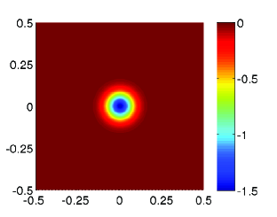
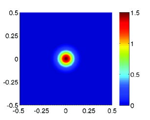
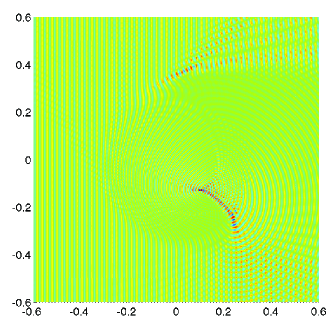
In this section, we consider problems where the scattering potential $b(\bm{x})$ is given by a Gaussian bump. Since $b$ has radial symmetry, we may compute an accurate reference scattering solution by solving a series of ODEs, as explained in Appendix A. With $\kappa=40$ (so that the square $\Omega$ is around six free-space wavelengths on a side), and $\bm{\mathsf{w}}=(1,0)$, we consider two problems given as follows,

Bump 1:	$b(\bm{x})=-1.5e^{-160|\bm{x}|^{2}}$,
Bump 2:	$b(\bm{x})=1.5e^{-160|\bm{x}|^{2}}$.

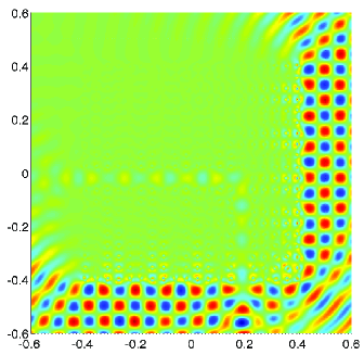
For Bump 1, the bump region has an increased refractive index, varying from 1 to around 1.58, which can be interpreted as an attractive potential. For Bump 2, the potential is repulsive, causing the waves to become slightly evanescent near the origin (here the refractive index decreases to zero then becomes purely imaginary, but note that this does not correspond to absorption.) Figure 6 illustrates the geometry and the resulting real part of the total field for each experiment.

(a)		(b)
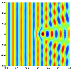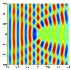(c)		(d)

Figure 6. Plots (a) and (b) illustrate $b(\bm{x})$ for experiments Bumps 1 and Bumps 2 in section 5.1. Plots (c) and (d) illustrate the real part of the total field for each experiment respectively.

Let $\tilde{u}$ denote the approximate total field constructed via the proposed method, and $u$ denote the reference total field computed as in Appendix A. Table 1 reports

$N$:	the number of discretization points used by the composite spectral method in $\Omega$,
$n$:	the number of discretization points used for discretizing the BIE,
$\operatorname{Re}\tilde{u}(0.5,0)$:	real part of the approximate solution at $(0.5,0)$ (on ${\partial\Omega}$),
$e_{1}$:	$=|u(0.5,0)-\tilde{u}(0.5,0)|$,
$\operatorname{Re}\tilde{u}(1,0.5)$:	real part of the approximate solution at $(1,0.5)$ (outside of $\Omega$),
$e_{2}$:	$=|u(1,0.5)-\tilde{u}(1,0.5)|$.

In the table, the number of levels $M$ grows from 2 to 5, roughly quadrupling $N$ each time. High-order convergence is apparent, reaching an accuracy of 9-10 digits (accuracy does not increase much beyond 10 digits). At the highest $N$, there are about 50 gridpoints per wavelength at the shortest wavelength occurring at the center of Bump 1.

	$N$	$n$	$\operatorname{Re}\tilde{u}(0.5,0)$	$e_{1}$	$\operatorname{Re}\tilde{u}(1,0.5)$	$e_{2}$
Bump 1	3721	640	-0.98792561833285	7.75e-05	-1.12207402682737	5.09e-05
	14641	800	-0.987981264965721	1.78e-07	-1.12205758254400	8.18e-08
	58081	1120	-0.987981217277174	2.56e-09	-1.12205766387011	1.15e-10
	231361	1760	-0.987981215350216	9.31e-10	-1.12205766378840	7.90e-11
Bump 2	3721	640	-0.0470314782486572	4.82e-05	-1.01063677552351	3.23e-05
	14641	800	-0.0470619180279044	4.25e-08	-1.01065022958956	7.32e-08
	58081	1120	-0.0470619010992819	1.32e-09	-1.01065028579517	1.29e-10
	231361	1760	-0.0470619007119554	5.07e-10	-1.01065028569638	4.36e-11

Table 1. Approximate solutions and pointwise errors for the experiments in section 5.1

(a)	(b)
(c)

Figure 7. Plots of the different scattering potentials $b$ inside $\Omega$ in section 5.2.

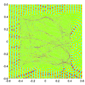
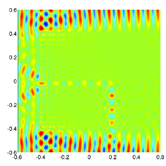
5.2. Performance for challenging scattering potentials

This section illustrates the performance of the numerical method for problems with smoothly varying wave speed inside of $\Omega$.

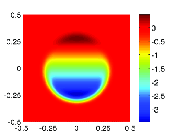
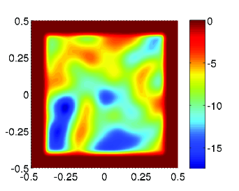
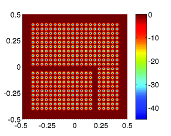
We consider three different test cases of scattering potential $b$. They are

Lens:	A vertically-graded lens (Figure 7(a)), at wavenumber $\kappa=300$.
	Specifically, $b(\bm{x})=4(x_{2}-0.2)[1-{\rm erf}(25(|\bm{x}|-0.3))]$, where $\bm{x}=(x_{1},x_{2})$.
	The maximum refractive index is around 2.1
Random bumps:	The sum of $200$ wide Gaussian bumps randomly placed in $\Omega$, rolled off to zero
	(see Figure 7(b)) giving a smooth random potential at wavenumber $\kappa=160$.
	The maximum refractive index is around 4.3.
Photonic crystal:	$20\times 20$ square array of small Gaussian bumps (with peak refractive index 6.7)
	with a “waveguide” channel removed (Figure 7(c)). The wavenumber $\kappa=77.1$
	is chosen carefully to lie in the first complete bandgap of the crystal.

For the first two cases, $\Omega$ is around 70 wavelengths on a side, measured using the typical wavelength occurring in the medium (for the lens case, it is 100 wavelengths on a side at the minimum wavelength). This is quite a high frequency for a variable-medium problem at the accuracies we achieve. In these two cases the waves mostly propagate; in contrast, in the third case the waves mostly resonate within each small bump, in such a way that large-scale propagation through the crystal is impossible (hence evanescent), except in the channel.

For each choice of varying wave speed, the incident wave is in the direction $\bm{\mathsf{w}}=(1,0)$ (we remind the reader that the method works for arbitrary incident direction). For the photonic crystal, we also consider the incident wave direction $\bm{\mathsf{w}}=(-\sqrt{2}/2,\sqrt{2}/2)$. There are no reference solutions available for these problems, hence we study convergence.

In addition to the number of discretization points $N$ and $n$, Table 2 reports

$\operatorname{Re}\tilde{u}(0.25,0)$:	real part of the approximate solution at $(0.25,0)$ (inside of $\Omega$),
$e_{1}$:	$=|\tilde{u}_{N}(0.25,0)-\tilde{u}_{4N}(0.25,0)|$, an estimate of the pointwise error,
$\operatorname{Re}\tilde{u}(1,0.5)$:	real part of the approximate solution at $(1,0.5)$ (outside of $\Omega$),
$e_{2}$:	$=|\tilde{u}_{N}(1,0.5)-\tilde{u}_{4N}(1,0.5)|$, an estimate of the pointwise error.

	$N$	$n$	$\operatorname{Re}\tilde{u}(0.5,0)$	$e_{1}$	$\operatorname{Re}\tilde{u}(1,0.5)$	$e_{2}$
Lens	58081	1120	-0.373405022283892	2.02e-01	-0.547735180732198	5.09e-01
	231361	1760	-0.221345395796661	3.53e-03	0.161212542340161	2.86e-03
	923521	3040	-0.218651605400620	1.61e-07	0.158422280450864	1.87e-07
	3690241	5600	-0.218651458554288	6.85e-10	0.158422464920298	6.99e-10
	14753281	10720	-0.218651458391577	-	0.158422464625727	-
Bumps	58081	1120	1.29105948477323	1.91	-0.612141744074168	0.44
	231361	1760	0.359271869087464	1.99e-02	-0.931198083868205	1.87e-02
	923521	3040	0.374697595070227	2.76e-06	-0.945752835546445	7.95e-07
	3690241	5600	0.374698518812982	3.06e-09	-0.945753626496863	1.58e-09
	14753281	10720	0.374698518930658	-	-0.945753627849080	-
Crystal	58081	1120	-0.406418011063883	2.03	-0.129067996215635	3.42e-01
	231361	1760	0.0424527158875615	1.53e-03	0.195870563479998	1.82e-4
	923521	3040	0.0437392735790711	7.30e-07	0.195981633749759	2.81e-07
	3690241	5600	0.0437393320806644	4.84e-10	0.195981570696692	7.56e-10
	14753281	10720	0.0437393324622741	-	0.195981570519668	-
Crystal	58081	1120	-0.0420633119821246	1.28	-1.20915538109562	1.37e-01
	231361	1760	0.0367128964251903	3.47e-03	-1.09529393341122	1.10e-3
$\bm{\mathsf{w}}=\left(-\frac{\sqrt{2}}{2},\frac{\sqrt{2}}{2}\right)$	923521	3040	0.0376839447575234	1.58e-06	-1.09445429347097	7.25e-07
	3690241	5600	0.0376833752064704	6.79e-10	-1.09445431363369	4.90e-9
	14753281	10720	0.0376833752704930	-	-1.09445430874556	-

Table 2. Convergence results for the experiments in section 5.2.

Table 2 shows that typically 9-digit accuracy is reached when $N\approx 3.7\times 10^{6}$ ($M=7$), which corresponds to 1921 Chebyshev nodes in each direction, or around 20 nodes per wavelength at the shortest wavelengths in each medium.

(a)		(b)
(c)		(d)

Figure 8. Plots of the real part of the total field for the four experiments in section 5.2 whose scattering potentials are shown in Figure 7: (a) lens, (b) random bumps, (c) and (d) photonic crystal with different incident wave directions.

5.3. Scaling of the method

Recall that in the case of multiple incident waves, the solution technique should be broken into two steps: precomputation and solve. Since a direct solver is used, the timing results are independent of the particular scattering potential.

For each choice of $N$ and $n$, Table 3 reports

$T_{\rm build}$:	Time in seconds to building the approximate ItI and DtN,
$T_{\rm solve}$:	Time in seconds to discretize and invert the BIE (35),
$T_{\rm apply}$:	Time in seconds to apply the inverse $A^{-1}$ of the discretized integral equation
$R_{\rm build}$:	Memory in MB required to store the ItI and solution operators in the hierarchical scheme,
$R_{\rm solve}$:	Memory in MB required to store the discretized inverse $A^{-1}$.

Figure 9 plots the timings against the problem size $N$. (The total precomputation time is the sum of $T_{\rm build}$ and $T_{\rm solve}$.) The results show that even at the largest $N$ tested, the precomputation time has not reached its asymptotic $O(N^{3/2})$; the large dense linear algebra has not yet started to dominate $T_{\rm build}$ (this may be due to MATLAB overheads). However, the cost for solving (35) and applying the inverse scale closer to expectations.

The memory usage scales as the expected $O(N\log N)$. We are not able to test beyond 15 million unknowns ($M=8$) since by that point the memory usage approaches 100 GB. However, note that if all that is needed is the far-field solution for arbitrary incident waves at one wavenumber, the $\bm{\mathsf{S}}^{\tau}$ and $\bm{\mathsf{Y}}^{\tau}$ solution matrices need not be stored, reducing memory significantly, and the final solution matrix only requires 2 GB. We note that, extrapolating from the convergence study, this $N$ should be sufficient for 9-digit accuracy for problems up to 200 wavelengths on a side.

$N$	$n$	$T_{\rm build}$	$T_{\rm solve}$	$T_{\rm apply}$	$R_{\rm build}$	$R_{\rm solve}$
3721	640	0.506	1.78	5.39e-04	9.71	6.25
14641	800	0.709	2.01	8.28e-04	48.07	9.77
58081	1120	2.90	3.01	1.73e-03	229.05	19.14
231361	1760	12.09	5.40	3.32e-03	1063.23	47.37
923521	3040	51.67	13.23	1.05e-02	4841.01	141.02
3690241	5600	231.18	40.79	4.03e-02	21716.21	478.52
14753281	10720	1081.09	185.54	1.13e-01	96273.17	1753.52

Table 3. $T_{\rm build}$ and $R_{\rm build}$ report the time in seconds and memory in MB, respectively, required for building the interior ItI operator and constructing the discretized integral equation (35). $T_{\rm solve}$ reports the time in seconds required to invert the discretized system, while $R_{\rm solve}$ reports the memory in MB to store the inverse. $T_{\rm apply}$ reports the time in seconds required to apply the inverse to the incident wave dependent data. This table is independent of the choice of potential or wavenumber.

(a)		(b)

Figure 9. Time in seconds for each step in the proposed method. (For the comparison power law graphs, the prefactors are $C_{1}=2\times 10^{-7}$ and $C_{2}=2\times 10^{-9}$.)

6. Concluding remarks

This paper presents a robust, high accuracy direct method for solving scattering problems involving smoothly varying media. Numerical results show that the method converges to high order, as expected, for choices of refractive index that are representative of challenging problems that occur in applications. Namely, for problems dominated either by propagation (lenses) or by resonances (a bandgap photonic crystal), with of order 100 wavelengths on a side, the method converges to around 9-digit accuracy with $3.7$ million unknowns. The method is ideal for problems where the far field scattering is desired for multiple incident waves, since each additional incident wave requires merely applying a dense matrix to its boundary data. For example, a problem involving $14$ million unknowns requires $21$ minutes of precomputation (to build the necessary operators), but each additional solve takes approximately 0.1 seconds. As discussed in section 4.2, for low frequency problems, these timings, and asymptotic behavior, could be improved by replacing the dense linear algebra by faster algorithms exploiting compressed representations. One remaining open question is the existence of a convenient second-kind formulation which involves the ItI map (and not the DtN map) of the domain $\Omega$.

Appendix A Reference solution for plane wave scattering from radial potentials

In this appendix we describe how we generate reference solutions with around 13 digits of accuracy for the scattering problem from smooth radially-symmetric potentials such as

(40) $$b(r)=\pm 1.5e^{-160r^{2}},$$

which are needed in section 5.1. Here $(r,\theta)$ are polar coordinates; in what follows $(x_{1},x_{2})\in\mathbb{R}^{2}$ indicate Cartesian coordinates. We choose a solution domain radius $R>0$ such that $b$ is numerically negligible outside the ball $r<R$. A plane wave incident in the positive $x_{1}$-direction is decomposed into a polar Fourier (“angular momentum”) basis via the Jacobi–Anger expansion [28, 10.12.5],

$$e^{i\kappa x_{1}}=J_{0}(\kappa r)+2\sum_{l=1}^{\infty}i^{l}J_{l}(\kappa r)\cos l\theta~{}.$$

We write $J_{l}(z)=(H^{(1)}_{l}(z)+H^{(2)}_{l}(z))/2$, and then notice that the effect of the potential $b$ on this field is to modify only the outgoing scattering coefficients. Thus, restricting to a maximum order $L$, the full field becomes

(41) $$u(r,\theta)\approx\mbox{\small$\frac{1}{2}$}[H^{(1)}_{0}(\kappa r)+a_{0}H^{(2)}_{0}(\kappa r)]+\sum_{l=1}^{L}i^{l}[H^{(1)}_{l}(\kappa r)+a_{l}H^{(2)}_{l}(\kappa r)]\cos l\theta,\qquad r>R~{}.$$

The coefficients $\{a_{l}\}$ are known as scattering phases; by flux conservation they lie on the unit circle if $b(r)$ is a real-valued function. Convergence with respect to $L$ is exponential, once $L$ exceeds $\kappa R$. For the case of (40) we choose $R=0.5$ and $L=30$.

The phases are found in the following way. For each $l=0,\dots L$ we solve the homogeneous radial ODE,

$$u_{l}^{\prime\prime}+\frac{1}{r}u_{l}^{\prime}+\left[-\frac{l^{2}}{r^{2}}+\left(1-b(r)\right)\kappa^{2}\right]u_{l}=0,\qquad 0<r<R$$

with initial conditions that correspond to a regular solution of the form $u_{l}(r)\sim cr^{l}$ as $r\to 0^{+}$ (we implement the initial condition by restricting the domain to $[r_{0},R]$ for some small number $r_{0}>0$ chosen such that the solution growing with increasing $r$ dominates sufficiently over the decaying one). For the numerical solution we use MATLAB’s ode45 with machine precision requested for absolute and relative tolerances. (We note that the standard transformation $u(r)=r^{l}U(r)$ which mollifies the behavior at $r=0$ resulted in no improvement in accuracy.) After extracting each interior solution’s Robin constant $\beta_{l}:=u^{\prime}_{l}(R)/u_{l}(R)$, and matching value and derivative to (41) at $r=R$, we get after simplification,

$$a_{l}=-\frac{\alpha_{l}^{\ast}}{\alpha_{l}},\qquad\mbox{where }\;\alpha_{l}=\kappa{H^{(1)}_{l}}^{\prime}(\kappa R)-H^{(1)}_{l}(\kappa R)\beta_{l}~{},$$

which completes the recipe for the phases. The computation time required is a few seconds, due to the large number of steps required by ode45. A simple accuracy test is independence of the phases with respect to variation in $R$. Values of $u(r,\theta)$ for $r\geq R$ may then be found via evaluating the sum in (41), and for $r<R$ by summation of the interior solutions $\{u_{l}(r)\}$.

References

- [1] W. Ang. A beginner’s course in boundary element methods. Universal Publishers, USA, 2007.
- [2] I. M. Babuska and S. A. Sauter. Is the pollution effect of the FEM avoidable for the Helmholtz equation considering high wave numbers? SIAM J. Numer. Anal., 34(6):2392–2423, 1997.
- [3] A. Bayliss, C. I. Goldstein, and E. Turkel. The numerical solution of the Helmholtz equation for wave propagation problems in underwater acoustics. Comput. Math. Appl., 11(7–8):655––665, 1985.
- [4] A. Bayliss, C. I. Goldstein, and E. Turkel. On accuracy conditions for the numerical computation of waves. J. Comput. Phys., 59(3):396–404, 1985.
- [5] M. Bebendorf. Hierarchical matrices, volume 63 of Lecture Notes in Computational Science and Engineering. Springer-Verlag, Berlin, 2008.
- [6] S. Börm. Efficient numerical methods for non-local operators, volume 14 of EMS Tracts in Mathematics. European Mathematical Society (EMS), Zürich, 2010.
- [7] S. Britt, S. Tsynkov, and E. Turkel. Numerical simulation of time-harmonic waves in inhomogeneous media using compact high order schemes. Commun. Comput. Phys., 9(3):520–541, 2011.
- [8] Y. Chen. A fast, direct algorithm for the Lippmann-Schwinger integral equation in two dimensions. Adv. Comput. Math., 16(2-3):175–190, 2002.
- [9] Y. Chen. Total wave based fast direct solver for volume scattering problems. arxiv.org., #1302.2101, 2013.
- [10] D. Colton and R. Kress. Inverse acoustic and electromagnetic scattering theory, volume 93 of Applied Mathematical Sciences. Springer-Verlag, Berlin, second edition, 1998.
- [11] R. Duan and V. Rokhlin. High-order quadratures for the solution of scattering problems in two dimensions. J. Comput. Physics, 228(6):2152–2174, 2009.
- [12] B. Engquist and A. Majda. Absorbing boundary conditions for the numerical simulation of waves. Math. Comp., 31:629–651, 1977.
- [13] B. Engquist and L. Ying. Sweeping preconditioner for the Helmholtz equation: Moving perfectly matched layers. Multiscale Mod. Sim., 9(2):686–710, 2011.
- [14] Q. Fang, P. M. Meaney, and K. D. Paulsen. Viable three-dimensional medical microwave tomography: Theory and numerical experiments. IEEE Trans. Antennas Propag., 58(2):449––458, 2010.
- [15] L. Friedlander. Some inequalities between Dirichlet and Neumann eigenvalues. Arch. Rational Mech. Anal., 116(2):153–160, 1991.
- [16] A. Gillman and P. Martinsson. A direct solver with complexity for variable coefficient elliptic PDEs discretized via a high-order composite spectral collocation method, 2013. In review.
- [17] A. Gillman, P. Young, and P. Martinsson. A direct solver O(N) complexity for integral equations on one-dimensional domains. Front. Math. China, 7:217–247, 2012. 10.1007/s11464-012-0188-3.
- [18] W. Hackbusch. A sparse matrix arithmetic based on H-matrices; Part I: Introduction to H-matrices. Computing, 62:89–108, 1999.
- [19] S. Hao, A. H. Barnett, P. G. Martinsson, and P. Young. High-order accurate Nyström discretization of integral equations with weakly singular kernels on smooth curves in the plane, 2013. in press, Adv. Comput. Math.
- [20] E. Heikkola, T. Rossi, and J. Toivanen. Fast direct solution of the Helmholtz equation with a perfectly matched layer/an absorbing boundary condition. Int. J. Numer. Meth. Engng, 57:2007–2025, 2003.
- [21] K. Ho and L. Greengard. A fast direct solver for structured linear systems by recursive skeletonization. SIAM J. Sci. Comput., 34(5):A2507–A2532, 2012.
- [22] A. Kirsch and P. Monk. An analysis of the coupling of finite-element and Nyström methods in acoustic scattering. IMA J. Numer. Anal., 14:523–544, 1994.
- [23] D. Kopriva. A staggered-grid multidomain spectral method for the compressible Navier-Stokes equations. J. Comput. Phys, 143(1):125–158, 1998.
- [24] P. Martinsson. A fast direct solver for a class of elliptic partial differential equations. J. Sci. Comput., 38(3):316–330, 2009.
- [25] P. Martinsson. A direct solver for variable coefficient elliptic PDEs discretized via a composite spectral collocation method. J. Comput. Phys., 242:460–479, 2013.
- [26] W. McLean. Strongly elliptic systems and boundary integral equations. Cambridge University Press, Cambridge, 2000.
- [27] D. P. Nicholls and N. Nigam. Exact non-reflecting boundary conditions on general domains. J. Computat. Phys., 194(1):278–303, 2004.
- [28] F. Olver, D. Lozier, R. Boisvert, and C. Clark, editors. NIST Handbook of Mathematical Functions. Cambridge University Press, 2010. http://dlmf.nist.gov.
- [29] H. Pfeiffer, L. Kidder, M. Scheel, and S. Teukolsky. A multidomain spectral method for solving elliptic equations. Comput. Phys. Commun., 152(3):253–273, 2003.
- [30] H. E. Salzer. Lagrangian interpolation at the Chebyshev points , ; some unnoted advantages. Comput. J., 15:156–159, 1972.
- [31] P. Schmitz and L. Ying. A fast direct solver for elliptic problems on Cartesian meshes in 3D, 2011. preprint.
- [32] P. Schmitz and L. Ying. A fast direct solver for elliptic problems on general meshes in 2D. J. Comput. Phys., 231(4):1314 – 1338, 2012.
- [33] L. Trefethen. Spectral Methods in MATLAB. SIAM, Philadelphia, 2000.
- [34] E. E. Tyrtyshnikov. A brief introduction to numerical analysis. Birkhäuser Boston, 1997.
- [35] E. Wadbro and M. Berggren. High contrast microwave tomography using topology optimization techniques. J. Comput. Appl. Math., 234:1773–1780, 2010.
- [36] S. Wang, M. V. de Hoop, and J. Xia. On 3D modeling of seismic wave propagation via a structured parallel multifrontal direct Helmholtz solver. Geophysical Prospecting, 59(5):857–873, 2011.
- [37] J. Xia, S. Chandrasekaran, M. Gu, and X. Li. Superfast multifrontal method for large structured linear systems of equations. SIAM J. Matrix Anal. Appl., 31(3):1382–1411, 2009.
- [38] J. Xia, S. Chandrasekaran, M. Gu, and X. S. Li. Fast algorithms for hierarchically semiseparable matrices. Numer. Linear Algebra Appl., 17(6):953–976, 2010.
- [39] B. Yang and J. Hesthaven. Multidomain pseudospectral computation of Maxwell’s equations in 3-D general curvilinear coordinates. Appl. Numer. Math., 33(1–4):281 – 289, 2000.