Low Rank Approximation Method for Efficient Green’s Function Calculation of Dissipative Quantum Transport

Abstract

In this work, the low rank approximation concept is extended to the non-equilibrium Green’s function (NEGF) method to achieve a very efficient approximated algorithm for coherent and incoherent electron transport. This new method is applied to inelastic transport in various semiconductor nanodevices. Detailed benchmarks with exact NEGF solutions show 1) a very good agreement between approximated and exact NEGF results, 2) a significant reduction of the required memory, and 3) a large reduction of the computational time (a factor of speed up as high as $150$ times is observed). A non-recursive solution of the inelastic NEGF transport equations of a $1000\leavevmode\nobreak\ \mathrm{nm}$ long resistor on standard hardware illustrates nicely the capability of this new method.

LABEL:FirstPage1 LABEL:LastPage#12

I Introduction

Modern semiconductor devices have reached such small dimensions that carrier confinement, interference effects and tunneling play an equally important role as incoherent scattering, momentum and energy relaxation do. Moore (1995); Yang et al. (2004); Yu et al. (2002); Huang et al. (1999) The non-equilibrium Green’s function (NEGF) method is among the most widely employed methods to describe carrier dynamics in open quantum systems. Kadanoff and Baym (1962); Keldysh (1965) In fact, the NEGF method is applied to a constantly growing variety of systems ranging from phonon transport, Xu et al. (2008); Mingo (2006) spin transport, Yamamoto et al. (2005); Sergueev et al. (2002) electron dynamics in metals, Chen et al. (2005); Ke et al. (2008); Belzig et al. (1999) organic moleculesFrederiksen et al. (2007) and fullerenes, Sato et al. (2008); Damle et al. (2002); Li and Zhang (2008); Schull et al. (2009) and semiconductor nano-structures. Zheng et al. (2006); Havu et al. (2004); Lazzeri et al. (2005); Luisier et al. (2006); Do et al. (2006) Unfortunately, the basic NEGF equations are numerically cumbersome and extremely time demanding to solve. Therefore, several different approximations for particular devices and situations have been developed to reduce the numerical costs. The recursive Green’s function method reduces the peak numerical burden to a device dependent sub-block matrix of the system’s hamiltonian, and the computational cost scales linearly with the number of blocks but cubically with the block size. Lake et al. (1997); Ferry and Goodnick (1997) It is widely used for the simulations with one transport direction such as FinFETs Yang et al. (2004); Yu et al. (2002); Huang et al. (1999) and nanowire structure. Wang et al. (2004) Mode space approaches in similar wire structures as well as the newly developed Equivalent transport mode method separate the transport direction from transverse confinement directions thus reducing the block size in each layer. Polizzi and Ben Abdallah (2002); Wang et al. (2004); Mil’nikov et al. (2012) All these methods usually require a clear distinction between the transport direction and transverse degrees of freedom. When this distinction gets blurred, as in the case of incoherent scattering, their numerical efficiency drops significantly. A very efficient method to solve ballistic NEGF equations is the contact block reduction method (CBR). Mamaluy et al. (2003); Birner et al. (2009); Mamaluy et al. (2005) However, this method does not offer self-consistent incoherent scattering capability. Niche applications of the NEGF method have used sophisticated Wannier and Wannier Stark functions to represent the transport problem in the presence of many incoherent scattering mechanisms. Lee et al. (2006); Wacker (2008) This specific basis representation, however, is custom made for quantum cascade lasers and superlattices.

In this work, the low rank approximation (LRA) method is adapted to the NEGF equations of electrons in simiconductors in the presence of inelastic scattering on phonons. Markovsky (2012) This method is an extension of the ”basis reduction method” of Greck et al. Greck (2008, ) The concept of low rank approximation is inherited from data modeling in control theory Song et al. (2008), machine learning Markovsky (2012), signal processing Kirsteins and Tufts (1994), bioinformatics Fu and Albus (1977) for microarray data analysis etc. In the framework of NEGF, the transport problem is transformed from the original basis representation, i.e. in this work real space in effective mass hamiltonian presentation, to a more appropriate basis of quasi-particle states that are close to the quasi-particles of the actual device. In this representation, the number of required basis functions is much less than in the original space, which allows to reduce the numerical costs significantly. In so far, this method is closely related to the beforementioned mode space approach. However, the LRA method is a generalization to that, since it does not have any prerequisites to the device geometry. In addition, the LRA implementation of this work uses a third basis representation to enable real space defined inelastic scattering mechanisms.

In Sec. II, the method of this work is introduced, its numerical complexity is analyzed and differences of this method with existing approximations are discussed. In Sec. III, transport in homogeneous resistor and a resonant tunneling diode is calculated. The comparisons of exact NEGF calculations with the LRA approximated results show the accuracy of the presented method. Limitations that this method (as every approximation approach does) faces are also discussed in this section. To exemplify the computational strength of the LRA method, electronic transport in a $1000\leavevmode\nobreak\ \mathrm{nm}$ resistor is calculated in the end of this section. Energy resolved density spectrum illustrates the transition from ballistic to drift diffusion transport in this resistor. The paper concludes with a summary in Sec. IV.

II Method

II.1 Low Rank Approximation Method

NEGF calculations are time consuming since they involve the inversion and multiplication of matrices with the rank $N$ of the system’s hamiltonian. The fundamental concept of the LRA method is to reduce the computational cost by transforming the NEGF equations into a space of lower rank $n$ and solving the equations therein. It is expected that the closer the basis functions of the lower rank space are to the physically relevant quasi-particles of the device, the better the LRA approximation is and the smaller the ratio $n/N$ can be chosen. The solution of the NEGF equations and all observables can be transformed back into the original space after self-consistent calculation is achieved. In this way, the matrices that represent the Green’s functions and self-energies still have the lower rank $n$, but the dimensionality $N$ which is required to maintain compatibility with other equations (such as the Poisson equation) that might still be given in the original space.

This method is exemplified on the stationary vertical transport in laterally homogeneous quantum well hetero-structures that are in contact with two charge reservoirs. The electron structure is represented in terms of a single band effective mass hamiltonian $H_{0}$ that is represented in a basis of $N$ position eigenfunctions

$$H_{0}=\frac{-\hbar^{2}}{2}\frac{\mathrm{d}}{\mathrm{d}z}\frac{1}{m^{\ast}\left(z\right)}\frac{\mathrm{d}}{\mathrm{d}z}+\frac{\hbar^{2}k_{\parallel}^{2}}{2m^{\ast}\left(z\right)}+V\left(z\right),$$ (1)

where $k_{\parallel}$ is the in-plane electron momentum and $V\left(z\right)$ represents a position dependent potential. In the NEGF formalism, stationary transport is determined by four coupled partial differential equations

$$G^{R} =\left(E-H_{0}-\Sigma^{R}\right)^{-1},$$

$$G^{<} =G^{R}\Sigma^{<}G^{R{\dagger}},$$

$$\Sigma^{<} =G^{<}D^{<},$$

$$\Sigma^{R} =G^{R}D^{R}+G^{R}D^{<}+G^{<}D^{R}.$$ (2)

Here, the electronic retarded and lesser Green’s functions are given by $G^{R}$, $G^{<}$, respectively. Kubis et al. (2009); Datta (2005, 1997) $D$ is the sum of all environmental Green’s functions that incorporate e.g. phonons, and $\Sigma$ denotes the self-energies. The devices are in contact with two charge reservoirs, represented with contact self-energies. Datta (2005, 1997) If not explicitly stated otherwise, all calculations in this work include inelastic scattering by longitudinal acoustic phonons given by the scattering self-energiesKubis et al. (2009); Mátyás et al. (2010); Kubis et al. (2008)

$$\Sigma_{\text{ac}}^{<,R}\left(z,z^{\prime},k_{\parallel},E\right)=\frac{1}{\left(2\pi\right)^{3}}\frac{k_{B}TD^{2}_{ac}}{2\rho v_{s}^{2}}$$

$$\times\int\mathrm{d}\vec{q}_{\parallel}\mathrm{d}q_{z}\mathrm{e}^{iq_{z}\left|z-z^{\prime}\right|}\left[\tilde{G}^{<,R}\left(z,z^{\prime},\left|\vec{k}_{\parallel}-\vec{q}_{\parallel}\right|,E+\hbar\omega_{q}\right)\right.$$

$$\left.+\tilde{G}^{<,R}\left(z,z^{\prime},\left|\vec{k}_{\parallel}-\vec{q}_{\parallel}\right|,E-\hbar\omega_{q}\right)\right],$$ (3)

with the energy-averaged Green’s functions

$$\tilde{G}\left(z,z^{\prime},q_{\parallel},E\right)=\frac{1}{2\hbar\omega_{D_{ac}}}\int_{E-\hbar\omega_{D_{ac}}}^{E+\hbar\omega_{D_{ac}}}\mathrm{d}E^{\prime}G\left(z,z^{\prime},q_{\parallel},E^{\prime}\right).$$ (4)

The acoustic deformation potential and the material density is denoted by $D_{ac}$ and $\rho$, respectively. The acoustic phonon frequency is $\omega_{q}$ and $v_{s}$ is the sound velocity. Kubis et al. (2009); Mátyás et al. (2010); Kubis et al. (2008) The Debye frequency $\omega_{D_{ac}}$ limits the width of the average.

As the first step of this method, the $n$ eigenfunctions of the free particle Hamiltonian $H_{0}$ with Neumann boundary conditions are solved that have smallest eigen energy $E_{i}$

$$H_{0}\phi_{i}=E_{i}\phi_{i},\text{ }i=1,2,\ldots n.$$ (5)

Hereby, $n$ is chosen such that the energy $E_{n}$ is about several $k_{B}T$ above the highest chemical potential of all leads (with the Boltzmann constant $k_{B}$ and the temperature $T$). Thereby, all quasi-particles with energies below $E_{n}$ are appropriately considered in the calculation. This is essential to capture all occupied electronic states and to predict the density accurately. It is worth to mention that if only the transmission around a given energy $E_{0}$ is required, it is sufficient to consider eigenstates of a few $k_{B}T$ around $E_{0}$.

In the second step, the $n$ orthonormal eigenstates $\phi_{i}$ are set into the $n$ columns of a $N\times n$ dimensional matrix $S$. This matrix $S$ is unitary in the $n$ dimensional space $\Omega$ spanned by the wavefunctions $\phi_{i}$, but note that it is not unitary in the $N$ dimensional real space of step one

$$S^{\dagger}S=I,$$ (6)

$$SS^{\dagger}\neq I.$$ (7)

To define the locality/non-locality of scattering self-energies, the position operator of the real space discretization $X$ is transformed into the reduced rank basis in the third step

$$X_{S}=S^{{\dagger}}XS.$$ (8)

The position operator $X$ is a diagonal matrix, whereas the reduced rank matrix $X_{S}$ is a dense matrix. Therefore, the operator $X_{S}$ is diagonalized to find the reduced rank position eigenfunction basis $\left\{\psi_{i}\right\}$

$$X_{S}\psi_{i}=x_{i}\psi_{i},\text{ }i=1,2,\ldots n.$$ (9)

These orthonormal basis functions $\left\{\psi_{i}\right\}$ define the columns of a squared, unitary $n\times n$ transformation matrix $P$. In the basis $\left\{\psi_{i}\right\}$ the NEGF equations Eqs. (2) read

$$G_{P}^{R} =\left(P^{{\dagger}}T^{{\dagger}}\left(E-H_{0}\right)TP-\Sigma_{P}^{R}\right)^{-1},$$

$$G_{P}^{<} =G_{P}^{R}\Sigma_{P}^{<}G_{P}^{R{\dagger}},$$

$$\Sigma_{P}^{<} =G_{P}^{<}D_{P}^{<},$$

$$\Sigma_{P}^{R} =G_{P}^{R}D_{P}^{R}+G_{P}^{R}D_{P}^{<}+G_{P}^{<}D_{P}^{R}.$$ (10)

Since every basis function $\psi_{i}$ is associated with a position $x_{i}$ the equations above are discretized in a reduced rank real space representation. Position dependent scattering self-energies such as the acoustic phonon scattering self-energy in Eq. (3) are then self-consistently solved with the non-equilibrium Green’s functions in the numerically efficient reduced rank real space. The introduction of the reduced real space helps to avoid the back-transformation of the Green’s functions into the original real space in the self-consistent calculation when position dependent scattering self-energy is calculated.

Once the NEGF equations Eqs. (10) are converged, the diagonal and the first off-diagonal elements of $G^{<}$ are transformed back into the original rank $N$ real space representation. Observables such as the density or the current density can then be evaluated in the original, high resolution real space. However, the rank of the Green’s functions in the $N$ dimensional system equals the dimension of the space they are solved in, i.e. the rank equals $n$. The smaller $n$ is compared to $N$, the more unreliable the $N$ dimensional spatial information is, i.e. the stronger deviations of the LRA results from the exact results are. It will be shown as one of the example results in the next section, that the LRA approximated current density oscillates in the original space, although the physical current of exact calculations is conserved. To predict current voltage characteristics in the LRA method, this inhomogenous current density is averaged over the device excluding areas within $\Delta N/n$ from the leads (where $\Delta$ is the average mesh point distance in the original real space representation).

II.2 Comparison with existing efficient NEGF algorithms

It is important to highlight some differences of this method with other, well established efficient NEGF algorithms such as the CBR method Mamaluy et al. (2003); Birner et al. (2009); Mamaluy et al. (2005), mode space approaches Polizzi and Ben Abdallah (2002); Wang et al. (2004) and recursive Green’s function method. Lake et al. (1997); Ferry and Goodnick (1997)

In the CBR method, the NEGF equations are first transformed into an efficient representation to utilize the fact that ballistic calculations require only some sections of the retarded Green’s function $G^{R}$ to be solved. A rectangular transformation that reduces the rank of the NEGF equations is applied only after that first transformation. Although the CBR method is very efficient, it is fundamentally limited to ballistic calculations.

The mode space approach assumes a separation Ansatz for the wave functions of propagating quasi-particles. Typically, the Ansatz requires confined modes or plane waves perpendicular to the transport direction. The mode space approach allows a significant rank reduction of the NEGF equations. The computational burden is even further reduced if these modes are well separated in energy and the particle propagation does not couple different modes. However, if the device contains inhomogeneities (impurities, non conformal confinement, etc.) the number of the modes is no longer a conserved quantum number. Then, the modes are coupled and the rank of the mode space has to be large to predict transport without loss of accuracy.

The recursive Green’s function method allows to limit the calculation of the retarded Green’s function to selected parameter intervals of the propagation space (i.e. sub-matrices of $G^{R}$, when $G^{R}$ is represented in matrix form). This allows limiting ballistic NEGF calculations on the required elements of $G^{R}$ only, which results in much faster transport solutions than the case when the complete $G^{R}$ is solved. Lake et al. (1997) NEGF that includes incoherent scattering, however, requires the full $G^{R}$ which deteriorates the advantages of this recursive method.

In contrast to these three methods, the LRA method allows the inclusion of any incoherent scattering as well as arbitrary device geometries. The ”modes/sub-block matrix” of the LRA method are device dependent wave functions that automatically include non-conformal confinement - if such confinement appears.

II.3 Numerical Complexity and Memory Usage Analysis

Coherent quantum transport calculations for realistically extended devices have been shown to efficiently consume the computational power of over 220,000 processing cores. Klimeck and Luisier (2010); Haley et al. (2009) Incoherent NEGF based calculations require about 100x more computational power, are limited to generally unrealistical small structures, and can only scale to about 100,000 cores. Luisier and Klimeck (2009); Luisier (2010) Involving incoherent scattering in realistically extended devices requires dramatically large computational resources.

The numerical complexity and memory usage of self-consistent NEGF calculations reduce when the LRA method is applied. To qualify that, this section compares the number of floating point operations and the memory usage of a ”conventional” NEGF calculation with an approximated ballistic NEGF solution that employs the LRA method. In the following, the transport problem is assumed to be originally discretized with $N$ orthogonal basis functions. Within the LRA method, the rank of the NEGF equations is reduced down to $n$. The energy and other conserved quantum numbers of the NEGF equations are resolved with a mesh of $N_{E}$ points. To get a conserved current density within the self-consistent Born approximation, $N_{i}$ iterations of the Green’s functions and self-energies are required. The integral in Eq. (3) is solved with $N_{ph}$ energy points.

Exact NEGF

The exact solution of one retarded Green’s function involves the inversion of a $N$ dimensional matrix which requires $O\left(N^{3}\right)$ floating point operations. The solution of each lesser Green’s function involves two matrix-matrix products with a numerical load of $O\left(N^{3}\right)$ floating point operations. The solution of the local scattering self-energy of Eq. (3) is $O\left(N_{ph}\times N\right)$ for each energy point in each iteration. In total, solving the NEGF equations exactly requires $N_{E}\times N_{i}\times\left(O\left(N^{3}\right)+O\left(N_{ph}\times N\right)\right)$ floating point operations, while the memory needed to store the matrix representation of Green’s functions and self-energies is $N_{E}\times O\left(N^{2}\right)$ floating point numbers.

Approximate NEGF

The LRA method can be decomposed into three steps: 1) the transformation of the NEGF equations into the reduced space, 2) the solution of the NEGF equations within the reduced space and 3) the back-transformation of some relevant results into the original space. Step 1) requires first to get the eigen states that construct the transformation matrix, i.e. $O\left(N^{2}n\right)$ floating point operations. The memory used to store the transformation matrix is $O\left(Nn\right)$ floating point numbers. The transformation of the device’s hamiltonian into the reduced space requires then $O\left(N^{2}n\right)$ floating point operations. The contact self-energies have to be transformed for every energy point in every iteration. Since the contact self-energy is zero except for the mesh points adjacent to the leads in the original space, each transformation requires only $N_{E}\times N_{i}\times O\left(n^{2}\right)$ floating point operations and $N_{E}\times O\left(n^{2}\right)$ floating point numbers to be stored. Solving the NEGF equations in the reduced space in step 2) requires $N_{E}\times N_{i}\times O\left(n^{3}\right)$ floating point operations and memory usage of $N_{E}\times O\left(n^{2}\right)$ floating point numbers. The calculation of the acoustic phonon self-energy costs $O\left(N_{ph}\times n\right)$ operations in the reduce real space for each energy point in each iteration. To calculate the energy resolved densities and current densities Kubis et al. (2009); Mátyás et al. (2010); Kubis and Vogl (2011) in the original space, the step 3) requires to back-transform the diagonal and the two first off-diagonals of $G^{<}$ of the original space. This transformation requires $N_{E}\times O\left(Nn^{2}\right)$ floating point operations and memory usage of $N_{E}\times O\left(N\right)$ floating point numbers.

In a typical effective mass NEGF calculation, the simulation setup reads $N=100$, $n=10$, $N_{E}=1000$, $N_{i}=10$ and $N_{ph}=10$. According to the analysis above, the numerical complexity of standard NEGF calculation in the typical effective mass situation is $O\left(10^{10}\right)$ floating point operations, and the memory usage is $O\left(10^{7}\right)$ floating point numbers; the numerical complexity of LRA approximated NEGF calculation is $O\left(10^{7}\right)$ floating point operations, and the memory usage is $O\left(10^{5}\right)$ floating point numbers. This observation demonstrates clearly that LRA method can reduce both numerical cost and memory usage significantly.

The comparison of the amount of floating point operations and memory usage between the exact and the approximated LRA approach illustrate that the LRA method offers approximated solutions of the NEGF equations much faster and with a much smaller memory load than the exact solutions. In fact, one can easily find NEGF equations of state of the art devices that are only solvable when the LRA method is applied. To illustrate this, section III.3 shows LRA approximated NEGF results of a $1000\leavevmode\nobreak\ \mathrm{nm}$ homogeneous resistor with inelastic acoustic phonon scattering calculated on single CPU.

III Results and Discussions

All devices in this section are laterally homogeneous layers grown in the $z$-direction. Stationary transport along the $z$ direction is calculated for conduction band electrons in the effective mass approximation. In the original real space discretization (i.e. before LRA transformations are applied), the Green’s functions and self-energies are functions of two propagation coordinates $z$ and $z^{\prime}$, the absolute in-plane momentum $k_{\parallel}$ and the electron energy $E$. All devices of a given length $L$ are considered to be in contact with two charge reservoirs at $z=0$ and $z=L$, respectively.

III.1 Homogeneous structure

Conduction band electrons of a $50\leavevmode\nobreak\ \mathrm{nm}$ thick, homogeneous layer of GaAs with an effective mass of $m^{\ast}=0.067\leavevmode\nobreak\ m_{0}$ Landolt-Börnstein and Madelung (1987) are considered in this section. The NEGF equations are discretized with a $0.5\leavevmode\nobreak\ \mathrm{nm}$ mesh spacing. The Fermi energies in both leads are assumed to agree with the respective conduction band edge. The temperature is set to $300\leavevmode\nobreak\ \mathrm{K}$. The conduction band in the device is set to be constant in the first and last $5\leavevmode\nobreak\ \mathrm{nm}$ of the device and to drop linearly by the amount of the applied bias voltage in the central $40\leavevmode\nobreak\ \mathrm{nm}$ of the device.

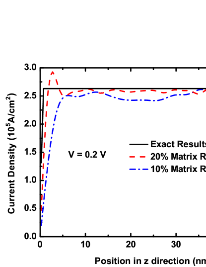
Figure 1 shows the spatially resolved current density that results from an exact NEGF calculation as well as current densities of LRA calculations when the matrix rank is reduced to $20\%$ and $10\%$ of the original space. The exact calculation yields a spatially constant current in the device, since inelastic phonon scattering is included through a converged self-consistent Born approximation. At the device boundaries the matrix elements of the exact contact self-energy is non-zero as is common in the NEGF method. This non-vanishing self-energy allows electrons to enter and leave the device, thus this contact self-energy violates current conservation at the device boundaries. In the LRA method, the contact self-energies are transformed into dense matrices. Their largest elements are still located close to the device boundaries, which causes the largest current fluctuations there. The larger the matrix rank reduction is, the larger contact self-energy matrix elements within the device are. Consequently, the larger the rank reduction is, the maximum amplitude of current density fluctuations within the device is the higher. The smaller the rank of the reduced real space is, the more dense the contact self-energies are. This allows electrons to leave/enter the device at/to any device point in the reduced rank space. The non-constant current densities in Fig. 1 in the original real space indicate this kind of violation of particle conservation.

Figure 1: Spatially resolved current density in the homogeneous structure described in the main text Sec. III.1 with a linear potential drop of $0.2\leavevmode\nobreak\ \mathrm{eV}$. The lines show result calculated with the NEGF method solved exactly (solid) and with the NEGF method solved approximately with a reduction of the matrix rank down to 20% (dashed) and 10% (dash-dotted).

Similar to the current fluctuations the density deviates from the exact solution stronger, if the rank of the NEGF equations is reduced more: Figure 2 shows the electron density in the homogenous layer of GaAs in equilibrium and at finite applied bias voltage. In both cases, the deviations are strongest close to the leads.

Figure 2: Calculated electron density of the homogeneous device of Fig. 1 in equilibrium (a) and when a linear potential drop of $0.2\leavevmode\nobreak\ \mathrm{eV}$ is assumed (b). Results of an exact NEGF calculation (solid) are compared with approximated NEGF calculations where the NEGF equations’ matrix rank is reduced down to 20% (dased) and 10% (dash-dotted).

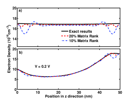
Both of the above figures indicate that the LRA method can reproduce exact NEGF results in the device center up to close to the leads. This motivated the device average of the current density described in Sec. II.1. All remaining current densities in this paper are such device averaged results.

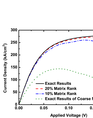
Figure 3 shows I-V characteristics of the $50\leavevmode\nobreak\ \mathrm{nm}$ thick homogeneous GaAs layer that have been calculated in the exact NEGF method, as well as in the approximate LRA method with various rank reduction levels. In addition, Fig. 3 also shows an exact NEGF calculation of the same device with a ten times coarser grid mesh. Similar to previous figures, the deviation of the LRA approximated from the exact NEGF results is larger, the larger the rank reduction is. Nevertheless, a reduction of rank to $10\%$ is still able to well reproduce the I-V characteristics, since only a small fraction of electronic states in the low energy range contributes to the current density. In contrast, results of exact NEGF calculations with a ten times coarser grid deviate significantly from the full rank result: Such a coarser real space mesh yields a different effective electron dispersion Datta (2005, 1997) that deviates from the parabolic dispersion within the relevant energies.

It is worth to mention that the boundary conditions for the electronic wave functions of Eq. (5) are relevant for the efficiency of the LRA method. In agreement to similar findings of Mamaluy et al., Mamaluy et al. (2003); Birner et al. (2009); Mamaluy et al. (2005) basis functions with Dirichlet boundary conditions turned out to be inferior to Neumann conditions.

Figure 3: Comparison of I-V characteristic of the structure of Fig. 1 determined in exact NEGF calculations (solid) and in approximated NEGF solutions where the NEGF matrix rank is reduced to 20% (dashed) and 10% (dash-dotted). Also shown are the results for an exact NEGF calculation of the same device when it is discretized with a 10 times coarser real space mesh (dotted).

The LRA method and standard NEGF calculations were implemented in Matlab with 8 cores parallelization. For this concrete homogeneous structure calculation, the measured computational time for matrix rank reductions down to $10\%$ and $20\%$ is reduced by factories of $35\mathrm{X}$ and $87\mathrm{X}$ respectively compared to the full solutions, as listed in Table 1. In our non-optimized LRA Matlab implementation, most of the time is spent to transform Green’s functions between different basis representations. If further optimization on matrix transformation is performed (as discussed in Sec.II.3), the factor of speed up can be even larger.

	$\mathbf{10\%}$ Matrix Rank	$\mathbf{20\%}$ Matrix Rank	Exact Solution
$\mathbf{50\leavevmode\nobreak\ \textbf{nm}}$ resistor	$42\mathrm{s}/87\mathrm{X}$	$104\mathrm{s}/35\mathrm{X}$	$3658\mathrm{s}/1\mathrm{X}$
RTD structure	$287\mathrm{s}/150\mathrm{X}$	$1107\mathrm{s}/39\mathrm{X}$	$43058\mathrm{s}/1\mathrm{X}$
$\mathbf{1000\leavevmode\nobreak\ \textbf{nm}}$ resistor	too aggressive reduction	$459\mathrm{hr}$	memory exceed

Table 1: The measured time consumptions for the three examples in Sec. III for matrix rank reductions down to $10\%$ and $20\%$ as well as exact NEGF solutions are listed. The LRA method and standard NEGF calculations were implemented in Matlab with 8 cores parallelization.

III.2 Resonant tunneling diode

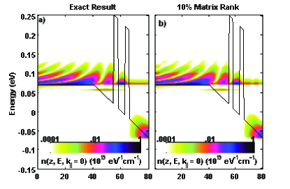
This section explores the compatibility of the LRA method in quantum confined systems. The NEGF equations are solved in a $80\leavevmode\nobreak\ \mathrm{nm}$ GaAs/Al_0.3Ga_0.7As resonant tunneling diode (RTD) structure at $100\leavevmode\nobreak\ \mathrm{K}$. The RTD consists of two $3\leavevmode\nobreak\ \mathrm{nm}$ wide Al_0.3Ga_0.7As barriers and a $5\leavevmode\nobreak\ \mathrm{nm}$ quantum well in the center. In addition, a $40\leavevmode\nobreak\ \mathrm{nm}$ flat band region is located at emitter region. The effective mass for GaAs is $0.067\leavevmode\nobreak\ m_{0}$ and $0.0919\leavevmode\nobreak\ m_{0}$ for Al_0.3Ga_0.7As. Kubis et al. (2009); Mátyás et al. (2010); Kubis and Vogl (2007); Landolt-Börnstein and Madelung (1987) The band offset between these two materials is $230\leavevmode\nobreak\ \mathrm{meV}$. Kubis et al. (2009); Mátyás et al. (2010); Kubis and Vogl (2007); Landolt-Börnstein and Madelung (1987) In the original real space representation, the device is discretized with a grid spacing of $0.5\leavevmode\nobreak\ \mathrm{nm}$. The Fermi energies in the leads are set $0.005\leavevmode\nobreak\ \mathrm{meV}$ beneath the respective conduction band edges. The potential profile is assumed to be constant in the left most $40\leavevmode\nobreak\ \mathrm{nm}$ and to drop linearly in the remaining RTD region. This is illustrated by the solid line in Fig. 4 (a) and (b) which show the same assumed conduction band profile of the RTD in an exact NEGF calculation (a) and a $10\%$ LRA approximated NEGF calculation (b). Figures 4 (a) and (b) also show contour graphs of the energy and spatially resolved electron density of the RTD at vanishing in-plane momentum ($k_{\parallel}=0$)Lee et al. (2006); Lee and Wacker (2003); Wacker (2008); Kubis et al. (2009); Mátyás et al. (2010) when a voltage of $0.1375\leavevmode\nobreak\ \mathrm{V}$ is applied. Both results agree very well: Fig. 4 (b) deviates from (a) only at the energy of about $0.07\leavevmode\nobreak\ \mathrm{eV}$ and positions $z\in\left[65,80\right]$. Even the confined state in the triangular quantum well locating at left of the first RTD barrier (at energy of about $0.05\leavevmode\nobreak\ \mathrm{eV}$ and position $50\leavevmode\nobreak\ \mathrm{nm}$) is well reproduced in the LRA calculation. This is remarkable, since electrons can enter this state effectively only via inelastic scattering. Therefore, inelastic scattering and tunneling are well reproduced with the LRA method.

Figure 4: Conduction band profile (solid line) and contour plot of the energy resolved electron density of the RTD structure described in the main text Sec. III.2. The energy resolved density is calculated within the NEGF method exactly (a) and approximately by a reduction of the NEGF equations’ matrix rank to 10% (b). The filling of bound state in triangular well by inelastic acoustic phonon scattering is well captured in the approximate method.

That can also be seen in Fig. 5, which shows the I-V characteristics of this RTD structure calculated in the exact NEGF method, as well as in the LRA method with $10\%$ and $3.1\%$ of the original matrix rank. Neither the current amplitude nor the resonance value get significantly altered when the NEGF equations are solved with only $10\%\,$ of the original matrix rank. If the matrix rank is reduced too much, electronic states that are relevant for the transport are neglected. Consequently, the current density starts to deviate then. This is illustrated in Fig. 5 with the I-V characteristic results of a LRA approximated NEGF calculation of only $3.1\%$ of the original matrix rank. As stated in Sec. II.1, the ratio of the matrix rank reduction can be estimated from the energy interval in which the states are occupied.

Figure 5: I-V characteristic of the RTD structure of Fig. 4 calculated exactly (solid line) and approximately with 10% (dashed) and 3.1% (dash-dotted) of the original NEGF equations’ matrix rank.

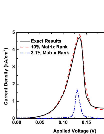
For this RTD example, the measured computational time for matrix rank reductions down to $10\%$ and $20\%$ is reduced by factories of $39\mathrm{X}$ and $150\mathrm{X}$ respectively compared to the full solutions, as listed in Table 1.

III.3 1000nm long GaAs resistor

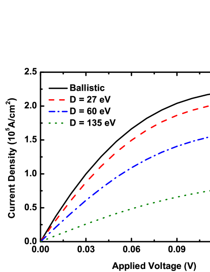
The new LRA method is not only more efficient than the standard NEGF approach, it also opens up a space of device configurations that previously could not be tackled. This section considers electronic transport in the presence of inelastic phonon scattering in a $1000\leavevmode\nobreak\ \mathrm{nm}$ long homogeneous GaAs layer. In the range of $100\leavevmode\nobreak\ \mathrm{nm}$ within the source and the drain contact/device interface, the conduction band is assumed to be constant. In the remaining device, the conduction band drops linearly according to the applied bias voltage. The temperature of the phonon bath and the electrons in the leads is $300\leavevmode\nobreak\ \mathrm{K}$ and the Fermi levels of the leads are set $0.1\leavevmode\nobreak\ \mathrm{eV}$ above the respective conduction band edge. The system is originally discretized with a mesh spacing of $1\leavevmode\nobreak\ \mathrm{nm}$. The resulting NEGF equations are approximated with a $20\%$ matrix rank. This reduces the numerical complexity of the NEGF equations such that they have been solved on a single CPU without recursive approaches. The nature of the transport is tuned from purely ballistic to almost drift diffusion like by increasing the deformation potential $D$ of the phonon scattering self-energy of Eq. (3). Hereby, three different scattering potentials have been considered: $27\leavevmode\nobreak\ \mathrm{eV}$, $60\leavevmode\nobreak\ \mathrm{eV}$ and $135\leavevmode\nobreak\ \mathrm{eV}$, which corresponds to a scattering rate of $1\times 10^{12}\leavevmode\nobreak\ \mathrm{s}^{-1}$, $5\times 10^{12}\leavevmode\nobreak\ \mathrm{s}^{-1}$ and $2.5\times 10^{13}\leavevmode\nobreak\ \mathrm{s}^{-1}$ for electrons with kinetic energy of $0.3\leavevmode\nobreak\ \mathrm{eV}$. The impact of the scattering is illustrated in Fig. 6 as it shows the calculated I-V characteristics of the device with various scattering strengths. The I-V characteristic is almost ohmic in the case of a deformation potential of $135\leavevmode\nobreak\ \mathrm{eV}$.

Figure 6: The I-V characteristic of the $1000$ $\mathrm{nm}$ homogenous structure described in the main text Sec. III.3 when different values for the deformation potential are used: $27\leavevmode\nobreak\ \mathrm{eV}$ (dashed), $60\leavevmode\nobreak\ \mathrm{eV}$ (dash-dotted) and $135\leavevmode\nobreak\ \mathrm{eV}$ (dotted), and the ballistic results are shown as a solid curve. All results are determined from approximated NEGF equations with a matrix rank of 20% of the original rank.

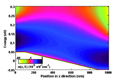
The nature of transport at this large deformation potential can be understood from Fig. 7. It shows the energy and spatially resolved electron density for the $1000\leavevmode\nobreak\ \mathrm{nm}$ long resistor in the case of $0.1\leavevmode\nobreak\ \mathrm{V}$ applied bias voltage. Electrons that originate from the source contact propagate about $400\leavevmode\nobreak\ \mathrm{nm}$ in the device before they start to significantly dissipate energy. Then, however, these electrons follow the potential drop of the device and thereby start to maintain a local equilibrium distribution. In this way, the electrons experience a transition from effectively ballistic transport into the drift diffusion of the rightmost $500\leavevmode\nobreak\ \mathrm{nm}$ of the device.

Figure 7: Energy resolved electron density of the 1000 nm long structure of Fig. 6 with a deformation potential of $135\leavevmode\nobreak\ \mathrm{eV}$ and a potential drop of $0.1\leavevmode\nobreak\ \mathrm{V}$.

IV Conclusion

In this work, the low rank approximation method is applied to efficiently and accurately solve the approximated NEGF equations in the effective mass approximation. It is shown that this method reliably solves the electronic transport in the ballistic and incoherently scattered transport regime. Quantum effects that are natively included in the NEGF equations (such as interferences, confinement and tunneling) are accurately reproduced by the LRA method, but with a fraction of the numerical load of the original NEGF equations. This method differs from existing NEGF approximations since it allows to include incoherent scattering (in contrast to the CBR method) and does not require specific device shapes (in contrast to the mode space approach and EM method).

In this paper, the LRA method has been applied to homogeneous resistors and resonant tunneling diodes, i.e. to classical resistors and quantum confined structures. In both systems, a very good agreement of the LRA- approximated I-V characteristics and energy and spatially resolved densities with exact NEGF solutions has been demonstrated. Significant deviations of the LRA method from exact results appear only for matrix rank reductions that are too strong and neglect states relevant for transport. To show the efficiency and power of the LRA method, transport in a $1000\leavevmode\nobreak\ \mathrm{nm}$ long GaAs resistor has been calculated. An exact NEGF calculation of this long device is not feasible without recursive algorithms. The LRA method, however, allowed to solve this system without recursion and even when incoherent scattering was increased to almost drift diffusion like transport.