A stochastic gradient approach on compressive sensing signal reconstruction based on adaptive filtering framework

Abstract

Based on the methodological similarity between sparse signal reconstruction and system identification, a new approach for sparse signal reconstruction in compressive sensing (CS) is proposed in this paper. This approach employs a stochastic gradient-based adaptive filtering framework, which is commonly used in system identification, to solve the sparse signal reconstruction problem. Two typical algorithms for this problem: $l_{0}$-least mean square ($l_{0}$-LMS) algorithm and $l_{0}$-exponentially forgetting window LMS ($l_{0}$-EFWLMS) algorithm are hence introduced here. Both the algorithms utilize a zero attraction method, which has been implemented by minimizing a continuous approximation of $l_{0}$ norm of the studied signal. To improve the performances of these proposed algorithms, an $l_{0}$-zero attraction projection ($l_{0}$-ZAP) algorithm is also adopted, which has effectively accelerated their convergence rates, making them much faster than the other existing algorithms for this problem. Advantages of the proposed approach, such as its robustness against noise etc., are demonstrated by numerical experiments. Keywords: adaptive filter, compressive sensing (CS), least mean square (LMS), sparse signal reconstruction, $l_{0}$ norm, stochastic gradient.

1 Introduction

1.1 Overview of Compressive Sampling

Compressive sensing or compressive sampling (CS) [1, 2, 3, 4] is a novel technique that enables sampling below Nyquist rate, without (or with little) sacrificing reconstruction quality. It is based on exploiting signal sparsity in some typical domains. A brief review on CS is given here.

For a piece of finite-length, real-valued 1-D discrete signal x, its representation in domain  $\bf\Psi$  is

$${\bf x}=\sum_{i=1}^{N}{\bf{\psi}}_{i}s_{i}={\bf\Psi s},$$ (1)

where x and s are $N\times 1$ column vectors, and $\bf\Psi$ is an $N\times N$ basis matrix with vectors $\{{\bf\psi}_{i}\}(i=1,2,...,N)$ as columns. Obviously, x and s are equivalent representations of the signal when $\bf\Psi$ is full ranked. Signal x is $K$-sparse if $K$ out of $N$ coefficients of $\bf s$ are nonzero in the domain $\bf\Psi$. And it is sparse if $K\ll N$.

Take $M$ $(K\leq M\ll N)$ linear, non-adaptive measurement of x through a linear transform $\bf\Phi$, which is

$$\bf y=\Phi x=\Phi\Psi s=As,$$ (2)

where $\bf\Phi$ is an $M\times N$ matrix, and each of its $M$ rows can be considered as a basis vector, usually orthogonal. x is thus transformed, or down sampled, to an $M\times 1$ vector y.

According to the discussion above, the main task of CS is

• To design a stable measurement matrix. It is important to make a sensing matrix which allows recovery of as many entries of $\bf x$ as possible with as few as $M$ measurements. The matrix $\bf A$ should satisfy the conditions of Incoherence and restricted isometry property (RIP) [3]. Fortunately, simple choice of $\bf\Phi$ as the random matrix can make $\bf A$ satisfy these conditions with high possibility. Common design methods include Gaussian measurements, Binary measurements, Fourier measurements, and Incoherent measurement [3]. The Gaussian measurements are employed in this work, i.e., the entries of $M\times N$ sensing matrix $\bf\Phi$ are independently sampled from a normal distribution with mean zero and variance $1/M$ ($\mathcal{N}(0,1/M)$). When the basis matrix $\bf\Psi$ (wavelet, Fourier, discrete cosine transform (DCT), etc) is orthogonal, $\bf A$ is also independent and identically-distributed (i.i.d.) with $\mathcal{N}(0,1/M)$[4].

• To design a signal reconstruction algorithm. The signal reconstruction algorithm aims to find the sparsest solution to (2), which is ill-conditioned. This will be discussed in detail in the following subsection.

Compressive Sensing methods provide a robust framework that can reduce the number of measurements required to estimate a sparse signal. For this reason, CS methods are useful in many areas, such as MR imaging [5] and analog-to-digital conversion [6].

1.2 Signal Reconstruction Algorithms

Although CS is a new concept emerged recently, searching for the sparse solution to an under-determined system of linear equations (2) has always been of significant importance in signal processing and statistics. The main idea is to obtain the sparse solution by adding sparse constraint. The sparsest solution can be acquired by taking $l_{0}$ norm into account,

$$\min_{\bf s}\|{\bf s}\|_{0},~{}~{}~{}~{}{\rm s.t.}~{}~{}~{}\bf{As=y}.$$ (3)

Unfortunately, this criterion is not convex, and the computational complexity of optimizing it is Non-Polynomial (NP) hard. To overcome this difficulty, $l_{0}$ norm has to be replaced by simpler ones in terms of computational complexity. For example, the convex $l_{1}$ norm is used,

$$\min_{\bf s}\|{\bf s}\|_{1},~{}~{}~{}~{}{\rm s.t.}~{}~{}~{}\bf{As=y}.$$ (4)

This idea is known as basis pursuit, and it can be recasted as a linear programming (LP) issue. A recent body of related research shows that perhaps there are conditions guaranteeing a formal equivalence between the $l_{0}$ norm solution and the $l_{1}$ norm solution [1].

In the presence of noise and/or imperfect data, however, it is undesirable to fit the linear system exactly. Instead, the constraint in (4) is relaxed to obtain the Basis Pursuit De-Noise (BPDN) problem,

$$\min_{\bf s}\|{\bf s}\|_{1},~{}~{}~{}~{}{\rm s.t.}~{}~{}~{}\|{\bf y-As}\|_{2}\leq\sigma,$$ (5)

where the positive parameter $\sigma$ is an estimation of the noise level in the data. The convex optimization problem (5) is one possible statement of the least-squares problem regularized by the $l_{1}$ norm. In fact, the BPDN label is typically applied to the penalized least-squares problem,

$$\min_{\bf s}~{}~{}~{}\|{\bf y-As}\|_{2}^{2}+\lambda\|{\bf s}\|_{1},$$ (6)

which is proposed by Chen et al. in [7], [8]. The third formulation,

$$\min_{\bf s}~{}~{}~{}\|{\bf y-As}\|_{2}^{2}~{}~{}~{}~{}{\rm s.t.}~{}~{}~{}\|{\bf s}\|_{1}\leq\tau,$$ (7)

which has an explicit $l_{1}$ norm constraint, is often called the Least Absolute Shrinkage and Selection Operator (LASSO) [9]. The problems (5), (6) and (7) are identical in some situations. The precise relationship among them is discussed in [10], [11].

Many approaches and their variants to these problems have been described by the literature. They mainly fall into two basic categories.

Convex relaxation: The first kind of convex optimization methods to solve problems (5), (6) and (7) includes interior-point (IP) methods [12], [13], which transfer these problems to a convex quadratic problem. The standard IP methods cannot handle large scale situation. However, many improved IP methods, which exploit fast algorithms for the matrix vector operations with $\bf A$ and ${\bf A}^{\rm T}$, can deal with large scale situation, as demonstrated in [7], [14]. High-quality implementations of such IP methods include l1-magic [15] and PDCO [16], which use iterative algorithms, such as the conjugate gradients (CG) or LSQR algorithm [17], to compute the search step. The fastest IP method has been recently proposed to solve (6), different from the method used in the previous works. In such method called $l1\_ls$, the search operation in each step is done using the Preconditioned Conjugate Gradient (PCG) algorithm, which requires less computation, i.e., only the products of $\bf A$ and ${\bf A}^{\rm T}$ [18].

The second kind of convex optimization methods to solve problems (5), (6) and (7) includes homotopy method and its variants. Homotopy method is employed to find the full path of solutions for all nonnegative values of the scalar parameters in the above said three problems. When solution is extremely sparse, the methods described in [19, 20, 21] can be very fast [22]. Otherwise, the path-following methods are slow, which is often the case for large scale problems. Other recent developed computational methods include coordinate-wise descent methods [23], fixed-point continuation method [24], sequential subspace optimization methods [26], bound optimization methods [27], iterated shrinkage methods [28], gradient methods [29], gradient projection for sparse reconstruction algorithm (GPSR) [11], sparse reconstruction by separable approximation (SpaRSA) [25] and Bregman iterative method [30, 31]. Some of these methods, such as the GPSR, SpaRSA and Bregman iterative method, can efficiently handle large-scale problems.

Besides $l_{1}$ norm, another typical function to represent sparsity is $l_{p}$ norm ($0<p<1$). The problem is a non-convex one, thus it is often transferred to a solvable convex problem. Typical methods include FOCal Under-determined System Solver (FOCUSS) [32] and Iteratively Reweighted Least Square (IRLS) [33],[34]. Compared with the $l_{1}$ norm based methods, these methods always need more computational time.

Greedy pursuits: Rather than minimize an objective function globally, these methods make a local optimal choice after building up an approximation at each step. Matching Pursuit (MP) and Orthogonal Matching Pursuit (OMP)[35, 36] are two of the earliest greedy pursuit methods, then came Stagewise OMP (StOMP) [37] and Regularized OMP [38] as their improved versions. The reconstruction complexity of these algorithms is around $\mathcal{O}(KMN)$, which is significantly lower than BP methods. However, they require more measurements for perfect reconstruction and may fail to find the sparsest solution in certain scenarios where $l_{1}$ minimization succeeds. More recently, Subspace Pursuit (SP) [39], Compressive Sampling Matching Pursuit (CoSaMP) [40] and Iterative Hard Thresholding method (IHT) [41] have been proposed by incorporating the idea of backtracking. Theoretically they offer comparable reconstruction quality and low reconstruction complexity as that of LP methods. However, all of them assume that the sparsity parameter $K$ is known, whereas $K$ may not be available in many practical applications. In addition, all greedy algorithms are more demanding in memory requirement.

1.3 Our Work

The convex optimization methods, such as $l1\_ls$ and SpaRSA, take all the data of $\bf A$ into account for each iteration, while the greedy pursuits consider each column of $\bf A$ for iterations. In this paper, the adaptive filtering framework, which uses each row of $\bf A$ for each iteration, is applied for signal reconstruction. Moreover, instead of $l_{1}$ norm, we take one of the approximations of $l_{0}$ norm, which is widely used in recent contribution [42], as the sparse constraint. The authors of [42] give several effective approximations of $l_{0}$ norm for Magnetic Resonance Image (MRI) reconstruction. However, their solver of this problem adopts the traditional fix-point method, which needs much more computational time. Thus it is hard to implement for the large scale problem, with which our approach can effectively deal.

According to our best knowledge, it is the first time that the adaptive filtering framework is employed to solve CS reconstruction problem. In our approach, two modified stochastic gradient-based adaptive filtering methods are introduced for signal reconstruction purpose, and a novel and improved reconstruction algorithm is proposed in the end.

As the adaptive filtering framework can be used to solve under-determined equation, it can be readily accepted that CS reconstruction problem can be seen as a problem of sparse system identification by making some correspondence. Thus, a variant of Least Mean Square (LMS) algorithm, $l_{0}$-LMS, which imposes a zero attractor on standard LMS algorithm and has good performance in sparse system identification, is introduced to CS signal reconstruction. In order to get better performance, an algorithm $l_{0}$-Exponentially Forgetting Window LMS ($l_{0}$-EFWLMS) is also adopted. The convergence of the above two methods may be slow since $l_{2}$ norm and $l_{0}$ norm need to be balanced in their cost functions. As regard to faster convergence, a new method named $l_{0}$-Zero Attraction Projection ($l_{0}$-ZAP) with little sacrifice in accuracy is further proposed. Simulations show that $l_{0}$-LMS, $l_{0}$-EFWLMS and $l_{0}$-ZAP have better performances in solving CS problem than the other typical algorithms.

The remainder of this paper is organized as follows. In Section II, the adaptive filtering framework is reviewed and the methodological similarity between sparse system identification and CS problem is demonstrated. Then $l_{0}$-LMS, $l_{0}$-EFWLMS and $l_{0}$-ZAP are introduced. The convergence performance of $l_{0}$-LMS is analyzed in Section III. In Section IV, five experiments demonstrate the performances of the three methods in various aspects. Finally, our conclusion is made in Section V.

2 Our Algorithms

2.1 Adaptive filtering framework to solve CS problem

Adaptive filtering algorithms have been widely used nowadays when the exact nature of a system is unknown or its characteristics are time-varying. The estimation error of the adaptive filter output with respect to the desired signal $d(n)$ is denoted by

$$e(n)=d(n)-{\bf{x}}^{\rm T}(n){\bf{w}}(n),$$ (8)

where ${\bf{w}}(n)=\left[w_{0}(n),w_{1}(n),\ldots,w_{L-1}(n)\right]^{\rm T}$ and ${\bf{x}}(n)=\left[x(n),x(n-1),\ldots,x(n-L+1)\right]^{\rm T}$ denote the filter coefficient vector and input vector, respectively, $n$ is the time instant, and $L$ is the filter length. By minimizing the cost function, the parameters of the unknown system can be identified iteratively.

Recalling the CS problem, one of its requirements is to solve the under-determined equations $\bf y=As$. Suppose that

$${\bf A} = \left[{{\bf a}_{1}^{\rm T}},{{\bf a}_{2}^{\rm T}},\ldots,{{\bf a}_{M}^{\rm T}}\right]^{\rm T};$$ (9)

$${\bf a}_{k} = [a_{k1},a_{k2},\ldots,a_{kN}],~{}k=1,2,\ldots,M;$$ (10)

$${\bf s} = [s_{1},s_{2},\ldots,s_{N}]^{\rm T};$$ (11)

$${\bf y} = [y_{1},y_{2},\ldots,y_{M}]^{\rm T}.$$ (12)

CS reconstruction problem can be regarded as an adaptive system identification problem by the correspondences listed in TABLE 1. Thus equation (2) can be solved in the framework of adaptive filter.

Table 1: The correspondences between the variables in adaptive filter and those in CS problem.

adaptive filter	CS problem
${\bf x}(n)$	${\bf a}_{k}$
${\bf w}(n)$	${\bf s}$
$d(n)$	$y_{k}$

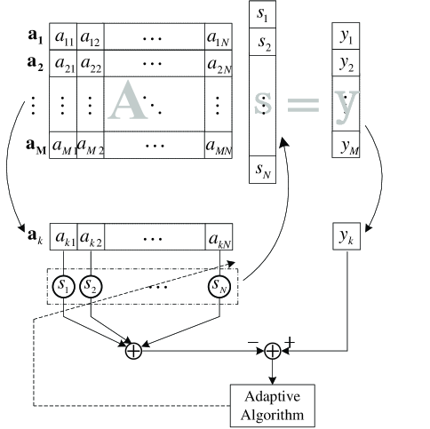
When the above adaptive filtering framework is applied to solve CS problem, there may not be enough data to train the filter coefficients into convergence. Thus, the rows of A and the corresponding elements of y are utilized recursively. The procedures using adaptive filtering framework are illustrated in Fig.1. Suppose that ${\bf s}(n)$ is the updating vector, the detailed update procedures are as follows.

1. Initialize $n=1$, ${\bf s}(0)={\bf 0}$.

2. Send data ${\bf a}_{k}$ and $y_{k}$ to adaptive filter, where

   $$k=\mod(n,M)+1.$$ (13)

3. Use adaptive algorithm to update ${\bf s}(n)$.

4. Judge whether stop condition is satisfied,

   $$\|\textbf{s}(n)-\textbf{s}(n-1)\|_{2}<\varepsilon~{}~{}~{}~{}{\rm or}~{}~{}~{}~{}n>C,$$ (14)

   where $\varepsilon>0$ is a given error tolerance and $C$ is a given maximum iteration number.

5. When satisfied, send ${\bf s}(n)$ back to $\bf s$ and exit; otherwise $n$ increases by one and go back to 2).

Figure 1: The framework of adaptive filter to solve CS reconstruction problem.

Adaptive filtering methods are well-known while CS is a popular topic in recent years, so it is surprising that no literature employs adaptive filtering structure in CS reconstruction problem. The reason might be that the aim of CS is to reconstruct a sparse signal while the solutions to general adaptive filtering algorithms are not sparse. In fact, several LMS variations [43, 44, 45], with some sparse constraints added in their cost functions, exist in sparse system identification. Thus, these methods can be applied to solve CS problem.

In following subsections, $l_{0}$-LMS algorithm and the idea of zero attraction will be firstly introduced. Then $l_{0}$-EFWLMS, which imposes zero attraction on EFW-LMS, is introduced for better performance. Finally, to speed up the convergence of the two new methods, a novel algorithm $l_{0}$-ZAP, which adopts zero attraction in solution space, is further proposed.

2.2 Based on $l_{0}$-LMS algorithm

LMS is the most attractive one in all adaptive filtering algorithms because of its simplicity, robustness and low computation cost. In traditional LMS the cost function is defined as squared error,

$$\xi_{\rm LMS}(n)=|e(n)|^{2}.$$ (15)

Consequently, the gradient descent recursion of the filter coefficient vector is

$${\bf w}(n+1)={\bf w}(n)+\mu e(n){\bf x}(n),$$ (16)

where positive parameter $\mu$ is called step-size.

In order to improve the convergence performance when the unknown parameters are sparse, a new algorithm $l_{0}$-LMS [43] is proposed by introducing a $l_{0}$ norm penalty to the cost function. The new cost function is defined as

$$\xi_{\rm new}(n)=|e(n)|^{2}+\gamma\|{\bf w}(n)\|_{0},$$ (17)

where $\gamma>0$ is a factor to balance the new penalty and the estimation error. Considering that $l_{0}$ norm minimization is an NP hard problem, $l_{0}$ norm is generally approximated by a continuous function. A popular approximation [46] is

$$\|{\bf w}(n)\|_{0}\approx\sum_{i=0}^{L-1}\left(1-{\rm e}^{-\alpha|w_{i}(n)|}\right),$$ (18)

where the two sides of (18) are strictly equal when parameter $\alpha$ approaches infinity. According to (18), the proposed cost function can be rewritten as

$$\xi_{l_{0}-{\rm LMS}}(n)=|e(n)|^{2}+\gamma\sum_{i=0}^{L-1}\left(1-{\rm e}^{-\alpha|w_{i}(n)|}\right).$$ (19)

By minimizing (19), the new gradient descent recursion of filter coefficients is

$$w_{i}(n+1)=w_{i}(n)+\mu e(n)x(n-i)-\kappa\alpha\text{sgn}(w_{i}(n)){\rm e}^{-\alpha|w_{i}(n)|},\quad\forall 0\leq i<L,$$ (20)

where $\kappa=\mu\gamma$ and sgn($\cdot$) is a component-wise sign function defined as

$${\text{sgn}}(x)=\left\{\begin{array}[]{cl}\frac{\textstyle x}{\textstyle|x|}&x\neq 0;\\ 0&{\rm elsewhere}.\end{array}\right.$$ (21)

To reduce the computational complexity of (20), especially that caused by the last term, the first order Taylor series expansion of exponential functions is taken into consideration,

$${\rm e}^{-\alpha|x|}\approx\left\{\begin{array}[]{cl}1-\alpha|x|&|x|\leq\frac{\textstyle 1}{\textstyle\alpha};\\ 0&{\rm elsewhere}.\end{array}\right.$$ (22)

Note that the approximation of (22) is bound to be positive because the value of exponential function is larger than zero. Thus the final gradient descent recursion of filter coefficient vector is

$${\bf w}(n+1)={\bf w}(n)+\mu e(n){\bf x}(n)+\kappa{\bf g}({\bf w}(n)),$$ (23)

where

$${\bf g}({\bf w}(n))=\left[g(w_{0}(n)),g(w_{1}(n)),\ldots,g(w_{L-1}(n))\right]^{\rm T}$$ (24)

and

$$g(x)=\left\{\begin{array}[]{cc}\alpha^{2}x+\alpha&-\frac{\textstyle 1}{\textstyle\alpha}\leq x<0;\\ \alpha^{2}x-\alpha&0<x\leq\frac{\textstyle 1}{\textstyle\alpha};\\ 0&{\rm elsewhere}.\end{array}\right.$$ (25)

The last term of (23) is called zero attraction term, which imposes an attraction to zero on small coefficients. Since zero coefficients are the majority in sparse systems, the convergence acceleration of zero coefficients will improve identification performance. In CS, the zero attraction term will ensure the sparsity of the solution.

By utilizing the correspondence in TABLE 1, the final solution to CS problem can be obtained, which is summarize as Method 1.

Method 1. $l_{0}$-LMS method for CS

1: Initialize ${\bf s}(0)={\bf 0}$, $n$=1, choose $\mu,\alpha,\kappa$;

2: while stop condition (14) is not satisfied;

3:       Determine the input vector ${\bf x}(n)$ and desired signal $d$(n)

$k$ = mod($n,M$)+1;

${\bf x}(n)$ = ${\bf a}_{k}$;

$d(n)$ = $y_{k}$;

4:       Calculate error $e(n)$

$e(n)$ = $d(n)-{\bf x}^{\rm T}(n){\bf s}(n)$;

5:       Update ${\bf s}(n)$ using LMS

${\bf s}(n)$ = ${\bf s}(n-1)+\mu e(n){\bf x}(n)$;

6:       Impose a zero attraction

${\bf s}(n)$ = ${\bf s}(n)+\kappa{\bf g}\left({\bf s}(n-1)\right)$;

7:       Iteration number increases by one

$n=n+1;$

8: End while.

2.3 Based on $l_{0}$-EFWLMS algorithm

Recursive Least Square (RLS) is another popular adaptive filtering algorithm [47], [48], whose cost function is defined as the weighted sum of continuous squared error sequence,

$$\xi_{\rm RLS}(n)=\sum_{i=1}^{n}\lambda^{n-i}|e(i)|^{2}.$$ (26)

where $0\ll\lambda<1$ is called forgetting factor and

$$e(i)=d(i)-{\bf x}^{\rm T}(i){\bf w}(n).$$ (27)

The RLS algorithm is difficult to implement in CS because it costs a lot of computing resources. However, motivated by RLS, the approximation of its cost function with shorter sliding-window is considered, which suggests a new penalty

$$\xi_{\rm EFW-LMS}(n)=\sum_{i=n-Q+1}^{n}\lambda^{n-i}|e(i)|^{2},$$ (28)

where $Q$ is the length of the sliding-window. The algorithm, which minimizes (28), is called Exponentially Forgetting Window LMS (EFW-LMS) [49]. The gradient descent recursion of the filter coefficient vector is

$${\bf w}(n+1)={\bf w}(n)+\mu{\bf X}(n){\bf\Lambda}{\bf e^{\prime}}(n),$$ (29)

where

$${\bf X}(n) =\left[{\bf x}(n-Q+1),{\bf x}(n-Q+2),\ldots,{\bf x}(n)\right],$$ (30)

$${\bf\Lambda} =\left[\begin{array}[]{cccc}\lambda^{Q-1}&0&\ldots&0\\ 0&\lambda^{Q-2}&\ldots&0\\ \vdots&\vdots&\ddots&\vdots\\ 0&0&\ldots&1\end{array}\right],$$ (35)

$${\bf e^{\prime}}(n) =\left[e(n-Q+1),e(n-Q+2),\ldots,e(n)\right]^{\rm T}$$

$$={\bf d^{\prime}}(n)-{\bf X}^{\rm T}(n){\bf w}(n),$$ (36)

and

$${\bf d^{\prime}}(n)=\left[d(n-Q+1),d(n-Q+2),\ldots,d(n)\right]^{\rm T}.$$ (37)

In order to obtain sparse solutions in CS problem, zero attraction is employed again. Thereby the final gradient descent recursion of the filter coefficient vector is

$${\bf w}(n+1)={\bf w}(n)+\mu{\bf X}(n){\bf\Lambda}{\bf e^{\prime}}(n)+\kappa{\bf g}({\bf w}(n)).$$ (38)

This algorithm is denoted as $l_{0}$-EFWLMS.

The method to solve CS problem utilizing the correspondence in TABLE 1 based on $l_{0}$-EFWLMS is summarized in Method 2.

Method 2. $l_{0}$-EFWLMS method for CS

1: Initialize ${\bf s}(0)=0$, choose $Q,\mu,\lambda,\alpha,\kappa$;

2: while stop condition (14) is not satisfied;

3:       Determine $Q$ input vectors ${\bf x}(n-Q+1),\cdots,{\bf x}(n)$

and $Q$ desired signals $d(n-Q+1),\cdots,d(n)$

For $i=n-Q+1,...,n$

$k$ = mod($i,M$)+1;

${\bf x}(i)$ = ${\bf a}_{k}$;

$d(i)$ = $y_{k}$;

End for;

4:       Calculate error vector ${\bf e^{\prime}}(n)$

${\bf e^{\prime}}(n)$ = ${\bf d^{\prime}}(n)-{\bf X}^{\rm T}{\bf s}(n-1)$;

5:       Update ${\bf s}(n)$ using EFW-LMS

${\bf s}(n)$ = ${\bf s}(n-1)+\mu{\bf X}(n){\bf\Lambda}{\bf e^{\prime}}(n)$;

6:       Impose a zero attraction

${\bf s}(n)$ = ${\bf s}(n)+\kappa{\bf g}\left({\bf s}(n-1)\right)$;

7:       Iteration number increases by one

$n=n+1$;

8: End while.

2.4 Based on $l_{0}$-ZAP algorithm

The two methods described above $l_{0}$-LMS and $l_{0}$-EFWLMS can be considered as solutions to $l_{2}-l_{0}$ problem. Observing (23) and (38), it is obvious that both gradient descent recursions are consisted of two parts.

$${\bf w}_{\rm new}={\bf w}_{\rm prev}+{\rm gradient~{}correction}+{\rm zero~{}attraction},$$ (39)

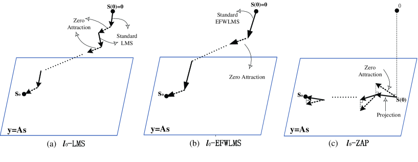
The gradient correction term is to ensure $\bf y=As$, and the zero attraction term is to guarantee the sparsity of the solution. Taking both parts into account, the sparse solution can finally be extracted. The updating procedures of the two methods proposed are shown in Fig.2.(a) and Fig.2.(b). However, convergence of the recursions may be slow because the two parts are hard to balance.

According to the discussions above, CS problem (2) is ill-conditioned and its solution is a $N-M$ subspace. It implies that the sparse solution can be searched iteratively in the solution space in order to speed up convergence. That is, the gradient correction term can be omitted. The updating procedures are demonstrated in Fig.2.(c), where the initial vector of ${\bf s}(0)$ is taken as the Least Square (LS) solution, which belongs to the solution space. Then in iterations, only the zero attraction term is used for updating the vector. The updated vector is replaced by the projection of the vector on solution space as soon as it departs from the solution space. Particularly, suppose ${\bf s}(n)$ is the result gained after $n$th zero attraction, its projection vector in the solution space satisfy the following equation

$$\hat{\bf s}(n)=\arg\min_{{\bf s}^{\prime}(n)}\|{\bf s}^{\prime}(n)-{\bf s}(n)\|_{2}^{2},~{}~{}~{}~{}{\rm s.t.}~{}~{}~{}{\bf A}{\bf s}^{\prime}(n)={\bf y}.$$ (40)

Laplacian Method can be used to solve (40),

$$\hat{\bf s}(n)={\bf s}(n)+{\bf A}^{+}{({\bf y}-{\bf A}{\bf s}(n))},$$ (41)

where ${\bf A}^{+}={\bf A}^{\rm T}{({\bf AA}^{\rm T})}^{-1}$ is the Pseudo-inverse matrix of Least Square. This method is called $l_{0}$-Zero Attraction Projection ($l_{0}$-ZAP), which is summarized in Method 3.

Method 3. $l_{0}$-ZAP method for CS

1: Initialize ${\bf s}(0)={\bf{A^{+}}y}$, choose $\alpha,\kappa$,

2: while stop condition (14) is not satisfied

3:     Update ${\bf s}(n)$ using zero attraction

${\bf s}(n)$ = ${\bf s}(n-1)+\kappa{\bf g}({\bf s}(n-1))$;

4:     Project ${\bf s}(n)$ on the solution space

${\bf s}(n)$ = ${\bf s}(n)+{{\bf A}^{+}}{({\bf y}-{\bf As}(n))}$;

5:     Iteration number increases by one

$n=n+1$;

6: End while

Figure 2: The updating procedures of the three methods, where $\bf s_{o}$ denotes the original signal and ${\bf s}(0)$ denotes the initial value.(a) $l_{0}$-LMS; (b) $l_{0}$-EFWLMS; (c) $l_{0}$-ZAP.

2.5 Discussion

The typical performance of the three proposed methods are briefly discussed here.

• Memory requirement: $l_{0}$-LMS and $l_{0}$-EFWLMS need storage for $\bf y,~{}A$, and $\bf s$, so both their storage requirements are about $MN+M+N$. $l_{0}$-ZAP needs additional storage for, at least, the Pseudoinverse matrix of Least Square, ${\bf A}^{+}$. For large scale situation, $l_{0}$-ZAP requires about twice the memory of the other two algorithms.

• Computational complexity: the total computational complexity depends on the number of iterations required and the complexity of each iteration. First, the complexity of each iteration of these methods will be analyzed. For simplicity, the complexity of each period, instead of that of each iteration, will be discussed. Here, a period is defined as all data in matrix $\bf A$ has been used for one time. For example, in one period, (23) is iterated $M$ times in $l_{0}$-LMS and the projection is used once in $l_{0}$-ZAP. For each period, the complexity of the three methods is listed in TABLE 2. It can be seen that

  $$l_{0}\textrm{-ZAP}<l_{0}\textrm{-LMS}<l_{0}\textrm{-EFWLMS}.$$ (42)

  Table 2: The computational complexity of different method in each period.

  Methods	Multiplications	Additions	Times of Zero Attraction
  $l_{0}$-LMS	$3MN$	$2MN$	$M$
  $l_{0}$-EFWLMS	$(2Q+1)MN$	$(2Q+1)MN$	$M$
  $l_{0}$-ZAP	$2MN$	$2MN+N+M$	$1$

  [1]Please note the computations of zero attraction is not included in the

  above multiplicaitons and additions.

  Second, the number of periods of these methods will be discussed. It is impossible to accurately predict the number of periods of the three proposed methods required to find an approximate solution. However, according to the above discussion, the following equation is always satisfied for the number of periods

  $$l_{0}\textrm{-ZAP}<l_{0}\textrm{-EFWLMS}<l_{0}\textrm{-LMS}.$$ (43)

  Thus, taking both (42) and (43) into consideration, $l_{0}$-ZAP has significantly lower computation complexity than $l_{0}$-LMS and $l_{0}$-EFWLMS. Because $l_{0}$-LMS has lower complexity for each period but larger number of periods than $l_{0}$-EFWLMS, a comparison between $l_{0}$-LMS and $l_{0}$-EFWLMS is hard to make.

• De-noise performance: $l_{0}$-LMS and $l_{0}$-EFWLMS inherit the merit of LMS algorithm that has good de-noise performance. For $l_{0}$-ZAP,

  $$\bf y=As+v=A(s+\hat{v})=A\hat{s}$$ (44)

  where $\bf\hat{v}=A^{+}{v}$ and $\bf v$ is an additive noise. Thus, the iterative vector is not projected on the true solution set $\bf s$ but the solution space $\bf{\hat{s}}$ with additive noise $\bf\hat{v}$. However, we have

  $${\rm E}\left\{{\bf\hat{v}}^{\rm T}{\bf\hat{v}}\right\}\approx\frac{M}{N}{\rm E}\left\{{\bf v}^{\rm T}{\bf v}\right\},$$ (45)

  where ${\rm E}(\cdot)$ denotes the expectation. The proof of (45) is in Appendix A. Equation (45) shows that the power of $\bf\hat{v}$ is far smaller than that of $\bf v$ since $M\ll N$. Moreover, the dimension of $\bf v$ (e.g. $M$) is far smaller than that of $\bf\hat{v}$ (e.g. $N$). Therefore, $l_{0}$-ZAP also has good de-noise performance.

• Implementation difficulty: $l_{0}$-ZAP need two parameters $\alpha$ and $\kappa$, while in $l_{0}$-LMS and $l_{0}$-EFWLMS, there is another parameter $\mu$ to be chosen. Thus, $l_{0}$-ZAP is easier to control than the other two algorithms.

2.6 Some Comments

Comment 1: Besides the proposed $l_{0}$-LMS and $l_{0}$-EFWLMS, the idea of zero attraction can be readily adopted to improve most LMS variants, e.g. Normalized LMS (NLMS), which may be more attractive than LMS because of its robustness. The gradient descent recursion of the filter coefficient vector of $l_{0}$-NLMS is

$${\bf w}(n+1)={\bf w}(n)+\mu\frac{e(n){\bf x}(n)}{\beta+{\bf x}^{\rm T}(n){\bf x}(n)}+\kappa{\bf g}\left({\bf w}(n)\right),$$ (46)

where $\beta>0$ is the regularization parameter. These variants can also improve the performance in sparse signal reconstruction.

Comment 2: Equation (18) is one of the multiple approximations of $l_{0}$ norm. In fact, many other continuous functions can be used for zero attraction. For example, an approximation suggested by Weston et al. [46] is

$$\|{\bf w}\|_{0}\approx\sum_{i=0}^{L-1}\frac{|w_{i}|}{|w_{i}|+\delta},$$ (47)

where $\delta$ is a small positive number. By minimizing (47), the corresponding zero attraction is

$$\kappa{\bf g}({\bf w})=\kappa\left[g(w_{0}),g(w_{1}),\ldots,g(w_{L-1})\right]^{\rm T},$$ (48)

where

$$g(x)=\frac{\delta\text{sgn}(x)}{(|x|+\delta)^{2}}.$$ (49)

This zero attraction term can also be used in the proposed $l_{0}$-LMS, $l_{0}$-EFWLMS and $l_{0}$-ZAP.

3 Convergence analysis

In this section, we will analyse the convergence performance of $l_{0}$-LMS. The steady-state mean square derivation between the original signal and the reconstruction signal will be analyzed and the bound of parameter $\mu$ to guarantee convergence will be deduced.

Theorem 1:Suppose that ${\bf s}$ is the original signal, and $\hat{\bf s}$ is the reconstruction signal by $l_{0}$-LMS, the final mean square derivation in steady state is

$${\rm E}\left\{\|\hat{\bf s}-{\bf{s}}\|_{2}^{2}\right\}=C\left[2\kappa(1-\frac{\mu}{M})a+\kappa^{2}b+\frac{N\mu^{2}}{M}P_{0}\right],$$ (50)

where

$$C = \frac{M^{2}}{2\mu M-(N+2)\mu^{2}};$$ (51)

$$a = {\rm E}\left\{(\hat{\bf s}-{\bf{s}})^{\rm T}{\bf g}(\hat{\bf s})\right\};$$ (52)

$$b = {\rm E}\left\{{\bf g}^{\rm T}(\hat{\bf s}){\bf g}(\hat{\bf s})\right\};$$ (53)

$$P_{0} = {\rm E}\left\{v^{2}\right\},$$ (54)

$P_{0}$ is the power of measurement noise. At the same time, in order to guarantee convergence, parameter $\mu$ should satisfy

$$0<\mu<\frac{2M}{N+2}.$$ (55)

The proof of the theorem is postponed to Appendix B.

As shown in Theorem 1, the final derivation is proportional to $\kappa$ and the power of measurement noise. Thus a large $\kappa$ will result in a large derivation; However, a small $\kappa$ means a weak zero attraction that will induce a slower convergence. Therefore, the parameter $\kappa$ is determined by a trade-off between convergence rate and reconstruction quality in particular applications.

By equation (82) and (83) in appendix we have the following corollary

Corollary 1:The upper bound of derivation is

$${\rm E}\left\{\|\hat{\bf s}-{\bf{s}}\|_{2}^{2}\right\}\leq C\left[2\kappa(1-\frac{\mu}{M})(N+\alpha\|{\bf s}\|_{1})+N\kappa^{2}\alpha^{2}+\frac{N\mu^{2}}{M}P_{0}\right].$$ (56)

The upper bound is a constant under a given signal, thus it can be regarded as a rough criterion to choose the parameters.

4 Experiment Results

The performances of the presented three methods are experimentally verified and compared with typical CS reconstruction algorithms BP[1], SpaRSA[25], GPSR-BB[11], $l1\_ls$[18], Bregman iterative algorithm based on FPC (FPC_AS)[31], IRLS[33] and OMP[36]. In the following experiments, these algorithms are tested with parameters recommended by respective authors. The entries of $M\times N$ sensing matrix $\bf A$ are independently generated from normal distribution with mean zero and variance $1/M$. The locations of $K$ nonzero coefficients of sparse signal $\bf{s}$ are randomly chosen with uniform distribution $[1,N]$. The corresponding nonzero coefficients are Gaussian with mean zero and unit variance. Finally the sparse signal is normalized. The measurements are generated by the following noisy model

$$\bf y=As+v,$$ (57)

where $\bf v$ is an additive white Gaussian noise with covariance matrix ${\sigma}^{2}{\bf I}_{M}$ (${\bf I}_{M}$ is an $M\times M$ identity matrix).

The parameters in stop condition (14) are $\varepsilon=10^{-4}$ for all three methods, $C=10^{5}$ for $l_{0}$-LMS and $l_{0}$-EFWLMS, $C=10^{3}$ for $l_{0}$-ZAP.

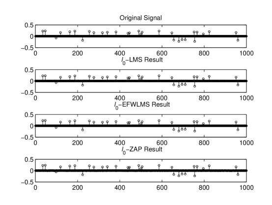
Experiment 1. Algorithm Performance: In this experiment, the performances of the three proposed methods in solving CS problem are tested. The parameters used for the signal model (57) are $\sigma=3.2\times 10^{-3},N=1000,M=200,K=30$. The parameters for the three methods are as follows:

• $l_{0}$-LMS: $\alpha=10$, $\mu=0.1,~{}\kappa=2\times 10^{-6}$;

• $l_{0}$-EFWLMS: $\alpha=10$, $\mu=0.1,~{}\kappa=2\times 10^{-6}$, $Q=4$, $\lambda=0.8$;

• $l_{0}$-ZAP: $\alpha=10$, $\kappa=5\times 10^{-4}$.

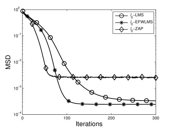
The original signal and the estimation results obtained with $l_{0}$-LMS, $l_{0}$-EFWLMS, and $l_{0}$-ZAP are shown in Fig.3. It can be seen that all three proposed methods reconstruct the original signal. The convergence curves of the three methods are demonstrated in Fig.4, where MSD denotes Mean Square Derivation. For $l_{0}$-LMS and $l_{0}$-EFWLMS, all data of matrix $\bf A$ is used once in each iteration (Please note that the stop condition is not used here). As can be seen in Fig.4, $l_{0}$-EFWLMS has the smallest MSD after convergence and $l_{0}$-ZAP achieves the fastest convergence with sacrifice in reconstruction quality.

To compare with the other algorithms, CPU time is used as an index of complexity, although it gives only a rough estimation of complexity. Our simulations are performed in MATLAB 7.4 environment using an Intel T8300, 2.4GHz processor with 2GB of memory, and under Microsoft Windows XP operating system. The final average CPU time (of total $10$ times, in seconds) and MSD are listed in TABLE 3. Here, the parameter in IRLS is $p=1/2$. It can be seen that the proposed three methods have the least MSD. In addition, $l_{0}$-ZAP is fastest among listed algorithms, though $l_{0}$-LMS and $l_{0}$-EFWLMS have no significant advantage over the other algorithms.

Figure 3: Reconstruction result of the three proposed methods.

Figure 4: Convergence performances of the three proposed methods.

Table 3: The CPU time and MSD.

algorithms	average CPU time (in sec)	MSD
BP	0.582	$1.1\times 10^{-2}$
OMP	0.094	$7.18\times 10^{-2}$
IRLS	1.836	$2.31\times 10^{-3}$
$l1\_ls$	1.436	$7.68\times 10^{-2}$
SpaRSA	0.221	$7.25\times 10^{-2}$
GPSR-BB	0.266	$7.43\times 10^{-2}$
FPC-AS	0.086	$7.38\times 10^{-2}$
$l_{0}$-LMS	1.152	$3.33\times 10^{-4}$
$l_{0}$-EFWLMS	1.544	$2.44\times 10^{-4}$
$l_{0}$-ZAP	0.068	$2.25\times 10^{-3}$

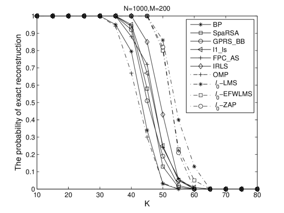
Experiment 2. Effect of Sparsity on the performance: This experiment explores the answer to this question: with the proposed methods, how sparse a source vector $\bf s$ should be to make its estimation possible under given number of measurements. The parameters are the same as the first experiment except that the noise variance is zero. Different sparsities (i.e. $K$) are chosen from $10$ to $80$. For each $K$, $200$ simulations are conducted to calculate the probability of exact reconstruction in different algorithms. The results for all seven algorithms are demonstrated in Fig.5. As can be seen, performances of the three proposed methods far exceed those of the other algorithms. While all the other algorithms fail when sparsity $K$ is larger than $40$, the three methods proposed succeed until sparsity $K$ reaches $45$. In addition, the proposed three methods have similar good performances.

Figure 5: The probability of exact reconstruction versus sparsity $K$.

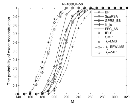
Experiment 3. Effect of number of measurements on the performance: This experiment is to investigate the probability of exact recovery when given different numbers of measurements and a fixed signal sparsity $K=50$. The same setups of the first experiment is used except that the noise variance is zero. Different numbers of measurements $M$ are chosen from $140$ to $320$. All these algorithms are repeated $200$ times for each value of $M$, and the probability curves are shown in Fig.6. Again, it can be seen that the three proposed methods have the best performances. While all other algorithms fail when the measurement number $M$ is lower than $230$, the three proposed methods can still reconstruct exactly the original signal until $M$ reaches $220$. Meanwhile, the proposed algorithms have comparable good performances.

Figure 6: The probability of exact reconstruction versus measurement number $M$.

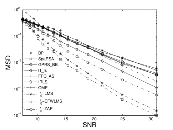
Experiment 4. Robustness against noise: The fourth experiment is to test the effect of signal-to-noise ratio (SNR) on reconstruction performance, where SNR is defined as $\text{SNR}=10\log{\|\bf As\|_{2}^{2}}/{\|\bf v\|_{2}^{2}}$. The parameters are the same as the first experiment and SNR is chosen from $4$dB to $32$dB. For each SNR, all these algorithms are repeated $200$ times to calculate the MSD. Fig.7 shows that the three new methods have better performances than the other traditional algorithms in all SNR. With the same SNR, the proposed algorithms can acquire small MSDs. In addition, the $l_{0}$-EFWLMS has the smallest MSD and $l_{0}$-ZAP has the largest MSD in the three new methods. Obviously, the above results are consistent with discussions in previous sections.

Figure 7: The reconstruction MSD versus SNR.

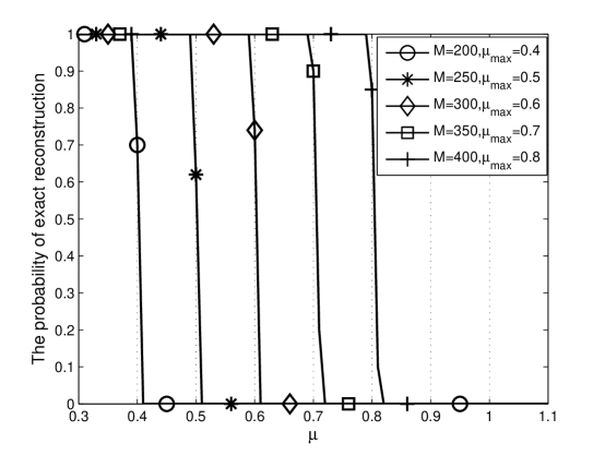
Experiment 5. Effect of parameter $\mu$ on the performance of $l_{0}$-LMS: In this experiment, the condition (55) on step-size to guarantee the convergence of $l_{0}$-LMS will be verified. The setups of this experiment are the same as the first experiment except that $M=\{200,250,300,350,400\}$. For each $M$, $100$ simulations are conducted to calculate the probability of exact reconstruction using $l_{0}$-LMS with the parameters $\alpha=10$, $\kappa=10^{-6}$ and different step-sizes (from 0.3 to 1.1). Fig.8 demonstrates that exact reconstruction cannot be achieved at about $\mu=\{0.4,0.5,0.6,0.7,0.8\}$ with respective $M$ values, which are consistent with the values $\mu_{max}$ calculated by condition (55). This result verifies our derivation in Theorem 1.

Figure 8: The probability of exact reconstruction of $l_{0}$-LMS versus $\mu$ with different $M$.

5 Conclusion

The adaptive filtering framework is introduced at the first time to solve CS problem. Two typical adaptive filtering algorithms $l_{0}$-LMS and $l_{0}$-EFWLMS, both imposing zero attraction method, are introduced to solve CS problem, as well as to verify our framework. In order to speed up the convergence of the two methods, a novel algorithm $l_{0}$-ZAP, which adopts the zero attraction method in the solution space, is further proposed. Thus the mean square derivation of $l_{0}$-LMS in steady state has been deduced. The performances of these methods have been studied experimentally. Compared with those existing typical algorithms, they can reconstruct signal with more nonzero coefficients under a certain given number of measurements; while under a given sparsity, fewer measurements are required by these algorithms. Moreover, they are more robust against noise.

Up to now, there is no theoretical result for determining how to choose the parameters of the proposed algorithms and how much the number of measurements $M$ is in the context of RIP. These remain open problems for our future work. In addition, our future work includes the detailed discussion about the convergence performances of $l_{0}$-EFWLMS and $l_{0}$-ZAP.

Appendix A Proof of (45)

Proof 1

The power of $\bf\hat{v}$ is

$${\rm E}\left\{{\bf\hat{v}}^{\rm T}{\bf\hat{v}}\right\} = {\rm E}\left\{{\bf v}^{\rm T}{(\bf A^{+})}^{\rm T}{\bf A^{+}v}\right\}$$ (58)

$$= {\rm E}\left\{{\bf v}^{\rm T}\left[{\bf A}^{\rm T}{({\bf AA}^{\rm T})}^{-1}\right]^{\rm T}\left[{\bf A}^{\rm T}{({\bf AA}^{\rm T})}^{-1}\right]{\bf v}\right\}$$

$$= {\rm E}\left\{{\bf v}({\bf AA}^{\rm T})^{-1}{\bf v}\right\}$$

$$= {\rm E}\left\{{\bf v}{\rm E}\left\{({\bf AA}^{\rm T})^{-1}\right\}{\bf v}\right\}.$$

where the reason of the last equation of (58) holding is that the noise $\bf v$ and measurement matrix $\bf A$ are independent.

Suppose

$${\bf A}=\left(a_{ij}\right)_{1\leq i\leq M,1\leq j\leq N}$$ (59)

As mentioned in Section I, $a_{ij}$ is i.i.d. with $\mathcal{N}(0,\frac{1}{M})$. Let

$${\bf B}={\bf AA}^{\rm T}=(b_{ij})_{1\leq i\leq M,1\leq j\leq M},$$ (60)

Thus, for the diagonal components,

$$b_{ii}=\sum_{k=1}^{N}{a_{ik}^{2}},1\leq i\leq M.$$ (61)

Since $N$ is very large in CS, according to the central limit theorem [50], the following equation holds approximately,

$$b_{ii}\sim\mathcal{N}\left({\rm E}{b_{ii}},{\rm D}{b_{ii}}\right)=\mathcal{N}\left(\frac{N}{M},\frac{2N}{M^{2}}\right)$$ (62)

where D$\{\cdot\}$ denotes the variance. Similarly, for the non-diagonal components,

$$b_{ij}\sim\mathcal{N}\left({\rm E}{b_{ij}},{\rm D}{b_{ij}}\right)=\mathcal{N}\left(0,\frac{N}{M^{2}}\right),i\neq j.$$ (63)

Because ${N}/{M}\gg{2N}/{M^{2}}$, we have

$${\bf AA}^{\rm T}\approx\frac{N}{M}{\bf I}.$$ (64)

Thus

$$({\bf AA}^{\rm T})^{-1}\approx\frac{M}{N}{\bf I}.$$ (65)

Therefore equation (58) can be simplified as

$${\rm E}\left\{{\bf\hat{v}}^{\rm T}{\bf\hat{v}}\right\}\approx\frac{M}{N}{\rm E}\left\{{\bf v}^{\rm T}{\bf v}\right\}$$ (66)

 

Appendix B Proof of Theorem 1

Proof 2

For simplicity, we use ${\bf w}(n)$, ${\bf x}(n)$, and $d(n)$ instead of ${\bf s}(k)$, ${\bf a}_{k}$ and $y_{k}$, respectively. Suppose that $\bf w_{o}$ is the Wiener solution, thus

$$d(n)={\bf x}^{\rm T}(n){\bf w_{o}}+v(n),$$ (67)

where $v(n)$ is the measurement noise with zero mean. Define the misalignment vector as

$${\bf h}(n)={\bf w}(n)-{\bf w_{o}}.$$ (68)

Thus we have

$$e(n)=v(n)-{\bf x}^{\rm T}(n){\bf h}(n).$$ (69)

Equation (23) is equivalent to

$${\bf h}(n+1)=\left[{\bf I}-\mu{\bf x}(n){\bf x}^{\rm T}(n)\right]{\bf h}(n)+\kappa{\bf g}({\bf w}(n))+\mu v(n){\bf x}(n)$$ (70)

Postmultiplying both sides of (70) with their respective transposes,

$${\bf h}(n+1){\bf h}^{\rm T}(n+1)\!\!\! = \!\!\!\left[{\bf I}-\mu{\bf x}(n){\bf x}^{\rm T}(n)\right]{\bf h}(n){\bf h}^{\rm T}(n)\left[{\bf I}-\mu{\bf x}(n){\bf x}^{\rm T}(n)\right]^{\rm T}$$ (71)

$$+\left[{\bf I}-\mu{\bf x}(n){\bf x}^{\rm T}(n)\right]{\bf h}(n)\kappa{\bf g}({\bf w}(n))$$

$$+\mu v(n)\left[{\bf I}-\mu{\bf x}(n){\bf x}^{\rm T}(n)\right]{\bf h}(n){\bf x}^{\rm T}(n)$$

$$+\kappa{\bf g}({\bf w}(n)){\bf h}^{\rm T}(n)\left[{\bf I}-\mu{\bf x}(n){\bf x}^{\rm T}(n)\right]^{\rm T}$$

$$+\kappa^{2}{\bf g}({\bf w}(n)){\bf g}^{\rm T}({\bf w}(n))$$

$$+\kappa\mu v(n){\bf g}({\bf w}(n)){\bf x}^{\rm T}(n)$$

$$+\mu v(n){\bf x}(n){\bf h}^{\rm T}(n)\left[{\bf I}-\mu{\bf x}(n){\bf x}^{\rm T}(n)\right]^{\rm T}$$

$$+\mu\kappa v(n){\bf x}(n){\bf g}^{\rm T}({\bf w}(n))$$

$$+\mu v^{2}(n){\bf x}(n){\bf x}^{\rm T}(n).$$

Let

$${\bf K}(n)={\rm E}\left\{{\bf h}(n){\bf h}^{\rm T}(n)\right\}$$ (72)

denote a second moment matrix of the coefficient misalignment vector. Taking expectations on both sides of (71) and using the Independence Assumption [48], there is

$${\bf K}(n+1)= {\bf K}(n)-\mu\left({\bf RK}(n)+{\bf K}(n){\bf R}\right)+2\mu^{2}{\bf RK}(n){\bf R}$$

$$+\mu^{2}{\bf R}\text{tr}\left({\bf RK}(n)\right)+2({\bf I}-\mu{\bf R})\kappa{\rm E}\left\{{\bf h}(n){\bf g}^{\rm T}({\bf w}(n))\right\}$$

$$+\kappa^{2}{\rm E}\{{\bf g}\left({\bf w}(n)\right){\bf g}^{\rm T}\left({\bf w}(n)\right)\}+\mu^{2}P_{0}{\bf R},$$ (73)

where

$${\bf R}={\rm E}\left\{{\bf x}(n){\bf x}^{\rm T}(n)\right\}$$ (74)

is the input correlation matrix,

$$P_{0}={\rm E}\left\{v^{2}(n)\right\}$$ (75)

is the minimum mean-squared estimation error and tr$\{\cdot\}$ denotes the trace.

As mentioned in Section I, $\bf A$ is i.i.d. Gaussian with mean zero and variance $1/M$. Then

$${\bf R}=\frac{1}{M}{\bf I}.$$ (76)

Therefore equation (2) can be simplified as

$${\bf K}(n+1)\!\!\! = \!\!\!(1-\frac{2\mu}{M}+\frac{2\mu^{2}}{M^{2}}){\bf K}(n)+\frac{\mu^{2}}{M^{2}}\text{tr}\{{\bf K}(n)\}{\bf I}+2(1-\frac{\mu}{M})\kappa{\rm E}\left\{{\bf h}(n){\bf g}^{\rm T}({\bf w}(n))\right\}$$ (77)

$$+\kappa^{2}{\rm E}\left\{{\bf g}({\bf w}(n)){\bf g}^{\rm T}({\bf w}(n))\right\}+\frac{\mu^{2}}{M}P_{0}{\bf I}.$$

Let

$$D(n)={\rm E}\left\{\|{\bf w}(n)-{\bf w_{o}}\|_{2}^{2}\right\}=\text{tr}\left\{{\bf K}(n)\right\}.$$ (78)

Take the trace on both side of (77),

$$D(n+1)=\left[1-\frac{2\mu}{M}+\frac{(N+2)\mu^{2}}{M^{2}}\right]D(n)+2(1-\frac{\mu}{M})\kappa\alpha(n)+\kappa^{2}\beta(n)+\frac{N\mu^{2}}{M}P_{0},$$ (79)

where

$$\alpha(n)={\rm E}\left\{{\bf h}^{\rm T}({\bf w}(n)){\bf g}({\bf w}(n))\right\};$$ (80)

$$\beta(n)={\rm E}\left\{{\bf g}^{\rm T}({\bf w}(n)){\bf g}({\bf w}(n))\right\}.$$ (81)

Note that both $\alpha(n)$ and $\beta(n)$ are bounded,

$$|\alpha(n)| =\left|{\rm E}\left\{({\bf w}(n)-{\bf w_{o}}){\bf g}({\bf w}(n))\right\}\right|$$

$$\leq{\rm E}\left|\left\{({\bf w}(n)-{\bf w_{o}}){\bf g}({\bf w}(n))\right\}\right|$$

$$\leq\sum_{i=0}^{N-1}{\rm E}\left|\left\{(w_{i}(n)-w_{oi})g(w_{i}(n))\right\}\right|$$

$$=\sum_{|w_{i}(n)|<\frac{1}{\alpha}}{\rm E}\left|(w_{i}(n)-w_{oi})g(w_{i}(n))\right|$$

$$\leq\sum_{|w_{i}(n)|<\frac{1}{\alpha}}{\rm E}\left\{|(w_{i}(n)-w_{oi})||g(w_{i}(n))|\right\}$$

$$\leq\sum_{|w_{i}(n)|<\frac{1}{\alpha}}\alpha{\rm E}\left\{|(w_{i}(n)-w_{oi})|\right\}\quad(\because|g(w_{i}(n))|<\alpha)$$

$$\leq\sum_{|w_{i}(n)|<\frac{1}{\alpha}}\alpha\left\{{\rm E}|w_{i}(n)|+\|{\bf w_{o}}\|_{1}\right\}$$

$$\leq N+\alpha\|{\bf w_{o}}\|_{1};$$ (82)

$$|\beta(n)| =|{\rm E}\left\{{\bf g}^{\rm T}({\bf w}(n)){\bf g}({\bf w}(n))\right\}|$$

$$\leq{\rm E}\left\{|{\bf g}^{\rm T}({\bf w}(n)){\bf g}({\bf w}(n))|\right\}$$

$$\leq\sum_{i=0}^{N-1}{\rm E}\left\{|g(w_{i}(n))|^{2}\right\}$$

$$\leq N\alpha^{2}.$$ (83)

Therefore the following equation should be satisfied to guarantee convergence of (79),

$$|1-\frac{2\mu}{M}+\frac{(N+2)\mu^{2}}{M^{2}}|<1.$$ (84)

We have

$$0<\mu<\frac{2M}{N+2}.$$ (85)

The final mean square derivation in steady state is

$$D(\infty)=C\left[2\kappa(1-\frac{\mu}{M})\alpha(\infty)+\kappa^{2}\beta(\infty)+\frac{N\mu^{2}}{M}P_{0}\right].$$ (86)

where

$$C =\frac{M^{2}}{2\mu M-(N+2)\mu^{2}};$$ (87)

$$\alpha(\infty) ={\rm E}\left\{{\bf h}^{\rm T}({\bf w}(\infty)){\bf g}({\bf w}(\infty))\right\};$$ (88)

$$\beta(\infty) ={\rm E}\left\{{\bf g}^{\rm T}({\bf w}(\infty)){\bf g}({\bf w}(\infty))\right\}.$$ (89)

References

- [1] D. L. Donoho, “Compressed sensing,” IEEE Trans. on Information Theory, 52(4), pp.1289-1306, April 2006.
- [2] E. Candes, J. Romberg, and T. Tao, “Robust uncertainty principles: Exact signal reconstruction from highly incomplete frequency information,” IEEE Trans. Inform. Theory, 52:489-509, 2006.
- [3] Emmanuel Cand s, “Compressive sampling,” Int. Congress of Mathematics, 3, pp.1433-1452, Madrid, Spain, 2006.
- [4] R. G. Baraniuk, “Compressive sensing,” IEEE Signal Processing Magazine, vol.24, no.4, pp.118-122, July 2007.
- [5] M. Lustig, D. Donoho, and J. Pauly, “Sparse MRI: The application of compressed sensing for rapid MR imaging,” Magnetic Resonance in Medicine, 58(6) pp. 1182 - 1195, December 2007.
- [6] S. Kirolos, J. Laska, M. Wakin, et. “Analog-toinformation conversion via random demodulation,” Proc. IEEE Dallas Circuits and Systems Conference, 2006.
- [7] S. S. Chen, D. L. Donoho, and M. A. Saunders, “Atomic decomposition by basis pursuit,” SIAM Journal of Scientific Computing, vol. 20, no. 1, pp. 33-61, 1998.
- [8] S. S. Chen, D. L. Donoho, and M. A. Saunders, “Atomic decomposition by basis pursuit,” SIAM Rev., vol.43, pp.129-159, 2001.
- [9] R. Tibshirani, “Regression shrinkage and selection via the Lasso,” J. Roy. Statist. Soc. B., 58, pp. 267-288, 1996.
- [10] E. van den Berg and M. P. Friedlander, “In Pursuit of a root,” Technical Report TR-2007-19, Department of Computer Science, University of British Columbia, June 2007.
- [11] M. Figueiredo, R. Nowak, and S. Wright, “Gradient projection for sparse reconstruction: application to compressed sensing and other inverse problems,” IEEE Journal on Selected Topics in Signal Processing, vol.1, pp.586 C598, 2007.
- [12] Y. Nesterov and A. Nemirovsky, “Interior-point polynomial methods in convex programming,” Studies in Applied Mathematics, vol.13, 1994, SIAM: Philadelphia, PA.
- [13] D. Luenberger, Linear and Nonlinear Programming, 2nd ed. Reading, MA: Addison-Wesley, 1984.
- [14] C. Johnson, J. Seidel, and A. Sofer, “Interior point methodology for 3-D PET reconstruction,” IEEE Trans. Med. Imag., vol. 19, no. 4, pp. 271 C285, 2000.
- [15] E. Cand s and J. Romberg, “l1-magic: A Collection of MATLAB Routines for Solving the Convex Optimization Programs Central to Compressive Sampling,” 2006 [Online]. Available: www.acm.caltech. edu/l1magic/
- [16] M. Saunders, “PDCO: Primal-Dual Interior Method for Convex Objectives,” 2002 [Online]. Available: http://www.stanford.edu/group/SOL/ software/pdco.html
- [17] C. Paige and M. Saunders, “LSQR: An algorithm for sparse linear equations and sparse least squares,” ACM Trans. Mathemat. Software, vol.8, no.1, pp.43 C71, 1982.
- [18] S. Kim, K. Koh, M. Lustig, S. Boyd, and D. Gorinvesky, “A method for large-scale 1-regularized least squares problems with applications in signal processing and statistics,” Tech. Report, Dept. of Electrical Engineering, Stanford University, 2007. Available at www.stanford.edu/.boyd/l1_ls.html
- [19] M. Osborne, B. Presnell, and B. Turlach, “A new approach to variable selection in least squares problems,” IMA Journal of Numerical Analysis, vol.20, pp.389-403, 2000.
- [20] B. Turlach, “On algorithms for solving least squares problems under an L1 penalty or an L1 constraint,” Proceedings of the American Statistical Association; Statistical Computing Section, pp. 2572-2577, Alexandria, VA, 2005.
- [21] B. Efron, T. Hastie, I. Johnstone, and R. Tibshirani, “Least Angle Regression,” Annals of Statistics, vol.32, pp.407-499, 2004.
- [22] D. Donoho and Y. Tsaig, “Fast solution of l1 -norm minimization problems when the solution may be sparse,” Manuscript 2006 [Online]. Available: http://www.stanford.edu/
- [23] J. Friedman, T. Hastie, and R. Tibshirani, “Pathwise Coordinate Optimization,” 2007 [Online]. Available: www-stat.stanford. edu/hastie/pub.htm
- [24] E. Hale, W. Yin, and Y. Zhang, “A fixed-point continuation method for l1 regularized minimization with applications to compressed sensing,” Manuscript 2007 [Online]. Available: http://www.dsp.ece.rice.edu/cs/
- [25] S. Wright, R. Nowak, and M. Figueiredo, “Sparse reconstruction by separable approximation,” ICASSP’08, 2008.
- [26] G. Narkiss and M. Zibulevsky, “Sequential Subspace Optimization Method for Large-Scale Unconstrained Problems The Technion,” Haifa, Israel, Tech. Rep. CCIT No.559, 2005.
- [27] M. Figueiredo and R. Nowak, “A bound optimization approach to wavelet-based image deconvolution,” Proc. IEEE Int. Conf. Image Processing (ICIP), 2005, pp.782 C785.
- [28] I. Daubechies, M. Defrise, and C. De Mol, “An iterative thresholding algorithm for linear inverse problems with a sparsity constraint,” Commun. Pure Appl. Mathe., vol.57, pp.1413 C1541, 2004.
- [29] Y. Nesterov, “Gradient methods for minimizing composite objective function,” CORE Discussion Paper 2007/76 [Online]. Available: http://www.optimization-online.org/DB_HTML/2007/09/1784.html
- [30] J. F. Cai, S. Osher, and Z. Shen, “Linearized bregman iterations for compressive sensing,” Mathematics of Computations, vol.78, pp.1515-1536, Oct. 2008.
- [31] W. Yin, S. Osher, D. Goldfarb, and J. Darbon, “Bregman iterative algorithm for l1-minimization with applications to compressive sensing,” SIAM J. Imaging Sciences, vol. 1, no. 1, pp. 143-168, 2008.
- [32] I. F. Gorodnitsky and B. D. Rao, “Sparse signal reconstruction from limited data using FOCUSS: A re-weighted minimum norm algorithm,” IEEE Trans. Signal Processing, vol.45 pp. 600-616, Mar. 1997.
- [33] R. Chartrand and W. Yin, “Iteratively reweighted algorithms for compressive sensing,” ICASSP, pp. 3869-3872, April 2006.
- [34] I. Daubechies, R. DeVore, M. Fornasier, et.al., “Iteratively re-weighted least squares minimization for sparse recovery.” Communications on pure and applied mathematics, vol. 63, no. 1, pp.1-38, 2010.
- [35] Y. C. Pati, R. Rezaiifar, and P. S. Krishnaprasad, “Orthogonal matching pursuit: Recursive function approximation with applications to wavelet decomposition,” Proc. 27th Annu. Asilomar Conf. Signals, Systems, and Computers, Pacific Grove, CA, Nov. 1993, vol. 1, pp. 40-44.
- [36] J. Tropp and A. Gilbert, “Signal recovery from random measurements via orthogonal matching pursuit,” IEEE Trans. on Information Theory, 53(12), pp. 4655-4666, Dec. 2007.
- [37] D. L. Donoho, Y. Tsaig, and Jean-Luc Starck, “Sparse solution of underdetermined linear equations by stagewise orthogonal matching pursuit,” Technical report, Mar. 2006.
-
[38]
D. Needell, and R. Vershynin, “Signal recovery from incomplete and
inaccurate measurements via regularized orthogonal matching
pursuit,” 2007 [Online]. Available:
http://www-stat.stanford.edu/
~dneedell/papers/ROMP-stability.pdf. - [39] W. Dai, and O. Milenkovic, “Subspace pursuit for compressive sensing: Closing the gap between performance and complexity,” arXiv:0803.0811v3 [CS.NA], Jan. 2009.
- [40] D. Needell and J. A. Tropp, “Cosamp: Iterative signal recovery from incomplete and inaccurate samples.” Applied and Computational Harmonic Analysis, vol. 26, no.3, pp. 301-321, May 2009.
- [41] T. Blumensath and M. E. Davies, “Iterative hard thresholding for compressed sensing,” Applied and Computational Harmonic Analysis, vol. 27, no. 3, pp. 265-274, 2009.
- [42] J. Trzasko and A. Manduca, “Highly Undersampled Magnetic Resonance Image econstruction via Homotopic l0-Minimization,” IEEE Transactions on Medical Imaging, vol. 28, no. 1, Jan. 2009.
- [43] Y. Gu, J. Jin, and S. Mei, “l0 Norm Constraint LMS Algorithm for Sparse System Identification,” IEEE Signal Processing Letters,vol. 16, no. 9,pp. 774-777, Sep. 2009.
- [44] J. Benesty and S. L. Gay, “An improved PNLMS algorithm”, Proc. IEEE ICASSP, 2002, pp. II-1881-II-1884.
- [45] R. K. Martin, W. A. Sethares, et al., “Exploiting sparsity in adaptive filters”, IEEE Trans. Signal Processing, vol. 50, pp. 1883-1894, Aug. 2002.
- [46] J. Weston, A. Elisseeff, B. Scholkopf, et, “Use of zero-norm with linear models and kernel methods,” JMLR special Issue on Variable and Feature Selection, pp.1439-1461, 2002.
- [47] C F. N. Cowan and P. M. Grant, Adaptive Filters. Englewood Cliffs, NJ: Prentice-Hall, 1985.
- [48] S. Haykin, Adaptive Filter Theory. Englewood Cliffs, NJ: Prentice-Hall, 1986.
- [49] G. Glentis, K. Berberidis, S. Theodoridis, “Efficient least squares adaptive algorithms for FIR transversalfiltering,” IEEE signal processing magazine, vol. 16, no. 4, pp.13-41, 1999.
- [50] O. Kallenberg, Foundation of Modern Probability, 2nd ed. Springer, NY, 2002.