USLV: Unspanned Stochastic Local Volatility Model

Abstract

We propose a new framework for modeling stochastic local volatility, with potential applications to modeling derivatives on interest rates, commodities, credit, equity, FX etc., as well as hybrid derivatives. Our model extends the linearity-generating unspanned volatility term structure model by Carr et al. (2011) by adding a local volatility layer to it. We outline efficient numerical schemes for pricing derivatives in this framework for a particular four-factor specification (two “curve” factors plus two “volatility” factors). We show that the dynamics of such a system can be approximated by a Markov chain on a two-dimensional space $(Z_{t},Y_{t})$, where coordinates $Z_{t}$ and $Y_{t}$ are given by direct (Kroneker) products of values of pairs of curve and volatility factors, respectively. The resulting Markov chain dynamics on such partly “folded” state space enables fast pricing by the standard backward induction. Using a nonparametric specification of the Markov chain generator, one can accurately match arbitrary sets of vanilla option quotes with different strikes and maturities. Furthermore, we consider an alternative formulation of the model in terms of an implied time change process. The latter is specified nonparametrically, again enabling accurate calibration to arbitrary sets of vanilla option quotes.

1 Introduction

1.1 Motivation

The present work is motivated by the desire to have a unified modeling methodology and shared implementation for derivatives pricing with a dynamic volatility smile for various asset classes, including interest rates (IR), commodities, equities, credit, foreign exchange (FX) etc., as well as for modeling hybrid derivatives such as equity-IR or equity-commodities hybrids. We present one possible approach, which extends a recently proposed class of stochastic volatility models.

1.2 Related Previous Work

Gabaix, (2007) proposed a new class of asset price models, the so-called linearity-generating processes (LGP). Such processes are defined by the condition that the current prices of basic instruments (stock, bonds, futures, swaps etc.) are linear in a driving Markov process $X_{t}$. This stands in sharp contrast to popular affine models where, e.g., a zero-coupon bond price $P(t,T)$ is an exponentially-affine function of a Markov driver $X_{t}$.

On the theoretical side, the LGP processes appear very attractive. Indeed, typical ways we model basic instruments are drastically different between, say, IR and equity models. In the equity world, basic instruments (equities) are linear in stochastic factors (usually taken to be equity prices themselves for purposes of modeling derivatives), and volatility is stochastic (SV) and unspanned (USV, see below for the definition of this term).

In the IR world, the mathematics are almost the same for the HJM-type models that model the entire yield curve. As the yield curve is in one-to-one correspondence with bond prices, it can be viewed as an “observable” basic instrument that again is linear in factors, and typically gives rise to USV.

But such linearity of HJM-like models has a high price, namely that the number of state variables needed for the Markovian dynamics turns out to be too high for use in a lattice-based setting in most cases of practical interest. Therefore, even with Markovian specifications, HJM-like models are typically employed within a Monte Carlo setup rather than on a lattice. On the other hand, an attempt to reduce the curve modeling to a short-rate modeling, as is done in affine models, leads to a nonlinear relation between bond prices and the factors, which produces undesirable side effects, such as a dependence of the instantaneous forward curve on the short-rate volatility.

This problem is resolved in the LGP approach. By putting both equity and bonds on equal footing in terms of making them both linear functionals of the factors (and doing it in a different way from HJM), the LGP-based models play a role of “grand unification models,” similar in a conceptual sense to “grand unification theories” (GUT) in physics. No proliferation of the number of Markov drivers occurs in LGP-type models as we move from one class of basic instruments (stocks) to other class (bonds).

Also on the practical side, linearity has profound consequences for tractability of asset pricing modeling within the LGP framework. In particular, if a zero-coupon bond price is linear in $X_{t}$, then so will be prices of a coupon bond or a swap. As a result, the swaption pricing, e.g. can be done in a semi-analytical form without additional approximations, such as those used by the Libor Market Models (LMM). It is also very helpful in calibration, as will be discussed in more detail below.

To summarize, the class of LGP-like models identified by Gabaix is a new interesting class that may develop into a viable competitor to both affine models, which are currently one of the main workhorses for derivatives modeling in credit, commodities, rates and other asset classes, and also HJM-type models. Yet this approach is in its infancy compared to the well-studied class of affine models.

In 2011, Carr, Gabaix and Wu (CGW) proposed a LGP-type stochastic volatility term structure model (Carr et al., (2011)). CGW, in particular, emphasize the point that stochastic volatility generated in LGP-type models is unspanned in the sense of the definition of Colin-Dufresne & Goldstein, (2002), who coined the original term “unspanned volatility”. The CGW model offers a number of attractive features. Most importantly, it is a low-dimension Markov model with unspanned stochastic volatility (USV), and an orthogonal set of model parameters with a separate calibration to the term structure and option volatilities.

The CGW model is a pure stochastic volatility model, as volatility is modeled as a superposition of CIR processes. To make it more practical, it would be very useful to add a local volatility layer to the model. Our extension of the CGW model amounts to introduction of such a local volatility factor, along with efficient numerical methods for calibration and pricing. To differentiate our framework from CGW, in what follows we will refer to it as the unspanned stochastic local volatility (USLV) model.

2 Overview of Our Framework

By construction, USLV preserves the linearity and USV properties of the CGW approach. Another property inherited from the CGW model is that USLV is formulated directly in the physical measure $\mathbb{P}$ (see below) rather than in the risk-neutral measure $\mathbb{Q}$, which makes it easier, e.g., to combine the historical and pricing data for model estimation, if desired.

The main theoretical construction that USLV adds to the CGW model is a local volatility layer. The resulting mixed stochastic/local volatility dynamics has a few important implications.

First, adding a local volatility layer enables nearly perfect matching of an arbitrary number of European vanilla option quotes with different strikes and maturities. Such an extension is clearly desirable in order to apply this approach for pricing of both vanilla and exotic derivatives, especially if vanilla options are used to hedge the exotics.

Second, the presence of a local volatility layer alongside a stochastic volatility part induces a decomposition of the option volatility into spanned and unspanned parts, rather than being of a pure unspanned type as in the CGW model. One could expect that such decomposition of volatility should translate into a decomposition of an option’s vega into a delta-vega and a “genuine vega” part.

Because of the way our model is calibrated, it enables traders to incorporate their view on the relative weights of the spanned and unspanned parts in the option’s vegas. By viewing a trader’s inputs as a prior model that does not necessarily match observed options, our model finds a minimal adjustment (“tweak”) to the trader’s prior model in order to reinforce an accurate match of the option quotes.

In contrast, the volatility in local volatility models would be 100% spanned. In local volatility models, matching vanilla pricing would fix the volatility surface for all strikes and maturities, and would not leave any flexibility for the model to match prices of more exotic options. The inclusion of stochastic volatility allows one to simultaneously have more realistic forward smile dynamics and additional parameters to match exotics’ prices (if available). The ability of USLV to incorporate a possible trader’s view is what sets it apart from both pure local volatility models and pure SV models of the CGW type.

On the implementation side, USLV concentrates on the most important low-dimensional specifications for practicality, e.g., two factors for the term structure (with $N$ curve factors in general), and one or two factors for stochastic volatility (with $M$ volatility factors in general). In particular, for a (2+2)-factor case, we show how to approximate the dynamics of the driving factors by a two-dimensional Markov chain on a space constructed by folding (see below) of the original four-dimensional state space. This enables fast pricing by standard backward induction on the chain.

It should be noted that while in this paper we concentrate on modeling term-structure dynamics (e.g., of futures, swap rates or credit spreads) with potential applications to “term structure asset classes,” such as IR, commodities or credit, the same approach can be used for modeling spot prices, which would be a proper setting for “spot asset classes,” such as equities or FX. Moreover, due to a symmetric treatment of “term-structure assets” and “spot assets” in the present framework, this approach is readily available for modeling hybrid derivative products (e.g., equity-IR or equity-commodity hybrids) using the same implementation. Changes from one asset class to another would amount to a proper reparametrization and reinterpretation of the Markov generator matrices while leaving the computational algorithm intact. Furthermore, in the continuous limit, different parametrizations of the stochastic volatility generator in our Markov chain model give rise to a rich class of (2+2)-factor models, including stochastic local volatility with jumps. Note that in this paper we primarily concentrate on specifications whose continuous limit is a two-dimensional diffusion with a two-dimensional diffusive stochastic local volatility. This case is covered in detail below in Sect. 6. However, in Sect. 7, we will present an alternative formulation that can give rise to jumps in both the underlying and stochastic volatility. Our approach is thus quite flexible in its ability to accommodate different specifications of the dynamics, including a four-factor stochastic local volatility model with jumps.

2.1 USLV vs. HJM vs. Affine Models

Our initial interest in using LGP-type models for modeling stochastic volatility was inspired by the observation that LGP-type models (and, by extension, USLV-like models) seem to combine the best features of both HJM-type models and affine models, while avoiding their disadvantages. Indeed, like the HJM-type models, the stochastic volatility is unspanned in USLV. Unlike the HJM-types, the model is Markov in dimension $N+M$ rather than $N+N(N+1)/2+M$, as in HJM-type models. Conversely, both affine models and USLV have the same number of state variables ($N+M$). However, in USLV, volatility is always (partly) unspanned, while in affine models, volatility in general will be spanned unless some special constraints are imposed on parameters, which might be restrictive for calibration purposes. (See also Table 1 below.)

The above reasoning suggests that if we manage to generalize the pure stochastic volatility model of CGW to a stochastic local volatility model (i.e., to make a USLV out of CGW), and do it in a numerically efficient way, and if the resulting model demonstrates good parameters and hedges stability etc., then such a model can be considered a viable candidate for use in practice. This paper outlines the theoretical framework for USLV, leaving numerical experiments for future work.

A few more words of caution are in order here. Our outline of the USLV is generic and is not tied yet to any specific asset class. Each asset class makes its own demands on a model. For example, the ability to reproduce the Samuelson effect and asset cointegration are very important for commodities, alongside the ability to handle seasonality in asset levels and volatilities for certain commodities, such as gas or power. It has yet to be seen how (or whether) the USLV framework can accommodate such specific requirements. A discussion of this matter is planned for the second stage of the present theoretical work.

A brief summary of different model classes is presented in Table 1, where we compare the behavior of equity stochastic volatility models such as the Heston model, HJM-type, affine-type and LGP/CGW/USLV-type. The third column shows the functional form of conditional expectations arising in calculation of prices of elementary instruments.

Model	$BI_{t}$	$BV_{t}$	$BI_{t}=f(BV_{t})$	USV	D
Equity	$S_{t}$	$S_{t},Y_{t}$	$f(S_{t},Y_{t})=S_{t}$	Yes	$1+M$
IR HJM	$P_{t}^{T}$	$P_{t}^{T},Y_{t}$	$f(P_{t}^{T},Y_{t})=P_{t}^{T}$	Yes	$N+N(N+1)/2+M$
IR Affine	$P_{t}^{T}$	$X_{t},Y_{t}$	$f(X_{t},Y_{t})$	No	$N+M$
CGW/USLV	$P_{t}^{T}$	$X_{t},Y_{t}$	$f(X_{t},Y_{t})=\alpha_{tT}X_{t}+\beta_{tT}$	Yes	$N+M$

Table 1: Model comparison summary. Note that “Yes” in column USV for IR HJM means “in general, yes,” and likewise “No” for IR Affine means “in general, no, unless special ’knife-edge’ constraints are imposed on parameters of the model.” Here $S_{t},P_{t}^{T}$ and $Y_{t}$ stand for the stock and bond prices and volatility factor, respectively, while $BI_{t}$ and $BV_{t}$ stand for basic instruments and basic variables, respectively. Finally, $D$ stands for for the total number of state variables needed for a Markovian description.

3 The Carr-Gabaix-Wu Model

In this section, we provide a brief overview of the CGW model of Carr et al., (2011). The CWG model is then used as the first step in our setting. Simultaneously, in this section we set our notation, on which we largely follow Carr et al., (2011).

3.1 State-Price Processes and Martingale Pricing

The famous fundamental theorem of asset pricing (Harrison & Pliska, (1981)) states that if the economy is arbitrage free, then there exists (under certain technical conditions such as positivity and time consistence) a strictly positive process $M_{t}$ called the state space deflator, such that the deflated gain process associated with any admissible trading strategy is a martingale under the measure $\mathbb{P}$. In particular, for a contingent payoff $\Pi_{T}$ at time $T>t$, its value at time $t$ is given by the following $\mathbb{P}$-conditional expectation:

$$V(t,T)=\mathbb{E}_{t}\left[\frac{M_{T}}{M_{t}}\Pi_{T}\right]$$ (1)

The ratio $M_{T}/M_{t}$ is sometimes referred to as the stochastic discount factor or the pricing kernel. The $\mathbb{P}$-measure SDE for $M_{t}$ reads

$$\frac{dM_{t}}{M_{t}}=-rdt-\boldsymbol{\lambda}(t,{\bf Z}_{t})d{\bf Z}_{t},$$

where ${\bf Z}_{t}$ is a vector of risk factors and $\boldsymbol{\lambda}(t,{\bf Z}_{t})$ measures the market prices of risk for these factors. The formal solution to this SDE takes a multiplicative form

$$M_{t}=M_{0}\exp\left(-\int_{0}^{t}r_{s}ds\right)\mathcal{E}\left(-\int_{0}^{t}\lambda(t,Z_{s})dZ_{s}\right),$$

where $\mathcal{E}(\cdot)$ stands for the stochastic exponential martingale operator. The latter defines the Radon-Nikodým derivative $d\mathbb{Q}/d\mathbb{P}$ that transforms the physical measure $\mathbb{P}$ to the risk-neutral measure $\mathbb{Q}$ such that, under $\mathbb{Q}$, the contingent claim valuation reads

$$V(t,T)=\mathbb{E}_{t}^{\mathbb{Q}}\left[\exp\left(-\int_{t}^{T}r_{s}ds\right)\Pi_{T}\right].$$ (2)

3.2 One-Factor Case

Our starting point is a version of one-factor LGP dynamics suggested in Bekker & Bouwman, (2009). It differs from Carr et al., (2011) by i) parametrization, and ii) derivation and interpretation of the main result of the LGP approach (see Eq.(9) below). The two formulations can, however, be mapped onto one another by a proper re-parametrization.

Assume that a state variable $X_{t}$ is driven by the following SDE under measure $\mathbb{P}$:

$$dX_{t}=r_{t}X_{t}dt+\sigma(t,X_{t})\left[\lambda(t,X_{t})dt+dW_{t}\right],$$ (3)

where $W_{t}$ is the standard Brownian motion and the short rate $r_{t}$ is an affine function of $X_{t}$:

$$r_{t}=a-ce^{-\mu t}X_{t}\equiv a-c\tilde{X}_{t}$$ (4)

where $\tilde{X}_{t}=e^{-\mu t}X_{t}$ is a detrended state variable with $\mu$ being the growth rate of $X_{t}$, and $a>0$ and $c>0$ are two constants.

The $\mathbb{P}$-measure SDE for the state price deflator $M_{t}$ reads

$$\frac{dM_{t}}{M_{t}}=-r_{t}dt-\lambda(t,X_{t})dW_{t}$$ (5)

The representation of stochastic dynamics given in Eq.(3) and Eq.(5) is convenient as both the real world (measure $\mathbb{P}$) and risk-neutral (measure $\mathbb{Q}$) dynamics can be directly read from these equations provided we know functions $\sigma(t,X_{t})$ and $\lambda(t,X_{t})$. Indeed, by the Girsanov theorem, the combination $dW_{t}+\lambda(t,X_{t})dt$ is a $\mathbb{Q}$-martingale, so that the $\mathbb{Q}$-measure drift of $X_{t}$ is the short rate $r_{t}$. This means that the state variable $X_{t}$ can be interpreted economically as a risky (tradable or non-tradable) asset, or be related to aggregate market returns, see Bekker & Bouwman, (2009).

Using Eq.(5) and the fact that $M_{t}X_{t}$ is a martingale under measure $\mathbb{P}$ (which is easy to verify using Itó’s lemma and Eq.(3) and Eq.(5)), we compute the conditional time-$t$ expectation of $M_{T}$ as follows:

$$\mathbb{E}_{t}\left[M_{T}\right] = \mathbb{E}_{t}\left[M_{t}-\int_{t}^{T}r_{s}M_{s}ds-\int_{t}^{T}\lambda(s,X_{s})M_{s}dW_{s}\right]$$

$$= M_{t}-\int_{t}^{T}a\mathbb{E}_{t}\left[M_{s}\right]ds+\int_{t}^{T}ce^{-\mu s}\mathbb{E}_{t}\left[M_{s}X_{s}\right]ds$$

$$= M_{t}-\int_{t}^{T}a\mathbb{E}_{t}\left[M_{s}\right]ds+\left(\int_{t}^{T}ce^{-\mu s}ds\right)M_{t}X_{t}$$

This produces the following result for the time-$t$ zero-coupon bond price

$$P(t,T)=\frac{\mathbb{E}_{t}\left[M_{T}\right]}{M_{t}}=1-\int_{t}^{T}aP(t,s)ds+\left(\int_{t}^{T}ce^{-\mu s}ds\right)X_{t}$$ (7)

Differentiating this relation with respect to $T$, we transform it into a differential equation:

$$\frac{\partial P(t,T)}{\partial T}=-aP(t,T)+ce^{-\mu T}X_{t}$$ (8)

whose solution reads (Bekker & Bouwman, (2009))

$$P(t,T)=e^{-a\tau}\left[1+ce^{-\mu t}\frac{e^{(a-\mu)\tau}-1}{a-\mu}X_{t}\right]=e^{-a\tau}\left[1+c\frac{e^{(a-\mu)\tau}-1}{a-\mu}\tilde{X}_{t}\right]\,,\;\;\tau=T-t$$ (9)

Note that this expression does not depend on specification of functions $\sigma(t,X_{t})$ and $\lambda(t,X_{t})$ in Eq.(3), and the shape of the yield curve at time $t$ is driven by the current value of $X_{t}$. This is different from affine models where the bond price is represented as a conditional expectation of a non-linear functional of future values of the state variables.

The solution of Eq.(3) in the zero volatility limit $\sigma(t,X_{t})=0$ reads

$$X_{t}=\left\{\begin{array}[]{lll}\frac{\displaystyle a-\mu}{\displaystyle c}\frac{e^{\mu t}}{1-\eta_{0}e^{-(a-\mu)t}},&\eta_{0}=1-\frac{a-\mu}{cX_{0}},&\mbox{if }\mu\neq a,\\ \frac{\displaystyle e^{\mu t}}{\displaystyle\eta_{0}+ct},&\eta_{0}=\frac{1}{X_{0}},&\mbox{if }\mu=a\end{array}\right.$$ (12)

In what follows, we concentrate on the case $\mu<a$ which corresponds to the scenario where the detrended asset $\tilde{X}_{t}=e^{-\mu t}X_{t}$ reaches a constant level $\tilde{X}_{\infty}=\frac{a-\mu}{c}>0$ as $t\rightarrow\infty$. In addition, we assume that $X_{0}>\frac{a-\mu}{c}$, so that $0<\eta_{0}<1$ which produces an increasing and concave yield curve, while negative values of $\eta_{0}$ produce inverted yield curves, see Fig. 1.

Figure 1: Yield curves obtained with a one-factor specification Eq.(9) with $t=0$ for different combinations of parameters $a,\,\mu$ and $\eta_{0}$, as a function of maturity in years. Parameter $c$ equals 0.1 for all curves.

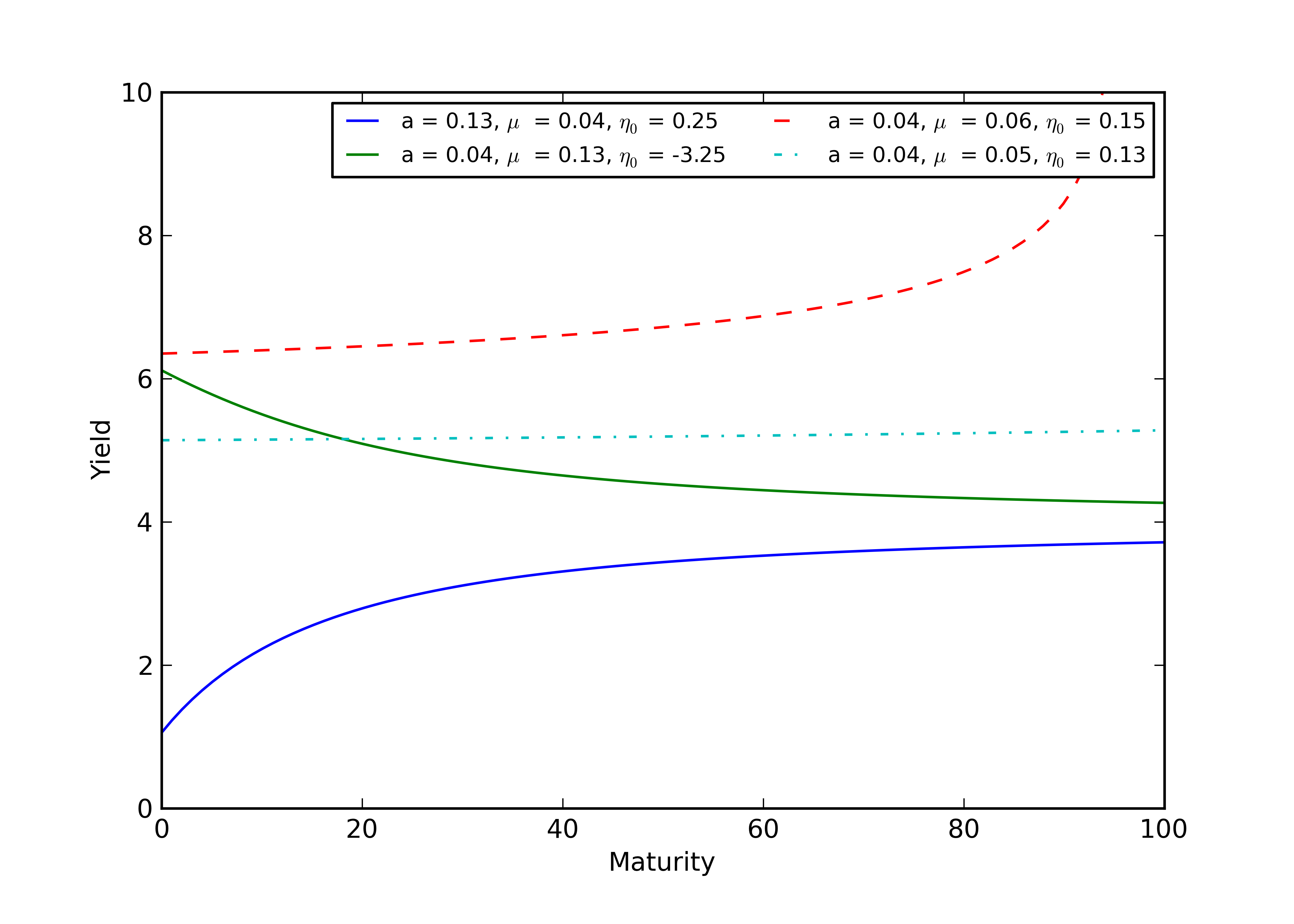
In this scenario, the short rate $r_{t}$ approaches $\mu$ as $t\rightarrow\infty$. If $\eta_{0}$ satisfies a more restrictive constraint $\eta_{0}<\mu/a$, then the short rate $r_{t}$ stays positive (or equivalently $P(t,T)\leq 1$) for all $t$. Therefore, we assume a slightly more general constraint on $\eta_{0}$ by introducing another parameter $\bar{\mu}$ that lies in the interval $[\mu,a]$:

$$0\leq\eta_{0}<\frac{\bar{\mu}}{a}\;,\;\;\mu\leq\bar{\mu}\leq a$$ (13)

For such choice of $\eta_{0}$, Eq.(12) with $\mu<a$ produces a concave and monotonically increasing yield curve, while the short rate $r_{t}$ and state process $X_{t}$ are bounded at all times as follows:

$$a-\frac{a-\mu}{1-\left(\bar{\mu}/a\right)e^{-(a-\mu)t}}\leq r_{t}\leq\mu,\qquad\frac{a-\mu}{c}\leq\tilde{X}_{t}\leq\frac{a-\mu}{c}\frac{1}{1-\left(\bar{\mu}/a\right)e^{-(a-\mu)t}}$$ (14)

where the low and upper boundaries for $r_{t}$ (respectively, upper and lower boundaries for $\tilde{X}_{t}$) are attained by setting $\eta_{0}=\bar{\mu}/a$ or $\eta_{0}=0$, respectively. One sees that parameter $\bar{\mu}$ can be used to control how much the short rate $r_{t}$ can go negative. If we set $\bar{\mu}=\mu$, the short rate $r_{t}$ is non-negative at all times $t\geq 0$, but as we will see shortly such choice for $\bar{\mu}$ may not necessarily be optimal in the present framework.

Now we return to Eq.(3) with non-vanishing volatility, and consider the following ansatz for $X_{t}$:

$$X_{t}=\frac{a-\mu}{c}\frac{e^{\mu t}}{1-Y_{t}e^{-(a-\mu)t}}\,,\;\;\mu<a$$ (15)

which is obtained by replacing a constant $\eta_{0}$ in Eq.(12) by a stochastic process $Y_{t}$ restricted to the strip $[0,\bar{\mu}/a]$. Such a process with a given initial value $0\leq Y_{0}\leq\bar{\mu}/a$ can be constructed as follows:

$$Y_{t}=\frac{\bar{\mu}Y_{0}}{aY_{0}+(\bar{\mu}-aY_{0})Z_{t}}$$ (16)

where $Z_{t}\geq 0$ is a non-negative martingale under measure $\mathbb{P}$ that starts at $Z_{0}=1$ and satisfies the following SDE:

$$\frac{dZ_{t}}{Z_{t}}=-\hat{\sigma}(t,Z_{t})dW_{t}$$ (17)

where $\hat{\sigma}(t,Z_{t})$ is a local volatility function that will be specified later. The initial value $X_{0}$ is expressed in terms of $Y_{0}$ as follows:

$$X_{0}=\frac{a-\mu}{c}\frac{1}{1-Y_{0}}$$ (18)

Substituting Eq.(16) into Eq.(15), we obtain

$$X_{t}=\frac{a-\mu}{c}\frac{e^{\mu t}\left[aY_{0}+\left(\bar{\mu}-aY_{0}\right)Z_{t}\right]}{aY_{0}\left[1-(\bar{\mu}/a)e^{-(a-\mu)t}\right]+\left(\bar{\mu}-aY_{0}\right)Z_{t}}\equiv\frac{a-\mu}{c}e^{\mu t}\frac{\left(\alpha+\beta Z_{t}\right)}{\alpha\kappa(t)+\beta_{0}Z_{t}}$$ (19)

where

$$\alpha=aY_{0}\;,\;\;\beta=\bar{\mu}-\alpha\;,\;\;\kappa(t)=1-\frac{\bar{\mu}}{a}e^{-(a-\mu)t}$$ (20)

Eq.(19) defines $X_{t}$ as a fractional-linear function of the martingale process $Z_{t}$ determined by Eq.(17). Clearly, the process $X_{t}$ defined by Eq.(19) is bounded, as it should be as long as it is related by a linear equation Eq.(9) to the bond price which is bounded. By taking the limits $Z_{t}\rightarrow 0$ and $Z_{t}\rightarrow\infty$, one obtains bounds for $\tilde{X}_{t}$:

$$\frac{a-\mu}{c}\leq\tilde{X}_{t}\leq\frac{a-\mu}{c}\frac{1}{1-(\bar{\mu}/a)e^{-(a-\mu)t}}$$ (21)

which coincides with Eq.(14). Note that Carr et al., (2011) obtain a fractional-linear expression for $X_{t}$ as a function of $Z_{t}$ that is similar to our Eq.(19), however their choice of time-dependent coefficients is different.

Using Ito’s lemma, we find that $X_{t}$ defined by Eq.(19) satisfies Eq.(3) provided we choose the following specification for functions $\sigma(t,X_{t})$ and $\lambda(t,X_{t})$ (which we express here as functions of $Z_{t}$ rather than $X_{t}$):

$$\sigma(t,X_{t}) = \alpha\hat{\sigma}(t,Z_{t})\frac{\bar{\mu}}{a}\frac{a-\mu}{c}\frac{\beta Z_{t}e^{-(a-2\mu)t}}{\left[\alpha\kappa(t)+\beta Z_{t}\right]^{2}}$$

$$\lambda(t,X_{t}) = \hat{\sigma}(t,Z_{t})\frac{\beta Z_{t}}{\alpha\kappa(t)+\beta Z_{t}}$$ (22)

Note that volatility $\sigma(t,X_{t})$ vanishes in both limits $Z_{t}\rightarrow 0$ or $Z_{t}\rightarrow\infty$ which correspond to boundaries in the $X$-space given by Eq.(21). Finally, the solution of Eq.(5) reads

$$M_{t}=\frac{e^{-\mu t}\left[\alpha\kappa(t)+\beta Z_{t}\right]}{\alpha+\beta}$$ (23)

where we normalize $M_{t}$ to enforce the constraint $M_{0}=1$. Therefore, the state price deflator $M_{t}$ is a linear functional of the Markov driver $Z_{t}$. Linearity of this expression is exactly the reason we do not have any convexity corrections in Eq.(9). For any nonlinear functional a resulting expression for $P(t,T)$ would depend on volatility of $Z_{t}$. Such behavior is intentionally avoided in the present framework. Further note that using Eq.(23), Eq.(19) can be re-written as follows:

$$X_{t}=\frac{a-\mu}{c(\alpha+\beta)}\frac{\alpha+\beta Z_{t}}{M_{t}}$$ (24)

Therefore, for contingent payoffs $\Pi_{T}$ that are linear in $X_{T}$, the conditional expectation in Eq.(1) reduces to the expectation of a linear functional of $Z_{T}$. This property of the model can be used, in particular, in order to reduce the swaption pricing to a single option on a future value $Z_{T}$, see Carr et al., (2011) for more details.

Note that as $t\rightarrow\infty$, the detrended process $\tilde{X}_{t}=e^{-\mu t}X_{t}$ with $X_{t}$ defined by Eq.(19) converges to the following equilibrium value:

$$\tilde{X}_{\infty}=\frac{a-\mu}{c}$$ (25)

irrespective of the behavior of the process $Z_{t}$. In other words, stochasticity dies off in the one-factor LGP model, while the onset of this asymptotic regime is attained at times $t$ where $\kappa(t)$ approaches unity:

$$\frac{\bar{\mu}}{a}e^{-(a-\mu)t}\ll 1\;\Leftrightarrow\;t\gg\frac{1}{a-\mu}$$ (26)

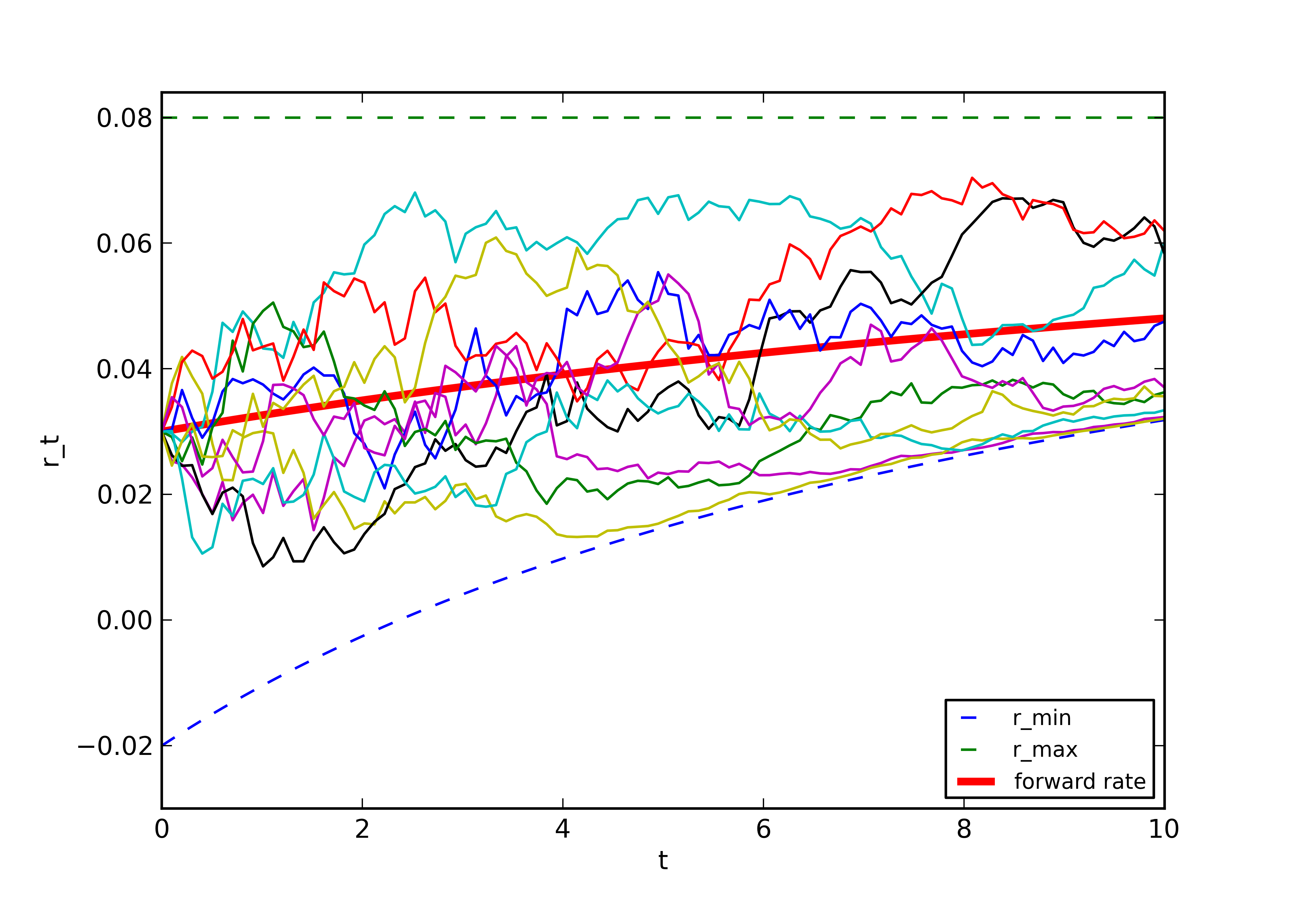
The resulting asymptotic extinction of volatility of the process $X_{t}$ as $t\rightarrow\infty$ appears to be a theoretical limitation of a one-factor LGP framework. This behavior is illustrated in Fig. 2 where we show a few paths of a simulated short rate process. As will be shown in the next section, a two-factor formulation allows one to build dynamics where stochasticity does not die off as $t\rightarrow\infty$. Another limitation of the one-factor formulation is that it is only able to produce monotonic (increasing or decreasing) yield curves. In order to get a humped-shaped yield curve, one needs at least a two factor specification.

On the practical side, the effect of decaying stochasticity of $X_{t}$ in the one-factor formulation can be somewhat mitigated by a suitable choice of parameters. In particular, if the yield curve is not too steep, by taking $\bar{\mu}>\mu$, we can admit some negative short rates in the short term while guaranteeing that $r_{t}$ stays positive for longer maturities, as shown in Fig. 2 where $r_{t}$ can go negative for $t\leq 2$ years. Such simple trick allows one to somewhat delay shrinkage of the support region of $r_{t}$ for larger time horizons. Therefore, we expect that the one-factor version of the model can still be used for monotonic yield curves with sufficiently short time horizons.

Figure 2: Simulated paths of the short rate $r_{t}$ as a function of calendar time $t$ (in years) for the one-factor LGP process Eq.(19), for the following choice of parameters: $a=0.085$, $\mu=0.080$, $\bar{\mu}=0.081$, $Y_{0}=0.909$ and $\hat{\sigma}=0.6$.

3.3 Extension to a Multi-Factor Case

The previous formulation treats a one-factor case $N=1$. For an arbitrary number of factors $N\geq 1$, the state vector ${\bf X}_{t}=\left(X_{1t},\ldots,X_{Nt}\right)$ satisfies the following equation:

$$d{\bf X}_{t}=r_{t}{\bf X}_{t}dt+\boldsymbol{\sigma}(t,{\bf X}_{t})\left[\boldsymbol{\lambda}(t,{\bf X}_{t})dt+d{\bf W}_{t}\right],$$ (27)

where ${\bf W}_{t}$ is a $N$-dimensional standard Brownian motion and the short rate $r_{t}$ is an affine function of ${\bf X}_{t}$:

$$r_{t}=a-c\sum_{i=1}^{N}e^{-\mu_{i}t}X_{it}\equiv a-c\sum_{i=1}^{N}\tilde{X}_{it}$$ (28)

where $\tilde{X}_{it}=e^{-\mu_{i}t}X_{it}$ are detrended state variables with $\mu_{i}$ being the corresponding growth rates, and $a>0$ and $c>0$ are non-negative constants. The $\mathbb{P}$-measure SDE for the state price deflator $M_{t}$ reads

$$\frac{dM_{t}}{M_{t}}=-r_{t}dt-\boldsymbol{\lambda}(t,X_{t})d{\bf W}_{t}$$ (29)

The solution to this equation generalizes Eq.(23):

$$M_{t}=\frac{\sum_{i=1}^{N}e^{-\mu_{i}t}\left[\alpha_{i}\kappa_{i}(t)+\beta_{i}Z_{t}\right]}{\sum_{i=1}^{N}(\alpha_{i}+\beta_{i})}$$ (30)

where parameters $\alpha_{i},\beta_{i}$ and functions $\kappa_{i}(t)$ with $i=1,\ldots,N$ are defined similarly to Eq.(20). Finally, the solution for the bond price in a $N$-factor model generalizes Eq.(9) (Bekker & Bouwman, (2009)):

$$P(t,T)=e^{-a\tau}\left[1+c\sum_{i=1}^{N}e^{-\mu_{i}t}\frac{e^{(a-\mu_{i})\tau}-1}{a-\mu_{i}}X_{it}\right]=e^{-a\tau}\left[1+c\sum_{i=1}^{N}\frac{e^{(a-\mu_{i})\tau}-1}{a-\mu_{i}}\tilde{X}_{it}\right]$$ (31)

where $\tau=T-t$. As can be seen from Eq.(31), only the factor with the smallest value of $\mu$ contributes to this expression in the limit $T\rightarrow\infty$. In our analysis below we set $N=2$ and assume that $\mu_{2}<\mu_{1}$. Therefore, we interpret the second factor $X_{2t}$ as a long term factor, while $X_{1t}$ serves as a short-term factor that drives, jointly with $X_{2t}$, the short-term part of the yield curve. A two-factor specification gives rise to a richer set of yield curves than a one-factor one, including, in particular, humped curves or curves with sign-changing convexity which could not be obtained with a one-factor specification.

Another key difference of a multi-factor case from a one-factor one is that volatility does not necessarily die off in the long run. We can illustrate this for $N=2$. Proceeding similarly to the one-factor case, we first solve the system Eq.(27) without noise, by setting $\boldsymbol{\sigma}(t,{\bf X}_{t})=0$. We obtain

$$\tilde{X}_{1t} = \frac{a-\mu_{1}}{c}\frac{e^{-(\mu_{1}-a)t}}{\xi_{0}-\eta_{0}e^{-(\mu_{2}-a)t}+e^{-(\mu_{1}-a)t}}$$

$$\tilde{X}_{2t} = \eta_{0}\frac{\mu_{2}-a}{c}\frac{e^{-(\mu_{2}-a)t}}{\xi_{0}-\eta_{0}e^{-(\mu_{2}-a)t}+e^{-(\mu_{1}-a)t}}$$ (32)

where $\eta_{0}$ and $\xi_{0}$ are two constants that are determined by initial conditions. In what follows, we assume that $\mu_{1}>a$ and $a<\mu_{2}<\mu_{1}$, as suggested by a numerical example below. For such a scenario, the following constraints on parameters $\eta_{0}$ and $\xi_{0}$:

$$0\leq\eta_{0}\leq 1\,,\;\;\xi_{0}\geq 1$$ (33)

guarantee that Eq.(3.3) is well defined at all times. Additional constraints on parameters $\eta_{0}$ and $\xi_{0}$ arise if we enforce positivity of the short rate $r_{t}=a-c\tilde{X}_{1t}-c\tilde{X}_{2t}$. We will omit details that can be reproduced using similar steps to the above one-factor case, and instead concentrate on showing that volatility in a two-factor (or, more generally, a multi-factor) LGP-type model does not in general die off in the long term.

To this end, we note that a solution of a full $N=2$ model with non-vanishing volatility $\boldsymbol{\sigma}(t,{\bf X}_{t})\neq 0$ can be obtained along similar lines to the previous $N=1$ case. More specifically, we should replace constants $\xi_{0}$ and $\eta_{0}$ in the deterministic solution Eq.(3.3) by judiciously chosen fractional-linear functions of a two-dimensional martingale process ${\bf Z}_{t}=\left(Z_{1t},Z_{2t}\right)$. The latter satisfies a two-factor generalization of Eq.(17), and has the initial value ${\bf Z}_{0}=(1,1)$. On the other hand, assuming that $\mu_{1}>a$ and $a<\mu_{2}<\mu_{1}$, the asymptotic behavior of the deterministic solution Eq.(3.3) as $t\rightarrow\infty$ is as follows:

$$\tilde{X}_{1t}\rightarrow\frac{a-\mu_{1}}{c}\frac{1}{\xi_{0}}e^{-(\mu_{1}-a)t}\;,\;\;\tilde{X}_{2t}\rightarrow\frac{\mu_{2}-a}{c}\frac{\eta_{0}}{\xi_{0}}e^{-(\mu_{2}-a)t}$$ (34)

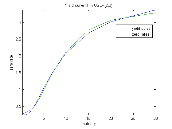
This suggests that volatility of factors $X_{1t}\,X_{2t}$ does not necessarily get extinct in the long run, unlike the behavior observed in the one-factor case. An example of a calibrated yield curve is shown in Fig. 3.

Figure 3: Calibrated yield curve (as a function of maturity in years) on 03/15/13 in the two factor model. Calibrated parameters are as follows: $a=0.041,\,\mu_{1}=0.520,\,\mu_{2}=0.382,\,X_{1}=-0.151,\,X_{2}=0.188$.

4 The USLV Model

Until this point, our formalism has largely followed the CGW model by Carr et al., (2011) (albeit using the formulation of LGP dynamics proposed by Bekker & Bouwman, (2009)). Now it is time to part ways.

CGW investigate a parametric stochastic volatility (SV) specification of the dynamics of $Z_{t}$. In that specification, the stock volatility is obtained by a stochastic time change with an activity rate process given by a superposition of CIR processes.

Our plan is different. We want to stick to simple one- or two-factor specifications of the stochastic volatility process, while concentrating on modeling a nonparametric local volatility layer in Eq.(17) in such a way that all observable option quotes would be exactly matched. Furthermore, our approach is necessarily numerical and is based on a Markov chain approximation to the dynamics of the martingale $Z_{t}$.

We will construct our model in two steps. In the first step, we develop a discretized nonparametric local volatility version of USLV that corresponds to a zero vol-of-vol limit of the full-blown model. Calibration to option quotes in this framework is achieved via a set of multiplicative adjustment factors acting on elements of the Markov generator (see below). We will refer to these adjustment factors as the one-dimensional (1D) Speed Factors (SFs). Calibration of such a one-dimensional USLV model amounts to computing a set of 1D SFs.

In the second step, we move on to a full-blown USLV model with a nonzero vol-of-vol by turning stochastic volatility on. In the present discrete-space framework, this amounts to making the Markov chain generator stochastic.

To retain a near-perfect calibration to a set of option quotes obtained in the first (1D) step, we introduce another set of speed factors which we will refer to as 2D speed factors (2D SFs). The 2D SFs are then calibrated from the previously computed 1D SFs using a version of the Markovian projection method implemented in an efficient manner using forward induction on the Markov chain. Once calibrated, the resulting 2D Markov chain can be utilized to set up efficient pricing schemes for derivatives based on backward-induction algorithms.

We note that the resulting discrete-space continuous-time dynamics on a Markov chain with a stochastic generator arising in our approach resembles the BSLP model developed for portfolio credit derivatives in Arnsdorf & Halperin, (2007). The two models are similar in that both use a two-step approach to calibration. In addition, both the definition and parametrization of our speed factors are similar to how analogously defined contagion factors are introduced and used in the BSLP model. The difference of the USLV model from the BSLP model is that while a discrete-space description is exact for credit, it is used as an approximation to the dynamics of the underlying for USLV. Furthermore, while the BSLP model uses a non-linear death process as a model for a portfolio loss, in the present case we use a nonlinear quasi-birth-death (QBD) process as a discrete approximation to the dynamics of a two-dimensional Markov driver ${\bf Z_{t}}=\left(Z_{t}^{(1)},Z_{t}^{(2)}\right)^{\top}$. Finally, we use a different method for an efficient computation of matrix exponentials arising in evaluation probabilities on Markov chains.

In what follows, we use the following compact notation for different flavors of our model. We denote one- and two-factor discretized local volatility models as USLV(1,0) and USLV(2,0), respectively. Versions with stochastic volatility are denoted as USLV(1,1), (2,1), or (2,2). We call a discretized process for ${\bf Z_{t}}=\left(Z_{t}^{(1)},Z_{t}^{(2)}\right)^{\top}$ a 1D process, while the joint process of ${\bf Z_{t}}$ and stochastic volatility is referred to as a 2D process.

4.1 USLV(1,0): One-Factor Local Volatility

We consider the following SDE describing a local volatility dynamics of a one-dimensional Markov driver $Z_{t}$ under the $\mathbb{P}$-measure:

$$\frac{dZ_{t}}{Z_{t}}=\hat{\sigma}(Z_{t},t)dW_{t},$$ (35)

where $W_{t}$ is a Brownian motion and $\hat{\sigma}(Z_{t},t)$ is a local volatility. Our objective is to discretize the dynamics corresponding to Eq.(35).

To this end, we first construct a nonuniform grid of possible values of the martingale $Z_{t}>0$ with $Z_{0}=1$. Let $p$ be the number of points on the grid and $0<z_{0}<z_{1}<\cdots<z_{p-1}$ be the nodes on the grid. Irregularity of the grid allows making it denser in interesting regions, and sparser in uninteresting ones. Clearly, the fact that our process is a martingale helps as our grid should not be too large: as time passes, the underlying stays around the current value in the sense of expectations.

Let the current state be $z_{i}$ and let $\Delta z_{i,i-1}=z_{i}-z_{i-1},\ i\in[1,p-1]$ be the $i$th space interval on the grid. We construct the elements of the generator matrix $A_{t}$ following the adaptive Markov chain approximation of Cerrato et al., (2011). Adapting their formulae to our case of a zero-drift diffusion $Z_{t}$, we obtain the Markov chain generator

$$A\,=\,\left(\begin{array}[]{ccccc}a_{00}&a_{01}&0&\cdots&0\\ a_{10}&a_{11}&a_{12}&\cdots&0\\ \vdots\\ 0&\cdots&a_{p-2,p-3}&a_{p-2,p-2}&a_{p-2,p-1}\\ 0&\cdots&0&a_{p-1,p-2}&a_{p-1,p-1}\end{array}\right)$$ (41)

with elements

$$a_{i,i-1} =\frac{s_{i}(t)}{\Delta z_{i,i-1}\left(\Delta z_{i,i-1}+\Delta z_{i+1,i}\right)},\quad a_{i,i+1}=\frac{s_{i}(t)}{\Delta z_{i+1,i}\left(\Delta z_{i,i-1}+\Delta z_{i+1,i}\right)},$$ (42)

$$a_{ii} =-a_{i,i-1}-a_{i,i+1},\quad a_{i+j,i}=a_{i,i+j}=0,\qquad j>1.$$

where we defined a grid-valued set of speed factors (SFs)

$$s_{i}(t)=\hat{\sigma}^{2}(z_{i},t).$$ (43)

Now we have a Markov generator parametrized by the pointwise set of speed factors in Eq.(43). Next we will show how the SFs in Eq.(43) are turned into tunable parameters and used for calibration to option quotes.

4.2 Parametrization of Speed Factors in USLV(1,0)

As it stands, the parametrization in Eq.(41) is very general. The number of free parameters per a given time slice $t$ is $p$, typically far exceeding the number of observed option quotes available for calibration for cases of practical interest.

To achieve an exact match between the number of free parameters in our model and the number of available option quotes, we consider the following parametrization of our 1D speed factors Eq.(43). Our approach here is similar to how contagion factors are used in the BSLP model of Arnsdorf & Halperin, (2007).

We assume that as a function of time $t$, the SFs $s_{i}(t)$ are piecewise constant between maturities of traded options. This considerably simplifies computation of matrix exponentials.

For the dependence of $s_{i}(t)$ on the grid index $i$ (i.e., for the $z$ dependence), we proceed as follows. Let $K_{0},K_{1},\ldots,K_{q-1}$ be a set of strikes for traded options across all maturities, expressed in terms of the $Z$-space as, e.g., in Proposition 3 of Carr et al., (2011). We assume that all these strikes correspond to $q$ different nodes on our grid. We then model the speed factors $s_{i}$ for all values of $i$ by picking exactly $q$ free values $\hat{s}_{0},\ldots,\hat{s}_{q-1}$ at locations $K_{0},K_{1},\ldots,K_{q-1}$, and using linear interpolation for points in between. In other words, our speed factors $s_{i}(t)$ are piecewise-linear in $z_{i}$, while the anchor points at $q$ selected nodes serve as free parameters for calibration to option quotes. Any consistent set of option quotes can be exactly matched by the present method.

Note that calibration of local volatility models without assuming availability of a complete set of option quotes (i.e., when the number of option quotes is less then the number of nodes on a grid) has been previously discussed in the literature. In particular, a recent paper by Lipton & Sepp, (2011) analyzes a setting where the local volatility function is piecewise-flat between quoted strikes (or between mid-points) using Laplace-transform based methods. Unlike their method, which is exact in 1D, our approach is based on numerical optimization, but it is extendable to a multivariate setting (2D and higher) along the same lines as in 1D. In addition, a piecewise-linear volatility model appears to be a less drastic approximation than a piecewise-flat model.

4.3 Calibration of the USLV(1,0) Model

Calibration of the speed factors $s_{i}(t)$ in the above setting is straightforward. The anchor points introduced above serve as parameters of optimization. Given a multidimensional optimizer, at each iteration we first construct the generator matrix given the current set of the anchor points. After that, finite-time probability distributions are computed by taking matrix exponentials of the generator. As the mathematical structure of our model is essentially the same for the $N=1$ and $N=2$ cases (one or two factors for the term structure), we postpone presenting details of this procedure until the next section where we introduce an $N=2$ version of our model. Theoretical option prices for a given set of model parameters are then computed using these probability distributions. Finally the optimizer adjusts the current set of free parameters to decrease the error between the model and the market.

5 USLV(2,0): Two Curve Factors

With two factors for the curve ($N=2$), we assume the following vector-valued SDE for the dynamics of ${\bf Z}_{t}=\left(Z_{t}^{1},Z_{t}^{2}\right)^{\top}$:

$$\left(\begin{array}[]{cc}dZ_{t}^{(1)}\\ dZ_{t}^{(2)}\\ \end{array}\right)=\left(\begin{array}[]{cc}\Sigma_{11}&\Sigma_{12}\\ \Sigma_{21}&\Sigma_{22}\\ \end{array}\right)\left(\begin{array}[]{cc}dW_{t}^{(1)}\\ dW_{t}^{(2)}\\ \end{array}\right),$$ (50)

where two Brownian motions $W_{t}^{(1)},W_{t}^{(2)}$ are independent, and the volatility matrix $\Sigma=\Sigma(\bf z)$ is defined as follows:

$$\Sigma({\bf z})=\sqrt{s({\bf z},t)}\left(\begin{array}[]{cc}\sigma_{1}\sqrt{1-\rho^{2}}&\sigma_{1}\rho\\ 0&\sigma_{2}\\ \end{array}\right),\;\;\;\Sigma({\bf z})\Sigma({\bf z})^{T}=s({\bf z},t)\left(\begin{array}[]{cc}\sigma_{1}^{2}&\rho\sigma_{1}\sigma_{2}\\ \rho\sigma_{1}\sigma_{2}&\sigma_{2}^{2}\\ \end{array}\right).$$ (55)

Here $s({\bf z},t)=s({\bf Z}_{t},t|{\bf Z}_{t}={\bf z})\geq 0$ is a scalar function of the state variable ${\bf Z}_{t}=\left(Z_{t}^{(1)},Z_{t}^{(2)}\right)^{\top}$, and ${\bf z}=(z_{1},z_{2})$ are the values of ${\bf Z}_{t}$ at time $t$. An explicit specification of this function will be given below. Note that components $Z_{t}^{(1)}$ and $Z_{t}^{(2)}$ defined by Eq.(50) and Eq.(55) are correlated with correlation coefficient $\rho$.

Our first objective is to approximate the dynamics given by Eq.(50) by a 2D Markov chain. To this end, we start with a Markov generator corresponding to the 2D diffusion given by Eq.(50):

$$\mathcal{L}V({\bf z})=\frac{1}{2}\sum_{i,j=1}^{N=2}\left[\Sigma\Sigma^{T}\right]_{ij}\frac{\partial^{2}V(\bf z)}{\partial z_{i}\partial z_{j}},$$ (56)

where $V({\bf z})=V({\bf z}_{T}|{\bf z})$ is an arbitrary function (a value function or a transition density) of backward variables ${\bf z}$ (with forward variables ${\bf z}_{T}$ treated as parameters). The generator specifies the continuous-space backward equation

$$\frac{\partial V\left({\bf z},t\right)}{\partial t}=-\mathcal{L}V\left({\bf z},t\right).$$

Note that in order to be probabilistically interpretable as a generator of a Markov chain, a discrete version $A$ of the generator $\mathcal{L}$ should have all nondiagonal elements nonnegative, and all diagonal elements negative, such that all rows sum up to one. These remarks are important as not any discretization of $\mathcal{L}$ gives rise to a valid Markov chain generator. For example, using a central divided difference to approximate the mixed derivatives in Eq.(56) would not preserve nonnegativity of nondiagonal elements of $A$.

With these remarks in mind, and given a two-dimensional grid of values of $\left(Z^{(1)},Z^{(2)}\right)$ with $p$ nodes per dimension, we approximate second derivatives by divided differences. Derivatives $V_{z_{k},z_{k}},\ k=1,2$, are represented using the central differences

$$\left.\frac{\partial^{2}V}{\partial z_{1}^{2}}\right|_{ij} =\frac{V_{i+1,j}-2V_{i,j}+V_{i-1,j}}{(\Delta z_{1})^{2}}+O\left((\Delta z_{1})^{2}\right),$$

$$\left.\frac{\partial^{2}V}{\partial z_{2}^{2}}\right|_{ij} =\frac{V_{i,j+1}-2V_{i,j}+V_{i,j-1}}{(\Delta z_{2})^{2}}+O\left((\Delta z_{2})^{2}\right),$$

while for the mixed derivative we take uncentered differences which preserve nonnegativity:

$$\left.\frac{\partial^{2}V}{\partial z_{1}\partial z_{2}}\right|_{ij} =\frac{V_{i+1,j+1}-V_{i+1,j}-(V_{i,j+1}-2V_{ij}+V_{i,j-1})-(V_{i-1,j}-V_{i-1,j-1})}{2\Delta z_{1}\Delta z_{2}}$$

$$+O\left(\Delta z_{1}\Delta z_{2}\right)+O\left((\Delta z_{1})^{2}\right)+O\left((\Delta z_{2})^{2}\right),\quad\rho\geq 0,$$

$$\left.\frac{\partial^{2}V}{\partial z_{1}\partial z_{2}}\right|_{ij} =\frac{V_{i+1,j}-V_{i+1,j-1}+(V_{i,j+1}-2V_{ij}+V_{i,j-1})-(V_{i-1,j+1}-V_{i-1,j})}{2\Delta z_{1}\Delta z_{2}}$$

$$+O\left(\Delta z_{1}\Delta z_{2}\right)+O\left((\Delta z_{1})^{2}\right)+O\left((\Delta z_{2})^{2}\right),\quad\rho<0.$$

Using this in Eq.(56) and regrouping terms, we obtain

$$\left(\mathcal{L}V(z)\right)_{ij}=\sum_{k,m\in\{-1,0,1\}}a_{ij|i+k,j+m},V_{i+k,j+m}$$ (57)

where we introduced the following compact notation:

$$a_{ij|i+1,j} =a_{ij|i-1,j}=\frac{1}{2}s_{ij}(t)\left(\frac{\sigma_{1}^{2}}{\left(\Delta z_{1}\right)^{2}}-\frac{|\rho|\sigma_{1}\sigma_{2}}{\Delta z_{1}\Delta z_{2}}\right),$$

$$a_{ij|i,j+1} =a_{ij|i,j-1}=\frac{1}{2}s_{ij}(t)\left(\frac{\sigma_{2}^{2}}{\left(\Delta z_{2}\right)^{2}}-\frac{|\rho|\sigma_{1}\sigma_{2}}{\Delta z_{1}\Delta z_{2}}\right),$$

$$a_{ij|ij} =-s_{ij}(t)\left(\frac{\sigma_{1}^{2}}{\left(\Delta z_{1}\right)^{2}}-\frac{|\rho|\sigma_{1}\sigma_{2}}{\Delta z_{1}\Delta z_{2}}+\frac{\sigma_{2}^{2}}{\left(\Delta z_{2}\right)^{2}}\right),$$ (58)

$$a_{ij|i+1,j+1} =a_{ij|i-1,j-1}=\left\{\begin{array}[]{ll}\frac{s_{ij}(t)}{2}\frac{\rho\sigma_{1}\sigma_{2}}{\Delta z_{1}\Delta z_{2}}&\mbox{if $\rho\geq 0$},\\ 0&\mbox{if $\rho<0$},\end{array}\right.$$ (61)

$$a_{ij|i+1,j-1} =a_{ij|i-1,j+1}=\left\{\begin{array}[]{ll}0&\mbox{if $\rho\geq 0$},\\ \frac{s_{ij}(t)}{2}\frac{|\rho|\sigma_{1}\sigma_{2}}{\Delta z_{1}\Delta z_{2}}&\mbox{if $\rho<0$},\end{array}\right.$$ (64)

where $s_{ij}(t)=\left[s(Z_{t},t)\right]_{ij}$.

To ensure that all parameters $a_{ij|i+k,j+m},\ k,m\neq 0$ are nonnegative, we impose the following constraint on the step size $\Delta z_{2}$ given a chosen step $\Delta z_{1}$:

$$|\rho|\frac{\sigma_{2}}{\sigma_{1}}\Delta z_{1}\leq\Delta z_{2}\leq\frac{\sigma_{2}}{|\rho|\sigma_{1}}\Delta z_{1}.$$ (65)

Assuming Eq.(65) is satisfied, we can interpret Eq.(57) as a generator matrix of a 2D Markov chain. We can write it in a matrix form as follows:

$$\left(\mathcal{L}V(z)\right)_{ij}=\left[AV\right]_{ij}=\sum_{i^{\prime},j^{\prime}}A_{ij|i^{\prime}j^{\prime}}V_{i^{\prime}j^{\prime}}.$$ (66)

As we deal with a two-factor setting, the matrix elements of the generator $A$ carry four indices rather than two. To sum over two indices corresponding to the $Z^{(1)}$- and $Z^{(2)}$-states in Eq.(66), it is convenient to group all transitions according to the change of one variable (e.g., $Z^{(1)}$). We obtain

$$\left(\mathcal{L}V(z)\right)_{ij}=\sum_{i^{\prime},j^{\prime}}A_{ij|i^{\prime}j^{\prime}}V_{i^{\prime}j^{\prime}}=\sum_{j^{\prime}}A_{ij|i-1,j^{\prime}}V_{i-1,j^{\prime}}+\sum_{j^{\prime}}A_{ij|ij^{\prime}}V_{ij^{\prime}}+\sum_{j^{\prime}}A_{ij|i+1,j^{\prime}}V_{i+1,j^{\prime}}$$

$$=\left[\left\{a_{ij|i-1,j-1}V_{i-1,j-1}+a_{ij|i-1,j}V_{i-1,j}+a_{ij|i-1,j+1}V_{i-1,j+1}\right\}\right.$$

$$\qquad\left.+\left\{a_{ij|i,j-1}V_{i,j-1}+a_{ij|ij}V_{ij}+a_{ij|i,j+1}V_{i,j+1}\right\}\right.$$ (67)

$$\qquad\left.+\left\{a_{ij|i+1,j-1}V_{i+1,j-1}+a_{ij|i+1,j}V_{i+1,j}+a_{ij|i+1,j+1}V_{i+1,j+1}\right\}\right].$$

Here terms in the first, second, and third row correspond to transitions $i\rightarrow i-1$, $i\rightarrow i$, and $i\rightarrow i+1$ in the $Z^{(1)}$-dimension, respectively.

Mathematically, this is expressed via the following tridiagonal block-matrix form for the resulting “one-dimensional” Markov chain generator $A$:

$$A\,=\,\left(\begin{array}[]{clcrccc}L^{(0)}&F^{(0)}&0&0&\cdots&0&0\\ B^{(1)}&L^{(1)}&F^{(1)}&0&\cdots&0&0\\ 0&B^{(2)}&L^{(2)}&F^{(2)}&\cdots&0&0\\ \vdots\\ 0&0&0&0&\cdots&B^{(p-1)}&L^{(p-1)}\\ \end{array}\right),$$ (73)

where all matrices $B^{(i)},L^{(i)},\,F^{(i)}$ have dimension $p\times p$, i.e., the dimension of our one-dimensional grids. Explicit expressions for these matrices can be found from Eq.(5):

$$B_{j,j-1}^{(i)}=a_{ij|i-1,j-1},\;B_{j,j}^{(i)}=a_{ij|i-1,j},\;B_{j,j+1}^{(i)}=a_{ij|i-1,j+1},$$

$$L_{j,j-1}^{(i)}=a_{ij|i,j-1},\;L_{j,j}^{(i)}=a_{ij|ij},\;L_{j,j+1}^{(i)}=a_{ij|i,j+1,},$$ (74)

$$F_{j,j-1}^{(i)}=a_{ij|i+1,j-1},\;F_{j,j}^{(i)}=a_{ij|i+1,j},\;F_{j,j+1}^{(i)}=a_{ij|i+1,j+1},$$

while all other elements of these matrices vanish. Note that this implies that the generator Eq.(73) is “doubly” sparse, as matrices $B^{(i)},L^{(i)}$ and $F^{(i)}$ are themselves sparse; see also a comment at the end of this section.

The block-tridiagonal matrix structure Eq.(73) of the Markov chain generator $A$ is characteristic of so-called quasi-birth-death (QBD) processes. A QBD process is a bivariate Markov chain of a special type of dynamics of two components. The first component, $Z_{t}^{(1)}$, called the “level,” follows a birth-and-death (BD) process on either a finite or infinite set of states. Conditional on the realization of the $Z_{t}^{(1)}$-component at a given step $[t,t+dt]$, the second component $Z_{t}^{(2)}$, called the “phase,” follows another Markov process. For a short review of QBD processes, see, e.g., Kharoufeh, (2011). Note that in our particular case, $Z_{t}^{(2)}$ follows another BD process, while the support of $Z_{t}^{(1)}$ is finite. QBD processes with finite support are called finite QBD processes.

The symbols $L,B$ and $F$ in Eq.(73) stand for local (without change of level), backward and forward (the level is changed by one unit up or down) moves, respectively. Note that as long as the matrices $L^{(i)},B^{(i)}$ and $F^{(i)}$ depend on level $i$ via the discretized local volatility function $s_{ij}$, our QBD process with generator Eq.(73) is a level-dependent (or nonlinear) finite QBD, denoted sometimes as a (finite) LDQBD in the literature.

It is easy to check that Eq.(73) with elements defined as in Eq.(5) is a valid Markov generator where all off-diagonal elements are positive, diagonal elements are negative and each row in $A$ sums to zero.

After the QBD generator matrix is constructed according to Eq.(73), a matrix $P$ of finite-time transition probabilities with matrix elements

$$P_{ij|i^{\prime}j^{\prime}}(t,T)\equiv P\left[(Z_{T}^{(1)},Z_{T}^{(2)}=z_{i^{\prime}}^{(1)},z_{j^{\prime}}^{(2)}|Z_{t}^{(1)},Z_{t}^{(2)}=z_{i}^{(1)},z_{j}^{(2)}\right]$$ (75)

can be computed by solving the forward Kolmogorov equation

$$\frac{\partial P}{\partial T}=PA.$$ (76)

For a given interval $[t_{1},t_{2}]$ where the generator $A$ does not depend on time, the solution of the forward equation is

$$P=P_{t_{1}}e^{(t_{2}-t_{1})A},$$

where $P_{t_{1}}$ is a state vector at time $t_{1}$, and $e^{X}$ stands for the matrix exponential of $X$.

A few remarks on the complexity of the method just presented are in order here. We have managed to map the two-factor continuous-space dynamics Eq.(50) on the state space $Z_{1}\times Z_{2}$ onto a QBD process with generator Eq.(73). The latter can formally be viewed as a one-dimensional Markov chain in an extended linear space whose basis is formed by elements of a Kroneker product of grid values ${\bf Z}_{g}^{(1)}\otimes{\bf Z}_{g}^{(2)}$ (and properly rearranged to form a QBD structure). Therefore, computation of transition probabilities Eq.(76) in our two-factor model is, at least formally, as simple as a corresponding calculation for a one-factor model, and reduces to computation of a single matrix exponential, albeit of a larger matrix.

While naively the generator $A$ has $O(p^{4})$ free parameters, their actual number is much lower due to sparsity of the matrix. It is simple to find that the number of nonzero elements that need to be stored scales as $(3p-2)p+2(2p-1)^{2}$. For example, for $p=100$ our matrix $A$ would be of size $10000\times 10000$ with only 109,002 non-zero elements. Matrices of such sizes can well be handled by modern matrix exponentiation methods (see below).

5.1 Transient Probabilities of QBD Chain by Randomization

It is well known that a direct computation of a matrix exponential $e^{tA}$ with a Markov generator $A$ via a straightforward use of a Taylor series expansion as $\sum_{n=0}^{\infty}(tA)^{n}/n!$ is in general not a good idea (see Moler & van Loan, (2003)). The main reason for this is that severe roundoff errors might accumulate (especially when the matrix is large) due to the fact that the generator has both positive and negative entries. In addition, matrices $(tA)^{n}$ become nonsparse even if the original matrix $A$ is sparse, as is the case for the QBD process.

An efficient method of choice for dealing with matrix exponentials for large matrices is known as Jensen’s randomization; see, e.g., Gross & Miller, (1984), or Haverkort, (2001) for a more recent review. The method proceeds as follows. We start with choosing a parameter $\lambda\geq\max_{i}\left\{|A_{ii}|\right\}$, and define the matrix

$${\bf P}={\bf I}+\frac{{\bf A}}{\lambda}\;\Rightarrow{\bf A}=\lambda\left({\bf P}-{\bf I}\right).$$ (77)

With our choice of $\lambda$, all entries of ${\bf P}$ are between 0 and 1, and all rows sum to 1. This means that ${\bf P}$ is a stochastic matrix that describes a discrete-time Markov chain “related” to the original continuous-time Markov chain with generator $A$. We now want to discuss in more detail the sense in which these two Markov chains are “related.”

To this end, we substitute $A$ as given by Eq.(77) into the solution of the forward equation:

$$P(t)=P_{0}^{\prime}e^{tA}=P_{0}^{\prime}e^{\lambda t\left({\bf P}-{\bf I}\right)}=P_{0}^{\prime}e^{-\lambda t}e^{\lambda{\bf P}t}.$$

Using a Taylor series expansion for the matrix exponential in this expression, we obtain

$$P(t)=P_{0}^{\prime}e^{-\lambda t}\sum_{n=0}^{\infty}\frac{\left(\lambda t\right)^{n}{\bf P}^{n}}{n!}=P_{0}^{\prime}\sum_{n=0}^{\infty}\psi(\lambda t,n){\bf P}^{n},$$ (78)

where

$$\psi(\lambda t,n)=e^{-\lambda t}\frac{(\lambda t)^{n}}{n!},\;\;n\in\mathbb{N},$$

are Poisson probabilities, i.e., probabilities of observing $n$ events by time $t$ for a Poisson process with intensity $\lambda$. Note that a naive Taylor expansion of the matrix exponential $e^{tA}$ behaves badly, but the new expansion is much better behaved: roundoff errors are now largely eliminated as all entries of matrix ${\bf P}$ are between 0 and 1. Moreover, different terms are weighted by the Poisson probabilities, so that the expansion is expected to converge fast when the product $\lambda t$ is not too large.

We note that the construction given by Eq.(78) can be interpreted as a discrete-time Markov chain (DTMC) $Y_{n}$ ($n=0,1,\ldots,p$) with transition matrix ${\bf P}$ subordinated to a Poisson process $N_{t}$ where the latter serves as a randomized “operational time” for $Y_{n}$, so that the subordinated process is now defined as $X_{t}=Y_{N_{t}}$ (see, e.g., Feller, (1968)). We will return to the topic of subordinated processes in Sect. 7.1.

It is important to point out that the method just presented can be used without a matrix-matrix multiplication (as Eq.(78) would naively suggest). Let ${\hat{\bf\pi}}_{n}$ be the probability distribution vector in the DTMC with transition matrix ${\bf P}$ after $n$ epochs. This vector can be computed recursively:

$${\hat{\bf\pi}}_{0}={\bf P}_{0},$$

$${\hat{\bf\pi}}_{n}={\hat{\bf\pi}}_{n-1}{\bf P},\;\;n\in{\mathbb{N}}^{+}.$$ (79)

Using the vector ${\hat{\bf\pi}}_{n}$, the state probabilities Eq.(78) in the original CTMC are computed as follows:

$$P(t)=\sum_{n=0}^{\infty}\psi(\lambda t,n)\left(P_{0}^{\prime}{\bf P}^{n}\right)=\sum_{n=0}^{\infty}\psi(\lambda t,n){\hat{\bf\pi}}_{n}.$$

Therefore, computationally the algorithm amounts to a series of vector-matrix multiplications that can be done very efficiently for matrices of sizes typical for our problem. Moreover, the recursive procedure of Eq.(5.1) preserves the sparsity of ${\bf P}$, thus enabling a substantial acceleration of the vector-matrix multiplication.

In practice, the infinite sum in Eq.(78) is truncated at some value $n_{max}$. This value can be adaptively controlled within the algorithm itself, as a theoretical upper bound for an error resulting from the truncation is available as discussed, e.g., by Gross and Miller (1984).

5.2 Calibration of Speed Factors in USLV(2,0)

Summarizing our results for the USLV(2,0) model so far, we see that the mathematical structure of the (2,0) model is similar to that of the (1,0) model. Indeed, for the latter our Markov chain construction gives rise to a nonlinear birth-death (BD) process modulated by 1D speed factors (SFs) $s_{i}(t)$. After a proper parametrization as described in Sect. 4.2, SFs are calibrated to market option quotes. For the (2,0) case (two factors for the term structure), the resulting Markov chain is a nonlinear quasi-birth-death process, again modulated by a set of SFs $s_{ij}$. In terms of computational complexity, the two cases are essentially the same, as both amount to calculation of matrix exponentials of a Markov chain generator (albeit in different dimensions).

Calibration of the (2,0) model is done by the fitting function $s(z,t)$ in Eq.(50). To this end, we proceed similarly to the one-factor case. We assume that function $s(z,t)=s(z_{1},z_{2},t)$ is a function of single argument, $s(z_{1},z_{2},t)=s(\alpha_{1}z_{1}+\alpha_{2}z_{2},t)$, where $\alpha_{1},\alpha_{2}\geq 0$ are some weights (e.g., $\alpha_{1}=\alpha_{2}=0.5$). For calibration purposes, we could parametrize this function in a piecewise-linear way, i.e., in exactly the same way as we did before for the $N=1$ model. The number of free parameters (anchor points) and their locations would be chosen based on a particular set of instruments available for calibration.

To continue with our theoretical construction of the model, in what follows we assume that the stage of construction of a (2,0) (or (1,0)) version of the USLV model is completed along the lines described here. In what follows, we refer to these SFs as 1D SFs, in order to differentiate them from another set of speed factors (2D SFs) that will be introduced below when we add stochastic volatility to the model.

Finally, we note that while the main purpose of the USLV(2,0) model for our purposes is to use it as a building block in the construction of a full-blown USLV(2,2) model with stochastic volatility, the pure local volatility USLV(2,0) model can also be useful in its own right, e.g., as a way of pricing European vanilla options with illiquid strikes in terms of prices of liquidly traded options.

6 USLV(2,2): Two Curves and Two Volatility Factors

Once we have a calibrated USLV(2,0) model, introduction of stochastic volatility in this framework amounts to two things: (i) introducing new dynamics for volatility drivers, and (ii) making sure the model still calibrates to available option prices. This produces a calibrated USLV(2,2) model.

Let us note that stochastic volatility dynamics can be introduced in our framework in two ways. In the first approach, we follow the formulation of a continuous-time Markov chain (CTMC) dynamics, which we now augment by 2D dynamics of “spot” variance factors. For numerical implementation, the model is then put on a time grid $[t_{0},t_{1},\ldots,t_{n}]$ with a uniform time step $\Delta t$. All calculations (see below) are done to $O(\Delta t^{2})$ accuracy, which assumes that $\Delta t$ should be sufficiently small. With this method, we solve the forward and backward Kolmogorov equations one step $\Delta t$ at a time, similarly to finite difference methods.

In the second approach, we deal with arbitrary time lines which do not necessarily have small time steps. For example, we may want to model the values of underlying factors only on a sparse set of “interesting” dates (e.g., coupon dates, call dates etc.). Essentially, by taking matrix exponentials of the generator, we aim here to achieve a functionality similar to the USLV(1,0) and USLV(2,0) models (or any CTMC model, for that matter), which are capable of computing finite-time transition probabilities directly.

Respectively, in what follows we present two versions of the USLV(2,2) model. In the first version, we assume a Markov dynamics in the pair $\left({\bf Z}_{t},{\bf Y}_{t}\right)$ where ${\bf Y}_{t}=\left(Y_{t}^{(1)},Y_{t}^{(2)}\right)$ is a bivariate “spot” variance driver. In the second version, we instead assume a Markov dynamics in a pair of ${\bf Z}_{t}$ and an integrated bivariate variance, or, more generally, a bivariate stochastic time subordinator (see below). We will use the notation ${\bf T}_{t}=\left(T_{t}^{(1)},T_{t}^{(2)}\right)$ for the latter in what follows. For reasons that will become clear shortly, we will refer to these two versions of the model as the activity-rate-based model (AR-USLV), or the implied-time-change-based model (ITC-USLV), respectively.

On the theoretical side, it turns out that both approaches can be viewed in a unified way by interpreting them as particular realizations of a stochastic time change of the original QBD Markov chain. We will give more details on this below in Sect. 7.1.

On the practical side, we can choose between two numerical methods. With the first method, we can implement both the AR- and ITC-versions of our model in a similar way using a version of the Markovian projection method. The latter reduces calibration of USLV(2,2) to a fast forward induction method in what is essentially a 1D problem, without a need for a forward induction on a full 2D Markov chain. No new optimization in addition to one performed at the stage of calibration of the USLV(2,0) model is involved here. Therefore, the method is very fast on each given time step, the only potential bottleneck being the necessity to perform such computation repeatedly on a dense time grid. The method is nonparametric in that it solves the problem of calibration of the full-blown USLV(2,2) model via a judicious choice of 2D speed factors (SFs) that are computed off the calibrated 1D SFs of the USLV(2,0) model.

The second method, which is applied below for the ITC-USLV version of our model but in principle could be used for both versions, is to “break the symmetry,” and make the process ${\bf T}_{t}=\left(T_{t}^{(1)},T_{t}^{(2)}\right)$ parametric in one dimension (e.g., $T^{(2)}$), while keeping it nonparametric in another dimension (resp., $T^{(1)}$). The idea here is that for the purpose of calculation of finite-time transition probabilities in the ${\bf Z}$-space, we can perform averaging over the randomness due to $T_{t}^{(2)}$ analytically (or semi-analytically) once a tractable model for subordinator $T_{t}^{(2)}$ is specified. The averaging over the residual randomness due to $T_{t}^{(1)}$ is performed numerically. Similarly to the previous case, this calculation can be done in a nonparametric setting, where at each step on our sparse time grid, we introduce just enough free parameters to match observed quotes for options maturing at this time. Differently from the previous case, the recalibration to option quotes in the present setting amounts to a (convex) optimization problem in the dimension equal to the number of option quotes for this maturity.

The two flavors (AR and ITC) of our USLV(2,2) model outlined above thus offer a certain trade-off in terms of complexity. For the AR-USLV(2,2) model, the recalibration is fast for one step, but complexity scales linearly with the number $N_{d}$ of time steps on a dense grid; i.e., the complexity is $O(N_{d})$. For the ITC-USLV(2,2) model, the complexity is $O(N_{s}N_{c})$, where $N_{s}$ is the number of nodes on a sparse time line, and $N_{c}$ is the number of option quotes per node, independently of $\Delta t$, but the $O(N_{c})$ part above involves convex optimization in dimension $N_{c}$. Based on previous experience with similar models, we expect a compatible performance from the two versions of the USLV(2,2) model, at least for typical cases (e.g., $N_{c}=5$, $N_{t}=40$). Therefore, in what follows we will present both versions of the model.

Our plan for the reminder of this paper is as follows. In the rest of this section, we describe the AR-USLV(2,2) version of the model, where the Markov pair is $\left({\bf Z}_{t},{\bf Y}_{t}\right)$, with a bivariate spot variance driver ${\bf Y}_{t}=\left(Y_{t}^{(1)},Y_{t}^{(2)}\right)$. In Sect. 6.1, we provide a qualitative overview of this version of the model. The following subsections of Sect. 6 provide details of our approach. The ITC-USLV(2,2) version of the model, where the Markov pair is $\left({\bf Z}_{t},{\bf T}_{t}\right)$ with ${\bf T}_{t}=\left(T_{t}^{(1)},T_{t}^{(2)}\right)$ being a bivariate subordinator, is presented in Sect. 7. As will be shown below, calibration to observed option prices amounts, in this approach, to a construction of an implied time change (ITC) process. Within a particular approach presented in Sect. 7, the ITC process is defined in terms of a bivariate exponential-Lévy process ${\bf L}_{t}=\left(T_{t},\theta_{t}\right)$ where $T_{t}$ is a parametric subordinator (e.g., an exponential gamma process), and $\theta_{t}$ is a nonparametric subordinator. The latter will be referred to as a time dilaton process, for reasons explained below.

6.1 Overview of AR-USLV(2,2)

As was mentioned above, a model obtained from our USLV(2,0) model by adding new state variables (in this case, spot volatility drivers ${\bf Y}_{t}=\left(Y_{t}^{(1)},Y_{t}^{(2)}\right)$) would not in general match observed option prices, even if our initial USLV(2,0) model does. Moreover, for any particular parametric model for the dynamics of the pair $\left(Y_{t}^{(1)},Y_{t}^{(2)}\right)$, we are still not guaranteed that the full model could accurately fit available option quotes even after calibration of parameters of the $Y$-process.

In order to reinforce a nearly exact calibration to options for all consistent sets of quotes, we introduce 2D speed factors (SFs) $S(z,y,t)$ in the full (2,2) model, that play an analogous role to 1D SFs Eq.(43) in the (2,0) version of the model. We then provide a fast scheme to compute 2D SFs based on solving the forward equation on the Markov chain. Our method is similar to one used by Britten-Jones & Neuberger, (2000) (BJN), see also Rossi, (2002), for a lattice-based stochastic local equity model in a (1+1) setting. A similar method was used in the BSLP model by Arnsdorf & Halperin, (2007) for modeling dynamics of credit portfolios. For a similar method used for equity option pricing, see Ren et al., (2007).

A peculiar feature of a BJN-like forward induction method (to be presented in detail below) is that it tries to adjust the $Z$-process for any $Y$-process. It does not address the problem of calibration of parameters of the $Y$-process itself. In certain situations, it might make sense to try to calibrate parameters of the $Y$-process as accurately as we can before adding a local volatility layer (so that our change to a parametric model due to introduction of a local volatility would be a minimal tweak of the model). Alternatively, we could try to fit parameters of the $Y$-process after we introduce the local volatility layers, but before we compute the 2D SFs. This might be an attractive option for a practical method of model calibration in our setting. The reason is that if such parametric calibration of the $Y$-process produces a good but not perfect fit to the data, the role of non-parametric 2D SFs of the $(N=2,M=2)$ model would be to perfect quality of calibration at the price of adding some nonparametricity.

Note that while the BJN-like approach does not by itself address the problem of calibration of parameters of the $Y$-process for a parametric specification of the dynamics of ${\bf Y}_{t}$, this is where we could use Laplace transform based methods for stochastic subordinators, similar to the method presented in Sect. 7 in a slightly different setting. This implies that the calibration method presented later in this section and a method presented in Sect. 7 can in practice be used together for a joint parametric/nonparametric calibration of the AR-USLV(2,2) model.

Yet another possible way to calibrate our model would be as follows. If a trader has a strong view on the relative weights of a spanned (delta-driven) and unspanned (genuine vega) contribution to options’ vegas, and wants the model to behave accordingly, this could be achieved as follows. Assuming that we are able to map constraints like those onto some typical behavior of the set of SFs, we first fix some set of 1D SFs, and then calibrate parameters of the $Y$-process given these SFs. After parameters of the $Y$-process are specified in this way, we proceed in the regular way of calibrating the model, by first computing the “true” (market-implied) set of 1D SFs, and then following the forward calibration of 2D SFs in the full-blown model with parameters of the $Y$-process just computed at the previous step. Again, a combination of various methods presented below can be used to implement such a calibration strategy.

As a brief summary, our QBD Markov chain stochastic-local volatility offers substantial flexibility in how the model can be calibrated to available market and/or historical data. Different steps/versions of the calibration procedure can be combined (or skipped), depending on the specific needs of an end user. We now proceed with describing our framework.

6.2 QBD Processes and Stochastic Time Changes

We prefer to think of stochastic volatility in terms of a stochastic time change of some “base” process such as a Brownian motion. (See Sect. 7 for more details and relevant references.) As our original two-factor $(N=2)$ diffusion equation, Eq.(50), has two Brownian drivers, $W_{t}^{(1)}$ and $W_{t}^{(2)}$, we can use two different stochastic clocks on them. This would amount to having a stochastic local volatility model with $N=2$ and $M=2$.

Such formulation can be useful for asset classes where the short- and long-term option volatilities typically behave differently (e.g., have different typical levels or vol-of-vol), in addition to a different behavior of $Z_{t}$-factors driving short- and long-term prices of basic instruments (bonds, futures etc.). For example, for modeling commodity derivatives, we might want to have one long-term factor $Z_{t}^{(1)}$ driven by a Brownian driver $W_{t}^{(1)}$ with its own stochastic clock (stochastic volatility) driver $Y_{t}^{(1)}$, and another, short-term factor $Z_{t}^{(2)}$ driven by another (possibly correlated) Brownian driver $W_{t}^{(2)}$, with its own stochastic clock driver $Y_{t}^{(2)}$. This results in a four-factor scenario with correlated long- and short-term factors, each having its own stochastic volatility driver.

The above picture of two curve drivers each having its own stochastic clock is not lost in our discrete-space Markov chain construction. As we will show next, the structure of our QBD Markov chain Eq.(73) for the $N=2$ case enables introducing two stochastic clocks in the model in an internally consistent way, and without any need of introducing additional ad hoc constraints on the model dynamics. These stochastic clocks will modulate two Markov chain generators. As the latter play the role of stochastic drivers in the discrete-space setting, the resulting “ecosystem” of (discrete-valued) curve and volatility factors bears a strong structural similarity to its continuous-space counterpart.

To explain our construction, we start with representing the Markov generator Eq.(73) in the following form:

$$A = \left(\begin{array}[]{cccccc}-\hat{F}^{(0)}&F^{(0)}&0&\cdots&0\\ B^{(1)}&-\hat{F}^{(1)}&F^{(1)}&\cdots&0\\ 0&B^{(2)}&-\hat{F}^{(2)}&\cdots&0\\ \vdots\\ 0&0&\cdots&B^{(p)}&-\hat{F}^{(p)}\end{array}\right)+\left(\begin{array}[]{cccccc}\hat{L}^{(0)}&0&0&\cdots&0\\ 0&\hat{L}^{(1)}&0&\cdots&0\\ 0&0&\hat{L}^{(2)}&\cdots&0\\ \vdots\\ 0&0&0&\cdots&\hat{L}^{(p)}\\ \end{array}\right)$$ (90)

$$\equiv A_{1}+A_{2},$$ (91)

where $\hat{F}^{(i)}=\mathrm{diag}\left(F^{(i)}{\bf 1}\right)+\mathrm{diag}\left(B^{(i)}{\bf 1}\right)$ and $\hat{L}^{(i)}=L^{(i)}+\hat{F}^{(i)}$, with ${\bf 1}$ being a vector of ones. Using Eq.(5) and Eq.(5), it can be readily checked that both $A_{1}$ and $A_{2}$ defined in Eq.(90) are valid generators in the sense that for both, all off-diagonal elements are positive, all diagonal elements are negative and all rows sum up to zero.

This can be interpreted as follows. The second generator $A_{2}$ corresponds to an idiosyncratic component of the $Z$-dynamics that is independent of the rest of the system, and can be thought of as describing idiosyncratic jumps of $Z_{t}^{(2)}$ that occur without a simultaneous jump of $Z_{t}^{(1)}$ on the same time interval. In terms of representation of stochastic dynamics of our system, this generator is an avatar of the idiosyncratic Brownian driver $W_{t}^{(2)}$ in Eq.(50). The first generator $A_{1}$ describes joint jumps of $Z_{t}^{(1)}$ and $Z_{t}^{(2)}$, and can be thought of as an avatar of the common Brownian driver $W_{t}^{(1)}$ in Eq.(50).

As shown in Appendix B, a random time change of a continuous-time Markov chain amounts, in terms of the resulting Markov generator for the chain, to scaling all elements of the original Markov chain generator by a common factor given by the value of the activity rate (intensity of the time change) process.

As they conserve probability separately from each other, two generators $A_{1}$ and $A_{2}$ can be seen as representing two different subsystems of our dynamic system in the $(Z_{t}^{(1)},Z_{t}^{(2)})$-space. As a time change acts as a common scaling factor on a generator matrix (see Appendix B), this implies that we can subject two generators, $A_{1}$ and $A_{2}$, to different stochastic clock changes without any problems with laws of probability: after separate time changes, probabilities are still all nonnegative, and sum up to one in each subsystem separately. This gives rise to a discrete-space version of a continuous $M=2$ stochastic volatility model.

To summarize, the (2+2)-factor structure of the original continuous-space system Eq.(50) (i.e. two factors for the term structure and two factors for the volatility) is now naturally mapped onto a corresponding structure in our Markov chain model, where a QBD process is an avatar of a two-dimensional Brownian motion $\left(W_{t}^{1)},W_{t}^{(2)}\right)$, and two volatility factors are separately introduced as two stochastic clocks for two generators $A_{1}$ and $A_{2}$ as explained above. We now discuss specific realizations of this scenario in our model.

6.3 Forward Equation and Transition Probabilities in USLV(2,2)

We assume discrete dynamics of stochastic intensity (stochastic volatility) drivers ${\bf Y}_{t}$, with an odd number $N_{y}=2q+1$ of discrete states for each driver $Y_{t}^{(1)},Y_{t}^{(2)}$. Points on a two-dimensional $Y$-grid are denoted as $\left\{Y_{\alpha_{1}}^{(1)},Y_{\alpha_{2}}^{(2)}\right\}_{\alpha_{1},\alpha_{2}=0}^{\alpha_{1},\alpha_{2}=2q}$. The initial values $(Y_{t=0}^{(1)},Y_{t=0}^{(2)})$ correspond to the midpoints $(Y_{q}^{(1)},Y_{q}^{(2)})$ on the grid.

In practice, we prefer to keep a low number of states (say 3 to 11) per volatility factor. As volatility is unobservable, we feel that maintaining a low number of states might suffice to reproduce most important stylized facts about stochastic volatility such as mean reversion and/or volatility clustering (persistence), alongside its role in providing a better behavior of a forward smile (a non-flattening smile for longer maturities) than typical behavioral patterns observed with local volatility models.

To ease the notation, in this section we use Latin indices $i,j,k$ to enumerate states (${\bf Z}_{t}={\bf Z}_{i},{\bf Z}_{t+dt}={\bf Z}_{j}$ etc.), and Greek indices $\alpha,\beta$ to enumerate values of ${\bf Y}_{t}$, ${\bf Y}_{t+dt}$. However, because we deal with a two-factor setting, both the indices and factor values are now two-component vectors rather than scalars; for example,

$${\bf Z}_{i}=\left(Z_{i_{1}}^{(1)},Z_{i_{2}}^{(2)}\right)\,,\;\;i=(i_{1},i_{2})\,,\;i_{1},i_{2}\in\mathbb{Z}^{+}.$$ (92)

A similar representation is used for volatility drivers ${\bf Y}_{\alpha}=\left(Y_{\alpha_{1}}^{(1)},Y_{\alpha_{2}}^{(2)}\right)$. In what follows we use both the vectorized and component notations.

We postulate that the 2D dynamics of the pair $({\bf Z}_{t},{\bf Y}_{t})$ (where both factors ${\bf Z}_{t}$ and ${\bf Y}_{t}$ are two-dimensional) in the USLV model is Markovian. The system is defined in terms of the joint marginal probabilities

$$\pi(j,\alpha,t)\equiv P\left[{\bf Z}_{t}={\bf Z}_{j},{\bf Y}_{t}={\bf Y}_{\alpha}\right]$$

and conditional transition probabilities

$$p_{i\alpha|j\beta}(t,t+dt)\equiv P\left[{\bf Z}_{t+dt}={\bf Z}_{j},{\bf Y}_{t+dt}={\bf Y}_{\beta}|{\bf Z}_{t}={\bf Z}_{i},{\bf Y}_{t}={\bf Y}_{\alpha}\right].$$

The forward equation takes the form

$$\pi(j,\beta,t+dt)=\sum_{j,\alpha}p_{i\alpha|j\beta}(t,t+dt)\pi(i,\alpha,t).$$ (93)

The transition probabilities have the following expansion:

$$p_{i\alpha|j\beta}(t,t+dt)=\delta_{ij}\delta_{\alpha\beta}+A_{i\alpha|j\beta}(t)dt+O\left(dt^{2}\right),$$ (94)

where $A_{i\alpha|j\beta}(t)$ is the Markov generator, and $\delta_{ij}=\delta_{i_{1}j_{1}}\delta_{i_{2}j_{2}}$ is the 2D Kroneker symbol (with a similar definition for $\delta_{\alpha\beta}$).

To proceed, we introduce the following conditional probabilities:

$$P_{ij}^{(\alpha)}(t,t+dt) = P\left[{\bf Z}_{t+dt}={\bf Z}_{j}|{\bf Z}_{t}={\bf Z}_{i},{\bf Y}_{t}={\bf Y}_{\alpha}\right],$$ (95)

$$\hat{P}_{\alpha\beta}^{(ij)}(t,t+dt) = P\left[{\bf Y}_{t+dt}={\bf Y}_{\beta}|{\bf Y}_{t}={\bf Y}_{\alpha},{\bf Z}_{t}={\bf Z}_{i},{\bf Z}_{t+dt}={\bf Z}_{j}\right].$$

The joint probability $p_{i\alpha|j\beta}$ can now be written as follows:

$$p_{i\alpha|j\beta}(t,t+dt)=P_{ij}^{(\alpha)}(t,t+dt)\hat{P}_{\alpha\beta}^{(ij)}(t,t+dt).$$ (96)

Using Eq.(94), we obtain

$$P_{ij}^{(\alpha)}(t,t+dt)=\sum_{\beta}p_{i\alpha|j\beta}(t,t+dt)\equiv\delta_{ij}+\hat{A}_{ij}^{(\alpha)}(t)dt+O\left(dt^{2}\right),$$ (97)

where

$$\hat{A}_{ij}^{(\alpha)}(t)=\sum_{\beta}A_{i\alpha|j\beta}(t)\,,\;\;\sum_{j}\hat{A}_{ij}^{(\alpha)}(t)=0$$ (98)

is the conditional generator of the $Z$-Markov chain.

It is convenient to write the second conditional probability in Eq.(95) in the following form:

$$\hat{P}_{\alpha\beta}^{(ii)}(t,t+dt) = \delta_{\alpha\beta}+\hat{Q}_{\alpha\beta}^{(i)}(t)dt\,,\;\;\;\sum_{\beta}\hat{Q}_{\alpha\beta}^{(i)}(t)=0,$$ (99)

$$\hat{P}_{\alpha\beta}^{(i,i+m)}(t,t+dt) = \delta_{\alpha\beta}+\tilde{Q}_{\alpha\beta}^{(m)}(t)\,,\;\;\sum_{\beta}\tilde{Q}_{\alpha\beta}^{(m)}(t)=0\,,\;\;(m_{1},m_{2})\neq(0,0).$$

Note that the term $\tilde{Q}_{\alpha\beta}^{(m)}(t)$ in the second equation is not multiplied by $dt$ because the second relation in Eq.(95) is not a transition probability but rather a conditional probability where we condition, in particular, on ${\bf Z}_{t+dt}$. If $d{\bf Z}_{t}\neq 0$, then $dt$ cancels out in the calculation of the conditional probability. This means that $\tilde{Q}_{\alpha\beta}^{(m)}(t)$ is not a real generator, but rather a “pseudo generator” introduced here to simplify formulae to follow. In its turn, this means that diagonal elements of $\tilde{Q}_{\alpha\beta}^{(m)}(t)$ cannot be made arbitrarily negative, as otherwise we would end up with probabilities reaching outside of the unit interval $[0,1]$.

Now we plug Eq.(94) and Eq.(97) into Eq.(96). This produces the following relation (here we omit $O\left(dt^{2}\right)$ terms):

$$\delta_{ij}\delta_{\alpha\beta}+A_{i\alpha|j\beta}(t)dt=\hat{P}_{\alpha\beta}^{(ij)}(t,t+dt)\left[\delta_{ij}+\hat{A}_{ij}^{(\alpha)}(t)dt\right].$$ (100)

A more explicit expression for the generator $A_{i\alpha|j\beta}$ in terms of auxiliary generators $\hat{A}_{ij}^{(\alpha)}$, $\hat{Q}_{\alpha\beta}^{(i)}$ and $\tilde{Q}_{\alpha\beta}^{(m)}$ can be obtained using the following identity (which can be checked by inspection):

$$A_{i\alpha|j\beta}=(1-\delta_{ij})A_{i\alpha|j\beta}+(1-\delta_{\alpha\beta})A_{i\alpha|j\beta}-(1-\delta_{ij})(1-\delta_{\alpha\beta})A_{i\alpha|j\beta}+\delta_{ij}\delta_{\alpha\beta}A_{i\alpha|i\alpha}.$$ (101)

Using Eq.(100) to evaluate different terms in the right-hand side of Eq.(101) in terms of the auxiliary generators, we obtain, after some algebra, the following general representation of generator $A_{i\alpha|j\beta}(t)$ of USLV(2,2):

$$A_{i\alpha|j\beta}=\delta_{ij}\hat{Q}_{\alpha\beta}^{(i)}+(1-\delta_{ij})\tilde{Q}_{\alpha\beta}^{(j-i)}\hat{A}_{ij}^{(\alpha)}+\delta_{\alpha\beta}\hat{A}_{ij}^{(\alpha)}.$$ (102)

Different terms in this expression are interpreted as follows.

The first term $\delta_{ij}\hat{Q}_{\alpha\beta}^{(i)}$ is a generator of idiosyncratic jumps of ${\bf Y}_{t}$ that proceed without a simultaneous jump of ${\bf Z}_{t}$ in the interval $[t,t+dt]$. Various continuous-space models can be used as a means to parametrize this generator via discretization of the state space. For example, starting with a diffusive model for ${\bf Y}_{t}$, we end up with a tridiagonal generator matrix $\hat{Q}_{\alpha\beta}^{(i)}$. More details and examples will be given below in Sect. 6.6.

The second term in Eq.(102) is a generator of joint jumps of $\left({\bf Z}_{t},{\bf Y}_{t}\right)$. Note that it is a valid generator on its own as long as $\sum_{\beta}\tilde{Q}_{\alpha\beta}^{(m)}=0$. Again, different specifications of this generator can be considered within our general framework. This will be discussed in some detail below in Sect. 6.7.

Finally, the last term in Eq.(102) is a generator of idiosyncratic jumps of ${\bf Z}_{t}$ that proceed without a simultaneous jump of ${\bf Y}_{t}$. It is determined by the conditional Markov chain generator $\hat{A}_{i|j}^{(\alpha)}(t)$. This generator plays a special role in our construction. It is special because the conditional Markov chain generator $\hat{A}_{i|j}^{(\alpha)}(t)$ is the only generator in Eq.(102) that impacts prices of European vanilla options, while prices of exotic options will in general depend on all generators that enter Eq.(102). As will be explained in more detail below, this is due to the following relations that follow as long as $\sum_{\beta}\hat{Q}_{\alpha\beta}^{(i)}=0$ and $\sum_{\beta}\tilde{Q}_{\alpha\beta}^{(m)}=0$:

$$\sum_{\beta}A_{i\alpha|j\beta}(t) = \hat{A}_{ij}^{(\alpha)}(t),$$ (103)

$$\sum_{\beta}p_{i\alpha|j\beta}(t) = \delta_{ij}+\hat{A}_{ij}^{(\alpha)}(t)dt.$$

Note that the fact that theoretical prices of vanilla options computed in USLV(2,2) do not depend on specification of the other generators $\hat{Q}$ and $\tilde{Q}$ in Eq.(102) has a few interesting implications.

First, it suggests a nice “orthogonality” property of model parameters determining various generators that enter Eq.(102), such that parameters driving prices of exotic options can be tuned (or picked) without impacting calibration to vanillas. If prices of some exotic options are available in the marketplace, this can be used to calibrate these two generators, after the model is calibrated to available vanillas.

Second, in a scenario where no reliable pricing information is available for exotic options, we could use this property of the model in order to specify a measure of “exoticness” as, e.g., the amount the price of the given exotic derivative moves under certain functional or parametric tweaks of the first two generators in Eq.(102). Given two exotic options and given tweaks to be performed on the generators in Eq.(102) (such as a common rescaling of all elements) while pricing both options, one of the options from the pair would in general end up being “more exotic” than the other. While these issues will be addressed in a future work, here we concentrate on the problem of calibrating the model to European vanilla option prices.

6.4 Conditional Markov Chain Generator

Clearly, prices of European vanilla options on a given underlying ${\bf Z}_{t}$ for a set of options maturing at times $T_{1},T_{2},\ldots$ are only determined by marginal distributions of ${\bf Z}_{t}$ at these times. An equation driving evolution of marginal ${\bf Z}$-distributions in the full USLV(2,2) model can be obtained by summing over $\beta=(\beta_{1},\beta_{2})$ in the forward equation Eq.(93). We obtain

$$\pi(j,t+dt)=\sum_{\beta}\sum_{i,\alpha}p_{i\alpha|j\beta}(t,t+dt)\pi(i,\alpha,t)=\sum_{i,\alpha}\left(\delta_{ij}+\hat{A}_{ij}^{(\alpha)}(t)dt\right)\pi(i,\alpha,t),$$ (104)

where we used Eq.(103) for the last equality. This justifies the claim we made above: observed prices of European vanilla options impose certain constraints on the conditional Markov chain generator $\hat{A}_{ij}^{(\alpha)}$, but not on the other generators appearing in Eq.(102). Rearranging terms in Eq.(104), we obtain

$$\frac{d\pi(j,t)}{dt}=\sum_{i,\alpha}\hat{A}_{ij}^{(\alpha)}(t)\pi(i,\alpha,t).$$ (105)

An explicit expression for the conditional Markov chain generator $\hat{A}_{ij}^{(\alpha)}(t)$ can be obtained using Eq.(96):

$$\hat{A}_{ij}^{(\alpha)}=\frac{1}{dt}\left[P\left[{\bf Z}_{t+dt}={\bf Z}_{j}|{\bf Z}_{t}={\bf Z}_{i},{\bf Y}_{t}={\bf Y}_{\alpha}\right]-\delta_{ij}\right]+O\left(dt^{2}\right).$$ (106)

From this point onwards, we reserve the notation $\hat{A}_{ij}^{(\alpha)}$ for a calibrated generator of USLV(2,2), while using the notation $A_{ij}^{(\alpha)}$ for an initial guess for $\hat{A}_{ij}^{(\alpha)}$. The latter is assumed to be a valid generator (obtained from some consistent model) that is not necessarily accurately calibrated to the observed market. In what follows, we will refer to the latter as a prior conditional Markov chain generator. While a particular functional relation between the two generators $\hat{A}_{ij}^{(\alpha)}$ and $A_{ij}^{(\alpha)}$ will be considered in the next section, in the reminder of this section we concentrate on specifying the second, “prior” generator $A_{ij}^{(\alpha)}$.

As was outlined above (see also Appendix B), we define $A_{ij}^{(\alpha)}$ as a combination of generators $A_{1}$ and $A_{2}$ (see Eq.(90)), scaled by two components of ${\bf Y}_{t}=\left(Y_{t}^{(1)},Y_{t}^{(2)}\right)$:

$$A_{ij}^{(\alpha)}=Y_{\alpha_{1}}^{(1)}A_{1}+Y_{\alpha_{2}}^{(2)}A_{2}.$$ (107)

Recalling the original definition Eq.(73) of the Markov chain generator, we can write this in a matrix form:

$$A_{ij}^{(\alpha)}\,=\,\left(\begin{array}[]{clcrccc}L_{Y}^{(0)}&F_{Y}^{(0)}&0&0&\cdots&0&0\\ B_{Y}^{(1)}&L_{Y}^{(1)}&F_{Y}^{(1)}&0&\cdots&0&0\\ 0&B_{Y}^{(2)}&L_{Y}^{(2)}&F_{Y}^{(2)}&\cdots&0&0\\ \vdots\\ 0&0&0&0&\cdots&B_{Y}^{(p)}&L_{Y}^{(p)}\\ \end{array}\right),$$ (113)

where all matrices $B_{Y}^{(i)},\,F_{Y}^{(i)}$ are obtained by scaling of $B^{(i)},\,F^{(i)}$ by $Y_{\alpha_{1}}^{(1)}$ :

$$B_{Y}^{(i)}=Y_{\alpha_{1}}^{(1)}B^{(i)}\,,\;\;F_{Y}^{(i)}=Y_{\alpha_{1}}^{(1)}F^{(i)},$$ (114)

while elements of $L_{Y}^{(0)}$ are scaled by $Y_{\alpha_{2}}^{(2)}$, except for the diagonal elements:

$$\left(L_{Y}^{(i)}\right)_{jk}\,=\,\left\{\begin{array}[]{ll}Y_{\alpha_{2}}^{(2)}L_{jk}^{(i)}&\mbox{if $k=j\pm 1$},\\ Y_{\alpha_{2}}^{(2)}\left(L_{jj}^{(i)}+\hat{F}_{jj}^{(i)}\right)-Y_{\alpha_{1}}^{(1)}\hat{F}_{jj}^{(i)}&\mbox{if $k=j$},\end{array}\right.$$ (117)

where $\hat{F}^{(i)}$ is defined in Eq.(90). Using Eq.(5) in Eq.(117), we obtain the explicit expression:

$$\left(L_{Y}^{(i)}\right)_{jk}\,=\,\left\{\begin{array}[]{ll}Y_{\alpha_{2}}^{(2)}\frac{s_{ij}(t)}{2}\left(\frac{\sigma_{2}^{2}}{\Delta z_{2}^{2}}-\frac{|\rho|\sigma_{1}\sigma_{2}|}{\Delta z_{1}\Delta z_{2}}\right)&\mbox{if $k=j\pm 1$},\\ -Y_{\alpha_{2}}^{(2)}s_{ij}(t)\left(\frac{\sigma_{2}^{2}}{\Delta z_{2}^{2}}-\frac{|\rho|\sigma_{1}\sigma_{2}|}{\Delta z_{1}\Delta z_{2}}\right)-Y_{\alpha_{1}}^{(1)}s_{ij}(t)\frac{\sigma_{1}^{2}}{\Delta z_{1}^{2}}&\mbox{if $k=j$}.\end{array}\right.$$ (120)

Clearly, conditional on values $Y_{\alpha_{1}}^{(1)},Y_{\alpha_{2}}^{(2)}\geq 0$, diagonal elements of the conditional Markov chain generator Eq.(113) given by the second line of Eq.(117) are negative (as long as Eq.(65) holds), while all off-diagonal elements are positive, and the row-wise sums of elements in Eq.(113) are all zeros. Therefore, Eq.(113) is a valid conditional generator for any fixed values of $Y_{\alpha_{1}}^{(1)},Y_{\alpha_{2}}^{(2)}\geq 0$. The first component $Y^{(1)}$ modulates transitions between $Z^{(1)}$-states (which may or may not be accompanied by transitions between $Z^{(2)}$-states), while the second component $Y^{(2)}$ modulates transitions between $Z^{(2)}$-states without simultaneous transitions between $Z^{(1)}$-states.

6.5 Fast Calibration of USLV(2,2) by 1D Forward Induction

In this section, we present a fast calibration algorithm that enables a recalibration of the full 2D USLV(2,2) model starting from a calibrated 1D USLV(2,0) without using a forward induction on a full-blown 2D Markov chain. It uses a recursive procedure of “integrating in” the stochastic volatility process. Our method is similar to Arnsdorf & Halperin, (2007). In its turn, a fast calibration method on a 2D Markov chain used in Arnsdorf & Halperin, (2007) is similar to an algorithm originally developed by Britten-Jones and Neuberger (BJN).

Recalling our previous notation where we used symbols $\hat{A}$ and $A$ for the calibrated and “prior” conditional Markov chain generator, we assume the following relation between them:

$$\hat{A}_{ij}^{(\alpha)}(t)=\left(1-\delta_{ij}\right)q_{ij}({\bf Y}_{t},t)A_{ij}^{(\alpha)}(t)-\delta_{ij}\sum_{m\neq 0}q_{jm}({\bf Y}_{t},t)A_{jm}^{(\alpha)}(t).$$ (121)

Here $q_{ij}({\bf Y}_{t},t)\geq 0$ are adjustment factors that will be used below to calibrate the full-blown USLV(2,2) model. Note that Eq.(121) defines a valid generator as long as $q_{ij}({\bf Y}_{t},t)\geq 0$ and $A_{jm}^{(\alpha)}(t)$ is a valid generator, as all nondiagonal elements of $\hat{A}_{ij}^{(\alpha)}(t)$ are non-negative, all diagonal elements are negative, and all rows sum up to zero.

The purpose of introducing the adjustment factors $q_{ij}({\bf Y}_{t},t)$ in Eq.(121) is to provide degrees of freedom needed for calibration to option prices in the (2,2) model in a way similar to the way the 1D speed factors were used above to calibrate the (2,0) model without stochastic volatility. As will be shown below, such calibration can be done in a numerically efficient way by reutilizing results of a previous calibration in a local volatility USLV(2,0) model. Note that after calibration of USLV(2,2) is done via a choice of multiplicative adjustment factors $q_{ij}({\bf Y}_{t},t)$, the latter can be combined with the 1D SFs $s_{ij}(t)$ that appear in the “prior” generator $A_{jm}^{(\alpha)}(t)$ to produce 2D SFs $S_{ij}(Y_{t},t)$.

To proceed, we first plug Eq.(121) into Eq.(105). This yields

$$\frac{d\pi(j,t)}{dt}=\sum_{i\neq j,\alpha}\left[q_{ij}({\bf Y}_{t},t)A_{ij}^{(\alpha)}(t)\pi(i,\alpha,t)-q_{ji}({\bf Y}_{t},t)A_{ji}^{(\alpha)}(t)\pi(j,\alpha,t)\right].$$ (122)

This can be compared to the forward equation obtained in the USLV(2,0) model where we have the following definition of the generator:

$$p_{ij}(t,t+dt)=\delta_{ij}+A_{ij}dt+O\left(dt^{2}\right),$$ (123)

while the forward equation has the form

$$\frac{d\pi(j,t)}{dt}=\sum_{i\neq j}\left[A_{ij}(t)\pi(i,t)-A_{ji}(t)\pi(j,t)\right].$$ (124)

Comparing Eq.(122) and Eq.(124), we find that marginal distributions $\pi(j,t+dt)$ in both the USLV(2,2) and USLV(2,0) models are matched at each node $j=(j_{1},j_{2})$ provided we make the following choice for adjustment factors $q_{ij}(t)$ in Eq.(121):

$$q_{ij}({\bf Y}_{t},t)=\frac{A_{ij}(t)\pi(i,t)}{\sum_{\alpha}A_{ij}^{(\alpha)}(t)\pi(i,\alpha,t)}=\frac{A_{ij}(t)\sum_{\alpha}\pi(i,\alpha,t)}{\sum_{\alpha}A_{ij}^{(\alpha)}(t)\pi(i,\alpha,t)}.$$ (125)

We now use our key result Eq.(125) to set up a convenient and fast forward-induction method for the calibration of USLV(2,2) that utilizes the results of the 1D calibration of the $Z_{t}$-Markov chain of the USLV(2,0) model with a calibrated generator $A_{ij}(t)$, starting with a “prior” conditional generator $A_{ij}^{(\alpha)}(t)$ of the USLV(2,2) model.

We assume that the 1D calibration of the $Z_{t}$-Markov chain is performed as discussed above. We start with the initial conditions for the 2D and 1D probability distributions, correspondingly,

$$\pi(i,\alpha,0)=\delta_{i\hat{i}}\delta_{\alpha\hat{\alpha}}\,,\;\;\pi(i,0)=\delta_{i\hat{i}},$$ (126)

where $\hat{i}=(\hat{i}_{1},\hat{i}_{2})$ and $\hat{\alpha}=(\hat{\alpha}_{1},\hat{\alpha}_{2})$ are indices corresponding to the initial values of $Z_{0}$ and $Y_{0}$ (which we assume to be known), respectively. Using Eq.(125), we solve for $q_{\hat{i}j}({\bf Y}_{0},0)$:

$$q_{\hat{i}j}({\bf Y}_{0},0)=\frac{A_{\hat{i}j}(0)}{A_{\hat{i}j}^{(\hat{\alpha})}(0)}.$$ (127)

Note that for $i\neq\hat{i}$, the correction factors at time $t=0$ are undefined. However, this does not pose any problem as such states are unachievable at time $t=0$, and therefore play no role in the dynamics. If desired, these parameters can be assigned some dummy values that would not have any impact on any numerical results produced with the model.

Next we use the forward equation on interval $[0,dt]$ to compute the joint probability $\pi(j,\beta,dt)$, which is then used to compute the adjustments for all nodes at time $t=dt$, and so on. As a result, we have a full 2D USLV(2,2) Markov chain calibrated to the set of option quotes using a fast and effective algorithm.

6.6 Generator of Idiosyncratic Dynamics of ${\bf Y}_{t}$

In this section, we provide some examples of specification of the first generator, $\delta_{ij}\hat{Q}_{\alpha\beta}^{(i)}$, in Eq.(102). We recall that by construction of the model, the choice of this generator in USLV(2,2) has no impact on the quality of calibration of the model to prices of European vanilla options in a calibration set, while in general it does impact prices of exotic options produced by the model.

As was mentioned above, for practical applications we typically have in mind a low (e.g., 3 to 11) number of possible states per dimension of the stochastic volatility factor. This has two implications.

First, we prefer to view continuous-space models as a convenient and compact way to parametrize the generator $\delta_{ij}\hat{Q}_{\alpha\beta}^{(i)}$ in Eq.(102). This generator corresponds to idiosyncratic moves of ${\bf Y}_{t}$ without simultaneous moves of ${\bf Z}_{t}$. Such parametrization is clearly preferred to directly specifying $\sim 2(2q+1)^{2}$ free parameters defining a discrete-state generator $\delta_{ij}\hat{Q}_{\alpha\beta}^{(i)}$.

Second, as long as the number of volatility states is low, the generator matrix for ${\bf Y}_{t}$ should not necessarily be sparse. This remark is important as nonsparse matrices arise while discretizing jump-diffusion processes.

For simplicity, in this paper we restrict ourselves to a particular bivariate mean-reverting diffusion process as a continuous-space model that produces generator $\hat{Q}_{\alpha\beta}^{(i)}$ after a proper discretization. More specifically, we consider a bivariate Ornstein-Uhlenbeck (OU) process for the logarithmic variables $y_{t}^{(i)}=\log Y_{t}^{(i)}$:

$$dy_{t}^{(1)}=k_{1}\left(\eta_{1}-y_{t}^{(1)}\right)dt+\nu_{1}dW_{t}^{(1)},$$

$$dy_{t}^{(2)}=k_{2}\left(\eta_{2}-y_{t}^{(2)}\right)dt+\nu_{2}dW_{t}^{(2)},$$ (128)

where the two Brownian motions $W_{t}^{(1)}$ and $W_{t}^{(2)}$ are correlated with correlation $\rho_{y}$.

The continuous-space Markov generator corresponding to Eq.(6.6) reads

$$\mathcal{L}_{y}V({\bf y})=b_{1}(y)\frac{\partial V(\bf y)}{\partial y_{1}}+b_{2}(y)\frac{\partial V(\bf y)}{\partial y_{2}}+\frac{1}{2}\nu_{1}^{2}\frac{\partial^{2}V(\bf y)}{\partial y_{1}^{2}}+\frac{1}{2}\nu_{1}^{2}\frac{\partial^{2}V(\bf y)}{\partial y_{1}^{2}}+\rho_{y}\nu_{1}\nu_{2}\frac{\partial^{2}V(\bf y)}{\partial y_{1}\partial y_{2}},$$ (129)

where

$$b_{i}(y)=k_{i}\left(\eta_{i}-y_{t}^{(i)}\right)\,,\;\;i=1,2.$$ (130)

Note that parameters of generator $\mathcal{L}_{y}$ can be made dependent on the value of ${\bf Z}_{t}$ if desired.

The $Y$-generator can be discretized in a similar way to a procedure used above in Sect. 5. We use central differences for the second derivatives and a noncentral difference for the mixed derivative in Eq.(129). In addition, we use the upwind-difference discretization for the first derivatives in Eq.(129). Regrouping different terms in the discretized generator much as it was done above in Sect. 5, the resulting discrete Markov chain generator for ${\bf Y}_{t}$ can be cast in the form of another QBD process, in an analogous way to our construction of the QBD process for ${\bf Z}_{t}$. The resulting generator takes the familiar QBD form (compare, e.g., with Eq.(113)):

$$\hat{Q}^{(i)}\,=\,\left(\begin{array}[]{clcrccc}L^{(0)}&F^{(0)}&0&0&\cdots&0&0\\ B^{(1)}&L^{(1)}&F^{(1)}&0&\cdots&0&0\\ 0&B^{(2)}&L^{(2)}&F^{(2)}&\cdots&0&0\\ \vdots\\ 0&0&0&0&\cdots&B^{(2q)}&L^{(2q)}\\ \end{array}\right),$$ (136)

where all matrices $B^{(i)},L^{(i)},\,F^{(i)}$ have dimension $(2q+1)\times(2q+1)$, i.e., the dimension of our one-dimensional grids.

We would like to conclude this section with a few remarks. Using a diffusive prototype is certainly not the only way of constructing the idiosyncratic generator $\hat{Q}^{(i)}$ in Eq.(102). Alternatively, we could consider more general jump-diffusion or Lévy processes as continuous-space prototypes of the generator. For such more general specifications, generator $\hat{Q}^{(i)}(t)$ would not in general be sparse. Note, however, that a potential nonsparsity of the generator in the latter case would not be a major concern if we have a small number of states for ${\bf Y}_{t}$.

Furthermore, as was mentioned above, a BJN-like fast 1D calibration procedure for AR-USLV(2,2) presented below in Sect. 6.5 can also be applied when instead of spot variance factors ${\bf Y}_{t}$, we use integrated variance drivers/subordinators ${\bf T}_{t}$. The only difference from the case of spot variance factors just presented would be that generators for subordinators should have all zeros below the diagonals (as a subordinator should be a non-decreasing function of time). However, both the calibration and pricing algorithms would stay the same.

6.7 Generator of Joint Jump Dynamics

Here we consider the second term $(1-\delta_{ij})\tilde{Q}_{\alpha\beta}^{(j-i)}\hat{A}_{ij}^{(\alpha)}$ in Eq.(102). We recall that this expression defines the generator of joint jumps whose matrix elements give intensities of simultaneous jumps of ${\bf Z}_{t}$ and ${\bf Y}_{t}$.

The motivation for introducing joint jumps of ${\bf Z}_{t}$ and ${\bf Y}_{t}$ is to incorporate the asset-volatility codependence in our framework. We note that in a discrete-time setting, both Britten-Jones & Neuberger, (2000) and Rossi, (2002) introduce different transition matrices for the $Y$-states for different transitions between the $Z$-states in an ad hoc way. Our approach, which starts with a continuous time dynamics and the decomposition Eq.(102) of the Markov generator, is hopefully a bit more systematic and easier to relate to one’s intuition.

As the conditional Markov chain generator $\hat{A}_{ij}^{(\alpha)}$ is fixed by the above procedure of calibration to vanilla options, the joint jump generator is specified by defining the pseudo-generator $\tilde{Q}_{\alpha\beta}^{(m)}(t)$ (see Eq.(99)). Much as we did in our approach above for the idiosyncratic $Y$-generator, here we settle for a very simple and parsimonious choice. Alternative and more complicated specifications of the pseudo-generator $\tilde{Q}_{\alpha\beta}^{(m)}(t)$ could clearly be considered instead without significantly affecting complexity or performance of the model.

Specifically, we assume that conditionally on $\left(\Delta Z_{t}^{(1)},\Delta Z_{t}^{(2)}\right)$, jumps $\Delta Y_{t}^{(1)}$ and $\Delta Y_{t}^{(2)}$ are independent. We further specify that jump $\Delta Y_{t}^{(1)}$ depends only on $\Delta Z_{t}^{(1)}$ rather than on the pair $\left(\Delta Z_{t}^{(1)},\Delta Z_{t}^{(2)}\right)$, and similarly $\Delta Y_{t}^{(2)}$ depends only on $\Delta Z_{t}^{(2)}$. To control the amount of the asset-volatility codependence in our model, we introduce two parameters, $\gamma_{1}$ and $\gamma_{2}$, that determine the codependence for the joint moves $\left(\Delta Z_{t}^{(1)},\Delta Y_{t}^{(1)}\right)$ and $\left(\Delta Z_{t}^{(2)},\Delta Y_{t}^{(2)}\right)$, respectively, such that $\gamma_{i}>0$ and $\gamma_{i}<0$ correspond to positive and negative codependences, respectively. We then define the pseudo-generator $\tilde{Q}_{\alpha\beta}^{(m)}(t)$ as follows:

$$\tilde{Q}_{\alpha\beta}^{(m)}(t) = \left[\delta_{\alpha_{1}\beta_{1}}+\left(\gamma_{1}m_{1}\right)^{+}A_{\alpha_{1}\beta_{1}}^{(1,+)}+\left(\gamma_{1}m_{1}\right)^{-}A_{\alpha_{1}\beta_{1}}^{(1,-)}\right]$$

$$\times \left[\delta_{\alpha_{2}\beta_{2}}+\left(\gamma_{2}m_{2}\right)^{+}A_{\alpha_{2}\beta_{2}}^{(2,+)}+\left(\gamma_{2}m_{2}\right)^{-}A_{\alpha_{2}\beta_{2}}^{(2,-)}\right]-\delta_{\alpha_{1}\beta_{1}}\delta_{\alpha_{2}\beta_{2}}\,,\;\;(m_{1},m_{2})\neq(0,0),$$

where for any real number $x$ we defined $x^{+}=\max(0,x)$ and $x^{-}=\max(0,-x)$. Matrices $A^{(+)}$ and $A^{(+)}$ in Eq.(6.7) stand for some upper- and lower-triangular generator matrices, respectively. For example, a nonsparse specification of generator Eq.(6.7) could be provided using two parameters, $q_{1},q_{2}\leq 1$, that determine the speed of decay of the generator away from the diagonal:

$$A_{\alpha\beta}^{(i,+)} = \theta(\beta-\alpha)q_{i}^{\beta-\alpha-1}-\delta_{\alpha\beta}\sum_{\beta>\alpha}q_{i}^{\beta-\alpha-1}\;,\;\;i=1,2,$$

$$A_{\alpha\beta}^{(i,-)} = \theta(\alpha-\beta)q_{i}^{\alpha-\beta-1}-\delta_{\alpha\beta}\sum_{\beta<\alpha}q_{i}^{\alpha-\beta-1}\;,\;\;i=1,2,$$ (138)

where $\theta(x)$ stands for a Heavyside step-function. Alternatively, if we want to keep the generator sparse, we could consider bi-diagonal specifications for matrices $A^{(i,\pm)}$.

7 ITC-USLV(2,2): Implied Time Change Process

The algorithm of forward induction-based calibration of the USLV model just presented is simple and intuitive; however, it is not ideal from a practical viewpoint, as it assumes that the time steps are small enough to justify the use of a trinomial (birth-and-death) approximation for the diffusion process in ${\bf Z}_{t}$. In practice, this means we should take daily (possibly hourly) steps, which may slow down calibration and pricing. If we want to be able to have a lattice with larger steps (e.g., monthly), or work with irregular large steps, we need a different method.

Several alternatives of different complexity can be considered at this point. One approach would be to generalize Eq.(121) to the case of larger time steps $\Delta t$ by viewing the left- and right-hand sides of Eq.(121) as leading terms in expansions of finite-time matrix exponentials of the conditional (on a realization of ${\bf Y}_{t}$) generator of the QBD Markov chain for the calibrated and “prior” model, respectively. While it can be shown that the recursive forward calibration can be carried over in such framework as in the one-step BJN method described above, practical uses of such an approach may be constrained by our ability to compute conditional multi-step transition probabilities for ${\bf Z}$-states in a numerically efficient way. We expect that splitting methods can be efficiently used to this end, but we leave research in this direction for a future work, and instead concentrate on alternative approaches. The latter are based on stochastic time change techniques, which is what we present next.

7.1 Modeling Stochastic Time Changes

Let $\xi_{t}$ be a (random) matrix-valued value of the QBD process with generator Eq.(73) at time $t$. Consider a right-continuous nondecreasing process $T_{t}$ with $\tau_{0}=0$ with independent and homogeneous increments. In the present context, such process $T_{t}$ is called a Bochner subordinator; see, e.g., Feller, (1968).

Now consider a new process $\eta_{t}\equiv\xi_{T_{t}}$ given by our QBD process Eq.(73) evaluated at a random (business) time $T_{t}$ instead of the calendar time $t$. This produces a QBD Markov chain subordinated to the Bochner subordinator $T_{t}$.

Note that the idea of a subordinated Markov chain has already been used above in Sect. 5.1 (see also a discussion on this point in Gross & Miller, (1984)) as a computational tool for evaluation of matrix exponentials of generator Eq.(73). A more general subordinator is given by a nondecreasing Lévy process; see, e.g., Carr et al., (2003) and references therein. It can be written as

$$T_{t}=\int_{0}^{t}Y_{s}ds+T_{t}^{(jump)},$$ (139)

where $Y_{t}$ is a nonnegative process called the activity rate, and $T_{t}^{(jump)}$ stands for a jump component of the time change.

Many specifications of a time change process can be described by the general formula Eq.(139). For example, subordination by a Poisson process was used above in Sect. 5.1, which corresponds to the Bochner subordinator being a pure jump process with a finite jump activity. Another simple choice for a pure jump time change would be a gamma process (incidentally, this process has a particularly simple Laplace transform). Alternatively, one can consider purely diffusive time changes where $T_{t}^{(jump)}$ vanishes, with the activity rate $Y_{t}$ specified, e.g., by a CIR process or a positive OU process.

Let us assume that the stochastic time change is independent of the QBD Markov chain, and that its Laplace transform

$$\mathcal{L}_{T_{t}}(u)=\mathbb{E}\left[e^{-uT_{t}}\right]$$ (140)

is known in closed form, or can be computed numerically at a low cost. Consider first a one-factor stochastic time change for a single Markov chain with generator $A$. Recall that finite-time transition probabilities can be computed using the randomization method as in Eq.(78), which we write here as

$$P(t)=P_{0}^{\prime}e^{-\lambda t}\sum_{n=0}^{\infty}\frac{\left(\lambda t\right)^{n}{\bf P}^{n}}{n!}=\sum_{n=0}^{\infty}\frac{(-1)^{n}}{n!}P_{0}^{\prime}{\bf P}^{n}\left(\lambda\frac{d}{d\lambda}\right)^{n}e^{-\lambda t}.$$ (141)

Substituting here $t\rightarrow T_{t}$, taking the expectation with respect to future scenarios of the time change process $T_{t}$, and interchanging the summation and expectations in Eq.(141), we obtain

$$\mathbb{E}\left[P(T_{t})\right]=\sum_{n=0}^{\infty}\frac{(-1)^{n}}{n!}P_{0}^{\prime}{\bf P}^{n}\left(\lambda\frac{d}{d\lambda}\right)^{n}\mathcal{L}_{T_{t}}(\lambda).$$ (142)

Note that in practice, randomization methods truncate an infinite series in Eq.(141) at some finite $n_{max}$ determined by a needed accuracy level $\varepsilon$. If we first truncate the series for fixed $t$ given $\varepsilon$, and then do a stochastic time change, this might lead to a substantial loss of accuracy. One possible way to achieve a fixed-$\varepsilon$ calculation for a given $t$ in the model with stochastic time $T_{t}$ is as follows. We first find a maximum value of $\tau_{max}=\max_{\tau}T_{t}$ that can be reached at some confidence level, and then truncate the sum at some value $n_{max}^{\prime}$ that provides needed accuracy for Eq.(141) where $t$ is replaced by $\tau_{max}$.

This means that if derivatives of the Laplace transform of the time change are easy to compute, and the number of terms we need to keep in Eq.(142) for given tolerance is reasonably small, then the problem of parametric calibration of parameters of the $Y$-process in the USLV(1,1) (or USLV(2,1), see below) models can be solved, in the zero-correlation limit, in one step, with no need for a forward induction algorithm.

Note that while the assumption of zero correlation might be restrictive, the above approach can in fact be generalized to the case of nonzero correlation, at the price of introducing a complex-valued measure (see Carr & Wu, (2004)). This could be used to calibrate parameters of the $Y$ process for a given set of option quotes while keeping the 1D SFs fixed or flat. Further improvements of calibration quality (if desired) could then be achieved using a forward-induction-based calibration method described in Sect. 6.5.

For the most interesting two-factor time change specification (i.e., for USLV(2,2)), the situation is more tricky because of correlations between different drivers, as well as because of noncommutativity of generators $A_{1}$ and $A_{2}$. However, as will be shown in the next section, it turns out that a tractable framework can be obtained with a proper construction of a two-factor time change.

7.2 Time Change with a Hierarchical Bivariate Subordinator

It might be tempting to try to extend our framework by incorporating stochastic time changes with a nonvanishing jump component $T_{t}^{(jump)}$ in Eq.(139), with a two-factor time change ${\bf T}_{t}=(T_{t}^{(1)},T_{t}^{(2)})$. If $T_{t}^{(1)},T_{t}^{(2)}$ include jumps, this leads to jumps in the underlyings ${\bf Z}_{t}=\left(Z_{t}^{(2)},Z_{t}^{(2)}\right)$. If both the nonvanishing activity rate ${\bf Y}_{t}$ and a jump component $\hat{T}_{t}^{(jump)}$ are retained in Eq.(139), this results (in our setting) in a four-factor stochastic-local volatility dynamics with jumps in both the underlyings and volatility.

Now we introduce such a two-factor stochastic time change with a bivariate subordinator and show how to evaluate finite-time transition probabilities in a resulting subordinated Markov chain using a generalization of the randomization method presented in Sect. 5.1.

Recall from Sect. 6.2 that the Markov chain generator $A$ in our problem has the decomposition Eq.(90), where both $A_{1}$ and $A_{2}$ are valid generators that can be subject to individual stochastic time changes. Consider a bivariate subordinator of the following form

$$T_{t}=\left(\begin{array}[]{cc}T_{t}^{(1)}\\ T_{t}^{(2)}\\ \end{array}\right)=\left(\begin{array}[]{c}\theta_{t}T_{t}\\ T_{t}\\ \end{array}\right).$$ (147)

Here $\theta_{t}>0$ is a stochastic process with $\mathbb{E}[\theta_{t}]=1$ that will be specified in more detail below. We assume that $\theta_{t}$ is independent of $T_{t}$. As $\theta_{t}$ acts as a time dilation factor on top of the random time $T_{t}$, we will refer to $\theta_{t}$ as a time-dilaton process. Note that correlation between $T_{t}^{(1)}$ and $T_{t}^{(2)}$ is now driven by the variance of $\theta_{t}$:

$$\rho_{T_{t}^{(1)},T_{t}^{(2)}}=\sqrt{\frac{Var\left(T_{t}\right)}{Var\left(T_{t}\right)+Var\left(\theta_{t}\right)\left(Var\left(T_{t}\right)+\left(\mathbb{E}\left[T_{t}\right]\right)^{2}\right)}}$$ (148)

so that we can fit any nonnegative correlation between $T_{t}^{(1)}$ and $T_{t}^{(2)}$ by a proper choice of $Var(\theta_{t})$.

We assume that $(T_{t},\theta_{t})$ is a 2D Markov process with independent and time-homogeneous increments. Furthermore, we assume that both $T_{t}$ and $\theta_{t}$ are non-decreasing exponential-Lévy processes. As a product $\theta_{t}T_{t}$ of two (non-decreasing) exponential-Lévy processes $T_{t}$ and $\theta_{t}$ is another (non-decreasing) exponential-Lévy process, Eq.(147) defines a valid subordinator that can be used to time-change our QBD process with generator Eq.(90).

The interpretation of the bivariate subordinator Eq.(147) is as follows. The second component $T_{t}^{(2)}=T_{t}$ provides a common time change that modulates all transitions on the chain; i.e., it acts on both generators $A_{1}$ and $A_{2}$. The first component $T_{t}^{(1)}=\theta_{t}T_{t}$ can be thought of as a hierarchical time change. In this hierarchical scheme, we first apply a common time change $T_{t}$ , and then time-change it again using a linear time change function $T_{t}^{(1)}(T_{t})=\theta_{t}T_{t}$. This time change will be applied below to generator $A_{1}$ alone. Note that if both $T_{t}$ and $\theta_{t}$ are non-decreasing exponential Lévy processes, this implies that the stochastic clock runs faster for transitions involving changes of both $Z^{(1)}$ and $Z^{(2)}$ than for transitions that only involve changes of $Z^{(2)}$. Also note that while $\theta_{t}$ is a stochastic process, in the context of calculation of finite-time transition probabilities on a fixed interval $t\in[0,t]$ (where $t$ is some “interesting” time, e.g., a coupon date) what matters is only a terminal value $\theta_{t}$ (see below in Eq.(149)). Therefore, for such calculation we can treat the terminal value $\theta_{t}$ as a random variable, which certainly simplifies an approach presented below.

The finite-time transition probability for a time-changed QBD Markov chain can now be computed by conditioning on the realization of $\theta_{t}$:

$$P(t) = \mathbb{E}\left[P_{0}^{\prime}e^{T_{t}^{(1)}A_{1}+T_{t}^{(2)}A_{2}}\right]=\mathbb{E}\left[P_{0}^{\prime}e^{\theta_{t}T_{t}A_{1}+T_{t}A_{2}}\right]=\mathbb{E}\left[\left.\mathbb{E}\left[P_{0}^{\prime}e^{T_{t}\left(\theta_{t}A_{1}+A_{2}\right)}\right]\right|\theta_{t}\right]$$ (149)

$$\equiv \mathbb{E}\left[\left.\mathbb{E}\left[P_{0}^{\prime}e^{T_{t}A_{\theta}}\right|\theta_{t}\right]\right].$$

Here the outside expectation corresponds to averaging with respect to the randomness due to $\theta_{t}$, while the inner expectation averages over the randomness due to $T_{t}$ for a fixed value of $\theta_{t}$. In the last equation, we have defined $A_{\theta}=\theta_{t}A_{1}+A_{2}$ for any fixed $\theta_{t}=\theta$.

Now consider the inner expectation in Eq.(149). For any fixed $\theta_{t}=\theta$, we proceed as follows. First we specify a nonnegative parameter $\Lambda_{\theta}\geq\max_{n}\left|\left(A_{\theta}\right)_{nn}\right|$. Next, we use the idea of the randomization method of Sect. 5.1 to define a DTMC with transition matrix

$${\bf P}_{\theta}={\bf I}+\frac{{\bf A}_{\theta}}{\Lambda_{\theta}}\;\Rightarrow{\bf A}_{\theta}=\Lambda_{\theta}\left({\bf P}_{\theta}-{\bf I}\right).$$ (150)

Substitute $A$ as given by Eq.(150) into the solution of the forward equation, which we write here as $P_{\theta}(t)$ to emphasize that the whole calculation is done for a fixed $\theta_{t}=\theta$:

$$P_{\theta}(t)=\mathbb{E}\left[\left.P_{0}^{\prime}e^{T_{t}A_{\theta}}\right|\theta_{t}\right]=\mathbb{E}\left[\left.P_{0}^{\prime}e^{T_{t}\Lambda_{\theta}\left({\bf P}_{\theta}-{\bf I}\right)}\right|\theta_{t}\right]=\mathbb{E}\left[\left.e^{-\Lambda_{\theta}T_{t}}P_{0}^{\prime}e^{T_{t}\Lambda_{\theta}{\bf P}_{\theta}}\right|\theta_{t}\right].$$

Using a Taylor series expansion for the matrix exponential in this expression and interchanging the summation and expectation, we obtain

$$P_{\theta}(t)=\sum_{n=0}^{\infty}\frac{\left(P_{0}^{\prime}{\bf P}_{\theta}^{n}\right)}{n!}\mathbb{E}\left[\left.\left(\Lambda_{\theta}T_{t}\right)^{n}e^{-\Lambda_{\theta}T_{t}}\right|\theta_{t}\right]=\sum_{n=0}^{\infty}\frac{(-1)^{n}}{n!}\left(P_{0}^{\prime}{\bf P}_{\theta}^{n}\right)\left.\left(\lambda\frac{d}{d\lambda}\right)^{n}\mathcal{L}_{T_{t}}(\lambda)\right|_{\lambda=\Lambda_{\theta}},$$ (151)

where $\mathcal{L}_{T_{t}}(u)$ stands for a Laplace transform Eq.(140) of the time change $T_{t}$.

Eq.(151) is a “semi-analytical” expression for a finite-time transition probability in our Markov chain after the first time change driven by $T_{t}$, but before the second time change driven by $\theta_{t}$. The product $P_{0}^{\prime}{\bf P}_{\theta}^{n}$ can be efficiently implemented via a recursive vector-matrix multiplication as in Eq.(5.1). The derivatives $\left(\lambda\frac{d}{d\lambda}\right)^{n}\mathcal{L}_{T_{t}}(\lambda)$ can be easily computed if the Laplace transform $\mathcal{L}_{T_{t}}(\lambda)$ is known in closed form (or can be computed numerically at a low cost). Note that this part of the calculation is independent of any pricing data—the latter only impacts the matrix ${\bf P}_{\theta}$ through a calibrated set of 1D SFs $s_{i}$.

As an example, consider an exponential-gamma subordinator specification for $T_{t}^{(1)}=T_{t}$ with $T_{t}=\exp(X_{t})$, where $X_{t}$ is a Gamma process. Recall that an univariate (homogeneous) Gamma process $X_{t}\geq 0$ with $X_{0}=0$ and parameters $a,b\in\mathbb{R}^{+}$ is a process with independent increments such that $X_{t}$ is Gamma-distributed $\Gamma(at,b)$ with the following probability density function (pdf):

$$f_{at,b}(x)=\frac{b^{at}}{\Gamma(at)}x^{at-1}e^{-bx}1_{\mathbb{R}^{+}}(x),$$ (152)

with

$$\mathbb{E}\left[X_{t}\right]=\frac{at}{b}\,,\;\;Var\left[X_{t}\right]=\frac{at}{b^{2}}.$$ (153)

Here the parameter $a$ is called the shape parameter, and $b$ is the rate parameter. In what follows, we set $a=b=1/\nu$. The Laplace transform of Eq.(152) reads

$$\mathcal{L}_{X_{t}}(u)=\left(1+\nu u\right)^{-\frac{t}{\nu}}.$$ (154)

Given this expression, we can approximately compute the Laplace transform of $T_{t}=\exp(X_{t})$. All rescaled derivatives $\left(\lambda\frac{d}{d\lambda}\right)^{n}\mathcal{L}_{T_{t}}(\lambda)$ would then have to be computed from that latter Laplace transform.

After the condtional time-$t$ probabilities are computed, the unconditional probabilities are obtained by averaging over a marginal probability density $p_{t}(\theta)$ of $\theta_{t}$:

$$P(t)=\mathbb{E}\left[P_{\theta}(t)\right]=\int d\theta p_{t}(\theta)P_{\theta}(t).$$ (155)

In practice, this integral should be computed by discretization of the range of $\theta_{t}$ onto a finite grid $[\theta_{0},\theta_{1},\ldots,\theta_{q-1}]$.

Note that we can proceed in two different ways with a computation involved in Eq.(155). The first way would be to specify a process for $\theta_{t}$, discretize it, and then compute a discrete approximation to Eq.(155). We could tune parameters of this process to fit a given set of option quotes. However, a particular parametric model of $\theta_{t}$ might be too restrictive for such task, especially if the number of option prices to fit grows larger. For this reason, in the next section we present a more flexible nonparametric approach that is able to fit any arbitrage-free set of option quotes.

7.3 Implied Time-Dilaton Process

For a particular parametric specification of a (discretized) time dilaton process $\theta_{t}$, Eq.(155) produces some transitions probabilities for the $Z$-states in the time-changed QBD Markov chain. In general, these transition probabilities would be different from marginal probabilities in the local volatility USLV(2,0) calibrated to observed option prices. This means that a nearly perfect calibration to options achieved in the USLV(2,0) model would in general be lost once we add a stochastic time change to our model.

However, we can rematch the prices of options in our calibration set after a time change if we treat the distribution $p_{t}(\theta)$ of realizations of different values of $\theta_{t}$ as a distribution implied by option prices (given the specification of a process for $T_{t}$). Furthermore, for a multi-period setting specified by a particular time grid $t_{0},t_{1},\ldots$ (where $t_{i}$ can be, e.g., swaption maturities in the calibration set), we can construct an implied process for $\theta_{t}$ if we impose a Markovian structure on it. In this section, we show how such process can be constructed using a Minimum Cross Entropy (MCE) method (see, e.g., Cover & Thomas, (2006)). Our construction is similar to Halperin, (2009) where analogous ideas were used in a different context.

Let $F_{ijk}$ be a payoff function of the option with maturity $t_{i}$ and strike $K_{j}$ (with $j=1,\ldots,K$) in a scenario where the terminal value of the underlying at the option maturity is given by values $\left(Z_{k_{1}}^{(1)},Z_{k_{2}}^{(2)}\right)$, and let $C_{ij}$ be the corresponding market prices of options in our calibration set. Using Eq.(155), we obtain a set of constraints

$$\int d\theta p_{i}(\theta)G_{ij}(\theta)=C_{ij}\,,\;\;G_{ij}(\theta)\equiv\sum_{k}F_{ijk}\left[P_{\theta}\right]_{\hat{k},k}(t_{i})\,,\;\;j=0,\ldots,K,$$ (156)

where $\hat{k}=(\hat{k}_{1},\hat{k}_{2})$ is an index corresponding to the initial value ${\bf Z}_{0}$. Note that Eq.(156) with $j=0$ corresponds to the constraint $\mathbb{E}[\theta_{t}]=1$ implied above in Eq.(148), which is here enforced as an additional artificial option quote with $j=0$, $F_{i0k}=\theta_{t}$ and $C_{i0}=1$.

We can now find a probability density $p_{i}(\theta)$ that satisfies these constraints using the MCE approach. With this method, given a reference (“prior”) model $q_{i}(\theta)$ (given, e.g., by another exponential-gamma process), we minimize the Kullback-Leibler (KL) distance between the two distributions $p_{i}(\theta)$ and $q_{i}(\theta)$ (see Cover & Thomas, (2006)):

$$D\left[p_{i}(\theta)||q_{i}(\theta)\right]=\int d\theta p_{i}(\theta)\log\frac{p_{i}(\theta)}{q_{i}(\theta)}$$ (157)

subject to constraints of Eq.(156). This produces a least biased (relatively to the reference measure $q_{i}(\theta)$) distribution $p_{i}(\theta)$ that satisfies the constraints of Eq.(156).

For the first node on the time grid, minimization of Eq.(157) with constraints Eq.(156) is done using the method of Lagrange multipliers. Using Eq.(157) with $i=1$, the corresponding Lagrange function is

$$L=\int d\theta p_{1}(\theta)\log\frac{p_{1}(\theta)}{q_{1}(\theta)}-\sum_{j}\xi_{j}^{(1)}\left(\int d\theta p_{1}(\theta)G_{1j}(\theta)-C_{1j}\right),$$ (158)

where $\xi_{j}^{(1)}$ are Lagrange multipliers. Minimizing this expression with respect to $p_{1}(\theta)$, we obtain

$$p_{1}(\theta)=\frac{1}{Z_{1}}q_{1}(\theta)e^{\sum_{j}\xi_{j}^{(1)}G_{1j}(\theta)}\,,\;\;Z_{1}=\int d\theta q_{1}(\theta)e^{\sum_{j}\xi_{j}^{(1)}G_{1j}(\theta)}.$$ (159)

The Lagrange multipliers can now be computed by plugging Eq.(159) back into Eq.(158), and maximizing the resulting expression as a function of $\{\xi_{j}^{(1)}\}$. This amounts to a convex optimization problem in dimension equal to the number of option quotes. (For more details on the MCE method in both the one- multi-period settings, see, e.g., Halperin, (2009) and references therein.)

For the second maturity, instead of minimizing the unconditional KL distance Eq.(157), we minimize a conditional KL distance for the next interval. This is done as follows. Using the Markov property we can write the pricing constraints as

$$C_{2,j}=\int_{0}^{\infty}d\theta_{2}\,p_{2}(\theta_{2})G_{2j}(\theta_{2})=\int_{0}^{\infty}d\theta_{2}\,G_{2j}(\theta_{2})\int d\theta_{1}\,p_{1}(\theta_{1})\,p(\theta_{2}|\theta_{1}).$$ (160)

Assuming that the density $p_{1}(\theta_{1})$ is fixed at the previous step, the conditional transition density $p(\theta_{2}|\theta_{1})$ can be found by minimization of the expected conditional KL cross entropy

$$H\left[p(\theta_{2}|\theta_{1})||q(\theta_{2}|\theta_{1})\right]=\int d\theta_{1}\,p_{1}(\theta_{1})\int d\theta_{2}p(\theta_{2}|\theta_{1})\log\frac{p(\theta_{2}|\theta_{1})}{q(\theta_{2}|\theta_{1})}$$ (161)

subject to pricing constraints Eq.(160). Here $q(\theta_{2}|\theta_{1})$ is a prior transition probability. As the time change $T_{t}$ should be nondecreasing, it should satisfy the condition $q(\theta_{2}|\theta_{1})=0$ for $\theta_{2}<\theta_{1}$. Again, a natural choice for the prior transition density could be the transition density of an exponential-gamma process.

The corresponding Lagrange function for the second interval is

$$L = \int d\theta_{1}\,p_{1}(\theta_{1})\int d\theta_{2}p(\theta_{2}|\theta_{1})\log\frac{p(\theta_{2}|\theta_{1})}{q(\theta_{2}|\theta_{1})}$$ (162)

$$- \sum_{j}\xi_{j}^{(2)}\left(\int_{0}^{\infty}d\theta_{2}\,G_{2j}(\theta_{2})\int d\theta_{1}\,p_{1}(\theta_{1})\,p(\theta_{2}|\theta_{1})-C_{2,j}\right)$$

where $\xi_{j}^{(2)}$ are Lagrange multipliers enforcing the constraints in Eq.(160). Minimizing this expression with respect to $p(\theta_{2}|\theta_{1})$, we obtain the conditional transition probability

$$p(\theta_{2}|\theta_{1}) = \frac{1}{Z_{2}(\theta_{1},\xi^{(2)})}q(\theta_{2}|\theta_{1})e^{\sum_{j}\xi_{j}^{(2)}G_{2j}(\theta_{2})},$$

$$Z_{2}(\theta_{1},\xi^{(2)}) = \int_{0}^{\infty}d\theta_{2}\,q(\theta_{2}|\theta_{1})e^{\sum_{j}\xi_{j}^{(2)}G_{ij}(\theta_{2})}.$$ (163)

Note that $p(\theta_{2}|\theta_{1})<0$ if $\theta_{2}<\theta_{1}$ (i.e., our “true” time-dilation process is a valid subordinator) as long as our prior model $q(\theta_{2}|\theta_{1})$ is a valid subordinator.

Substituting Eq.(7.3) into Eq.(162) (and flipping the sign to convert a maximization problem to a minimization problem), we obtain the following function $U(\xi^{(2)})$ (sometimes referred to as a potential function):

$$U(\xi^{(2)})=\int d\theta_{1}\,p(\theta_{1})\,\log Z_{2}(\theta_{1},\xi^{(2)})-\sum_{j}\xi_{j}^{(2)}C_{2j}$$ (164)

The problem of computation of the Lagrange multipliers $\xi_{j}^{(2)}$ is now reduced to minimizing Eq.(164), which again amounts to a convex optimization problem in dimension equal to the number of option quotes for maturity $t_{2}$.

For a multi-period setting with more than two nodes on a time line, the above scheme is applied recursively. Let $t_{1},t_{2},\ldots,t_{N}$ be nodes on the time line. We first solve the problem for the pair $t_{1},t_{2}$ as described above. Using these results, we next calculate marginal probabilities $f\left(\theta_{2}\right)$ using the Chapman-Kolmogorov equations. Now the problem for the pair of times $t_{2},\,t_{3}$ is treated in the exact same manner as above. We then move to the pair $t_{3},t_{4}$, etc. As a result, we end up with an implied discrete-valued process for $\theta_{t}$ on a discrete timeline $t_{1},t_{2},\ldots,t_{N}$. Derivatives pricing with this framework can be done using the standard backward induction method.

Appendix A 2D Markov Generator on a Nonuniform Grid

In this appendix, we discuss how to construct the 2D Markov chain generator $A$ in Eq.(41) using a nonuniform grid in Eq.(42).

To simplify notation, we introduce $h_{k,i}=\Delta z_{k,(i,i-1)},h^{+}_{k,i}=\Delta z_{k,(i+1,i)},\ k=1,2,\ i=0,\dots,p_{k}$, where $p_{1},p_{2}$ are the upper boundary of our discrete grid in the first and second dimensions. The central difference approximation of the second derivatives reads

$$\left.\frac{\partial^{2}V}{\partial z_{1}^{2}}\right|_{ij} =\delta^{-}_{1,i}V_{i-1,j}+\delta^{0}_{1,i}V_{i,j}+\delta^{+}_{1,i}V_{i+1,j}+O\left(h_{1,i}^{2})\right)+O\left((h^{+}_{1,i})^{2})\right)+O\left(h_{1,i}h^{+}_{1,i})\right),$$ (165)

$$\left.\frac{\partial^{2}V}{\partial z_{2}^{2}}\right|_{ij} =\delta^{-}_{2,j}V_{i,j-1}+\delta^{0}_{2,j}V_{i,j}+\delta^{+}_{2,j}V_{i,j+1}+O\left(h_{2,i}^{2})\right)+O\left((h^{+}_{2,j})^{2})\right)+O\left(h_{2,j}h^{+}_{2,j})\right),$$

where

$$\delta^{-}_{k,i}=\frac{2}{h_{k,i}(h_{k,i}+h^{+}_{k,i})},\quad\delta^{0}_{k,i}=-\frac{2}{h_{k,i}h^{+}_{k,i}},\quad\delta^{+}_{k,i}=\frac{2}{h^{+}_{k,i}(h_{k,i}+h^{+}_{k,i})}.$$

At the boundaries these coefficients are $\delta^{-}_{k,i}=0,\ i=1$ and $\delta^{+}_{k,i}=0,\ i=p_{k}$.

For the mixed derivative we take noncentral differences to preserve nonnegativity

$$\left.\frac{\partial^{2}V}{\partial z_{1}\partial z_{2}}\right|_{ij}=\sum_{m=j-1}^{j+1}\left[\gamma^{+}_{i,m}V_{i+1,m}+\gamma^{0}_{i,m}V_{i,m}+\gamma^{-}_{i,m}V_{i-1,m}\right]+R_{ij}.$$

For $\rho\geq 0$ one has $R_{ij}=O(h_{1,i}h^{+}_{2,j})+O(h_{1,i}h^{+}_{1,i})$ and

$$\gamma^{-}_{i,j-1} =\frac{1}{h_{1,i}h_{2,j}},\quad\gamma^{-}_{i,j}=-\gamma^{-}_{i,j-1}-\gamma^{-}_{i,j+1},\quad\gamma^{-}_{i,j+1}=\frac{1}{(h_{1,i}+h^{+}_{1,i})h^{+}_{2,j}},$$

$$\gamma^{0}_{i,j-1} =-\frac{1}{h_{1,i}h_{2,j}},\quad\gamma^{0}_{i,j}=-\gamma^{0}_{i,j-1}-\gamma^{0}_{i,j+1},\quad\gamma^{0}_{i,j+1}=-\frac{1}{h^{+}_{1,i}h^{+}_{2,j}},$$

$$\gamma^{+}_{i,j-1} =0,\quad\gamma^{+}_{i,j}=-\gamma^{+}_{i,j+1},\quad\gamma^{+}_{i,j+1}=\frac{h_{1,i}}{h^{+}_{1,i}\left(h_{1,i}+h^{+}_{1,i}\right)h^{+}_{2,j}}.$$

For $\rho<0$ we find $R_{ij}=O(h_{1,i}h^{+}_{2,j})+O(h^{+}_{1,i}h^{+}_{2,j})+O(h_{1,i}h^{+}_{1,i})$ and

$$\gamma^{-}_{i,j-1} =0,\quad\gamma^{-}_{i,j}=-\gamma^{-}_{i,j+1},\quad\gamma^{-}_{i,j+1}=-\frac{h^{+}_{1,i}}{h_{1,i}\left(h_{1,i}+h^{+}_{1,i}\right)h^{+}_{2,j}},$$

$$\gamma^{0}_{i,j-1} =\frac{1}{h_{2,j}h^{+}_{1,i}},\quad\gamma^{0}_{i,j}=-\gamma^{0}_{i,j-1}-\gamma^{0}_{i,j+1},\quad\gamma^{0}_{i,j+1}=\frac{1}{h_{1,i}h^{+}_{2,j}},$$

$$\gamma^{+}_{i,j-1} =-\frac{1}{h_{2,j}h^{+}_{1,i}},\quad\gamma^{+}_{i,j}=-\gamma^{+}_{i,j-1}-\gamma^{+}_{i,j+1},\quad\gamma^{+}_{i,j+1}=-\frac{1}{\left(h_{1,i}+h^{+}_{1,i}\right)h^{+}_{2,j}}.$$

Using this in Eq.(56) and regrouping terms, we obtain

$$\left(\mathcal{L}V(z)\right)_{ij}=\sum_{k,m=\{-1,0,1\}}a_{ij|i+k,j+m}V_{i+k,j+m},$$

where the following notation is used :

$$a_{ij|i+1,j} =\frac{1}{2}s_{ij}\sigma_{1}\left(\sigma_{1}\delta^{+}_{1,i}+\rho\sigma_{2}\gamma^{+}_{i,j}\right), \qquad a_{ij|i-1,j} =\frac{1}{2}s_{ij}\sigma_{1}\left(\sigma_{1}\delta^{-}_{1,i}+\rho\sigma_{2}\gamma^{-}_{i,j}\right)$$

$$a_{ij|i,j+1} =\frac{1}{2}s_{ij}\sigma_{2}\left(\sigma_{2}\delta^{+}_{2,j}+\rho\sigma_{1}\gamma^{0}_{i,j+1}\right), \qquad a_{ij|i,j-1} =\frac{1}{2}s_{ij}\sigma_{2}\left(\sigma_{2}\delta^{-}_{2,j}+\rho\sigma_{1}\gamma^{0}_{i,j-1}\right)$$

$$a_{ij|ij} =-\frac{1}{2}s_{ij}\left(\sigma_{1}^{2}\delta^{0}_{1,i}+\rho\sigma_{1}\sigma_{2}\gamma^{0}_{i,j}+\sigma_{2}^{2}\delta^{0}_{2,j}\right),$$

$$a_{ij|i+1,j+1} =\rho\sigma_{1}\sigma_{2}s_{ij}\gamma^{+}_{i,j+1}, \qquad a_{ij|i-1,j-1} =\rho\sigma_{1}\sigma_{2}s_{ij}\gamma^{-}_{i,j-1},$$

$$a_{ij|i+1,j-1} =\rho\sigma_{1}\sigma_{2}s_{ij}\gamma^{+}_{i,j-1}, \qquad a_{ij|i-1,j+1} =\rho\sigma_{1}\sigma_{2}s_{ij}\gamma^{-}_{i,j+1}.$$

where $s_{ij}=\left[s(Z_{t})\right]_{ij}$.

To construct a valid Markov generator, we have to make sure that all off-diagonal elements are positive and all rows sum to zero. It is also necessary to obey the following property: if $f^{n}$ and $f^{n+1}$ are the state vectors at time moment $n$ and $n+1$, and $A$ is the transition matrix (i.e., $f^{n+1}=Af^{n}$), then to preserve positiveness of $f$, the matrix $A$ must be diagonally dominant. When applied to the above equations, these three conditions give rise to tricky dependencies between the grid steps $h_{1,i},h^{+}_{1,i},h_{2,i},h^{+}_{2,i}$, which could be hard to reconcile with the usual approach of building a nonuniform grid based on expected values of model parameters. One possible approach that escapes the need to deal with exceedingly complicated constraints on the grid steps could be to use a nonuniform grid in one direction and a uniform grid in the other direction.

Appendix B Random Time Change of a Continuous-Time Markov Chain

Consider a homogeneous Markov chain with a diagonalizable generator $A$ such that

$$A=UDU^{-1}\;\;,\;\;D\equiv\mathrm{diag}(d_{1},d_{2},\ldots,d_{N}),$$

where the eigenvalues $\{d_{i}\}$ are assumed to be in a descending order. The matrix $U$ consists of eigenvectors stored column-wise. For a finite-time transition matrix, we then have

$$P(t,T)=Ue^{(T-t)D}U^{-1}.$$

Next we make the transition matrix stochastic by introducing the random time change $t\rightarrow T_{t}$ driven by a nonnegative stochastic process (activity rate) $Y_{t}$ such that

$$T_{t}=\int_{0}^{t}Y_{s}ds.$$ (166)

By viewing $T_{t}$ as a “true” “business” or “trading” time as opposed to the calendar time $t$, the transition matrix becomes stochastic as it now depends explicitly on $Y_{t}$:

$$P_{X}(t,T)=Ue^{D\int_{t}^{T}Y_{s}ds}U^{-1}.$$ (167)

Consider now a Markov chain obtained by conditioning on a path of $Y_{t}$. By taking the derivative of Eq.(167) with respect to $t$ and comparing with the Kolmogorov equation

$$\frac{\partial P_{X}(t,T)}{\partial t}=-A_{X}(t)P_{X}(t,T),$$

we see that the conditional on the realization of the path of $Y_{t}$, our process is given by an inhomogeneous Markov chain with generator

$$A_{X}(t)=Y_{t}UDU^{-1}=Y_{t}A.$$

References

- Arnsdorf & Halperin, (2007) Arnsdorf, M, & Halperin, I. 2007. BSLP: Bivariate Spread-Loss Model for Portfolio Credit Derivatives, Journal of Computational Finance 12, 77-107; http://arxiv.org/pdf/0901.3398.pdf.
- Bekker & Bouwman, (2009) Bekker, P.A. & Bouwman, K.E. 2009. Risk-free Interest Rates Driven by Capital Market Returns, working paper.
- Bielecki et al. , (2009) Bielecki, T.R., Crepey, S., & Herbetsson, A. 2009. Markov Chain Models of Portfolio Credit Risk, in Handbook of Credit Derivatives, eds. A. Lipton and A. Rennie, Oxford University Press (2009).
- Britten-Jones & Neuberger, (2000) Britten-Jones, M. & Neuberger, A. 2000. Option Prices, Implied Price Processes, and Stochastic Volatility, Journal of Finance 55, 839–866.
- Carr et al., (2011) Carr, P., Gabaix, X., & Wu, L. 2011. Linearity-Generating Processes, Unspanned Stochastic Volatility, and Interest-Rate Option Pricing, working paper.
- Carr et al., (2003) Carr, P., Geman, H., Madan, D., & Yor, M. 2003. Stochastic Volatility for Lévy Processes, Mathematical Finance 13(3), 345-382.
- Carr & Wu, (2004) Carr, P., & Wu, L. 2004. Time-Changed Lévy Processes and Option Pricing, Journal of Financial Economics 71, 113-141.
- Cerrato et al., (2011) Cerrato, M., Lo, C.C. & Skindilias, K. 2011. Adaptive Continuous Time Markov Chain Approximation Model to General Jump-Diffusion, working paper.
- Colin-Dufresne & Goldstein, (2002) Colin-Dufresne, P. & Goldstein, R.S. 2002. Do Bonds Span the Fixed Income Market? Theory and Evidence for Unspanned Stochastic Volatility, Journal of Finance 57(4), 1685-1730.
- Cover & Thomas, (2006) Cover, T.M., & Thomas, J.A. 2006. Elements of Information Theory, and ed., Wiley 2006.
- Gabaix, (2007) Gabaix, X. 2007. Linearity-Generating Processes: a Modeling Tool Yielding Closed Forms for Asset Prices, working paper, New York University.
- Gross & Miller, (1984) Gross, D. & MIller, D.R. 1984. The Randomization Technique as a Modeling Tool and Solution Procedure for Transient Markov Processes, Operations Research 32(2), 343-361.
- Halperin, (2009) Halperin, I. 2009. Implied Multi-Factor Model for Bespoke CDO Tranches and Other Portfolio Credit Derivatives, Journal of Credit Risk 6 (3), 3-52; http://arxiv.org/pdf/0910.2696.pdf.
- Harrison & Pliska, (1981) Harrison, J. & Pliska, S. 1981. Martingales and Stochastic Integrals and in Theory of Continuous Trading, Stochastic Processes and their Applications 11, 215–260.
- Haverkort, (2001) Haverkort, B.R. 2001. Markovian Models for Performance and Dependability Evaluation, FMPA 2000 ed. E. Brinksma et. al., Springer-Verlag (2001).
- Feller, (1968) Feller, W. 1968. An Introduction to Probability Theory and Its Applications, vol 1, Wiley (1968).
- Kharoufeh, (2011) Kharoufeh, J.P. 2011. Level-dependent quasi-birth-and-death processes, in Wiley Encyclopedia of Operations Research and Management Science, eds. J. Cochran, T. Cox, P. Keskinocak, J.P. Kharoufeh and J.C. Smith, John Wiley & Sons, New York, NY.
- Lipton & Sepp, (2011) Lipton, A., & Sepp, A. 2011. Filling the Gaps, RISK October 2011, 78-83.
- Moler & van Loan, (2003) Moler, C. & van Loan, C.F. 2003. Nineteen Dubious Ways to Compute the Exponential of a Matrix, Twenty-Five Years Later, SIAM Review 45(1), 1-46.
- Ren et al., (2007) Ren, Y., Madan, D., & Qian, M.Q. 2007. Calibrating and Pricing with Embedded Local Volatility Models, RISK September 2007, 138-143.
- Piterbarg, (2006) Piterbarg, V. 2006. Markovian projection method for volatility calibration, available at http://ssrn.com/abstract=906473.
- Puzanova, (2011) Puzanova, N. 2011. A Hierarchical Model of Tail Dependent Asset Returns For Assessing Portfolio Credit Risk, available at http://www.bundesbank.de/Redaktion/EN/Downloads/Publications/Discussion_Paper_2/2011/2011_12_30_dkp_16.pdf?__blob=publicationFile.
- Rossi, (2002) Rossi, A. 2002. The Britten-Jones and Neuberger Smile-Consistent with Stochastic Volatility Option Pricing Model: a Further Analysis, Int. Journal of Theor. Appl. Finance 5(1), 1-31.
- Sidje & Stewart, (1999) Sidje, R.B , Stewart, W.J. 1999. A numerical study of large sparse matrix exponentials arising in Markov chains Computational Statistics & Data Analysis 29(3), 345–368.
- Toivanen, (2010) Toivanen, J. 2010. A Componentwise Splitting Method for Pricing American Options Under the Bates Model. Pages 213–227 of: Applied and Numerical Partial Differential Equations. Computational Methods in Applied Sciences, vol. 15. Springer.