Single photon-added coherent states: estimation of parameters and fidelity of the optical homodyne detection

Abstract

Travelling modes of single-photon-added coherent states (SPACS) are characterized via optical homodyne tomography. Given a set of experimentally measured quadrature distributions, we estimate parameters of the state and also extract information about the detector efficiency. The method used is a minimal distance estimation between theoretical and experimental quantities, which additionally allows to evaluate the precision of estimated parameters. Given experimental data, we also estimate the lower and upper bounds on fidelity. The results are believed to encourage preciser engineering and detection of SPACS.

1 Introduction

Optical homodyne tomography is a powerful technique to infer continuous-variable quantum states of a specific mode of electromagnetic radiation. Its history saw a dramatic boom in the last two decades, when both theoretical and experimental methods evolved significantly from the first proof-of-principle studies [1, 2, 3] to the state-of-the-art detection of arbitrarily shaped ultrashort quantum light states [4] and the experimental analysis of decoherence in continuous-variable bipartite systems [5]. Different stages of the research in this area can be seen in the monographs and reviews [6, 7, 8, 9, 10, 11], where different approaches to the state reconstruction are outlined and corresponding experimental realizations are discussed.

The goal of this paper is to consider both theoretically and experimentally the detection of single-photon-added coherent states (SPACS). These states are defined by formula $a^{{\dagger}}|\alpha\rangle/\sqrt{1+|\alpha|^{2}}$, where $|\alpha\rangle$ is a conventional coherent state ($\alpha\in\mathbb{C}$) and $a^{{\dagger}}$ is a photon creation operator. Photon-added states of light and their non-classical properties were considered originally in the papers [12, 13] and then realized in practice [14, 15]. The techniques of photon addition and subtraction allowed to check experimentally the commutation relation between the corresponding operators [16, 17, 18]. The process tomography of photon creation and annihilation operators was recently reported [19]. Nonclassical behaviour of photon-added states was demonstrated in the papers [20, 21, 22] and noiseless amplification was discussed in Ref. [23].

The practical homodyne detection of some signal results in experimental quadrature distributions $w_{\rm ex}(X,\theta)$ to be compared with theoretically predicted ones $w_{\rm th}(X,\theta)$. The adequate theoretical model should take losses into account, which are usually modelled by fictitious beamsplitters with transmittivity $\eta$ placed in front of ideal detectors. In the paper [15], the explicit form of such theoretical quadrature distributions $w_{\rm th}(X,\theta)$ for SPACS is found for any $\eta$. We can associate density operators $\rho_{\rm ex}$ and $\rho_{\rm th}$ with distributions $w_{\rm ex}(X,\theta)$ and $w_{\rm th}(X,\theta)$, respectively. Note that these states are mixed in general and depend on parameters $\alpha$ and $\eta$.

We can naturally define the fidelity of detection as fidelity between $\rho_{\rm ex}$ and $\rho_{\rm th}$, i.e. $F={\rm Tr}|\sqrt{\rho_{\rm ex}}\sqrt{\rho_{\rm th}}|\equiv{\rm Tr}\sqrt{\sqrt{\rho_{\rm th}}\rho_{\rm ex}\sqrt{\rho_{\rm th}}}$. It is tempting to express $F$ directly through the measured distributions $w_{\rm ex}(X,\theta)$ avoiding reconstruction of the state $\rho_{\rm ex}$ and dealing with complicated formulas. The easiest way is to find the Bhattacharyya coefficient [24] for distributions $w_{\rm ex}(X,\theta)$ and $w_{\rm th}(X,\theta)$, which turns out to be the upper bound for $F$ [25]. Alternatively, one can use upper and lower bounds for $F^{2}$ developed in the paper [26] and also known as super- and sub-fidelity, respectively. In this paper, we present operational ways to calculate these quantities.

In principle, maximizing the sub-fidelity with respect to $\alpha$ and $\eta$ would enable us to estimate both these parameters. As it will be shown by an example in Section 4, such a method can be applied to extremely precise data only. If this is not the case, parameters $\alpha$ and $\eta$ can be estimated by minimizing another distance between the states $\rho_{\rm ex}$ and $\rho_{\rm th}$ (not the Bures distance related to the fidelity). Fortunately, the Hilbert–Schmidt distance is easy to compute via tomograms and its minimization is performed in Section 3. As a result, an operational estimation of state and measurement parameters is achieved. Finally, errors of the estimated parameters are evaluated by using symmetry condition $w(X,\theta+\pi)=w(-X,\theta)$ met by fair optical tomograms. This approach was suggested and demonstrated in the papers [27] and [28], respectively. The improved precision of homodyne detection is of vital importance to check different uncertainty relations (see [28] and references therein) as well as to probe commutation relations between position and momentum of massive particles, which may be modified by gravity and feasibly detected with the help of quantum optics [29].

The paper is organized as follows.

In Section 2, we remind the explicit formula of homodyne quadrature distributions of SPACS modified by the losses. In Section 3, we present theoretical basics and demonstrate particular results of the minimal distance estimation of the state and apparatus parameters. In Section 4, the fidelity of detection is discussed. In Section 5, we briefly resume the results obtained and outline the prospects.

2 Quadrature distributions of SPACS

Generation of SPACS is due to injection of a coherent state $|\alpha\rangle$ into the signal mode of an optical parametric amplifier. The stimulated emission of a single down-converted photon into the signal mode results in SPACS generation, which is trigged by the detection of a single photon in the idler mode of the amplifier. A time-domain balanced homodyne detector is then used to acquire quadrature data (see, e.g., the review [8]).

The balanced homodyne detection is known to give access to quadratures $\hat{X}_{\theta}=\hat{Q}\cos\theta+\hat{P}\sin\theta$, where $[\hat{Q},\hat{P}]=\rmi$ and $\theta\in[0,2\pi]$ is a phase of an intense coherent light (the local oscillator). Once $\theta$ is fixed, the distribution of quadratures is given by the optical tomogram $w_{\rm th}(X,\theta)=\langle X_{\theta}|\rho|X_{\theta}\rangle$, where $\rho$ is the density operator of quantum state and $\hat{X}_{\theta}|X_{\theta}\rangle=X|X_{\theta}\rangle$.

Let $\rho$ be a density operator of SPACS, then the tomogram $\widetilde{w}_{\rm th}(X,\theta)=\langle X_{\theta}|\rho|X_{\theta}\rangle$ is easy to compute. However, it turns out that the experimentally measured quadrature distributions are smoother than the predicted ones and can differ significantly from them. This takes place due to losses and overall efficiency of detection $\eta<1$. One can make allowance for losses by introducing a fictitious beamsplitter with transmittivity $\eta$ in front of the ideal photodetectors (with sensitivity of 100%). Such an attenuation of the signal results in the following convolution relation between the quadrature distributions [30]:

$$\!\!\!\!\!\!\!w_{\rm th}(X,\theta;\eta)=\frac{1}{\sqrt{\pi(1-\eta)}}\int\widetilde{w}_{\rm th}(Y,\theta)\exp\left[-\frac{\eta}{1-\eta}\left(Y-\sqrt{\eta}X\right)^{2}\right]dY.$$ (1)

In the Schrödinger picture, the distribution $w_{\rm th}(X,\theta;\eta)$ is nothing else but the optical tomogram $\langle X_{\theta}|{\cal E}_{\eta}[\rho]|X_{\theta}\rangle$ of the transformed state ${\cal E}_{\eta}[\rho]$, where ${\cal E}_{\eta}[\bullet]=\sum_{k=0}^{\infty}A_{k}(\eta)\bullet A_{k}^{{\dagger}}(\eta)$ is a completely positive trace preserving map with the following operator-sum representation: $A_{k}(\eta)=\sum_{m=0}^{\infty}\sqrt{\frac{(m+k)!}{m!k!}\,\eta^{m}(1-\eta)^{k}}\,|m\rangle\langle m+k|$ (see, e.g., [6, 31]).

Using formula (1), one can calculate in explicit form the optical homodyne tomogram of a SPACS. Some algebra yields

$$\!\!\!\!\!\!\!\!\!\!w_{\rm th}(X,\theta;\alpha,\eta) = \frac{1}{\sqrt{\pi}(1+|\alpha|^{2})}\Bigg{\{}(1-\eta)\Big{(}1+4\eta|\alpha|^{2}\sin^{2}(\theta-\varphi)\Big{)}$$ (2)

$$+2\eta\Big{[}\Big{(}X\cos(\theta-\varphi)-\frac{2\eta-1}{\sqrt{2\eta}}|\alpha|\Big{)}^{2}+X^{2}\sin^{2}(\theta-\varphi)\Big{]}\Bigg{\}}$$

$$\times\exp\Big{[}-\left(X-\sqrt{2\eta}\,|\alpha|\cos(\theta-\varphi)\right)^{2}\Big{]}.$$

An analogue of tomogram (2) was first derived in the paper [15], where the authors used a slightly different commutation relation $[\hat{Q},\hat{P}]=\frac{\rmi}{2}$. The deduced tomogram (2) comprises two parameters: $\alpha=|\alpha|\rme^{\rmi\varphi}$ determines the coherent state $|\alpha\rangle$ to which a single photon is added, $\eta$ is the overall efficiency of homodyne detection and characterizes the imperfection of measurement device. The overall efficiency includes transmission losses, mode matching and the intrinsic quantum efficiency of detectors.

3 Estimation of parameters

Our goal is to compare $w_{\rm th}(X,\theta;\alpha,\eta)$ with the experimentally measured distributions $w_{\rm ex}(X,\theta)$ and find parameters $\alpha=|\alpha|\rme^{\rmi\phi}$ and $\eta$ resulting in the best fitting. In this sense, we perform a minimal distance estimation of the state parameter $\alpha$ and the detector parameter $\eta$. In order to give this procedure more rigorous formulation with clearer physical meaning, we need to choose such a distance between distributions $w_{\rm th}(X,\theta;\alpha,\eta)$ and $w_{\rm ex}(X,\theta)$ that is related with some fair distance between states $\rho_{\rm th}\equiv{\cal E}_{\eta}[\rho]$ and $\rho_{\rm ex}$ (satisfying metric requirements). Moreover, we are interested in such a distance between the states that could be operationally calculated via optical tomograms. Some aspects of appropriate distances were discussed in the paper [32]. The Hilbert–Schmidt distance $D=\sqrt{\Tr(\rho_{\rm th}-\rho_{\rm ex})^{2}}$ turns out to be suitable because it can be given by the following expression in terms of tomograms:

$$\!\!\!\!\!\!\!\!\!\!\!\!\!\!\!\!\!\!\!\!\!\!\!\!\!\!\!\!\!\!\!\!\!\!D^{2}(\alpha,\eta)=\frac{1}{\pi}\int_{0}^{+\infty}dr~{}r\int\!\!\!\int_{-\infty}^{+\infty}dXdY\,\cos[(X+Y)r]$$

$$\!\!\!\!\!\!\times\int_{0}^{\pi}d\theta\,\Big{[}w_{\rm ex}(X,\theta)-w_{\rm th}(X,\theta;\alpha,\eta)\Big{]}\Big{[}w_{\rm ex}(-Y,\theta)-w_{\rm th}(-Y,\theta;\alpha,\eta)\Big{]},$$ (3)

which can be readily deduced with the help of a formula for $\Tr{\rho_{1}\rho_{2}}$ obtained in Ref. [33]. Similarly, the experimental error is evaluated by a slight modification of formulas in the paper [28], namely,

$$\Delta(D^{2})=\frac{1}{2\pi}\int_{0}^{+\infty}dr~{}r\int\!\!\!\int_{-\infty}^{+\infty}dXdY\cos[(X+Y)r]$$

$$\times\int_{0}^{\pi}d\theta\Big{[}w_{\rm ex}(X,\theta)w_{\rm ex}(-Y,\theta)-w_{\rm ex}(X,\theta+\pi)w_{\rm ex}(-Y,\theta+\pi)$$

$$\qquad\qquad+2w_{\rm th}(X,\theta)\Big{(}w_{\rm ex}(Y,\theta+\pi)-w_{\rm ex}(-Y,\theta)\Big{)}\Big{]}.$$ (4)

Formula (3) is based on the fact that the fair quadrature distributions satisfy the symmetry relation $w(X,\theta+\pi)=w(-X,\theta)$. Experimentally measured distributions do not satisfy precisely this relation, and this gives rise to the error (3) which includes both systematic and statistical components (see details in the paper [28]).

3.1 Results

In this subsection, we estimate parameters $|\alpha|$, $\varphi$, and $\eta$ for a particular set of experimental quadrature distributions. Phases of the local oscillator take discrete values $\{\theta_{j}\}_{j=1}^{21}$. For each fixed phase, the quadrature distribution is a histogram of 5321 values, with the bin width being chosen to guarantee the statistical confidence and prevent the data from undersampling [28]. Examples of experimental histograms are depicted in Fig. 1. Thus, the data are presented in discrete form so the integrals in formulas (3) and (3) are calculated approximately by the trapezoid method [35]. The error of calculation is estimated in the paper [28] and is usually less than the experimental quantity (3).

Figure 1: Experimental histograms $w_{\rm ex}(X,\theta)$ (blue discontinuous lines) and the closest theoretical quadrature distributions $w_{\rm th}(X,\theta)$ (red solid lines) of a SPACS for different phases: $\theta=0$ (a), $\theta=1.36$ (b), $\theta=2.49$ (c).

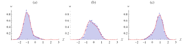
In our particular case, the minimization of the square of distance $D^{2}(|\alpha|,\varphi,\eta)$ results in $D^{2}=0.0436$ which is achieved at $|\alpha|_{\rm opt}=0.81$, $\varphi_{\rm opt}=3.14$, $\eta_{\rm opt}=0.58$. On substituting these parameters in formula (2), we can depict the closest theoretical quadrature distributions (see Fig. 1).

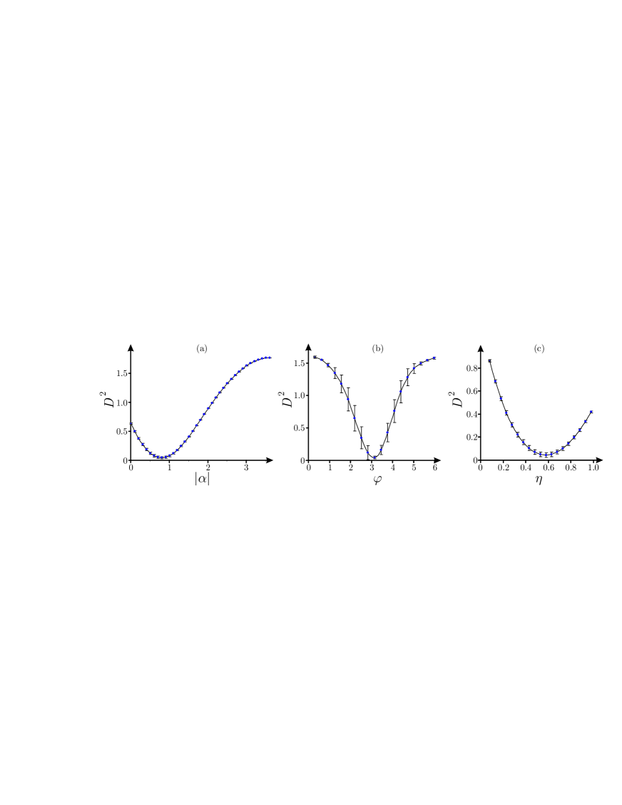
In order to evaluate the errors of estimated parameters $|\alpha|_{\rm opt}$, $\varphi_{\rm opt}$, and $\eta_{\rm opt}$ we consider three cuts of the function $D^{2}(|\alpha|,\varphi,\eta)$ that cross at the point $(|\alpha|_{\rm opt},\varphi_{\rm opt},\eta_{\rm opt})$. The values of function and their errors are shown in Fig. 2. Further, the error of an optimal parameter $q_{\rm opt}$ can be evaluated as $\Delta q/{\rm SNR}$, where $\Delta q$ is the width of the corresponding function cut and ${\rm SNR}=(\max D^{2}-\min D^{2})/\max\Delta(D^{2})$ plays the role of signal to noise ratio. The errors evaluated in such a way give rise to the following results: $|\alpha|_{\rm opt}=0.81\pm 0.03$, $\varphi_{\rm opt}=3.14\pm 0.25$, $\eta_{\rm opt}=0.58\pm 0.02$. The least precise parameter is the phase $\varphi$ and this can be attributed to the relatively small mean number of photons $\langle n\rangle\lesssim 1$ and imprecise fixing of the local oscillator phase $\theta$. Improving control of this parameter would result in higher precision of parameters under estimation.

4 Fidelity of detection

Sometimes, the Hilbert–Schmidt distance between the states is not very representative because it can grow under the action of quantum operations (not monotone metric). In this case one exploits some other quantities, e.g., the Bures distance $D_{\rm B}=\sqrt{2(1-F)}$, where $F={\rm Tr}\sqrt{\sqrt{\rho_{\rm th}}\rho_{\rm ex}\sqrt{\rho_{\rm th}}}$ is Uhlmann’s fidelity (see, e.g., the book [36]). The fidelity is difficult to express in operational way through quadrature distributions. Nevertheless, we can use recently found bounds for fidelity: the sub-fidelity $E$ and the super-fidelity $G$ satisfying $E\leq F^{2}\leq G$ and given by formulas [26, 37, 38]

$$E(\rho_{\rm th},\rho_{\rm ex})=\Tr\rho_{\rm th}\rho_{\rm ex}+\sqrt{2[(\Tr\rho_{\rm th}\rho_{\rm ex})^{2}-\Tr\rho_{\rm th}\rho_{\rm ex}\rho_{\rm th}\rho_{\rm ex}]},$$ (5)

$$G(\rho_{\rm th},\rho_{\rm ex})=\Tr\rho_{\rm th}\rho_{\rm ex}+\sqrt{\left(1-\Tr\rho_{\rm th}^{2}\right)\left(1-\Tr\rho_{\rm ex}^{2}\right)}.$$ (6)

Figure 2: Square of the Hilbert–Schmidt distance vs. state and detector parameters in the vicinity of the global minimum: $D^{2}(|\alpha|,\varphi_{\rm opt},\eta_{\rm opt})$ (a), $D^{2}(|\alpha|_{\rm opt},\varphi,\eta_{\rm opt})$ (b), $D^{2}(|\alpha|_{\rm opt},\varphi_{\rm opt},\eta)$ (c).

The overlap $\Tr\rho_{\rm th}\rho_{\rm ex}$ and purity $\Tr\rho_{\rm ex}^{2}$ are readily expressed through tomograms (see, e.g., [33]). It is worth noting that the purity can also be estimated by exploiting the covariant uncertainty relation [34]. As far as 4-product $\Tr\rho_{\rm th}\rho_{\rm ex}\rho_{\rm th}\rho_{\rm ex}$ is concerned, we can approximate it by $\Tr\rho_{\rm th}^{4}$. In fact, we have $|\Tr\rho_{\rm th}\rho_{\rm ex}\rho_{\rm th}\rho_{\rm ex}-\Tr\rho_{\rm th}^{4}|\leq|\Tr\rho_{\rm ex}\rho_{\rm th}\rho_{\rm ex}-\Tr\rho_{\rm th}^{3}|\leq|\Tr\rho_{\rm ex}^{2}-\Tr\rho_{\rm th}^{2}|$ and can modify the sub-fidelity as follows:

$$\!\!\!\!\!\!\!\!\!\!\!\!E^{\prime}(\rho_{\rm th},\rho_{\rm ex})=\Tr\rho_{\rm th}\rho_{\rm ex}+\sqrt{2[(\Tr\rho_{\rm th}\rho_{\rm ex})^{2}-\Tr\rho_{\rm th}^{4}-|\Tr\rho_{\rm ex}^{2}-\Tr\rho_{\rm th}^{2}|]}.$$ (7)

In order to be able to calculate the modified sub-fidelity (7) for SPACS, we find the following theoretical values:

$$\!\!\!\!\!\!\!\!\!\!\Tr\rho_{\rm th}^{2}=1-\frac{2\eta(1-\eta)}{(1+|\alpha|^{2})^{2}},\qquad\qquad\Tr\rho_{\rm th}^{4}=1-\frac{4\eta(1-\eta)}{(1+|\alpha|^{2})^{2}}+\frac{2\eta^{2}(1-\eta)^{2}}{(1+|\alpha|^{2})^{4}}.\qquad$$ (8)

Returning to the example considered earlier, we substitute the experimental data and the optimal theoretical values $|\alpha|_{\rm opt}=0.81$, $\varphi_{\rm opt}=3.14$, $\eta_{\rm opt}=0.58$ in formula (6) and obtain the upper bound $G(\rho_{\rm th},\rho_{\rm ex})=0.98\pm 0.02$. In our case, the direct calculation of sub-fidelity (7) turns out to be problematic because the confidence interval of the radicand is $[-0.07;0.05]$ (cf. $2[(\Tr\rho_{\rm th}^{2})^{2}-\Tr\rho_{\rm th}^{4}]=0.032$). Thus, the calculation of square root is worthless. Therefore, the use of formula (7) is possible only with the data of very high precision (errors should be substantially less than 1%). Whenever this does not happen, one can use another lower bound $E^{\prime\prime}=\Tr\rho_{\rm th}\rho_{\rm ex}\leq F^{2}$ (see, e.g., [26]). This lower bound is easy to calculate and in our case it equals $E^{\prime\prime}=0.81\pm 0.02$. Consequently, the fidelity of our interest is bounded by the two-sided inequality $0.81\pm 0.02\leq F^{2}\leq 0.98\pm 0.02$.

5 Conclusions

In order to estimate parameters of some prepared SPACS we developed the operational method whose essence was the comparison of experimental histograms with theoretically predicted quadrature distributions. The explicit form of theoretical distributions took into account the losses presented, which allowed us to infer not only the state parameter $\alpha$ but also the parameter $\eta$ describing the overall efficiency of homodyne detection. We discussed some practical issues concerning the easiest way to calculate the Hilbert–Schmidt distance and evaluate the errors of estimated parameters. The phase of the state turned out to be the least precise parameter, which could be ascribed to the small intensity of the signal mode and the errors in control of the local oscillator phase. Then we considered some operational techniques to determine the lower and upper bounds for fidelity of detection. We showed that, in practice, some of these bounds can be calculated only with highly precise data.

The outlook for further research is to use high sensitivity of homodyne detection to trace all the stages of quantum state’s life: its preparation, transformation via a quantum channel, and detection. Using appropriate theoretical models of these processes, one can determine the corresponding parameters. For instance, dark counts in the trigger detector result in mixing of the SPACS with a residual coherent state. In this case, the measured tomogram reads $(1-p)w_{\rm SPACS}+p\,w_{\rm coherent}$, where $p$ is a fraction of dark counts. The parameter $p$ can be estimated by the same algorithm of comparing $w_{\rm ex}$ and $w_{\rm th}$.

In general, optical tomograms can be valuable information sources on equal footing with other state descriptions [39]. Improving the accuracy of homodyne detection, one can check the validity of more complicated quantum theories and observe new phenomena (see, e.g., [29]). The role of SPACS states for new experiments can be also dramatic because of their ability to exhibit properties ranging from classical to quantum ones for different intensities [14].

References

- [1] Vogel K and Risken H 1989 Phys. Rev. A 40 2847
- [2] Smithey D T, Beck M, Raymer M G and Faridani A 1993 Phys. Rev. Lett. 70 1244
- [3] Schiller S, Breitenbach G, Pereira S F, Müller T and Mlynek J 1996 Phys. Rev. Lett. 77 2933
- [4] Polycarpou C, Cassemiro KN, Venturi G, Zavatta A and Bellini M 2012 Phys. Rev. Lett. 109 053602
- [5] Buono D, Nocerino G, Porzio A and Solimeno S 2012 Phys. Rev. A 86 042308
- [6] Leonhardt U 1997 Measuring the Quantum State of Light (Cambridge University Press, Cambridge)
- [7] Bachor H-A and Ralph T C 2004 A Guide to Experiments in Quantum Optics (2nd ed., WILEY-VCH Verlag, Weinheim) Section 8
- [8] Zavatta A, Viciani S and Bellini M 2006 Laser Phys. Lett. 3 3
- [9] Vogel W and Welsch D-G 2006 Quantum Optics (3rd revised and extended ed., WILEY-VCH Verlag, Weinheim) Sections 6 and 7
- [10] Walls D F and Milburn G J 2008 Quantum optics (2nd ed., Springer, Berlin)
- [11] Lvovsky A I and Raymer M G 2009 Rev. Mod. Phys. 81 299
- [12] Agarwal G S and Tara K 1991 Phys. Rev. A 43 492
- [13] Dodonov V V, Marchiolli M A, Korennoy Ya A, Man’ko V I and Moukhin Y A 1998 Phys. Rev. A 58 4087
- [14] Zavatta A, Viciani S and Bellini M 2004 Science 306 660
- [15] Zavatta A, Viciani S and Bellini M 2005 Phys. Rev. A 72 023820
- [16] Parigi V, Zavatta A, Kim M and Bellini M 2007 Science 317 1890
- [17] Kim M S, Jeong H, Zavatta A, Parigi V and Bellini M 2008 Phys. Rev. Lett. 101 260401
- [18] Zavatta A, Parigi V, Kim M S, Jeong H and Bellini M 2009 Phys. Rev. Lett. 103 140406
- [19] Kumar R, Barrios E, Kupchak C and Lvovsky A I 2012 Experimental characterization of bosonic photon creation and annihilation operators Preprint arXiv:1210.1150v1 [quant-ph]
- [20] Zavatta A, Parigi V and Bellini M 2007 Phys. Rev. A 75 052106
- [21] Parigi V, Zavatta A and Bellini M 2009 J. Phys. B: At. Mol. Opt. Phys. 42 114005
- [22] Kiesel T, Vogel W, Bellini M and Zavatta A 2011 Phys. Rev. A 83 032116
- [23] Zavatta A, Fiurášek J and Bellini M 2011 Nature Photonics 5 52
- [24] Bhattacharyya A 1943 Bull. Calcutta Math. Soc. 35 99
- [25] Filippov S N and Man’ko V I 2010 Phys. Scr. T140 014043
- [26] Miszczak J A, Puchała Z, Horodecki P, Uhlmann A and Życzkowski K 2009 Quantum Information and Computation 9 0103
- [27] Filippov S N and Man’ko V I 2011 Phys. Scr. 83 058101
- [28] Bellini M, Coelho A S, Filippov S N, Man’ko V I and Zavatta A 2012 Phys. Rev. A 85 052129
- [29] Pikovski I, Vanner M R, Aspelmeyer M, Kim M S and Brukner Č 2012 Nature Physics 8 393
- [30] Leonhardt U and Paul H 1993 Phys. Rev. A 48 4598
- [31] Ivan J S, Sabapathy K K and Simon R 2011 Phys. Rev. A 84 042311
- [32] Dodonov V V, Man’ko O V, Man’ko V I and Wünsche A 1999 Phys. Scr. 59 81
- [33] Man’ko M A and Man’ko V I 2011 AIP Conference Proceedings 1334 217
- [34] Man’ko V I, Marmo G, Porzio A, Solimeno S and Ventriglia F 2011 Phys. Scr. 83 045001
- [35] Korn G A and Korn T M 1968 Mathematical Handbook for Scientists and Engineers. Definitions, Theorems, and Formulas for Reference and Review (2nd enlarged and revised edition, McGraw-Hill, New York) Section 20.7-2
- [36] Bengtsson I and Życzkowski K 2006 Geometry of Quantum States (Cambridge University Press, New York) Section 13.3
- [37] Chen J-L, Fu L, Ungar A A and Zhao X-G 2002 Phys. Rev. A 65 054304
- [38] Mendonça P E M F, Napolitano R d J, Marchiolli M A, Foster C J and Liang Y-C 2008 Phys. Rev. A 78 052330
- [39] Ibort A, Man’ko V I, Marmo G, Simoni A and Ventriglia F 2009 Phys. Scr. 79 065013