Chiral Dynamics With Wilson Fermions

Abstract:

Close to the continuum the lattice spacing affects the smallest eigenvalues of the Wilson Dirac operator in a very specific manner determined by the way in which the discretization breaks chiral symmetry. These effects can be computed analytically by means of Wilson chiral perturbation theory and Wilson random matrix theory. A number of insights on chiral Dynamics with Wilson fermions can be obtained from the computation of the microscopic spectrum of the Wilson Dirac operator. For example, the unusual volume scaling of the smallest eigenvalues observed in lattice simulations has a natural explanation. The dynamics of the eigenvalues of the Wilson Dirac operator also allow us to determine the additional low energy constants of Wilson chiral perturbation theory and to understand why the Sharpe-Singleton scenario is only realized in unquenched simulations.

1 Introduction

In order to study the chiral limit in lattice QCD with Wilson Fermions, it is essential to understand the phase structure at nonzero lattice spacing. Since the continuum limit, $a\to 0$, and the chiral limit, $m\to 0$, do not commute, lattice spacing effects can induce new phase transitions which have no analogue in the continuum. These new phase structures are known as the Aoki phase [1] and the Sharpe-Singleton scenario [2]. The presence of new phase structures due to the lattice artifacts may at first appear to be a severe drawback for the application of Wilson fermions, however, these lattice artifacts can be turned to one’s favor: The Aoki phase is reached through a second order phase transition and just outside the Aoki phase the pions have dispersion relations which resemble those of almost massless quarks in the continuum.

Because the Wilson term breaks chiral symmetry the effects of the lattice spacing lead to new terms in chiral perturbation theory. This extended low energy theory is know as Wilson chiral perturbation theory. The precise form of the terms was worked out in [2, 4, 5] and at order $a^{2}$ involves three new low energy constants, which encode the severity of chiral symmetry breaking by the lattice artifacts. Recently a large number of new analytic results concerning chiral dynamics with Wilson fermions have been obtained from Wilson chiral perturbation theory by working from the perspective of the Wilson Dirac eigenvalues [6, 7, 8, 9, 10, 11, 12, 13, 14, 15, 16, 17]. The aim in this review is to give an introduction to the new understanding which the results has brought about rather than on the technical details.

We will focus on three of the most important new insights which follow from the results namely, 1) that the Sharpe-Singleton scenario is only realized in unquenched simulations, 2) that the $a/\sqrt{V}$ scaling of the smallest eigenvalues of the Hermitian Wilson Dirac operator, observed on the lattice [18, 19, 20], is a good sign, and finally 3) that the results offer a new way to measure the additional low energy constants of Wilson chiral perturbation theory.

Two new results are also included in this review. First, we determine the meta-stable region around the Sharpe-Singleton 1st order phase transition, and second we show that the sampling of the individual sectors is essential in order to determine the vacuum structure in the Aoki phase.

2 Wilson Chiral Perturbation Theory in the $\epsilon$-regime

The Wilson term in the Wilson Dirac operator

$$D_{W}=\frac{1}{2}\gamma_{\mu}(\nabla_{\mu}+\nabla_{\mu}^{*})-\frac{ar}{2}\nabla_{\mu}\nabla_{\mu}^{*}$$ (1)

breaks chiral symmetry. Therefore, the shortest length scale $a$ also affects the physics of longest length scale $1/m_{\pi}$. This effect is captured by Wilson chiral perturbation theory [3, 2, 4, 5], for which we now give a focused review.

As always in chiral perturbation theory it is essential to set up a counting scheme. Here we will work in the $\epsilon$-regime where the $V\to\infty$ limit is tied to the chiral and continuum limit such that

$$mV,\quad\zeta V,\quad{\rm and}\quad a^{2}V$$ (2)

are kept fixed and of order unity ($\zeta$ is the axial mass). The partition function of Wilson chiral perturbation theory at leading order then reduces to a group integral [21, 22]

$$Z_{N_{f}}(m,\zeta;a)=\int_{SU(N_{f})}dU~{}e^{S[U]},$$ (3)

where the action is

$$S = \frac{m}{2}\Sigma V{\rm Tr}(U+U^{\dagger})+\frac{\zeta}{2}\Sigma V{\rm Tr}(U-U^{\dagger})$$

$$-a^{2}VW_{6}[{\rm Tr}\left(U+U^{\dagger}\right)]^{2}-a^{2}VW_{7}[{\rm Tr}\left(U-U^{\dagger}\right)]^{2}-a^{2}VW_{8}{\rm Tr}(U^{2}+{U^{\dagger}}^{2}).$$

The convention for the low energy constants $W_{6}$, $W_{7}$ and $W_{8}$ is that of [6, 8]. In [5] these constants are denoted respectively by $-{W_{6}}^{\prime}$, $-{W_{7}}^{\prime}$ and $-{W_{8}}^{\prime}$.

As in the continuum [23] it is most useful to consider Wilson chiral perturbation theory in sectors with fixed index $\nu$, such that [6, 8]

$$Z_{N_{f}}^{\nu}(m,\zeta;a)=\int_{U(N_{f})}dU\ {\det}^{\nu}U~{}e^{S[U]},$$ (5)

where we obviously have

$$Z_{N_{f}}(m,\zeta;a)=\sum_{\nu}Z_{N_{f}}^{\nu}(m,\zeta;a).$$ (6)

The index defined in the above decomposition of the partition function is the index of the Wilson Dirac operator [6, 8]

$$\nu=\sum_{k}{\rm sign}(\langle k|\gamma_{5}|k\rangle),$$ (7)

where $|k\rangle$ is the eigenvector associated with the $k$’th real mode of the Wilson Dirac operator in the physical branch. We will make explicit use of this index in section 7 where we discuss the microscopic spectral density. In the first sections we will work at mean field level where the dependence on the index is suppressed.

From the action in Eq. (2) it is clear that the partition function in the $\epsilon$-regime of Wilson chiral perturbation theory only depends on the dimensionless scaling variables

$$\hat{m}=mV\Sigma,\qquad\hat{\zeta}=\zeta V\Sigma\quad{\rm and}\qquad\hat{a}_{i}^{2}=a^{2}VW_{i}.$$ (8)

The mean field limit corresponds to the saddle point approximation to the group integral in the limit where these dimensionless numbers are all much larger than unity.

     

Figure 1: The mean field potential for the orientation of the vacuum. When $\cos(\theta)=\pm 1$ the lattice simulation is in the normal phase with the standard chiral condensate. Left $W_{8}+2W_{6}>0$: The Aoki phase develops when the minimum of the potential is between -1 and 1. Right $W_{8}+2W_{6}<0$: For the Sharpe-Singleton scenario the minimum is always at -1 or 1. The additional meta-stable minimum at $\cos(\theta)=-1$ (red curve) becomes degenerate with the minimum at $\cos(\theta)=1$ for $m=0$ (blue curve) resulting in the 1st order Sharpe-Singleton phase transition. The parameters chosen for the plots are $\hat{m}=10,5,0$ and $8(\hat{a}_{8}^{2}+2\hat{a}_{6}^{2})=\pm 4$.

3 Aoki phase and Sharpe-Singleton scenario

The form of the order $a^{2}$ terms in Wilson chiral perturbation theory are uniquely determined by the way in which the Wilson term breaks chiral symmetry. Each of the three new terms comes with a new low energy constant, the value of which is not fixed by the flavor symmetries. The sign of these three additional low energy constants, however, is determined by the $\gamma_{5}$-Hermiticity of the Wilson Dirac operator

$$\gamma_{5}D_{W}\gamma_{5}=D_{W}^{\dagger}.$$ (9)

Only for

$$W_{6}<0,\qquad W_{7}<0\qquad{\rm and}\qquad W_{8}>0$$ (10)

does the Wilson chiral Lagrangian describe lattice QCD with a $\gamma_{5}$-Hermitian Wislon Dirac operator [6, 8, 24, 14]. As we shall now demonstrate these signs give vital information on how the Aoki phase and the Sharpe-Singleton scenario are realized. To show this let us first work out the phase structure of lattice QCD with Wilson fermions at small $m$ and $a$ using Wilson chiral perturbation theory at mean field level. With the mean field ansatz for the orientation of the Goldstone field [2] (here and below we focus on the case of two mass degenerate flavors)

$$U=\cos(\theta)+i\sin(\theta)\sigma_{3}$$ (11)

we find the mean field action

$$S_{MF}=2\hat{m}\cos(\theta)-4\hat{a}_{8}^{2}(2\cos^{2}(\theta)-1)-16\hat{a}_{6}^{2}\cos^{2}(\theta).$$ (12)

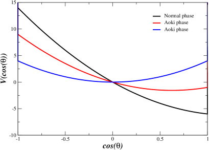
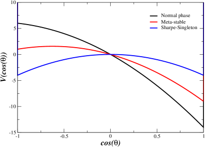
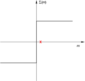
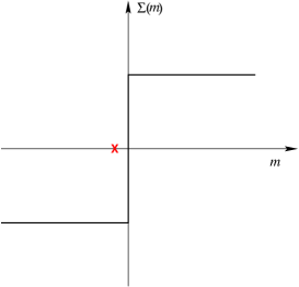
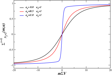
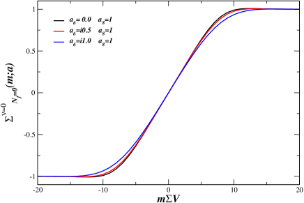
This effective potential for $\cos(\theta)$ is plotted in figure 1 for the two cases $W_{8}+2W_{6}>0$ (l.h.s.) and $W_{8}+2W_{6}<0$ (r.h.s.). In the first case the orientation, as given by $\cos(\theta)$, continuously moves from 1 to -1 as a function of the quark mass. This is the Aoki phase [1]. In the second case, where $W_{8}+2W_{6}<0$, the orientation jumps from 1 to -1 at $m=0$. This is the first order Sharpe-Singleton phase transition [2].

The pion masses for $|m|\Sigma>8(W_{8}+2W_{6})a^{2}$ are given by the order-$a^{2}$ corrected GOR-relation [2, 25]

$$\frac{m_{\pi}^{2}F_{\pi}^{2}}{2}=|m|\Sigma-8(W_{8}+2W_{6})a^{2}.$$ (13)

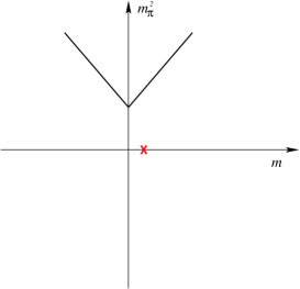
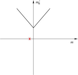
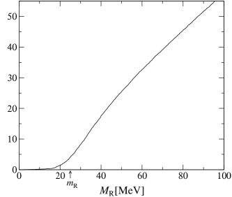
Approaching the Aoki-phase (where $W_{8}+2W_{6}>0$) the squared mass of the pions goes to zero linearly with the quark mass. If we absorb the order $a^{2}$-correction into the quark mass this behavior of the pion masses is just like in the continuum. On the contrary in the Sharpe-Singleton scenario (where $W_{8}+2W_{6}<0$) the pion mass is always positive. See the rightmost panels of figure 3 and figure 5 respectively.

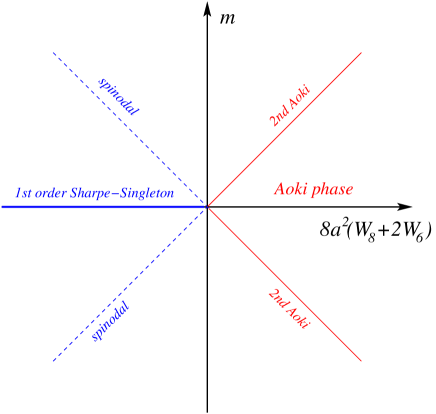
Since the Sharpe-Singleton scenario involves a first order phase transition it is natural to ask: What is the meta-stable region? The answer is readily seen from Eq. (12) or graphically from the r.h.s. of figure 1. The spinodal line occurs when the maximum of the effective potential enters between $-1$ and $1$. That is, at exactly the same quark mass as the Aoki phase would have occurred for the opposite sign of $W_{8}+2W_{6}$. This is illustrated in figure 2.

Figure 2: The phase diagram for lattice QCD with Wilson fermions in the $(8(W_{8}+2W_{6})a^{2},m)$-plane. For positive values of $8a^{2}(W_{8}+2W_{6})$ the Aoki phase dominates with the 2nd order phase transition at $|m|=8a^{2}(W_{8}+2W_{6})$ and associated Goldstone modes for smaller values of $|m|$. With negative values of $8a^{2}(W_{8}+2W_{6})$ the Sharpe-Singleton scenario dominates with the 1st order phase transition at $m=0$ and spinodal lines at $|m|=|8a^{2}(W_{8}+2W_{6})|$. The meta-stable region is hence between the dashed blue lines.

4 A puzzle

The above analysis shows that either the Aoki phase or the Sharpe-Singleton scenario will dominate if we take the chiral limit prior to the continuum limit. Which of the two is realized, depends on whether $W_{8}$ is more positive than $2W_{6}$ is negative and hence on the details of the specific lattice simulation in question. This analysis was extended to the quenched case in [26] where it was argued that the Aoki phase and the Sharpe-Singleton scenario potentially both should be realizable also in quenched simulations. On the lattice, however, quenched lattice simulations consistently observe the Aoki phase [27, 29, 28, 30], while in unquenched simulations both the Aoki and the Sharpe-Singleton scenario are observed [31, 32, 33, 18, 19, 20, 34, 35, 36, 37, 38, 39, 40, 41]. As we now show this puzzle has a natural solution when we consider the problem from the perspective of the Wilson Dirac eigenvalues.

Figure 3: The physical branch of the spectral density of the Wilson Dirac operator (left) the chiral condensate (middle) and the pion mass (right). The vertical dashed lines mark the support of the eigenvalue density of the Wilson Dirac operator. The location is at $|Re[z]|\Sigma=8(W_{8}+2W_{6})a^{2}$. The Aoki phase occours when the quark mass is between the two dashed lines ($W_{8}+2W_{6}>0$). In addition there is one massive mode inside the Aoki phase.

5 Spectrum of the Wilson Dirac operator for $W_{6}=W_{7}=0$

We now derive the spectral density of the Wilson Dirac operator. Let us start with the case where $W_{6}=W_{7}=0$. In this case $W_{8}+2W_{6}>0$, since $W_{8}>0$ by the $\gamma_{5}$-Hermiticity of the Wilson Dirac operator, and we have the Aoki phase.

Because of the $\gamma_{5}$-Hermiticity the eigenvalues of the Wilson Dirac operator are either purely real or come in complex conjugate pairs [42]. For a scatter plot of the eigenvalues, see for example [43]. In order to derive the spectral density of the Wilson Dirac operator in the complex plane

$$\rho_{c,N_{f}}(z,z^{*})=\langle\sum_{i}\delta^{2}(\lambda^{W}_{i}-z)\rangle_{N_{f}}$$ (14)

from Wilson chiral perturbation theory we therefore need to extend the partition function into a replicated generating functional with $p$ additional pairs of conjugate quarks with masses $\hat{z}$ and $\hat{z}^{*}$,

$$Z_{N_{f}+2p}^{\nu}(\hat{z},\hat{z}^{*},\hat{m};\hat{a}_{i})=\langle\prod_{i}(\lambda^{W}_{i}-m)\prod_{i}(\lambda^{W}_{i}-z)^{p}((\lambda^{W}_{i})^{*}-z^{*})^{p}\rangle.$$ (15)

The eigenvalue density of the Wilson Dirac operator in the complex plane is then obtained as

$$\rho_{c,N_{f}}^{\nu}(\hat{z},\hat{z}^{*},\hat{m};\hat{a}_{i}) = \partial_{\hat{z}^{*}}\lim_{p\to 0}\partial_{\hat{z}}\frac{1}{p}\log Z_{N_{f}+2p}^{\nu}(\hat{z},\hat{z}^{*},\hat{m};\hat{a}_{i}).$$ (16)

The trick is now to use the low energy effective theory, ie. Wilson chiral perturbation theory, to compute the replicated generating functional and thereby obtain the density. For an introduction to the use of the replica method in chiral perturbation theory, see [44].

The low energy limit of the replicated generating functional is given by Wilson chiral perturbation theory with the mass matrix

$${\cal M}={\rm diag}(\hat{m}_{N_{f}},\hat{z}_{p},\hat{z}^{*}_{p}),$$ (17)

where the subscript on the quark masses refers to the number of times the specific mass appears. In the mean field limit the dependence on the number, $p$, of replica flavors is trivial for $W_{6}=W_{7}=0$, and one simply obtains (we use the notation $\hat{z}=\hat{x}+i\hat{y}$)

$$\rho_{c,N_{f}=2}^{\rm MF}(\hat{x},\hat{m};\hat{a}_{8})=\theta(8\hat{a}_{8}^{2}-|\hat{x}|).$$ (18)

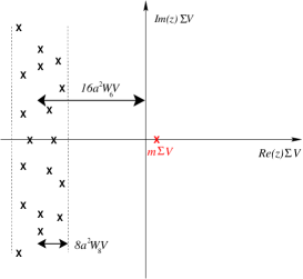
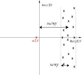
Note that the eigenvalue density is independent of the imaginary part of the eigenvalue, hence it forms a strip along the imaginary axis of width $8\hat{a}_{8}^{2}$. The Aoki-phase sets in when the quark mass enters the eigenvalue strip, as in figure 3.

The microscopic limit of both the eigenvalue density of $D_{W}$ in the complex plane and on the real axis was worked out in [6, 8, 11, 14], see figure 4. The exact way in which the real eigenvalues are distributed shows at which value of the quark mass the simulations are safe from exceptional configurations.

Figure 4: Left: The microscopic eigenvalue density of the Wilson Dirac operator in the complex plane (in the sector with $\nu=0$ for $N_{f}=0$ and $a\sqrt{W_{8}V}=0.75$, $W_{6}=W_{7}=0$) and Right: the microscopic eigenvalue density of the real eigenvalues of the Wilson Dirac operator (in the sectors with $\nu=1,2,3$ for $N_{f}=0$ and $a\sqrt{W_{8}V}=0.2$, $W_{6}=W_{7}=0$). The exponential fall-off of the eigenvalue density is essential to avoid exceptional configurations.

6 The realization of the Sharpe-Singleton scenario: The solution to the puzzle

Figure 5: The realization of the Sharpe-Singleton scenario ($W_{8}+2W_{6}<0$). The red cross marks the size of the quark mass top: the mass is positive and below: the mass is negative. As the quark mass changes sign the strip of eigenvalues jumps across the origin and consequently the chiral condensate has a first order discontinuity at $m=0$, cf. the middle panels. Since the quark mass never reaches the eigenvalue density the pions remain massive even at $m=0$. See the rightmost figures. Clearly this scenario is only possible in the unquenched theory where the eigenvalue density can depend on the quark mass.

Let us now compute the effect of $W_{6}$ on the spectral density of $D_{W}$ in the mean field limit. To do so it is useful first to linearize the square in the $W_{6}$ term of the replicated generating functional with a Gaussian integral over a fluctuating mass $y_{6}$. This leads to [14]

$$\rho_{c,N_{f}}^{\nu}(\hat{z},\hat{z}^{*},\hat{m};\hat{a}_{6},\hat{a}_{8}) = \frac{1}{Z_{N_{f}}^{\nu}(\hat{m};\hat{a}_{6},\hat{a}_{8})}\int[dy_{6}]\ Z_{N_{f}}^{\nu}(\hat{m}-y_{6};\hat{a}_{8})\rho_{c,N_{f}}^{\nu}(\hat{z}-y_{6},\hat{z}^{*}-y_{6},\hat{m}-y_{6};\hat{a}_{8}),$$

where we used the notation $[dy_{6}]=dy_{6}/(4\sqrt{\pi}|\hat{a}_{6}|)\exp(-y_{6}^{2}/(16|\hat{a}_{6}^{2}|))$. This expresses the eigenvalue density of $D_{W}$ in the complex plane at $W_{6}\neq 0$ in terms of the eigenvalue density with $W_{6}=0$.

At the mean field level for $N_{f}=2$, using Eq. (18), we get

$$\rho_{c,N_{f}=2}^{\rm MF}(\hat{x},\hat{m};\hat{a}_{6},\hat{a}_{8})=\frac{1}{Z_{2}^{\rm MF}(\hat{m};\hat{a}_{6},\hat{a}_{8})}\int dy_{6}\ e^{-y_{6}^{2}/16|\hat{a}_{6}^{2}|}Z_{2}^{\rm MF}(\hat{m}-y_{6};\hat{a}_{8})\theta(8\hat{a}_{8}^{2}-|\hat{x}-y_{6}|),$$ (20)

where

$$Z_{2}^{\rm MF}(\hat{m};\hat{a}_{6},\hat{a}_{8}) = e^{2\hat{m}+16|\hat{a}_{6}^{2}|-4\hat{a}_{8}^{2}}+e^{-2\hat{m}+16|\hat{a}_{6}^{2}|-4\hat{a}_{8}^{2}}$$

$$+\theta(8(\hat{a}_{8}^{2}+2\hat{a}_{6}^{2})-|\hat{m}|)e^{\hat{m}^{2}/8(\hat{a}_{8}^{2}-2|\hat{a}_{6}^{2}|)+4\hat{a}_{8}^{2}}.$$

This saddle point structure of the two flavor partition function leads to

$$\rho_{c,N_{f}=2}^{\rm MF}(\hat{x},\hat{m};\hat{a}_{6},\hat{a}_{8}) = \frac{1}{Z_{2}^{\rm MF}(\hat{m};\hat{a}_{6},\hat{a}_{8})}$$

$$\times\Big{\{}e^{2\hat{m}+16|\hat{a}_{6}^{2}|-4\hat{a}_{8}^{2}}\theta(8\hat{a}_{8}^{2}-|\hat{x}+16|\hat{a}_{6}|^{2}|)$$

$$+e^{-2\hat{m}+16|\hat{a}_{6}^{2}|-4\hat{a}_{8}^{2}}\theta(8\hat{a}_{8}^{2}-|\hat{x}-16|\hat{a}_{6}|^{2}|)$$

$$+\theta(8(\hat{a}_{8}^{2}+2\hat{a}_{6}^{2})-|\hat{m}|)\theta\left(8\hat{a}_{8}^{2}-\left|\hat{x}+\frac{2|\hat{a}_{6}|^{2}\hat{m}}{(\hat{a}_{8}^{2}-2|\hat{a}_{6}|^{2})}\right|\right)e^{\hat{m}^{2}/8(\hat{a}_{8}^{2}-2|\hat{a}_{6}^{2}|)+4\hat{a}_{8}^{2}}\Big{\}}.$$

Since we seek to understand the realization of the Sharpe-Singleton scenario let us consider $W_{8}+2W_{6}<0$. The density in this case is shown in figure 5. As the quark mass changes sign the strip of eigenvalues jump from one side of the origin to the opposite side and this causes the 1st order jump of the chiral condensate. This explains how the Sharpe-Singleton scenario is realized in terms of the strong mass dependence of the unquenched eigenvalue density.

In the quenched case on the contrary the eigenvalue density is independent of the quark mass since the fermion determinant is absent in the measure. The quark mass in the quenched case, therefore, necessarily passes through the eigenvalue density and this leads to the standard Aoki phase, independent of the sign of $W_{8}+2W_{6}$. This explains why the Aoki phase is observed consistently in quenched simulations and thus solves the puzzle of section 4. One can also compute the quenched chiral condensate directly from the graded version of the partition function in Wilson chiral perturbation theory and reach the same conclusion. This is illustrated in figure 6. The analysis of [26] reached the conclusion that the Sharpe-Sharpe-Singleton scenario could be realized in quenched simulations because the bound on the signs of the $W_{i}$’s due to $\gamma_{5}$-Hermiticity had not been understood at the time.

The meta-stable region surrounding the 1st order Sharpe-Singleton phase transition (see figure 2) can also be observed in the eigenvalue density. For $0<m\Sigma<|W_{8}+2W_{6}|a^{2}$ and $W_{8}+2W_{6}<0$ the meta-stable minimum of $Z_{2}^{\rm MF}$ introduces a local minimum of the $y_{6}$ integral in Eq. (6). This local minimum offers the possibility for the strip of eigenvalues to temporarily jump to the opposite side of the origin thus inducing a fluctuating sign of the chiral condensate. Such fluctuations become more frequent as the meta-stable and global minimum of $Z_{2}^{\rm MF}$ become almost degenerate, ie. as $m$ approaches zero. Thus the meta-stability of the eigenvalue density is completely consistent with the meta-stability of the chiral condensate obtained directly from Eq. (12).

It is also instructive to consider the distance from the quark mass to the edge of the strip of eigenvalues of $D_{W}$. From Eq. (6) we see that this distance is given by

$$|m|-8(W_{8}+2W_{6})a^{2}/\Sigma.$$ (23)

This is exactly the combination which enters the right hand side of the order-$a^{2}$ corrected GOR relation, cf. Eq. (13). The distance from the quark mass to the edge of the strip of eigenvalues of $D_{W}$ can therefore be thought of as the effective quark mass which enters the standard continuum form of the GOR relation.

In the Sharpe-Singleton scenario, ie. for $W_{8}+2W_{6}<0$, the quark mass never reaches the strip of eigenvalues of $D_{W}$. The minimal distance between the quark mass and the eigenvalues is given by $-8(W_{8}+2W_{6})a^{2}$ and hence the smallest value which the pion mass can reach is

$$m_{\pi}=\sqrt{-16(W_{8}+2W_{6})a^{2}/F_{\pi}^{2}}.$$ (24)

This is of course exactly the same minimal value of the pion mass found in [2]. We now understand how this minimum is linked to the behavior of the eigenvalue density in the unquenched theory.

Figure 6: The Sharpe-Singleton first order phase transition is only realized in the unquenched theory. Here we show the mass dependence of the microscopic chiral condensate for $\hat{a}_{8}=1$ and $\hat{a}_{6}=0,0.5i$ and $i$ corresponding to $W_{8}+2W_{6}>0$, $W_{8}+2W_{6}=0$ and $W_{8}+2W_{6}<0$, respectively. Left $N_{f}=2$: The 1st order Sharpe-Singleton phase transition develops with the increasingly negative value of $W_{6}$. Right $N_{f}=0$: The smooth behavior of the chiral condensate as a function of the quark mass characteristic of the Aoki phase is present in the quenched theory even when $W_{8}+2W_{6}<0$.

7 Spectrum of the Hermitian Wilson Dirac operator

The $\gamma_{5}$-Hermiticity of the Wilson Dirac operator makes it natural to introduce the Hermitian Wilson Dirac operator, $D_{5}$, defined by

$$D_{5}\equiv\gamma_{5}(D_{W}+m)~{}.$$ (25)

There is a close analogue of the Banks Casher relation [45] for the spectrum of $D_{5}$: The lattice artifacts induce eigenvalues of $D_{5}$ with magnitude less than $|m|$ and when these build up a density at zero the Aoki phase is reached [46]. It is therefore essential to understand analytically the dependence of the smallest eigenvalues of the Hermitian Wilson Dirac operator in order to study chiral dynamics in simulations with Wilson fermions.

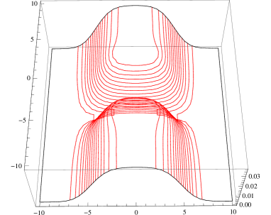
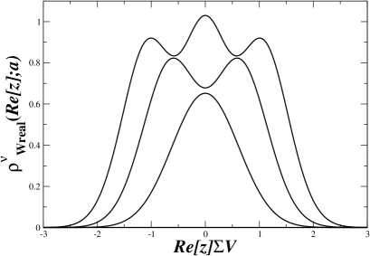
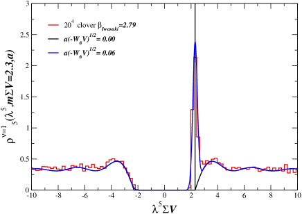
The first to consider the spectral density of $D_{5}$ from the perspective of Wilson chiral perturbation theory was Sharpe [47]. By now a detailed analytic understanding of the effects the discretization errors have on the spectrum of $D_{5}$ have been obtained [6, 8, 9, 10, 11, 12, 13, 14, 15, 16, 17]. A plot of the spectral density is shown in figure 7. The plot shows the density in the sector with $\nu=1$ and the index peak at $m$ is clearly visible. Also the precise way the eigenvalues intrude into the region between $-m$ and $m$ can be observed.

The predictions also offer a new way to measure the low energy constants of Wilson chiral perturbation theory [17, 48, 49, 50]: The histogram in figure 7 displays lattice data and the match of the analytic prediction to the lattice data fixes the values of the low energy constants. We refer to [50] for details.

One can also obtain the low energy constants from a fit of the analytic predictions for the spectral density of $D_{W}$ to lattice data. However, since $D_{5}$ is Hermitian it is somewhat easier to determine this spectrum numerically in lattice simulations. See also [51] for an alternative way to measure the $W_{i}$’s.

Figure 7: Red histogram: The spectral density of the Hermitian Wilson Dirac operator on quenched $20^{4}$ lattices in the sector with $\nu=1$. The eigenvalues have been rescaled with $\Sigma V/a=220$. See [50] for details about the simulations. Blue curve: The microscopic spectral density obtained from Wilson chiral perturbation theory with $N_{f}=0$, $\nu=1$, $\hat{m}=2.3$ and $\hat{a}_{6}=0.06$. Also shown is the black curve obtained from ordinary chiral perturbation theory with $a=0$. The prime effect of the lattice artifacts for $ha_{i}\ll 1$ is to smear the index-peak. This leads to the $a/\sqrt{V}$ scaling of the width of the smallest eigenvalue of the Hermitian Wilson Dirac operator reported in [18, 19].

Figure 8: The accumulated single eigenvalue distributions of the lowest eigenvalues of the Hermitian Wilson Dirac operator. Plot adopted from [49].

         

Figure 9: The accumulated eigenvalue density the Hermitian Wilson Dirac operator including all sectors. Left: quenched lattice simulation from [52]. Right: example of the analytic prediction from Wilson chiral perturbation theory in the $\epsilon$ regime with $N_{f}=0$. The parameters chosen for this example are $m\Sigma V=3$, $\hat{a}_{8}=0.2$ and $W_{6}=W_{7}=0$.

8 Scaling with $a/\sqrt{V}$

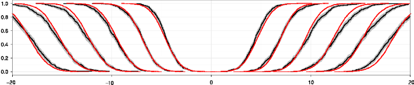
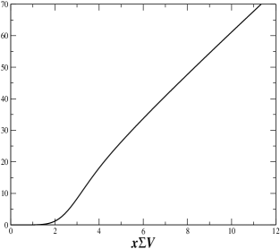
In the simulations of [18, 19, 20] it was found that the width of the distribution of the smallest eigenvalue of $D_{5}$ scales with $a/\sqrt{V}$. At first sight this may sound disturbing, since the Banks-Casher relations [45, 46] suggests that the smallest eigenvalues should scale with $1/V$. Hence one might fear that the $a/\sqrt{V}$-scaling is a sign of uncontrolled lattice artifacts, such as local defects not described by Wilson chiral perturbation theory. On the contrary, the $a/\sqrt{V}$ scaling is a good sign: In the limit where $\hat{a}_{i}\ll 1$ the smallest eigenvalues of $D_{5}$ should in fact scale precisely with $a/\sqrt{V}$ [6, 8]. For $\hat{a}_{i}\ll 1$ the primary influence of the lattice artifacts is to smear the topological mode into a peak around $m$ of width $a/\sqrt{V}$, as shown in figure 7. This fact, obtained from Wilson chiral perturbation theory, has been demonstrated explicitly in lattice quenched simulations [48, 49, 50]. See figures 7 and 8. Note that these lattice simulations were separated into sectors with fixed index. The effect of the discretization error on the spectrum of $D_{5}$ can also be studied without the separation into sectors. In figure 9 the accumulated eigenvalue density including all sectors is shown. The left hand plot is lattice data obtained in [52] while the right hand plot gives an example of the analytic results. It would be most interesting to preform a systematic fit to the data including the leading order corrections to the slope at large $\lambda^{5}$ obtained in [17].

9 Alternative vacuum in the Aoki phase for $N_{f}=2$

In [53] it was proposed that the additional condensate $\langle i\bar{u}\gamma_{5}u+i\bar{d}\gamma_{5}d\rangle$ will take a nonzero expectation value inside the Aoki phase along with the standard Aoki condensate $\langle i\bar{u}\gamma_{5}u-i\bar{d}\gamma_{5}d\rangle$. This suggestion is particularly interesting since the presence of the additional condensate is in direct contradiction with the results of Wilson chiral perturbation theory [54]. The additional condensate $\langle i\bar{u}\gamma_{5}u+i\bar{d}\gamma_{5}d\rangle$ is zero in the $\epsilon$-regime of Wilson chiral perturbation theory, Eq. (3), because it is the v.e.v. of ${\rm Tr}(U-U^{\dagger})$ which vanishes in $SU(2)$ where ${\rm Tr}U={\rm Tr}U^{\dagger}$. With fixed index, however, the group average is extended to $U(2)$ and ${\rm Tr}(U-U^{\dagger})$ does not vanish trivially. The behavior of $\langle i\bar{u}\gamma_{5}u+i\bar{d}\gamma_{5}d\rangle$ at fixed index can be examined by explicit evaluation of $U(2)$ integral  Eq. (5) and differentiation w.r.t. $\zeta$. One can also evaluate the squared condensate $\langle(i\bar{u}\gamma_{5}u+i\bar{d}\gamma_{5}d)^{2}\rangle$ at zero external sources as suggested in [55]. Again this is zero in SU(2) and nonzero at fixed index. As should of course be true, one recovers the vanishing value of the additional condensates within Wilson chiral perturbation theory, after a careful summation over all sectors with the appropriate partition functions as weights. In simulations, however, it can be very tricky to control this sum over the sectors. Even a small error in the sampling of the sectors can lead to a substantial error in the value of the additional condensates after summation over the sectors. The summation over the sectors become particularly delicate in the Aoki region if the low energy constant $W_{7}$ is non-vanishing. The reason is that the term proportional to $W_{7}$ is tantamount to a Gaussian fluctuating source for $i\bar{u}\gamma_{5}u+i\bar{d}\gamma_{5}d$. In other words, Wilson chiral perturbation theory predicts that it is essential to sample all the sectors with the correct weight in order to determine if the additional condensate is present.

10 Conclusion

The approach to chiral dynamics with Wilsons fermions from the perspective of the eigenvalues of the Wilson Dirac operator has lead to several new insights. On the macroscopic level it becomes clear that the Sharpe-Singleton scenario can only be realized in unquenched theories and on the microscopic scale we learn that the $a/\sqrt{V}$ scaling of the smallest eigenvalues of the Hermitian Wilson Dirac operator is a sign that the simulation is very close to the continuum. On a more technical but equally important level we now understand that the signs of the additional low energy constants in Wilson chiral perturbation theory are fixed. Moreover, the new analytic results offers a practical way to measure the additional low energy constants in lattice simulations. These combined new insights can be most useful when we seek to minimize discretization errors in lattice simulations with Wilson fermions. For example, to minimize $W_{8}+2W_{6}$ it is useful to know that the two contributions have opposite signs.

A control of the lattice artifacts becomes particularly important in studies of QCD with a larger number of flavors: In a mean field approach the coefficient in front of $W_{6}$ and $W_{7}$ scales with $N_{f}^{2}$ compared to the linear scaling of the $W_{8}$ term. This suggest that simulations with a larger number of flavors should be more likely to end up in the Sharpe-Singleton scenario. Hence one is less likely to be able to exploit the massless modes at the boundary of the Aoki phase to mimic the chiral limit for larger number of flavors.

Many aspects discussed in this review of chiral dynamics with Wilson fermions has a direct analogue for staggered fermions. It would be interesting to pursue this further. The necessary tools are already available [56] and first results have appeared [57]. The spectral properties of the Dirac operator could also cast additional light on simulation with mixed actions, see eg. [58].

Acknowledgments: I would like to thank the organizers of Lattice 2012 for an excellent conference and the chance to review these results in the plenary session. Furthermore, it is a great pleasure to thank Poul Henrik Damgaard, Jac Verbaarschot, Gernot Akemann, Urs Heller and Mario Kieburg for the collaborations leading to the publications this review is based upon. Joyce Myers is thanked for useful comments on the manuscript. This work was supported by the Sapere Aude program of The Danish Council for Independent Research.

References

- [1] S. Aoki, Phys. Rev. D30, 2653 (1984).
- [2] S. R. Sharpe and R. L. Singleton, Phys. Rev. D 58, 074501 (1998) [hep-lat/9804028].
- [3] M. Creutz, hep-lat/9608024.
- [4] G. Rupak and N. Shoresh, Phys. Rev. 66, 054503 (2002), [arXiv:hep-lat/0201019].
- [5] O. Bär, G. Rupak and N. Shoresh, Phys. Rev. D 70, 034508 (2004), [arXiv:hep-lat/0306021].
- [6] P. H. Damgaard, K. Splittorff and J. J. M. Verbaarschot, Phys. Rev. Lett. 105, 162002 (2010). [arXiv:1001.2937 [hep-th]].
- [7] G. Akemann, P. H. Damgaard, K. Splittorff, J. J. M. Verbaarschot, PoS LATTICE2010, 079 (2010). [1011.5121 [hep-lat]].
- [8] G. Akemann, P. H. Damgaard, K. Splittorff, J. J. M. Verbaarschot, Phys. Rev. D 83, 085014 (2011) [1012.0752 [hep-lat]].
- [9] K. Splittorff and J. J. M. Verbaarschot, Phys. Rev. D 84, 065031 (2011) [arXiv:1105.6229 [hep-lat]].
- [10] G. Akemann and T. Nagao, JHEP 1110, 060 (2011) [arXiv:1108.3035 [math-ph]].
- [11] M. Kieburg, J. J. M. Verbaarschot and S. Zafeiropoulos, Phys. Rev. Lett. 108, 022001 (2012) [arXiv:1109.0656 [hep-lat]].
- [12] R. N. Larsen, Phys. Lett. B 709, 390 (2012) [arXiv:1110.5744 [hep-th]].
- [13] K. Splittorff and J. J. M. Verbaarschot, Phys. Rev. D 85, 105008 (2012) [arXiv:1201.1361 [hep-lat]].
- [14] M. Kieburg, K. Splittorff and J. J. M. Verbaarschot, Phys. Rev. D 85, 094011 (2012) [arXiv:1202.0620 [hep-lat]].
- [15] G. Akemann and A. C. Ipsen, JHEP 1204, 102 (2012) [arXiv:1202.1241 [hep-lat]].
- [16] M. Kieburg, J. Phys. A A 45, 205203 (2012) [arXiv:1202.1768 [math-ph]].
- [17] S. Necco and A. Shindler, JHEP 1104, 031 (2011) [arXiv:1101.1778 [hep-lat]]; PoS LATTICE 2011, 250 (2011) [arXiv:1108.1950 [hep-lat]].
- [18] L. Del Debbio, L. Giusti, M. Luscher, R. Petronzio and N. Tantalo, JHEP 0702, 082 (2007) [hep-lat/0701009].
- [19] L. Del Debbio, L. Giusti, M. Luscher, R. Petronzio and N. Tantalo, JHEP 0702, 056 (2007) [hep-lat/0610059].
- [20] L. Del Debbio, L. Giusti, M. Luscher, R. Petronzio and N. Tantalo, JHEP 0602, 011 (2006) [hep-lat/0512021].
- [21] A. Shindler, Phys. Lett. B 672, 82 (2009) [arXiv:0812.2251 [hep-lat]].
- [22] O. Bär, S. Necco, and S. Schaefer, J. High Energy Phys. 03 (2009) 006.
- [23] H. Leutwyler and A. V. Smilga, Phys. Rev. D 46, 5607 (1992).
- [24] M. T. Hansen and S. R. Sharpe, Phys. Rev. D 85, 014503 (2012) [arXiv:1111.2404 [hep-lat]].
- [25] S. Aoki, Phys. Rev. D 68, 054508 (2003) [hep-lat/0306027].
- [26] M. Golterman, S. R. Sharpe and R. L. Singleton, Phys. Rev. D 71, 094503 (2005) [arXiv:hep-lat/0501015].
- [27] S. Aoki and A. Gocksch, Phys. Rev. D 45, 3845 (1992).
- [28] S. Aoki and A. Gocksch, Phys. Lett. B 231, 449 (1989).
- [29] S. Aoki and A. Gocksch, Phys. Lett. B 243, 409 (1990).
- [30] K. Jansen et al. [XLF Collaboration], Phys. Lett. B 624, 334 (2005) [arXiv:hep-lat/0507032].
- [31] S. Aoki, A. Ukawa and T. Umemura, Phys. Rev. Lett. 76, 873 (1996) [hep-lat/9508008].
- [32] S. Aoki, Nucl. Phys. Proc. Suppl. 60B, 206 (1998) [hep-lat/9707020].
- [33] E. -M. Ilgenfritz, W. Kerler, M. Muller-Preussker, A. Sternbeck and H. Stuben, Phys. Rev. D 69, 074511 (2004) [hep-lat/0309057].
- [34] T. Ishikawa et al. [JLQCD Collaboration], Phys. Rev. D 78, 011502 (2008) [arXiv:0704.1937 [hep-lat]].
- [35] S. Borsanyi, S. Durr, Z. Fodor, C. Hoelbling, S. D. Katz, S. Krieg, D. Nogradi and K. K. Szabo et al., JHEP 1208, 126 (2012) [arXiv:1205.0440 [hep-lat]].
- [36] S. Aoki et al. [JLQCD Collaboration], Phys. Rev. D 72, 054510 (2005) [hep-lat/0409016].
- [37] F. Bernardoni, J. Bulava and R. Sommer, PoS LATTICE 2011, 095 (2011) [arXiv:1111.4351 [hep-lat]].
- [38] F. Farchioni, R. Frezzotti, K. Jansen, I. Montvay, G. C. Rossi, E. Scholz, A. Shindler and N. Ukita et al., Eur. Phys. J. C 39, 421 (2005) [hep-lat/0406039].
- [39] F. Farchioni, K. Jansen, I. Montvay, E. Scholz, L. Scorzato, A. Shindler, N. Ukita and C. Urbach et al., Eur. Phys. J. C 42, 73 (2005) [hep-lat/0410031].
- [40] F. Farchioni, K. Jansen, I. Montvay, E. E. Scholz, L. Scorzato, A. Shindler, N. Ukita and C. Urbach et al., Phys. Lett. B 624, 324 (2005) [hep-lat/0506025].
- [41] R. Baron et al. [ETM Collaboration], JHEP 1008, 097 (2010) [arXiv:0911.5061 [hep-lat]].
- [42] S. Itoh, Y. Iwasaki and T. Yoshie, Phys. Rev. D 36, 527 (1987).
- [43] A. Hasenfratz, R. Hoffmann and S. Schaefer, JHEP 0711, 071 (2007) [0709.0932 [hep-lat]].
- [44] P. H. Damgaard and K. Splittorff, Phys. Rev. D 62, 054509 (2000) [hep-lat/0003017].
- [45] T. Banks and A. Casher, Nucl. Phys. B 169, 103 (1980).
- [46] K. M. Bitar, U. M. Heller and R. Narayanan, Phys. Lett. B 418, 167 (1998) [hep-th/9710052].
- [47] S. R. Sharpe, Phys. Rev. D 74, 014512 (2006) [hep-lat/0606002].
- [48] P. H. Damgaard, U. M. Heller and K. Splittorff, Phys. Rev. D 85, 014505 (2012) [arXiv:1110.2851 [hep-lat]].
- [49] A. Deuzeman, U. Wenger and J. Wuilloud, JHEP 1112, 109 (2011) [arXiv:1110.4002 [hep-lat]].
- [50] P. H. Damgaard, U. M. Heller and K. Splittorff, arXiv:1206.4786 [hep-lat].
- [51] M. T. Hansen and S. R. Sharpe, Phys. Rev. D 85, 054504 (2012) [arXiv:1112.3998 [hep-lat]].
- [52] M. Luscher and F. Palombi, JHEP 1009, 110 (2010) [arXiv:1008.0732 [hep-lat]].
- [53] V. Azcoiti, G. Di Carlo and A. Vaquero, Phys. Rev. D 79, 014509 (2009) [arXiv:0809.2972 [hep-lat]].
- [54] S. R. Sharpe, Phys. Rev. D 79, 054503 (2009) [arXiv:0811.0409 [hep-lat]].
- [55] V. Azcoiti, G. Di Carlo, E. Follana and A. Vaquero, arXiv:1208.0761 [hep-lat].
- [56] J. C. Osborn, Nucl. Phys. Proc. Suppl. 129, 886 (2004) [hep-lat/0309123]. Phys. Rev. D 83, 034505 (2011) [arXiv:1012.4837 [hep-lat]].
- [57] M. Kieburg, J. J. M. Verbaarschot and S. Zafeiropoulos, PoS LATTICE 2011, 312 (2011) [arXiv:1110.2690 [hep-lat]].
- [58] P. Hernandez, S. Necco, C. Pena and G. eg. Vulvert, arXiv:1211.1488 [hep-lat].