A Comparison of Sequential and GPU Implementations of Iterative Methods to Compute Reachability Probabilities††thanks: This research is supported by the Natural Sciences and Engineering Research Council of Canada, an Ontario Graduate Scholarship and NVIDIA.
Abstract
We consider the problem of computing reachability probabilities: given a Markov chain, an initial state of the Markov chain, and a set of goal states of the Markov chain, what is the probability of reaching any of the goal states from the initial state? This problem can be reduced to solving a linear equation for x, where A is a matrix and b is a vector. We consider two iterative methods to solve the linear equation: the Jacobi method and the biconjugate gradient stabilized (BiCGStab) method. For both methods, a sequential and a parallel version have been implemented. The parallel versions have been implemented on the compute unified device architecture (CUDA) so that they can be run on a NVIDIA graphics processing unit (GPU). From our experiments we conclude that as the size of the matrix increases, the CUDA implementations outperform the sequential implementations. Furthermore, the BiCGStab method performs better than the Jacobi method for dense matrices, whereas the Jacobi method does better for sparse ones. Since the reachability probabilities problem plays a key role in probabilistic model checking, we also compared the implementations for matrices obtained from a probabilistic model checker. Our experiments support the conjecture by Bosnacki et al. that the Jacobi method is superior to Krylov subspace methods, a class to which the BiCGStab method belongs, for probabilistic model checking.
1 Introduction
Given a Markov chain, an initial state of the Markov chain, and a set of goal states of the Markov chain, we are interested in the probability of reaching any of the goal states from the initial state. This probability is known as the reachability probability. These reachability probabilities play a key role in several fields, including probabilistic model checking (see, for example, [2, Chapter 10]) and performance evaluation (see, for example, [10]).
As we will sketch in Section 2, computing reachability probabilities can be reduced to solving a linear equation of the form for x, where A is an -matrix and b is an -vector. Although the equation can be solved by inverting the matrix A, such an approach becomes infeasible for large matrices due to the computational complexity of matrix inversion. For instance, Gauss-Jordan elimination has time complexity (see, for example, [13, Chapter 2]). For large matrices, iterative methods are used instead.
The iterative methods compute successive approximations to obtain a more accurate solution to the linear system at each iteration. For an overview of linear methods, we refer the reader to, for example, [4, Chapter 2]. In this paper, we consider two linear methods, namely the Jacobi method and the biconjugate gradient stabilized (BiCGStab) method.
We have implemented a sequential version and a parallel version of the Jacobi and BiCGStab method. The sequential versions have been implemented in C. The parallel versions have been implemented using NVIDIA’s compute unified device architecture (CUDA). It allows us to run C code on a graphics processing unit (GPU) with hundreds of cores. Currently, CUDA is only supported by NVIDIA GPUs.
Our CUDA implementation of the Jacobi method is based on the one described by Bosnacki et al. in [5, 6]. When we started this research, we were aware of the paper by Gaikwad and Toke [8] that mentions a CUDA implementation of the BiCGStab method. Since we did not have access to their code, we implemented the BiCGStab method in CUDA ourselves.
To compare the performance of our four implementations, we constructed three sets of tests. First of all, we randomly generated matrices with varying sizes and densities. Our experiments show that the BiCGStab method is superior to the Jacobi method for denser matrices. They also demonstrate a consistent performance benefit from using CUDA to implement the Jacobi method. However, we observe that the CUDA version of the BiCGStab method is only beneficial for larger, denser matrices. For the smaller and sparser matrices, the sequential version of the BiCGStab method outperforms the CUDA version.
Secondly, we used an extension of the model checker Java PathFinder (JPF) to generate matrices. JPF can check properties of Java code, such as the absence of uncaught exceptions. Zhang [15] created a probabilistic extension of JPF that can check properties of randomized sequential algorithms. We used this extension to generate transition probability matrices corresponding to the Java code of two randomized sequential algorithms. The Jacobi method performed better than the BiCGStab method for these matrices. This supports the conjecture by Bosnacki et al. [5, 6] that the Jacobi method is superior to Krylov subspace methods, a class to which the BiCGStab method belongs, for probabilistic model checking.
Finally, we randomly generated matrices with the same sizes and densities as the matrices produced by JPF. We obtained very similar results. This suggests that size and density are the main determinants of which implementation performs best on probabilistic model checking data, and whether CUDA will be beneficial, rather than other properties unique to matrices found in probabilistic model checking.
2 Reachability Probabilities of a Markov Chain
In this paper, the term “Markov chain” refers to a discrete-time Markov chain. Below, we review the well-known problem of computing the reachability probabilities of a Markov chain. Our presentation is based on [2, Section 10.1]. A Markov chain is a triple consisting of
-
•
a nonempty and finite set of states, and
-
•
a transition probability function satisfying for all ,
-
•
and an initial state .
The transition probability function can be represented as a matrix. This matrix has rows and columns corresponding to the states of the Markov chain, and entries representing the probabilities of the transitions between these states. For example, the probability transition function of the Markov chain depicted by
can be represented by the matrix
A path of a Markov chain is an infinite sequence of states such that for all . We denote the set of paths of that start in state by . For the above Markov chain, the set of paths starting in state is .
To define the probability of events such as eventually reaching a set of states from the initial state, we associate a probability space with a Markov chain and a state . Recall that a probability space consists of a set, a -algebra, and a probability measure. In this case, the set is . The -algebra is generated by the so-called cylinder sets. Given a finite sequence of states , its cylinder set is defined by
For the above Markov chain, we have that . We define
Recall that Pr can be uniquely extended to a probability measure on the -algebra generated by the cylinder sets. For the above Markov chain, we have that .
2.1 Property of Interest
In the following, we are interested in two particular events. First of all, given a Markov chain , a state of the Markov chain and a set of states GS, known as the goal states, of the Markov chain, we are interested in the probability of reaching a state in GS in one transition when starting in . We denote the set of paths starting in that reach a state in GS in one transition by . This set can be shown to be measurable, that is, it belongs to the -algebra. Its probability we denote by .
Secondly, given a Markov chain , a state of the Markov chain and a set of goal states GS, we are interested in the probability of reaching a state in GS in zero or more transitions when starting in . We denote the set of paths starting in that reach a state in GS in zero or more transitions by . Also this set can be shown to be measurable. Its probability we denote by .
The problem we are examining in this paper is the following: Given a Markov chain , and set of goal states GS, what is the probability to reach a state in GS in zero or more transitions from the initial state? In other words, what is the probability of states in GS eventually being reached? That is, we want to compute , where is the initial state of . This is what is referred to as computing reachability probabilities in [2, Chapter 10.1.1].
2.2 Partitioning the Set of States
To compute the reachability probabilities, one usually first partitions the set of states of the Markov chain into three parts, based on their probability to reach the set GS of goal states:
-
•
-
•
-
•
The partitioning of the set of states can be done easily by considering the underlying digraph of the Markov chain. The vertices of this digraph are the states of the Markov chain. There is an edge from state to state if and only if . Using graph algorithms, such as depth-first-search or breadth-first-search, the set of states can be partitioned as follows:
-
•
To find , determine the set of all states that can reach GS (including the states in GS). The complement of this set is .
-
•
To find , determine the set of all states that can reach . The complement of this set is .
-
•
To find , simply take the complement of .
Consider the above Markov chain and let be the only goal state. Then , and .
2.3 Computing Reachability Probabilities by State
To compute the reachability probabilities, one must determine the probability of the initial state leading to a state in GS, that is, one has to compute . To do so, one must also determine the probabilities of reaching a state in GS from other states.
For each state we compute , which is the probability of reaching GS from , that is, . The values of , for , can be expressed as a vector, . For any state , by definition . Similarly, for each , . So once the states have been partitioned into the three sets described above, the only values of that need to be calculated are . These values satisfy the following equation:
So, we will create a matrix , which includes only the transition probabilities between states in . For each , , . To aid in calculations, we will also create a vector . For each , , that is, the probability of a state in GS being reached from in one transition. Consider the above Markov chain and let be the only goal state. Then states 1 and 3 are excluded because they do not belong to , and
The equation for above can be written as . Rearranged, this becomes , where is an identity matrix. and are already known from the Markov chain. So, can be found by solving the linear equation for .
There are several ways to solve the equation for . Most obviously, one can find . However, methods to find matrix inverses tend to have high computational complexity and, hence, for large matrices this becomes infeasible. For instance, Gauss-Jordan elimination has time complexity (see, for example, [13, Chapter 2]).
Iterative approximation methods find solutions that are within a specified margin of error of the exact solutions, and can work much more quickly. The methods used in this paper are in this category, and will be discussed in more detail next.
3 Iterative Methods
Solving the linear equation for can be very time-consuming, especially when A is large. To solve this equation, there are numerous iterative methods. These methods compute successive approximations to obtain a more accurate solution to the linear system at each iteration. For an overview of linear methods, we refer the reader to, for example, [4, Chapter 2].
These iterative methods can be classified into two groups: the stationary methods and the nonstationary ones. In stationary methods, the same information is used in each iteration. As a consequence, these methods are usually easier to understand and implement. However, convergence of these methods may be slow. In this paper, we consider one stationary linear method, namely the Jacobi method.
In nonstationary methods, the information used may change per iteration. These methods are usually more intricate and harder to implement, but often give rise to faster convergence. In this paper we focus on one particular nonstationary linear method, namely the biconjugate gradient stabilized (BiCGStab) method.
The BiCGStab method was developed by Van der Vorst [14]. It is a type of Krylov subspace method. Unlike most of these methods, it can solve non-symmetric linear systems, and was designed to minimize the effect of rounding errors. If exact arithmetic is used, it will terminate in at most iterations for an matrix [14, page 636]. In practice, it often requires much fewer iterations to find an approximate solution.
The un-preconditioned version of this method was used, as the sequential and GPU performance of the preconditioning method would be a separate issue. For some matrices a preconditioner is necessary to use the BiCGStab method, but that is not the case for the data encountered here. Buchholz [7] did a limited comparison between a preconditioned and un-preconditioned version of the BiCGStab method specifically on matrices that represent stochastic processes, and it does not show a large performance difference.
3.1 The Jacobi Method
Given the matrix A and the vector b, the Jacobi method returns an approximate solution for x in the linear equation . Below, we only present its pseudocode. For a detailed discussion of the Jacobi method, we refer the reader to, for example, [4, Section 2.2.1].
3.2 The BiCGStab Method
Like the Jacobi method, the BiCGStab method returns an approximate solution to for a given matrix A and vector b. Again, we only present the pseudocode. For more details, we refer the reader to the highly cited paper [14] in which Van der Vorst introduced the method.
4 General Purpose Graphics Processing Units (GPGPU)
Graphics processing units (GPUs) were primarily developed to improve the performance of graphics-intensive programs. The market driving their production has traditionally been video game players. They are a throughput-oriented technology, optimized for data-intensive calculations in which many identical operations can be done in parallel on different data. Unlike most commercially available multi-core central processing units (CPUs), which normally run up to eight threads in parallel, GPUs are designed to run hundreds of threads in parallel. They have many more cores than CPUs, but these cores are generally less powerful. GPUs sacrifice latency and single-thread performance to achieve higher data throughput [9].
Originally, GPU APIs were designed exclusively for graphics use, and their underlying parallel capabilities were difficult to access for other types of computation. This changed in 2006 when NVIDIA released CUDA, the first architecture and API designed to allow GPUs to be used for a wider variety of applications [11, Chapter 1].
All parallel algorithms discussed in this paper were implemented using CUDA. Different generations of CUDA-enabled graphics cards have different compute capability levels, which indicate the sets of features that they support. The graphics card used here is the NVIDIA GTX260, which has compute capability 1.3. Cards with higher compute capability have been released by NVIDIA since the GTX260 was developed.
The GTX260 has 896MB global on-card memory. This GPU supports double-precision floating-point operations, which is required for BiCGStab. Lower compute capabilities (1.2 and below) do not support this. The GTX260 does not support atomic floating-point operations. This limits the way operations that require dot-products and other row sums can be separated into threads. Since these sums require all elements of a row to be summed to a global variable, and atomic addition can not be used to protect the integrity of the sum, the structure of the threads must do so. Here, we have simply created one thread per row and done these additions sequentially. The next generation of NVIDIA GPUs (compute capability 2.0 and higher) support atomic floating-point addition, though only on single-precision numbers.
Current GPUs have limited memory to store matrix data. For all but the smallest matrices, some sort of compression is necessary so that they can be transferred to the GPU in their entirety.
For this project, data is stored using a compressed row storage, as described in [4, page 57]. In this format, only the non-zero elements of the matrix are recorded. The size of an matrix with non-zero elements compressed in this manner is , whereas uncompressed it is . This representation saves significant space when used to store sparse matrices.
A compressed row matrix consists of three vectors. The vector rstart contains integers and has length , where is the total number of non-zero elements in the first rows. The vector col also contains integers and has length . It stores the column position of each non-zero element. The vector nonzero contains floating points and has length . It stores the non-zero elements of the matrix.
For example, the matrix
is represented by the vectors
| rstart | : | [0, 1, 2, 3] |
| col | : | [0, 2, 2] |
| nonzero | : | [1, 2, 3] |
5 Parallel Implementations in CUDA
Next, we present parallel versions of the Jacobi method and the BiCGStab method. These parallel versions are implemented in CUDA.
5.1 The Jacobi Method
The Jacobi method was parallelized as in [5]. Given an -matrix A and an -vector b, in the parallel implementation of the Jacobi method threads are created. For each thread , where , the following algorithm is used. Essentially, one thread traverses each row of the matrix A to compute the corresponding element of x. Thus, each element of x is computed in paralllel.
The variable terminate is shared by all the threads to determine when the iteration can stop. Note that line 5–10 of the code above corresponds to line 5–6 of the Jacobi method in Section 3.1. Thus, this algorithm represents one iteration of the Jacobi method. The main program repeatedly launches the corresponding code on the GPU, waiting between executions for all threads to complete, until x reaches the desired accuracy.
5.2 The BiCGStab Method
Each iteration of the BiCGStab method consists of several matrix and vector multiplications, that each result in a vector. As most of these must be done in order, they were parallelized individually by creating one thread for each element of the resulting vectors.
For instance, the operation in line 15 is split between threads, so for each a thread does the following:
And thus each element of the vector is calculated in parallel. The matrix operation in line 10 is done as follows for each of the threads:
where denotes the row of the matrix A. Dot products are done sequentially. It would be possible to increase parallelism by splitting these into multiple sums done in parallel. This may require too much overhead to result in a significant performance gain.
Currently, CUDA requires all threads running on a GPU to execute the same code. There are some separate steps of the BiCGStab method which could be executed in parallel, but this is not possible with a single GPU of the type used here. This may be possible using the next generation of GPUs, or multiple GPUs. However, most steps of the algorithm must be done in sequence.
Below is an abbreviated version of the CUDA code used to implement BiCGStab. To save space, non-essential code has been removed, and some steps are summarized in square brackets. Kernel numbering corresponds to the line numbers of the algorithm in Section 3.2. Kernels for subsequent steps are combined when they require the same number of threads. Sequential steps are done on the GPU with a single thread, since this avoids time-consuming data transfers between the GPU and host computer.
The first portion of the code, below, executes on the CPU. Pointers prefixed by indicate data stored on the GPU, and is the dimension of the matrix. The matrix A is represented in row-compressed form on the GPU as d_col, d_rstart and d_nonzero.
int terminate = 0;
for(int i = 0; i <= max_iterations && !terminate; i++){   ΨΨ
     [d_yprime = d_y, switch pointers without moving data]
     step8Kernel<<<1,1>>>(d_B, d_y, d_yprime, d_a, d_w, d_q, d_r, n);
     step9Kernel<<<grid,block>>>(d_p, d_r, d_B, d_w, d_v, n, blocksz);
     matrixVectorMult<<<grid,block>>>(d_col, d_rstart, d_nonzero, d_p, d_v, n, blocksz);
     step11Kernel<<<1,1>>>(d_a, d_y, d_q, d_v, n);
     step12Kernel<<<grid,block>>>(d_s, d_r, d_a, d_v, n, blocksz);
     matrixVectorMult<<<grid,block>>>(d_col, d_rstart, d_nonzero, d_s, d_t, n, blocksz);
     step14Kernel<<<1,1>>>(d_w, d_t, d_s, n);
     step15_16Kernel<<<grid,block>>>(d_x, d_a, d_p, d_w, d_s, d_r, d_t, n, blocksz, d_terminate);
     [terminate = d_terminate, transferred from GPU to host machine]
}
The kernel methods below execute on the GPU. The kernels for steps 12 are 14 are very similar to previous steps, and are excluded. The matrixVectorMult method, not shown, is a generic parallel matrix-vector multiplication kernel.
__global__ static void step8Kernel(double *d_B, double *d_y, double *d_yprime, double *d_a,
double *d_w, double *d_q, double *d_r, int n){
     double result = 0;
     for(int i = 0; i < n; i++){ result += d_q[i] * d_r[i]; }
     *d_y = result;Ψ
     *d_B = (*d_y / *d_yprime) * (*d_a / *d_w); //prepare scalar for step 9
}

__global__ static void step9Kernel(double *d_p, double *d_r, double *d_B, double *d_w,
double *d_v, int n, int blocksz){
     int i = blockIdx.x * blocksz + threadIdx.x; //thread index
     if(i < n){ d_p[i] = d_r[i] + *d_B * ( d_p[i] - *d_w * d_v[i]); }
}

__global__ static void step11Kernel(double *d_a, double *d_y, double *d_q, double *d_v, int n){Ψ
     double dot_q_v = 0; //dot product of q,v
     for(int i = 0; i < n; i++){ dot_q_v += d_q[i] * d_v[i]; }
     *d_a = *d_y / dot_q_v;
}

__global__ static void step15_16Kernel(double *d_x, double *d_a, double *d_p, double *d_w,
double *d_s, double *d_r, double *d_t, int n, int blocksz, int* d_Terminate){
     int i = blockIdx.x * blocksz + threadIdx.x; //thread index
     if(i == 0){ *d_Terminate = 1; } //one thread sets d_Terminate
     if(i < n){ΨΨ
          d_x[i] = d_x[i] + *d_a * d_p[i] + *d_w * d_s[i]; //step 15ΨΨ
          double diff = abs(d_s[i]); Ψ
          if(diff > ERROR){ *d_Terminate = 0;} //stop when residual is near zero
          d_r[i] = d_s[i] - *d_w * d_t[i]; //step 16
     }
}
6 Performance on Randomly Generated Matrices
For these tests, random matrices were generated. The entries were random positive integers, placed in random locations. The matrices were then modified to have non-zero diagonal entries and be diagonally-dominant, which ensured that both the Jacobi and BiCGStab methods were able to solve equations containing them. For each matrix A, a vector b of random integers was also created. This formed the equation , to be solved for x. Each trial used a newly-generated matrix and vector.
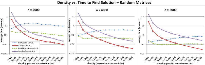
Figure 1 shows the performances of the four implementations on random matrices of several sizes, and varying densities. The matrix densities are similar to those encountered in probabilistic model checking. These graphs indicate that the implementations’ relative performances change their order as the density increases. Furthermore, as the size of the matrix increases, the density at which the performance order changes becomes lower. Thus, which implementation performs best depends on the size and density of the matrix it is being used on.
Generally, the graphs in Figure 1 show that the BiCGStab method is superior to the Jacobi method for denser matrices, but the Jacobi method performs best for very sparse matrices. They also demonstrate a consistent performance benefit from using CUDA to implement the Jacobi method. However, the third graph shows that the CUDA version of the BiCGStab method is only beneficial for larger, denser matrices. For other matrices, the sequential version of the BiCGStab method outperforms the CUDA version.
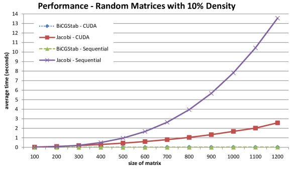
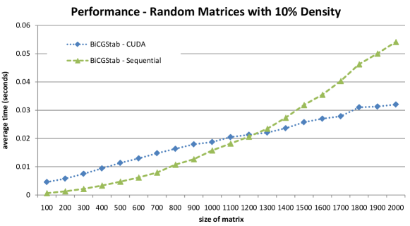
To confirm this, Figure 2 and Figure 3 show the implementations’ performances on random matrices with 10% density. As the sizes of these relatively dense matrices increase, the CUDA versions of both implementations increasingly outperform their sequential counterparts, and the BiCGStab method significantly outperforms the Jacobi method.
7 Performance on Probabilistic Model Checking Data
For these tests, the implementations were tested on matrices representing the transition probability functions of Markov chains based on actual randomized algorithms. These matrices were then reduced to only states and subtracted from the identity matrix, as discussed in Section 2.3.
JPF was used on two randomized algorithms to create this data. The biased die algorithm simulates a biased dice roll by means of biased coin flips, and random quick sort is a randomized version of the quick sort algorithm. Both algorithms were coded in Java by Zhang, who also created the JPF extension that outputs transition probability matrices of Markov chains that correspond to the code being checked [15].
The JPF search strategies used were chosen to create the largest matrices relative to the size of the searched space. JPF’s built-in depth first search was used for random quick sort, and a strategy called probability first search that prioritizes high-probability transitions, also written by Zhang [15], was used for the biased die example.
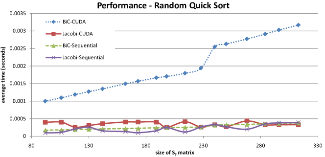
The results of the random quick sort tests are shown in Figure 4, and the results of the biased die tests in Figure 5. Error bars representing standard deviations of each data point are too small to be visible in the graphs. The matrix sizes in the random quick sort tests are much smaller than those in the biased die tests because, while the matrices for random quick sort are initially the same size as or larger than those produced for biased die, much fewer states belong to the set. Furthermore, note that the densities of these matrices decrease as their sizes increase. The sizes and densities of the matrices used in these tests are shown in Table 1.
The relative performances of the sequential and CUDA implementations of the Jacobi method, and the sequential implementation of the BiCGStab method, are different for each algorithm. The best performance on the random quick sort data was from the sequential implementation of the Jacobi method, while the best performance for biased die was from the CUDA implementation of the Jacobi method. The CUDA implementation of the BiCGStab method performs worst in both cases.
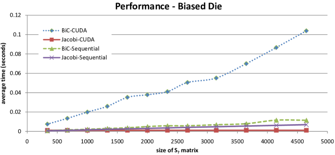
Sizes and Densities of Matrices Random Quick Sort Biased Die density density 92 211 0.025 667 1333 0.003 118 263 0.019 1333 2665 0.001 142 312 0.015 2000 3999 0.001 173 379 0.013 2668 5335 0.001 198 430 0.011 3647 7293 0.001 228 491 0.009 4647 9293 0.000 250 536 0.009 5647 11293 0.000 284 606 0.008 6647 13293 0.000 313 669 0.007 7647 15293 0.000
7.1 Comparing Probabilistic Model Checking Data with Random Matrices
For these tests, random matrices were generated with the same densities and sizes as those produced by JPF (as in Table 1). The JPF matrices are reduced transition probability matrices, subtracted from the identity matrix. So, they have entries in the interval [-1, 1] with locations based on the structure of a Markov chain. In contrast, entries in the randomized matrices are randomly-located positive integers, as described in Section 6. Unlike in the JPF matrix tests, each trial uses a different matrix and vector. However, the standard deviations of the times measured are still too small to be shown on the graphs.
Performance results for these matrices are shown in Figure 6 and Figure 7. It is apparent that the ordering of the different implementations’ performances is the same as it was for matrices of the same sizes and densities generated by JPF. This suggests that size and density are the main determinants of which implementation performs best on probabilistic model checking data, and whether CUDA will be beneficial, rather than other properties unique to the matrices found in probabilistic model checking.
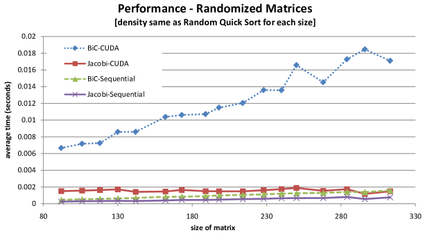
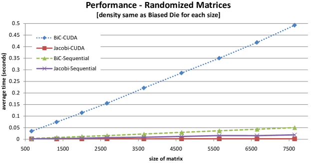
Generally, it appears that for the particular types of matrix encountered during probabilistic model checking, implementing the BiCGStab method in CUDA does not improve performance. CUDA does, however, improve the performance of the Jacobi method.
In [5], the authors conjecture that the Jacobi method would be more suitable for probabilistic model checking using CUDA than Krylov subspace methods such as the BiCGStab method. This seems to be true. However, the results in Section 6 suggest that this is due to the superior performance of the Jacobi method on sparse matrices in general, rather than BiCGStab’s higher memory requirements as proposed in [5]. For the probabilistic model checking data, the matrix density decreases as the size increases, so the conditions in which the CUDA BiCGStab implementation performs best (larger, denser matrices, as in Figure 2) are not encountered.
8 Related and Future Work
Related work by Bosnacki et al. [5] tests a CUDA implementation of the Jacobi method on data obtained by another probabilistic model checker, PRISM. They used different probabilistic algorithms in their probabilistic model checker, and for each algorithm their results show a benefit from GPU usage. In a later expansion of their research [6], they test a CUDA implementation of the Jacobi method that uses a backward segmented scan, and one using two GPUs, which further improve performance. In their second paper they also compare the performance on 32- and 64-bit systems, and find that for one of the three algorithms they model check, the CPU algorithm on the 64-bit system outperforms the CUDA implementation. In another related paper, Barnat et al. [3] improve the performance of the maximal accepting predecessors (MAP) algorithm for LTL model checking by implementing it using CUDA.
Future work could include experiments on model checking data generated from the probabilistic algorithms used with the model checker in [5], to allow closer comparison with that work. Another possibility is to implement the CUDA BiCGStab algorithm using multiple GPUs, so that different steps can be run in parallel.
In [12], Kwiatkowska et al. suggest to consider the strongly connected components of the underlying digraph of the Markov chain in reverse topological order. Since the sizes and densities of the matrices corresponding to these strongly connected components may be quite different from the size and density of the matrix corresponding to the Markov chain, we are interested to see whether this approach will favour different implementations.
Acknowledgements We would like to thank Stefan Edelkamp for providing us their CUDA implementation of the Jacobi method so that we could ensure that our implementation was similar. We also thank the referees for their helpful feedback.
References
- [1]
- [2] Christel Baier & Joost-Pieter Katoen (2008): Principles of Model Checking. The MIT Press.
- [3] Jiri Barnat, Lubos Brim, Milan Ceska & Tomas Lamr (2009): CUDA Accelerated LTL Model Checking. In: Proceedings of the 15th International Conference on Parallel and Distributed Systems, IEEE, pp. 34–41, 10.1109/ICPADS.2009.50.
- [4] Richard Barrett, Michael Berry, Tony F. Chan, James Demmel, June M. Donato, Jack Dongarra, Victor Eijkhout, Roldan Pozo, Charles Romine & Henk Van der Vorst (1994): Templates for the Solution of Linear Systems: Building Blocks for Iterative Methods. SIAM.
- [5] Dragan Bos̆nac̆ki, Stefan Edelkamp & Damian Sulewski (2009): Efficient Probabilistic Model Checking on General Purpose Graphics Processors. In: Proceedings of the 16th SPIN Workshop, Springer-Verlag, pp. 32–49, 10.1007/978-3-642-02652-2_7.
- [6] Dragan Bos̆nac̆ki, Stefan Edelkamp, Damian Sulewski & Anton Wijs (2011): Parallel Probabilistic Model Checking on General Purpose Graphics Processors. International Journal on Software Tools for Technology Transfer 13(1), pp. 21–35, 10.1007/s10009-010-0176-4.
- [7] Peter Buchholz (2006): Structured Analysis Techniques for Large Markov Chains. In: Proceeding of the 2006 Workshop on Tools for Solving Structured Markov Chains, ACM, p. 2, 10.1145/1190366.1190367.
- [8] Abhijeet Gaikwad & Ioane M. Toke (2010): Parallel Iterative Linear Solvers on GPU: A Financial Engineering Case. In: Proceedings of the 18th Euromicro International Conference on Parallel, Distributed and Network-Based Processing, IEEE, pp. 607–614, 10.1109/PDP.2010.55.
- [9] Michael Garland & David B. Kirk (2010): Understanding Throughput-Oriented Architectures. Communications of the ACM 53(11), pp. 58–66, 10.1145/1839676.1839694.
- [10] Boudewijn R. Havertkort (1998): Performance of Computer Communication Systems. John Wiley & Sons.
- [11] David B. Kirk & Wen-mei W. Hwu (2010): Programming Massively Parallel Processors: A Hands-on Approach. Morgan Kaufmann.
- [12] Marta Z. Kwiatkowska, David Parker & Hongyang Qu (2011): Incremental Quantitative Verification for Markov Decision Processes. In: Proceedings of the IEEE/IFIP International Conference on Dependable Systems and Networks, IEEE, pp. 359–370, 10.1109/DSN.2011.5958249.
- [13] Gilbert Strang (2003): Introduction to Linear Algebra. Wellesley-Cambridge Press.
- [14] Henk A. van der Vorst (1992): Bi-CGSTAB: A Fast and Smoothly Converging Variant of Bi-CG for the Solution of Nonsymmetric Linear Systems. SIAM Journal on Scientific and Statistical Computing 13(2), pp. 631–644, 10.1137/0913035.
- [15] Xin Zhang (2010): Measuring Progress of Model Checking Randomized Algorithms. Master’s thesis, York University, Toronto.