Double-resonant fast particle-wave interaction
Abstract
In future fusion devices fast particles must be well confined in order to transfer their energy to the background plasma. Magnetohydrodynamic instabilities like Toroidal Alfvén Eigenmodes or core-localized modes such as Beta Induced Alfvén Eigenmodes and Reversed Shear Alfvén Eigenmodes, both driven by fast particles, can lead to significant losses. This is observed in many ASDEX Upgrade discharges. The present study applies the drift-kinetic Hagis code with the aim of understanding the underlying resonance mechanisms, especially in the presence of multiple modes with different frequencies. Of particular interest is the resonant interaction of particles simultaneously with two different modes, referred to as “double-resonance”. Various mode overlapping scenarios with different profiles are considered. It is found that, depending on the radial mode distance, double-resonance is able to enhance growth rates as well as mode amplitudes significantly. Surprisingly, no radial mode overlap is necessary for this effect. Quite the contrary is found: small radial mode distances can lead to strong nonlinear mode stabilization of a linearly dominant mode.
1 Introduction
Fusion devices contain fast particle populations due to external plasma
heating and (eventually) fusion-borne -particles.
Fast particle populations can interact with global electromagnetic waves,
leading to the growth of MHD-like and kinetic instabilities – e.g., Toroidicity
Induced Eigenmodes (TAE) [1, 2], Reversed Shear
Alfvén Eigenmodes (RSAE) [3]
or Beta Induced Alfvén Eigenmodes (BAE) [4, 5].
In this work, drift-kinetic fast particle simulations performed
with the Hagis code ([6, 7], shortly introduced in section 3) are
carried out to obtain a deeper understanding of
the processes in phase space that occur due to fast particle interaction
with MHD modes. Of interest is the dynamics of wave-fast particle interaction in
scenarios with two modes of different frequencies: what are the mode coupling mechanisms, and
what is the dependence on radial mode distance?
Section 2 gives an overview of the theoretical basis for
these coupling mechanisms.
Section 3 explains in brief, which ASDEX Upgrade reference scenario is selected and
how the MHD equilibrium is processed to give the basis for the Hagis simulations.
In section 4 numerical studies are described, investigating the stochastic threshold and the influence of
on the mode drive. It is found that the presence of a second mode can enhance growth rates as
well as mode amplitudes significantly. As this effect is based on particles that have resonance regions in phase
space with both modes, it is referred to as “double-resonance”. The double-resonant effect was expected
to decrease with the radial mode distance, but it turned out, that the picture is more complicated.
2 Theoretical Picture of Double-Resonance
Theory (e.g. Ref. [8]) predicts that conversion of free energy
to wave energy is enhanced in a multiple-mode scenario, i.e., the interaction of multiple modes produces
energy conversion rates higher than that which would be achieved with each mode acting independently.
This can be partially explained by the principle of gradient (of the radial particle distribution) driven
mode growth – according to111Throughout this work, refers to the radial coordinate as
the square root of the normalized poloidal flux:
.
[9] – which can be extended to
multiple modes [10, 11, 12, 8].
This picture of gradient driven double-resonance is based on the
precondition that modes share resonances in the same phase space area.
Through the resulting redistribution by each mode, a steeper gradient
is produced at the other mode’s position, enhancing its drive. The
overlapping of modes leads then to a much larger conversion of free energy to wave
energy.
However, this mechanism can only work if there is also spatial mode overlap in
the radial direction. In Ref. [13] simulations were carried
out, finding a double-resonant effect also without this precondition.
Furthermore, a superimposed oscillation on the modes’ amplitudes was observed,
clearly indicating mode-mode interaction. The modes without radial overlap
are then coupled radially through the particles’ trajectories: A population
of particles that shares resonances in phase space with both modes and passes
both modes’ location at once, can transfer energy from one mode to the other [13].
Since the particle orbits are characterized by a certain width, it is not necessary that
both modes have a radial overlap.
In the following, this mechanism is called inter-mode energy transfer:
By damping one mode, particles gain energy and also toroidal momentum
due to [7]
| (1) |
As Alfvénic mode frequencies are very low (compared to the particles’ cyclotron frequency), momentum transfer dominates over energy transfer. Since , particles gaining energy from the wave (i.e. damping it), are redistributed radially inwards, whereas particles losing energy to the wave (i.e. driving it), are redistributed radially outwards. The latter is the dominant process and is caused by the negative slope of the particles’ radial distribution function. When passing through the second mode, the particles lose energy and toroidal momentum by driving the mode. As there is no radial net drift in this mechanism, it can continue as long as the dominant mode is strong, making this the dominant process over other possible combinations of mode-mode energy exchange. Particles that gain energy from both modes or lose energy to both modes soon leave the resonant phase space area. It is the exchange of energy between the modes that leads to the observed oscillation of their amplitudes: The mode receives energy in the rhythm of the particles’ bounce frequency , which equals the beat frequency of both modes as shown in the following: Trapped particles with a bounce frequency and toroidal precession frequency interact with MHD modes of a certain frequency , if the resonance condition [14]
| (2) |
is fulfilled, where is the toroidal mode harmonic and the particles’ bounce harmonic. For double-resonance, this resonance condition has to be fulfilled for both modes ’1’ and ’2’ simultaneously, leading to
| (3) |
For the simplest case, the toroidal mode numbers are considered equal, and , . This leads to . Indeed, the lowest bounce harmonics are the most relevant ones; however, the issue of different toroidal mode numbers will be discussed later.
3 Using the Hagis Code with an ASDEX Upgrade Plasma Equilibrium
The numerical investigations presented in this work are performed with
the Hagis Code [6, 7],
a nonlinear, drift-kinetic, perturbative Particle-in-Cell code (current release 12.05).
Hagis models the interaction between a distribution of energetic particles and a set
of Alfvén Eigenmodes. It calculates the linear growth rates as well as the nonlinear behavior
of the mode amplitudes and the fast ion distribution function that are determined by
kinetic wave-particle nonlinearities. It is fully
updated to work with MHD equilibria given by the recent Helena [15] version.
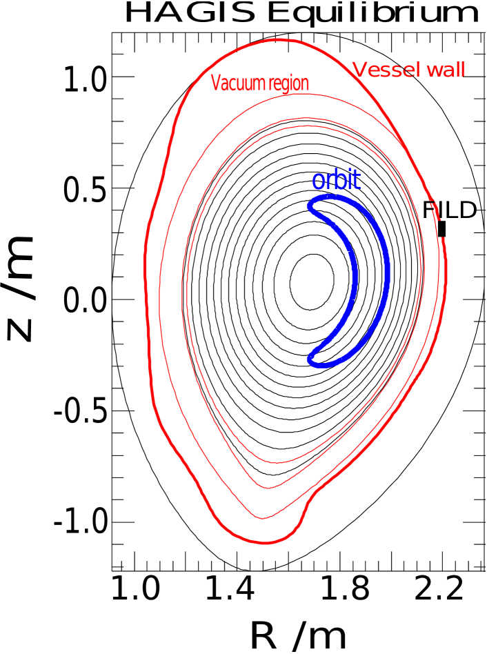 Figure 1: Hagis equilibrium with vacuum region (red),
representative banana orbit (blue) and FILD position (black square).
Figure 1: Hagis equilibrium with vacuum region (red),
representative banana orbit (blue) and FILD position (black square).
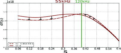
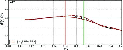
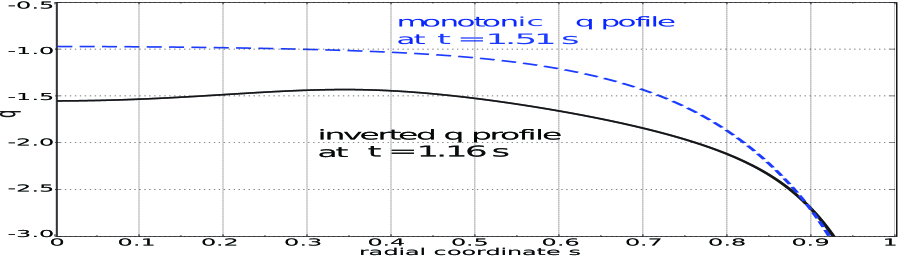 Figure 2: profile according to experimental measurements in
AUG discharge #23824 at different time
points: s (black solid line) and s (blue dashed line):
the profiles differ in the shape (the earlier one is inverted, the later one monotonic), but
also in the absolute values (the inverted profile has higher absolute values).
The plasma equilibrium (figure 1) for Hagis is based
on the Cliste code [16, 17],
then transformed via Helena to straight field line coordinates and
to Boozer coordinates by Hagis.
Figure 2: profile according to experimental measurements in
AUG discharge #23824 at different time
points: s (black solid line) and s (blue dashed line):
the profiles differ in the shape (the earlier one is inverted, the later one monotonic), but
also in the absolute values (the inverted profile has higher absolute values).
The plasma equilibrium (figure 1) for Hagis is based
on the Cliste code [16, 17],
then transformed via Helena to straight field line coordinates and
to Boozer coordinates by Hagis.
The data for the MHD equilibria of all simulations presented in the following originate from the
ICRH minority heated ASDEX Upgrade (AUG) discharge #23824, at time s
or s.
At the earlier time point, the profile is slightly inverted (figure 2, black solid line),
whereas at the later time point, it is monotonic, with lower absolute values (figure 2,
blue dashed line).
The plasma equilibrium, and in particular the profile is determined by Alfvén spectroscopy of
the RSAEs:
magnetic pick-up coil data and soft X-ray emission measurements are used to determine the
profile’s minimum value and location.
This particular discharge was chosen due to the availability of especially detailed
experimental data concerning fast particle-mode interaction. However, a detailed comparison between
numerical and experimental results goes beyond the scope of this work, but is the
object of current and future
investigation. In this work, a numerical study is presented, that is based on an AUG reference case:
the profile as well as the mode frequencies, harmonics and widths are chosen according to
experimental observation. However, significant abstractions have also been made:
the mode structures are chosen analytically, as well
as the particle distribution functions. Furthermore, mode saturation is based completely on
the depletion of the particle distribution function, no collisions, nor turbulence are taken
into account, and there is no source term for energetic particles.
4 Numerical Study on Double Mode Resonance
In this section, a numerical study is presented that examines under which circumstances mode-particle interaction can take place. A special focus is set on the interaction with multiple modes of different frequencies.
4.1 Simulation Conditions
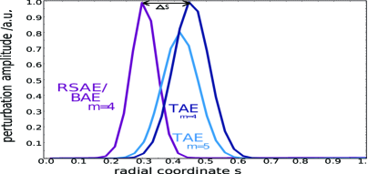
As the question of understanding double mode resonance is very fundamental, the simulations were performed under quite simple, but still realistic physical conditions: the volume averaged fast particle beta is chosen to be . To avoid different mode drive at different radial mode positions only due to a steeper gradient in the distribution function, a radial particle distribution with constant gradient is chosen. As energy distribution function a slowing down function [18] is used:
| (4) |
( MeV, MeV, MeV). The particles are distributed isotropically in pitch angle (as e.g., fusion-borne particles would be). As MHD perturbations, analytic, gauss shaped functions are used (see figure 3), without background damping. The mode frequencies are chosen to match experimental data: at both time points within the considered discharge #23824, a high frequency TAE with kHz is found, as well as a lower frequency mode at kHz. Ref. [19] describes their mode as a RSAE at s and as BAE at s. The widths of the modes are based on the MHD eigenfunctions, calculated numerically with the linear eigenvalue solver Ligka [20].
Convergence tests indicate that simulations with 120000 markers are sufficient, leading to computational costs of a few hundred CPUh for each simulation.
4.2 Simulation Results
Multi-mode simulations are carried out with different radial distances between the Alfvénic modes. It is helpful to look at the different stages within the simulation individually: although all simulations are performed including all nonlinearities, the nonlinear effects are small at the beginning of each simulation, leading to an amplitude growing according to with the so-called linear growth rate.
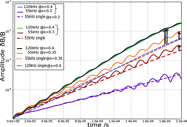
The linear regime
The modes’ amplitudes in this linear regime, as depicted in
figure 4
confirm already some of the results presented in [13]:
at least one mode grows faster in the double mode scenario compared
to the single mode simulation (the TAEs in figure 4
dark colors).
In most cases, both modes have larger growth rates in the double mode scenario than
in the single mode simulation. Furthermore, it is usually the radially outer mode that
is driven most strongly due to the double mode resonance.
This is because gradient driven double-resonance is most effective in
driving the outer mode: through resonant particle redistribution, one mode produces steeper
gradients at the other mode’s position. Through the inner mode, particles are
redistributed towards the outer position and supply it with more (resonant) particles,
that can transfer their energy to the wave. At the inner mode’s position, in contrast,
the particle population decreases, and with it, the energy transfer to the wave.
However, in simulations with low growth rates
(see linear phase of figure 10),
the stronger – and that is mostly the outer mode – was enhanced
in mode drive less effectively than the subdominant one, or even weakened
compared to the single mode case. In these cases, the inter-mode energy exchange
is the prevailing mechanism, conducting energy from the stronger
to the weaker mode.
A superimposed oscillation is visible, strongest if the
modes’ growth rates are relatively
different from each other. However, if they differ too much,
the oscillation becomes jagged, due to
the large impact of the dominant mode on the subdominant one.
The oscillation frequency matches the beat frequency of both
modes kHz,
a hint for working inter-mode energy transfer.
As stated in Ref. [13], both mode numbers have to be equal to lead
to the oscillatory behavior, i.e. to double mode resonance, as
will be discussed later.
In the course of each simulation, nonlinear effects become more and more important,
leading to a mode amplitude evolution different from .
The beginning of the nonlinear regime is observed, when the mode amplitude changes
from evolving linearly (in a semilogarithmic plot) to saturating at a certain level.
The nonlinear regime
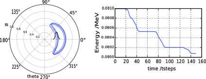
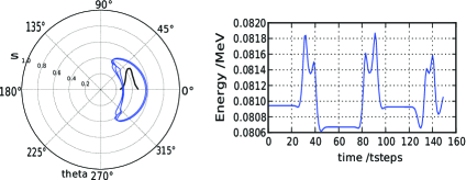
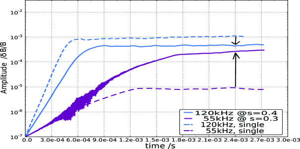
The effect of the double-resonance in the nonlinear regime is clearly visible in figure 5 ():
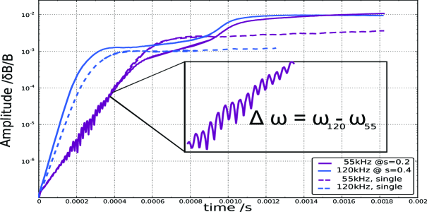
in the double mode scenario, the modes not only grow faster (in the case of the TAE), but also saturate at a higher level compared to the single mode case (by about a factor of five to ten). This is due to the orbit stochasticization at already discovered in single mode simulations: The stochastic threshold [8] is only reached in the double mode scenario, not in the single mode case. To visualize the effect of stochasticization, an representative particle orbit and the particle’s energy evolution before and after the stochasticization sets in is shown in figure 6.
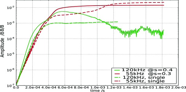
The picture is not as simple in the second example considered
(, figure 7):
at the beginning of the nonlinear regime,
double-resonance is effective – mode amplitudes are higher by a factor of five compared
to the single mode simulation. At a later time point in the simulation
however, the situation changes
completely: the TAE amplitude vanishes and the RSAE saturates at a lower level compared to
the amplitude it reached in the single mode scenario during stochasticization. This scenario
was found frequently for close radial mode distances, and shows that a linearly dominant
mode can be stabilized nonlinearly in a multi-mode scenario.
The reason for this behavior can be found in the radial particle redistribution. To find out the redistribution caused solely by the RSAE, the single mode simulation of that mode has to be considered: the RSAE leads to a radial particle redistribution as depicted in figure 8a). This redistribution leads to a flattened gradient (figure 8b) at , the position of the TAE in the the double mode case of figure 7. The reason for the destruction of the TAE in this simulation is therefore its radial location too close to the RSAE. However, at all positions , the gradient becomes steeper in the course of the single mode simulation. Indeed, simulating the RSAE with a TAE in this radial range leads to strong TAE drive.
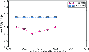
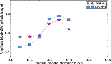
A scan over the radial mode distance reveals an effective double-resonance as shown in
figure 9: depicted are the ratios of the linear growth rates (a) and the amplitudes
(b) in the double mode case vs. the single
mode case over the radial mode distance .
The amplitude level was compared after TAE periods ( ms) of
simulated time. This time is sufficient for the single amplitudes to saturate,
but still significantly below energy slowing down time. Therefore, the fact that
no source term is implemented in the code does not disturb the physical picture.
One can see that the growth rates of
both the TAE and the RSAE are enhanced in all double mode cases compared to the single mode ones.
However, the growth rate of the outer TAE is enhanced most strongly and independently
of the radial
mode distance – i.e. gradient driven double-resonance works even if there is no radial mode overlap.
In contrast, the enhancement of the inner and weaker RSAE decreases with the radial
mode distance for small . Then it increases again for .
These larger mode distances match the double-resonant
particle orbits and therefore enable inter-mode energy exchange, driving the weak mode. For
higher , the larger, i.e. higher energetic orbits fit the mode distance
and lead to even more energy exchange.
Furthermore, with larger radial mode distances, the modes are able to tap energy from a wider
gradient region. The amplitude ratios, however, are even lowered in the double-resonant case
compared to the respective single mode levels, if the radial mode distance is small. This happens
due to the mutual gradient depletion at the
other mode’s radial position. If the modes feature a larger radial distance (), the
double mode scenario amplitudes are much higher compared to the single mode amplitudes, both for the
TAE and the RSAE. Both modes benefit from each other – most for a radial distance of about
.
It is important to note that the distance giving maximum amplitude ratios depends
strongly on the absolute mode positions with respect to the radial distribution function,
and especially on the amplitude regime (stochastic or non-stochastic) of each mode.
The same applies for the value at which the transition towards
double-resonant amplitude enhancement takes place.
To summarize, one can say, that growth rates are
generally enhanced by the presence of another mode, whereas for the amplitudes, this is only
the case, if the modes feature a sufficient radial distance. For small distances, modes at radial
positions, where the initial distribution function is already relatively flat, double-resonance
leads to strong mode stabilization. If the amplitudes are enhanced, their amplification level is,
however, mainly determined by whether the mode reaches the stochastic regime.
The probability of reaching the stochastic threshold rises strongly if a second mode is present.
However, if the growth rates are relatively low for some reason (e.g. small mode width, small fast particle beta), the particle redistribution is not strong enough to lead to a dominant gradient driven double-resonance. In these cases, the inter-mode energy transfer mechanism can prevail (even in a later phase). The dominant mode is weakened through inter-mode energy transfer to the subdominant mode, as depicted in figure 10. The process saturates, as the modes’ amplitudes converge towards comparable levels. In this simulation, there is no strong fast particle redistribution.
In the monotonic profile equilibrium (shown in figure 2), the Alfvénic modes as simulated within this study do not grow up to the stochastic regime. In order to also be able to investigate the stochastic phase in the monotonic profile case, one can shift the modes further outward radially, where the mode drive is higher. Such simulations revealed interesting possibilities for interplay between the two double-resonance mechanisms: e.g., it is possible that the mode in the flattened-gradient region is not weakened, but rather the other mode. In this scenario the mode at the position of the flattened gradient is driven solely through energy transfer from the other mode, as there is no gradient-caused mode drive remaining. Eventually, this leads to a depletion of the other (stronger) mode’s amplitude.
4.2.1 The role of trapped particles
Another question regards the role of trapped particles in the double-resonance mechanisms:
Especially for the inter-mode energy exchange, the particles’ orbit
widths are crucial. Therefore, the
question arises if the major part of the double-resonance is carried
by the trapped particle population or by the passing particles.
In Hagis it is possible not to load any trapped particles at all. In
the simulations presented in the following,
the code was modified to even neglect particles that become trapped
in the course of the simulation.
It was found that for the linear phase, the absence of trapped particles
leads to significantly lower growth rates. This effect is slightly stronger
for inner mode positions, although there would be more trapped particles further
outside. This is due to the fact that the orbit width broadens with radial position,
and therefore also the loss region. But especially the resonance with a broader TAE
is effective only with broader orbit particles that are more easily lost.
However, except for the effect of generally lower amplitudes in the scenario without trapped particles,
the double-resonance also works with passing particles alone:
the effect of double-resonance
remains, which is reflected by the ratio of growth rates and amplitude levels in double mode simulations
over those from single mode simulations. This means, passing as well as banana orbits
can be adequate orbits for the double-resonance mechanism of inter-mode energy transfer:
As for passing particles, the orbit does not close entirely on the low field side,
the double-resonance mechanism must work with the higher poloidal harmonics of one mode,
located at the high field side. For the TAE, due to strong ballooning effects, there are no
significant maxima at the high field side. Core-localized modes, such as
BAE and RSAE do not couple to the next harmonic and are cylindrical modes that
feature higher harmonics at the high field side. There, double-resonant passing particles
can transit the mode. Compared to the banana width of a trapped particle, the
drift displacement of a passing particle’s orbit (at the same energy) is
significantly smaller. But, as the resonance condition is different for passing particles,
higher energetic particles are responsible for double-resonance. These feature a larger
drift displacement, that fits again the simulated radial mode distances .
However, for the gradient driven (double as well as single) resonance, the trapped particles’
resonances are very important. It was not possible to quantify this further.
Without trapped particles, the saturation levels are much lower and do not reach the stochastic regime.
This is due to the importance of the trapped particles’ (single) resonances, leading to gradient driven
mode-particle interaction. The importance of the trapped particles is consistent
with the fact, that the TAE is an even TAE, which is known to interact very strongly with trapped particles.
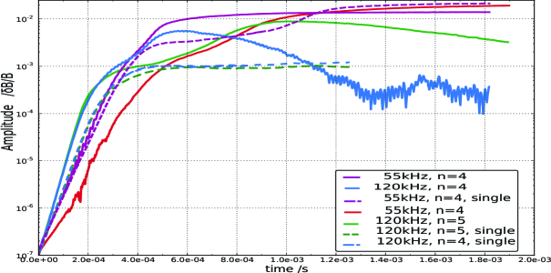
4.2.2 The importance of equal toroidal mode numbers
Especially for the inter-mode energy transfer, there has to be a population of particles that is resonant with both modes at once. For two modes with different toroidal mode numbers , the overlapping volume of resonances in phase space becomes smaller, and it becomes less probable to find particles that fulfill the resonance condition eq. (3) for two modes at once, and it is expected that less double mode resonance effects occur, if the modes differ in their toroidal mode number . Figure 11 shows the resulting amplitude evolution in a double mode simulation with different for the RSAE () and TAE (). In the linear phase, one can see clearly that the amplitudes of the single TAE simulations are almost exactly equal, independent on . However, in the double mode scenario, the RSAE is enhanced (compared to the single mode amplitude), and the TAE even more strongly – but only if both modes have equal . If this is not the case, only the TAE is enhanced, whereas the RSAE actually decreases. Furthermore, the superimposed oscillation vanishes to a slightly jagged curve. This shows that gradient driven double-resonance still works with different toroidal – the outer mode amplitude is still enhanced – but the inter-mode energy transfer mechanism breaks down, as the resonance condition cannot be easily fulfilled for both modes at once for particles with trajectories through both modes: the inner RSAE amplitude is not enhanced, but weakened. When reaching saturation, the effect of inter-mode energy transfer is overlapped by the dominance of the gradient driven double-resonance, and therefore, the saturation levels do not depend strongly on equal . Simulations with different show almost identical nonlinear behavior, although saturation is reached later. The stochastic threshold does not seem to be influenced by the differing , nor the effect that one mode can be damped by the redistribution of the other one. However, the differences again depend on the exact scenario.
5 Conclusions
The interaction of fast particles with Alfvén Eigenmodes of different frequencies was
studied numerically with the Hagis Code
in a simple, but physically realistic picture for two different MHD equilibria occurring
during the ASDEX Upgrade discharge #23824.
Double-resonant mode drive was compared to single mode scenarios, verifying previous
findings of double-resonance mechanisms:
gradient driven double-resonance [8] and inter-mode energy transfer [13].
The latter was observed to prevail only in low amplitude cases,
enhancing the weaker mode at the expense of the dominant one.
A superimposed beat frequency oscillation on both modes’ amplitudes was found,
as well as higher linear growth rates – at least for one mode – compared to the single mode
reference cases.
The growth rate enhancement was observed to have only a very weak dependence
on the radial mode distance.
Concerning the amplitudes of the Alfvén Eigenmodes,
double-resonance can enhance modes into the stochastic regime and therefore lead to much higher
saturation levels compared to the single mode scenarios, even if there
is no radial mode overlap.
However, close radial mode distances were found to destroy
linearly dominant modes when the nonlinear regime sets in.
As a consequence, linearly weaker modes may become nonlinearly dominant.
These results reveal a complex nonlinear evolution of multi-mode scenarios, rather
than merely a simple continuation of the linear multi-mode behavior.
The authors wish to thank D.R. Hatch for proof reading.
References
- [1] Cheng C Z, Chen L and Chance M 1985 Ann. Phys. 161 21 – 47
- [2] Cheng C Z and Chance M S 1986 Phys. Fluids 29 3695–3701
- [3] Berk H L, Borba D N, Breizman B N, Pinches S D and Sharapov S E 2001 Phys. Rev. Lett. 87
- [4] Heidbrink W W, Strait E J, Chu M S and Turnbull A D 1993 Phys. Rev. Lett. 71(6) 855–858
- [5] Turnbull A D, Strait E J, Heidbrink W W, Chu M S, Duong H H, Greene J M, Lao L L, Taylor T S and Thompson S J 1993 Phys. Fluids B 5 2546–2553
- [6] Pinches S D et al 1998 Comput. Phys. Commun. 111
- [7] Pinches S D 1996 Nonlinear Interaction of Fast Particles with Alfvén Waves in Tokamaks Ph.D. thesis University of Nottingham
- [8] Berk H L, Breizman B and Ye H 1992 Phys. Rev. Lett. 68(24)
- [9] Fu G Y and Dam J W V 1989 Phys. Fluids B 1
- [10] Berk H L and Breizman B N 1990 Phys. Fluids B 2 2226–2234
- [11] Berk H L and Breizman B N 1990 Phys. Fluids B 2 2235–2245
- [12] Berk H L and Breizman B N 1990 Phys. Fluids B 2 2246–2252
- [13] Brüdgam M 2010 Ph.D. thesis Technische Universität München
- [14] Porcelli F, Stankiewicz R, Kerner W and Berk H L 1994 Phys. Plasmas 1
- [15] Huysmans G T A et al 1990 Conf. on Computational Physics Proc. World Scientific, Singapore (AIP)
- [16] Mc Carthy P J 1999 Phys. Plasmas 6 3554–3560
- [17] Mc Carthy P J and the ASDEX Upgrade Team 2012 Plasma Phys. Control. Fusion 54 015010
- [18] Gaffey J D 1976 J. Plasma Phys. 16 149–169
- [19] Lauber Ph et al 2009 Plasma Phys. Control. Fusion 51
- [20] Lauber Ph, Günter S, Könies A and Pinches S D 2007 J. Comp. Phys. 226 447 – 465