CERN-PH-TH/2012-040

HIP-2012-06/TH

NSF-KITP-12-017

YITP-12-7

Numerical properties of staggered quarks
with a taste-dependent mass term

Philippe de Forcrand,^a,b,c,d Aleksi Kurkela^e and Marco Panero^c,f

^a Institute for Theoretical Physics, ETH Zürich, CH-8093 Zürich, Switzerland

^b CERN, Physics Department, TH Unit, CH-1211 Genève 23, Switzerland

^c Kavli Institute for Theoretical Physics, University of California, Santa Barbara, CA 93106, USA

^d Yukawa Institute for Theoretical Physics, Kyoto University, Kyoto 606-8502, Japan

^e Department of Physics, McGill University, 3600 rue University, Montréal, QC H3A 2T8, Canada

^f Department of Physics and Helsinki Institute of Physics, University of Helsinki, FIN-00014 Helsinki, Finland

e-mail:       forcrand@phys.ethz.ch, aleksi.kurkela@mcgill.ca, marco.panero@helsinki.fi

The numerical properties of staggered Dirac operators with a taste-dependent mass term proposed by Adams [1, 2] and by Hoelbling [3] are compared with those of ordinary staggered and Wilson Dirac operators. In the free limit and on (quenched) interacting configurations, we consider their topological properties, their spectrum, and the resulting pion mass. Although we also consider the spectral structure, topological properties, locality, and computational cost of an overlap operator with a staggered kernel, we call attention to the possibility of using the Adams and Hoelbling operators without the overlap construction. In particular, the Hoelbling operator could be used to simulate two degenerate flavors without additive mass renormalization, and thus without fine-tuning in the chiral limit.

1 Introduction

The spontaneous breakdown of chiral symmetry plays a central role in the spectrum of light hadrons. Since it is an intrinsically non-perturbative phenomenon, the only way to study it from the first principles of QCD is via the lattice regularization. Yet, already many years ago Nielsen and Ninomiya proved that a translationally invariant, local lattice formulation of the QCD Dirac operator $D$, retaining chiral symmetry in the massless limit, and with the correct number of physical fermionic degrees of freedom, is forbidden [4]. This no-go theorem can be circumvented, by constructing lattice fermions satisfying a modified form of chiral symmetry [5], and obeying the Ginsparg- Wilson relation [6]. Although explicit formulations of lattice Ginsparg-Wilson fermions are known [7], currently their practical use in realistic, large-scale lattice QCD simulations is still limited, due to the high computational overhead.

The most widely-used lattice discretizations of the Dirac operator are either based on the addition of a second-derivative term to the kinetic part of the quark action [8] to remove (or “quench”) the unphysical “doubler” modes in the continuum limit by giving them a mass ${\cal O}(a^{-1})$, or on a site-dependent spin diagonalization, which leads to the so-called staggered formulation [9]. The former approach introduces an explicit breaking of chiral symmetry, and, as a consequence, an additive renormalization of the quark mass, which has to be fine-tuned. In contrast, the staggered operator preserves a remnant of chiral symmetry (sufficient to forbid additive mass renormalization), and leads to a reduction of the matrix size. However, the staggered formulation only removes part of the unphysical modes, reducing the number of quark species in four ($d$) spacetime dimensions from 16 ($2^{d}$) down to four ($2^{d/2}$) “tastes”, which become degenerate [10] (and consistent with the properties related to the global symmetries of the continuum Dirac operator [11]) in the $a\to 0$ limit. In order to simulate QCD with two light fermions, one then has to apply the so-called “rooting trick”, which has been a subject of debate for the last few years [12].

Some recent works have discussed the idea of using a staggered kernel with a taste-dependent mass term to obtain two (or one [13, 3]) massless fermion species. Such formulation, which is one of the various approaches aiming at minimally doubled fermions [14], could combine the advantages of the overlap construction with the computational efficiency of a staggered kernel. Furthermore, this formulation appears to be particularly attractive from the point of view of topological properties [1].

Using a staggered operator with a “flavored” mass term as the kernel in an overlap construction is a very appealing idea, but the properties of such operators (with various taste-dependent mass terms) are interesting on their own. In fact, while the overlap construction completely removes the need for fine tuning to achieve massless fermions, it still leads to a considerable computational overhead. In contrast, using a staggered operator with taste-dependent mass à la Wilson requires fine tuning to obtain exactly massless modes, but, by virtue of the reduced size of the operator, may still be a computationally competitive alternative to the usual Wilson discretization, while avoiding the rooting prescription.

This motivation led us to address a numerical investigation of different operators of this type that we present here (preliminary results have appeared in [13]). In the following, we present a systematic classification of the possible taste-dependent mass terms, discuss their analytical features in the free theory, and then move on to the interacting case that we study via numerical simulations. We perform an elementary measurement of the pion mass on a set of quenched configurations, and verify the expected PCAC behaviour as one approaches the chiral limit. In an Appendix, we also explore the properties of the staggered overlap operator proposed in [1], in comparison with the usual overlap based on the Wilson kernel. In particular, we compare the locality of the operators, and the computational cost of applying them to a vector and of solving for the quark propagator.

The structure of this paper is as follows. First, in sec. 2 we recall theoretical aspects of the construction of taste-dependent mass terms, and discuss their spectral structure in the free field case. Then, we address the interacting case, presenting our numerical studies in sec. 3. We summarize our findings and discuss their implications for possible future, large-scale applications of these operators in sec. 4. Finally, in the appendix A, we report on our study of an overlap operator based on a staggered kernel, as proposed in ref. [1].

2 Theoretical formulation and general features

The staggered operator [9]

$$D_{\text{KS}}=\frac{1}{2a}\sum_{\mu=1}^{d}\eta_{\mu}\left(V_{\mu}-V_{\mu}^{\dagger}\right)$$ (1)

with $\eta_{\mu}(x)=(-1)^{\sum_{\nu<\mu}x_{\nu}}$ and $\left(V_{\mu}\right)_{x,y}=U_{\mu}(x)\delta_{x+a\hat{\mu},y}$, is a computationally very efficient way to discretize the massless QCD Dirac operator on a $d$-dimensional Euclidean hypercubic lattice of spacing $a$. This operator is invariant under a global $U(1)$ symmetry, which can be interpreted as a remnant of chiral symmetry: in fact, $D_{\text{KS}}$ anticommutes with the operator $\Gamma_{55}$ defined by $\left(\Gamma_{55}\right)_{x,y}=(-1)^{\sum_{\nu=1}^{d}x_{\nu}}$. In the free theory, one can easily see that in four dimensions the operator $\Gamma_{55}$ has $\gamma_{5}\otimes\gamma_{5}$ structure in spin-taste space [16]. The construction of $D_{\text{KS}}$ is based on a local spin diagonalization, which, for the four-dimensional case, allows one to reduce the number of fermion components by a factor of $4$ with respect to the naive operator, and yields four tastes in the continuum limit. The degeneracy between these four tastes is explicitly broken by gauge interactions at finite lattice spacing $a$, but is recovered in the continuum limit $a\to 0$.

Recently, various works explored the idea of using staggered operators with taste-dependent mass terms [1, 13, 3]. Following, e.g., the discussion in the classic paper by Golterman and Smit [17], the possible matrix structures (in taste space) for a mass term can be classified as

• $\mathbf{1}$ (“0-link”), of the form $\delta_{x,y}$

• $\gamma_{\alpha}$ (“1-link”), involving a sum of terms, each containing 1 link $U_{\mu}$

• $\sigma_{\alpha\beta}$ (“2-link”), involving a sum of terms, each containing 2 links $U_{\mu}U_{\nu}$

• $\gamma_{5}\gamma_{\alpha}$ (“3-link”), involving a sum of terms, each containing 3 links $U_{\mu}U_{\nu}U_{\rho}$

• $\gamma_{5}$ (“4-link”), involving a sum of terms, each containing 4 links $U_{\mu}U_{\nu}U_{\rho}U_{\sigma}$

It is highly desirable to preserve the symmetry $\Gamma_{55}D\Gamma_{55}=D^{\dagger}$, because it guarantees that $\det D$ is real, and non-negative (in the absence of real negative eigenvalues), thus avoiding a “sign problem” in the measure [18]. This symmetry is satisfied only if the hermitian mass term connects sites of the same parity. Thus, we do not consider the 1-link or a 3-link mass terms further.

This leaves three possibilities: 0-, 2- and 4-link mass terms. The 0-link mass term corresponds to the usual staggered operator, with a taste-independent bare mass

$$D_{0}=D_{\text{KS}}+m.$$ (2)

The staggered operator with a 2-link mass term, which was discussed in refs. [13, 3], can be written in the form

$$D_{2}=D_{\text{KS}}+\frac{\rho}{\sqrt{3}}\left(M_{12}+M_{13}+M_{14}+M_{23}-M_{24}+M_{34}\right),$$ (3)

where (following the notation of ref. [3])

$$M_{\mu\nu}=i\eta_{\mu\nu}C_{\mu\nu},$$ (4)

$$(\eta_{\mu\nu})_{x,y}=-(\eta_{\nu\mu})_{x,y}=(-1)^{\sum_{i=\mu+1}^{\nu}x_{i}}\delta_{x,y}\textrm{, for $\mu<\nu$},$$ (5)

$$C_{\mu\nu}=\frac{1}{2}\left(C_{\mu}C_{\nu}+C_{\nu}C_{\mu}\right),$$ (6)

$$C_{\mu}=\frac{1}{2}\left(V_{\mu}+V_{\mu}^{\dagger}\right).$$ (7)

Finally, a staggered operator featuring a mass term with $\gamma_{5}$ structure in taste space [1] can be written as

$$D_{4}=D_{\text{KS}}-\frac{\rho}{a}\Gamma_{55}\Gamma_{5},$$ (8)

with

$$\Gamma_{5}=\eta_{5}C,$$ (9)

where

$$\eta_{5}(x)=\prod_{\mu=1}^{4}\eta_{\mu}(x),$$ (10)

while $C$ is the average of four-link parallel transporters joining sites at opposite corners of the elementary lattice hypercubes

$$C=\frac{1}{4!}\sum_{\mbox{\tiny{perm}}}C_{\mu}C_{\nu}C_{\rho}C_{\sigma}.$$ (11)

Note that the mass term appearing on the r.h.s. of eq. (8) is Hermitean and commutes with $\Gamma_{55}$.

     

Figure 1: Left panel: Spectrum of $D_{\text{KS}}$ in the free limit. Central panel: Free spectrum of operator $D_{2}$ (eq.(3)), which includes a taste-dependent mass term with tensor-like structure in taste space (i.e., a 2-link mass term). Right panel: Free spectrum of operator $D_{4}$ (eq.(8)), which includes a taste-dependent mass term with $\gamma_{5}$ structure in taste space (i.e., a 4-link mass term).

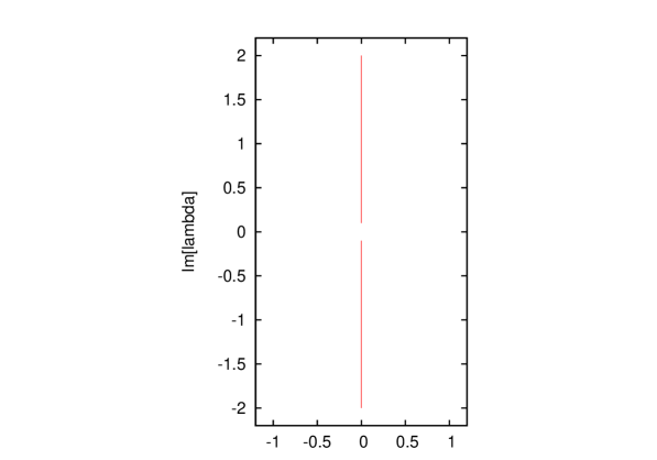
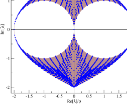
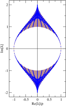
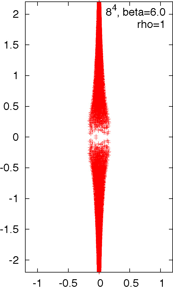
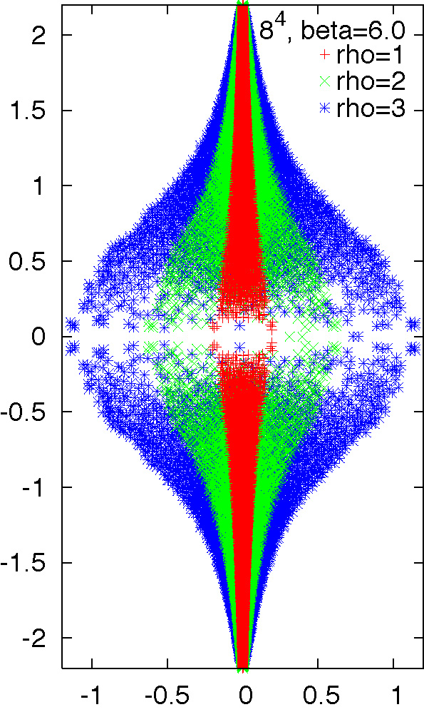
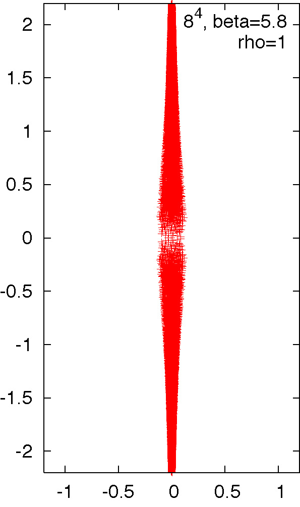
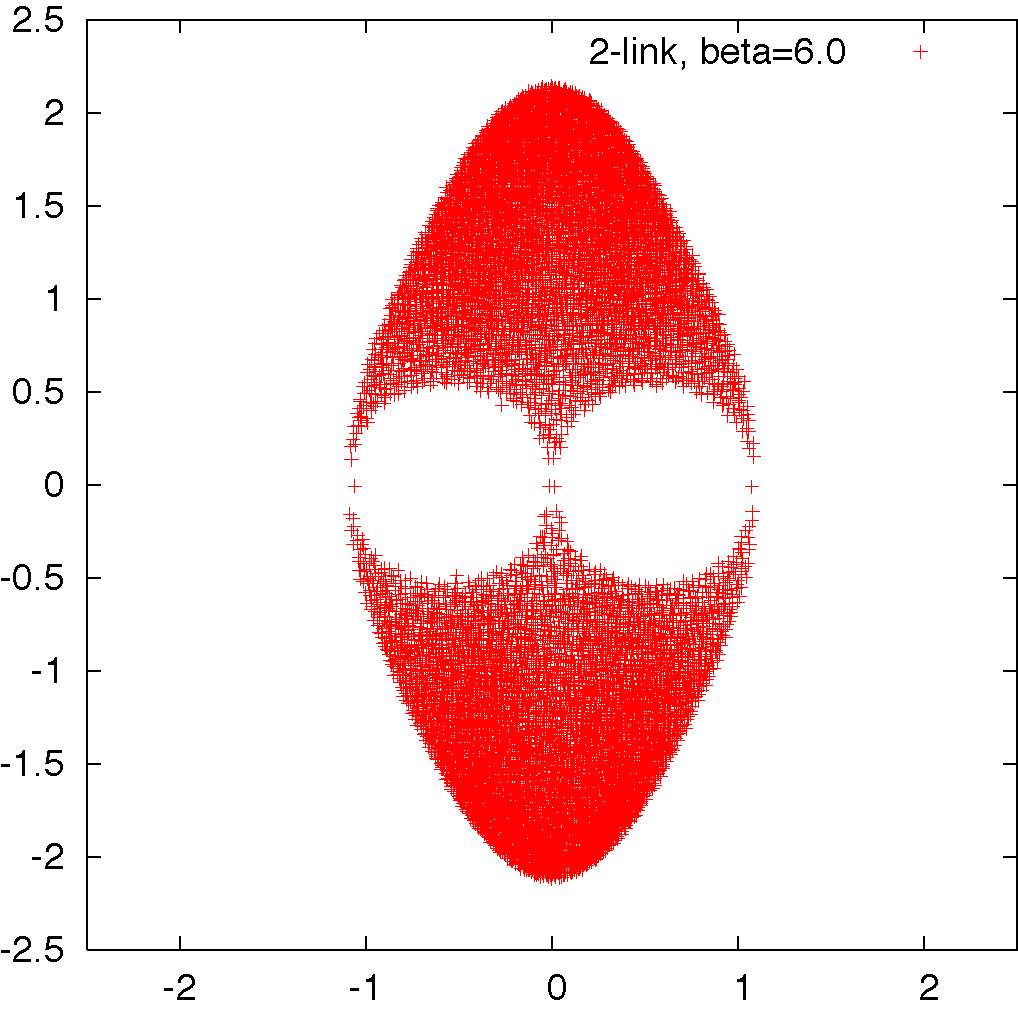
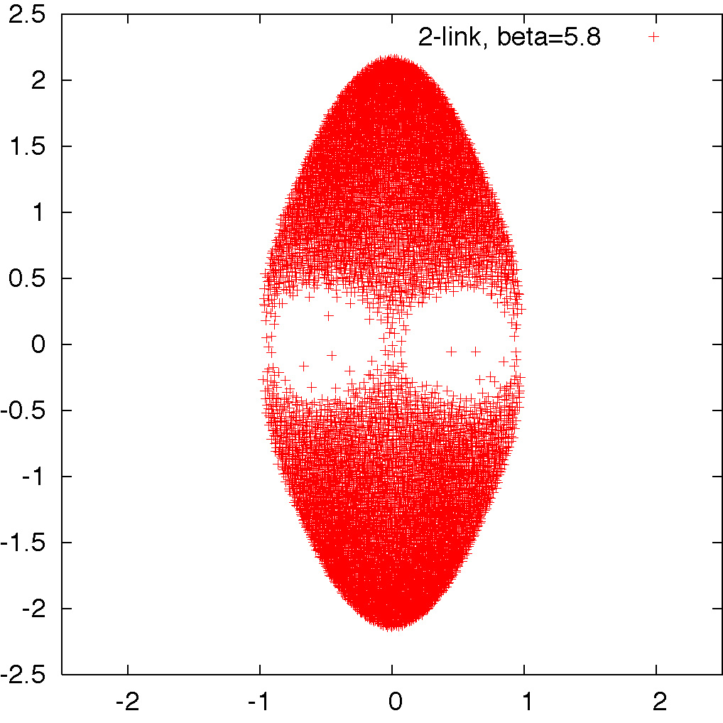
To understand the properties of these three different types of operators it is instructive to start by discussing their spectra in the free limit. The three panels in Fig. 1 show the structure of the spectrum of eigenvalues for $D_{\text{KS}}$ (for $D_{0}$, the spectrum is just trivially shifted by $m$), for $D_{2}$, and for $D_{4}$ in the non-interacting case.

In the free limit the eigenvalues of $D_{0}$ on a lattice with $N_{\mu}$ sites along the $\mu$ direction read

$$\lambda=m\pm i\sqrt{\sum_{i=1}^{d}\sin^{2}p_{\mu}},\qquad\mbox{with: }\;\;p_{\mu}=\frac{2\pi}{N_{\mu}}(k_{\mu}+\varepsilon_{\mu}),\qquad k_{\mu}\in\{0,1,2,\dots,L_{\mu}/2-1\},$$ (12)

with eight degenerate eigenvalues of both signs, and where $\varepsilon_{\mu}=0$ ($1/2$) if the fermionic field satisfies (anti-)periodic boundary conditions along the $\mu$ direction.

For $D_{2}$ the free eigenvalues take the form (for $\rho=1$)

$$\lambda_{1}=\pm\sqrt{A_{1}-p^{2}\pm 2i\sqrt{A_{1}p^{2}}},$$ (13)

and

$$\lambda_{2}=\pm\sqrt{A_{2}-p^{2}\pm 2i\sqrt{A_{2}p^{2}}}$$ (14)

in which the $\pm$ signs are chosen independently and the eigenvalues are doubly degenerate, and having defined

$$p^{2}=\sum_{\mu=1}^{4}\sin^{2}p_{\mu},$$ (15)

$$A_{1}=\frac{c_{1}^{2}c_{2}^{2}+c_{1}^{2}c_{3}^{2}+c_{1}^{2}c_{4}^{2}+c_{2}^{2}c_{3}^{2}+c_{2}^{2}c_{4}^{2}+c_{3}^{2}c_{4}^{2}}{3}-2c=0+\mathcal{O}(a^{2}),$$ (16)

$$A_{2}=\frac{c_{1}^{2}c_{2}^{2}+c_{1}^{2}c_{3}^{2}+c_{1}^{2}c_{4}^{2}+c_{2}^{2}c_{3}^{2}+c_{2}^{2}c_{4}^{2}+c_{3}^{2}c_{4}^{2}}{3}+2c=4+\mathcal{O}(a^{4}),$$ (17)

where $c_{\mu}=\cos p_{\mu}$, and $c=c_{1}c_{2}c_{3}c_{4}$. Expanding for small momenta gives

$$\lambda_{1}=\pm\sqrt{-p^{2}}=\pm ip,\qquad\lambda_{2}=\pm 2\sqrt{1\pm ip}=\pm 2\pm ip,$$ (18)

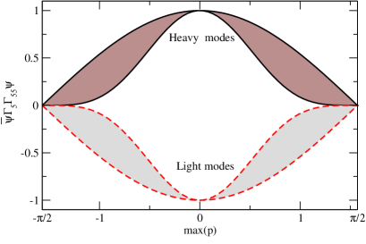
so that at low momenta, the eigenmodes corresponding to $\lambda_{2}$ get a mass of $\pm 2$, while the eigenmodes corresponding to $\lambda_{1}$ are massless.

Finally, the free spectrum of $D_{4}$ reads:

$$\lambda_{1}=-c\frac{\rho}{a}\pm i\sqrt{p^{2}},\quad\lambda_{2}=+c\frac{\rho}{a}\pm i\sqrt{p^{2}},\quad$$ (19)

Note that, in the continuum limit, the point where the spectrum of the $D_{\text{KS}}$ operator intersects the real axis corresponds to four massless modes. By contrast, $D_{2}$ leads to one mode in each of the two intersections away from the origin, and two at the origin. Finally, for $D_{4}$ one obtains two modes at each of the two intersections of the spectrum with the real axis.

The taste chirality of the eigenmodes $\Psi$ of $D_{4}$ and $D_{2}$, is given by $(\bar{\Psi}\Gamma_{55}\Gamma_{5}\Psi)$, where $\Gamma_{55}=\gamma_{5}\otimes\gamma_{5}$ exactly, and $\Gamma_{5}=\gamma_{5}\otimes{\bf 1}+{\cal O}(a)$ in spin $\otimes$ taste. The taste chirality of the eigenmodes corresponding to eigenvalues $\lambda_{1}$ is $c$, while that of the $\lambda_{2}$-eigenvectors is $-c$. This is also depicted in Fig. 2; one can see that the taste chirality of the real eigenmodes is $\pm 1$, and is the same ($+1$ or $-1$) for all modes in a given branch of the $D_{4}$ or $D_{2}$ spectrum. The implications of a well-defined taste chirality have been stressed in [2]: if $\Gamma_{55}\Gamma_{5}\approx\pm 1$, then $\Gamma_{55}\approx\pm\Gamma_{5}$, so that the spin chirality of the real eigenmodes can be probed by $\Gamma_{55}$. This is the reason why the index theorem applies to $D_{2}$ and $D_{4}$, while it does not for $D_{\text{KS}}$ (where both the $\pm 1$ taste chiralities lay on the same single branch.)

Figure 2: (Left) Taste chirality properties of the $D_{2}$ and $D_{4}$ eigenvectors, as a function of (the component of minimum modulus of) their momentum, in the free limit. On an infinite lattice, the eigenvectors associated with real eigenvalues have vanishing momentum and a well-defined taste chirality $\pm 1$. For eigenmodes corresponding to eigenvalue $\lambda_{1}$, the taste chirality becomes $+1$, while for $\lambda_{2}$-eigenmodes the taste chirality approaches $-1$. (Right) The taste chiralities of the eigenmodes of the $D_{2}$ operator; the size of the points corresponds to the magnitude of $c$, while the color indicates the sign: blue for $+c$, red for $-c$.

A shift of the spectra by a real value can thus lead to chiral low-momentum zero modes in each branch, and hence to the possibility of constructing an appropriate index. A common way to study the index consists of looking at the flow of eigenvalues $\lambda(m)$ of:

$$H(m)=\gamma_{5}(D+m).$$ (20)

In general, if $(D+m)$ has a zero-mode $|\Psi_{0}\rangle$ for $m=m_{0}$, then, correspondingly, $H$ has a vanishing eigenvalue $\lambda(m_{0})=0$. With a small perturbation of $m$ away from $m_{0}$, i.e. $m=m_{0}+\delta m$, at leading order the eigenvalues get displaced by an amount $\langle\Psi_{0}|\gamma_{5}(m-m_{0})|\Psi_{0}\rangle$, namely one finds crossings $\lambda(m)=\pm(m-m_{0})$, if $|\Psi_{0}\rangle$ is a chiral mode: $\langle\Psi_{0}|\gamma_{5}|\Psi_{0}\rangle=\pm 1$. As pointed out in [19], the saturation of $(\bar{\Psi}\Gamma_{55}\Gamma_{5}\Psi)$ at value $\pm 1$ discussed above allows us to trade $\Gamma_{5}$ for $\Gamma_{55}$ and use the latter in eq.(20).

An alternative way to look at the spectral flow was proposed in ref. [1] for the $D_{4}$ operator, by studying the eigenvalues of

$$\hat{H}(\rho)=\Gamma_{55}D_{\text{KS}}-\frac{\rho}{a}\Gamma_{5}.$$ (21)

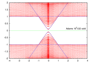
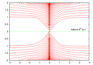
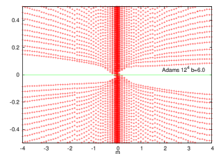
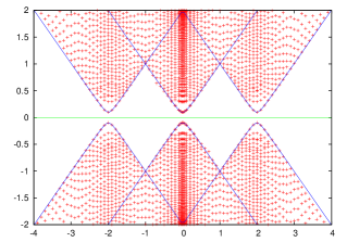
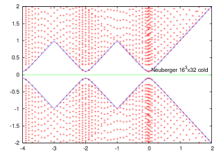
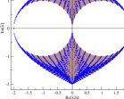
Fig. 3 displays a comparison of the two different ways to define the spectral flow for the $D_{4}$ operator (see [15] for a recent related study): the plots in the top row show the flow of eigenvalues of $\hat{H}$ as a function of $\rho$ (eq.(21)), whereas those in the bottom row refer to the “standard” definition of the flow, using eq. (20). In each row, the left panel displays the results from a cold (i.e., free) configuration on a lattice of size $16^{3}\times 32$, while the central panel is obtained from a cooled configuration of topological charge $Q=1$ on a lattice of size $8^{4}$, and finally the right panel displays the results from a “rough” (i.e., non-cooled) quenched $Q=-1$ configuration at $\beta=6/g^{2}=6$, on a lattice of size $12^{4}$. In the latter case, the comparison of the two flow definitions shows that, with the standard definition, the region around the real axis is populated by a large number of eigenvalues, preventing one from identifying the crossing with accuracy.

Figure 3: Comparison of the spectral flow for the $D_{4}$ operator as obtained from the eigenvalues of the operators defined in eq. (21) (top row panels) and eq. (20) (bottom panels). The three plots (from left to right) in each row show, respectively, the eigenvalues of $\tilde{H}$ (or $H$) as a function of $\rho/a$ (or $m$) from a free configuration on a lattice of size $16^{3}\times 32$, from a cooled configuration of topological charge $Q=1$ on a lattice of size $8^{4}$, and from a non-cooled $Q=-1$ gauge configuration at $\beta=6$, on a lattice of size $12^{4}$.

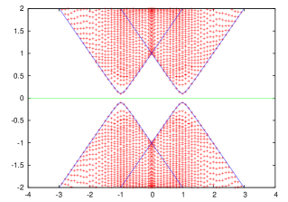
Next, it is interesting to compare the identification of the index, using the spectral flow defined from eq. (20), for staggered fermions with a taste-dependent mass term, and for conventional Wilson fermions. This is shown in Fig. 4: the left, central and right plot in each row show the spectral flow for $D_{4}$, $D_{2}$ and a standard Wilson operator, respectively, while the three different rows, from top to bottom, refer to a cold configuration, to a cooled $Q=1$ configuration, and to a non- cooled $Q=-1$ quenched configuration at $\beta=6$. It is interesting to observe that, as expected, the spectral flow on a cooled instanton configuration clearly reveals $N_{f}\times Q$ crossings. However, one already sees that in the plots of the $\beta=6$ configuration the gap tends to close. This is especially the case for the $D_{4}$ operator, and is related to the properties that will be discussed in Section 3.

Figure 4: Spectral flows for $D_{4}$ (left), $D_{2}$ (center) and a standard Wilson operator (right), on a cold configuration (top), on a cooled $Q=1$ configuration (middle), and on a non-cooled $Q=-1$ quenched configuration at $\beta=6$ (bottom). The solid blue lines in the top row show analytic results.

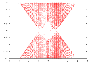
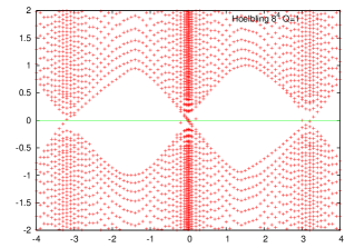
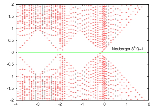
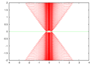
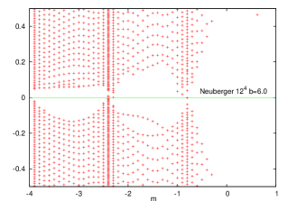
The overall message that can already be drawn from these observations (before addressing a full-fledged numerical investigation) is that the gauge field fluctuations in interacting configurations reduce the width of the gap in the spectrum, and blur the distinction between light modes and doublers.

3 Numerical investigation on interacting configurations

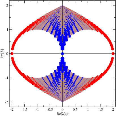
As we showed in the previous section, the fluctuations in typical interacting configurations lead to a filling of the gap in the spectral flow for the various lattice Dirac operators that we are considering, making a proper identification of the index difficult. A related effect can also be seen directly in the spectra of the operators: the panels in Fig. 5 show a comparison of the spectra of $D_{4}$ (top row) and $D_{2}$ (bottom row) in the free case (left), and in interacting configurations at $\beta=6$ (central panels, in which different values of $\rho/a$ or $m$ are used) and at $\beta=5.8$ (right). The figure shows evidence for the superior robustness of lattice fermions based on the $D_{2}$ operator, over $D_{4}$: at $\beta=5.8$ for example, a gap remains clearly visible for $D_{2}$, while it has all but disappeared for $D_{4}$.

This can be understood from the fact that, since $D_{4}$ involves 4-link parallel transporters, it is more sensitive to the gauge field fluctuations in interacting configurations than $D_{2}$ which involves 2-link transporters only.

           

Figure 5: Spectra of $D_{4}$ (top) and $D_{2}$ (bottom) on different types of configurations. As compared to the free case (left), the gap in the spectrum of eigenvalues of $D_{4}$ on interacting configurations tends to close more rapidly than in the case of $D_{2}$. The second and third plot in each row are obtained from quenched configurations at $\beta=6$ (in the third plot on the top row, symbols of different colors correspond to different values of $\rho/a$). Finally, the plots on the right are obtained from a coarser lattice, at $\beta=5.8$ (roundoff errors cause some breaking of the complex conjugation symmetry of the spectrum).

However, for practical applications in large-scale simulations, it is important to remark that, as usual, the effect of gauge fluctuations can be considerably reduced through some suitably optimized smearing procedure.

Next, we considered the effectiveness of these operators for spectroscopy calculations. To this end, we performed a simple test, by studying the mass $m_{PS}$ of the lightest meson in the pseudoscalar channel (the pion). We computed the quark propagator $G(x,y,z,t)$ from a point source, on quenched configurations at $\beta=6$ on a lattice of size $16^{3}\times 32$, then we evaluated the ${\bf p}={\bf 0}$ correlation function

$$C(t)=\sum_{xyz}G(x,y,z,t)\Gamma_{55}G(x,y,z,t)^{\dagger}\Gamma_{55}=\sum_{xyz}|G(x,y,z,t)|^{2},$$ (22)

and extracted $am_{PS}$ searching for the large-time plateau in the effective mass plot, as a function of $t$. Monitoring the behavior of $(am_{PS})^{2}$ as a function of $(am)$, one can study the partially conserved axial current and the issues related to mass renormalization.

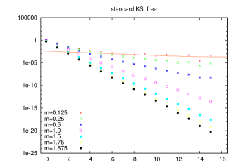
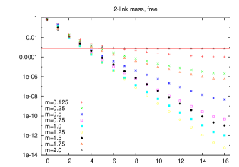
Fig. 6 shows the correlators obtained on a free configuration, for $D_{0}$ (left panel), for $D_{2}$ (central panel) and for $D_{4}$ (right panel). As expected, the $D_{2}$ operator leads to a massless pion for both $am=0$ and $am=2$.

Figure 6: The exponential decay of the correlation function associated with the lightest meson in the pseudoscalar channel for $D_{0}$ (left), for $D_{2}$ (center) and $D_{4}$ (right panel) on a free configuration, for different values of the bare quark mass.

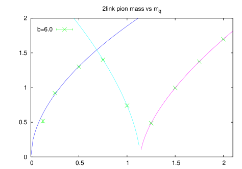
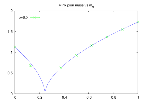
For an interacting configuration (at $\beta=6$), the comparison between $D_{2}$ and $D_{4}$ shown in Fig. 7 reveals that for $D_{2}$ one obtains a massless pion at approximately $am\sim 1.15$, while for $D_{4}$ the same happens for $am\sim 0.25$. Comparing these numbers with the values of the bare masses corresponding to a massless pseudoscalar state in the free limit (1 and 2 respectively), these results give an indication that the mass renormalization is more pronounced for $D_{4}$ than for $D_{2}$. Quantitatively, one can observe that the renormalization factor grows exponentially with the length of the parallel transporters used: $(0.25/1)^{1/4}\sim(1.15/2)^{1/2}$, in agreement with the fact that $D_{4}$ involves 4-link terms, as opposed to $D_{2}$, in which the mass term is constructed from 2- link terms.

Remarkably, with the $D_{2}$ operator, the pion mass shows a square-root behaviour of three different kinds: one can approach the critical bare quark mass $am_{0}\sim 1.15$ from the left or from the right, i.e. from the inside or the outside of the $D_{2}$ spectrum (the behaviour is square-root-like even though the theory describes one flavour only – it is caused by the approach to the Aoki phase). In addition, one can also approach the other critical quark mass $am=0$, corresponding to the central branch of the spectrum, which remains zero as in the free case by symmetry of the average spectrum. The transition from one branch to another seems rather abrupt, and the scaling of the pion mass can be observed over a broad range of quark masses approaching zero.

The lesson is that $D_{2}$ may provide a cost-effective way to simulate $N_{f}=2$ light quark species, without fine-tuning of the bare quark mass to approach the chiral limit.

Figure 7: Tuning of the bare quark mass to obtain a light pion: the two plots show the pion mass as a function of the bare quark mass, for $D_{2}$ (left panel) and $D_{4}$ (right panel) at $\beta=6$.

4 Conclusions

In this work, we performed a numerical study of staggered Dirac operators with a taste-dependent mass term. We restricted our attention to operators including mass terms with tensor or pseudoscalar structure in taste space: their $\gamma_{5}$-hermiticity properties are such, that their eigenvalues come in complex conjugate pairs (as is the case for the usual staggered Dirac operator), leading to a real fermionic determinant, which is non-negative in the absence of negative real eigenvalues.

Such operators were proposed by Adams [1, 2] and by Hoelbling [3]. We compared their properties both in the free limit and on interacting configurations at typical values of the gauge coupling.

Our results show that these operators can indeed be used to separate the low-lying modes and reduce the number of tastes, in a way characterized by well-defined topological properties. Our study of the spectral flow reveals that, for the 4-link operator (with a taste-pseudoscalar mass term), the gap in the eigenvalue spectrum tends to close rather early, obstructing an easy identification of the eigenvalue crossings, which are related to the index. As one might have expected, the 2-link operator shows markedly more robustness to gauge fluctuations.

We also performed an elementary study of pion propagators, which shows that the lightest meson is rather easy to isolate without explicitly disentangling spin and taste degrees of freedom. Approaching the chiral limit requires in general the fine-tuning of an additive mass term, as for Wilson fermions. One important exception occurs for the 2-link operator: if one chooses the middle branch of the spectrum, one can study a theory with two tastes, where the additive mass renormalization vanishes due to the symmetry of the spectrum. Therefore, no fine-tuning is needed.

Although the 2-link operator was designed to produce a single taste (with a fine-tuned additive mass), it may well be that its most promising use is to simulate two tastes without additive mass renormalization. Note that the heavy doubler modes do not completely decouple in that situation. In the background of a topological charge $Q$, they contribute real eigenvalues $\sim(+1/a)^{Q}$ and $(-1/a)^{Q}$, making the determinant negative when $Q$ is odd. The $\theta$-parameter is thus equal to $\pi$. This sign $(-1)^{Q}$ should be removed by hand (or simply ignored) in order to simulate the $\theta=0$ theory.

Finally, we studied the properties of an overlap operator with a $D_{4}$ kernel (see Appendix). We found that its locality properties are similar to those of the operator based on a Wilson kernel. As it concerns the computational cost for a quark propagator calculation, we found that, in the free limit or on very smooth gauge configurations, the inversion of the operator based on a kernel with a four-link mass term is almost one order of magnitude faster than using an overlap with Wilson kernel. However, we also observed a significant loss of efficiency on interacting (quenched) configurations at $\beta=6$, where the operator with the $D_{4}$ kernel is only approximately twice as fast as that with a Wilson kernel. The reason for this can probably be traced back to the fact that the four-link transporters in the mass term are more sensitive to the effect of the fluctuations in gauge configurations on coarser lattices. Our crude assessment indicates that this new, staggered, overlap operator does not bring a major computational advantage over a Wilson kernel, while producing two degenerate flavors, but without the full $SU(2)$ flavor symmetry.

Two copies of an overlap operator with a kernel based on Hoelbling’s 2-link operator would give more flexibility, e.g. that of simulating two flavors with unequal masses, for a similar computer effort.

Note added: After this paper was completed, a difficulty with the Hoelbling operator $D_{2}$ eq.(3) was pointed out by Steve Sharpe, and clarified by David Adams, during the Yukawa Institute Workshop “New Types of Fermions on the Lattice”. It appears that the Hoelbling operator lacks sufficient rotational symmetry, so that fine-tuned Wilson loop counterterms will presumably be needed to maintain hypercubic rotational symmetry in unquenched simulations. Adams’ operator $D_{4}$ eq.(8) does not suffer from this problem.

Appendix A Staggered overlap operator

We also studied the properties of an overlap operator based on a staggered $D_{4}$ kernel, as originally proposed in [1]. The construction is completely standard:

$$D_{\mbox{\tiny{ov}}}=\frac{\rho}{a}\left(1+\frac{D_{4}}{\sqrt{D_{4}^{\dagger}D_{4}}}\right)$$ (A.1)

and leads to two exactly massless physical fermions in the continuum limit, without fine-tuning. As compared to a conventional overlap operator based on a Wilson kernel, the potential advantages of this construction are related to the reduced kernel size ($D_{4}$ is a matrix of size four times smaller than a Wilson operator on the same lattice). We take $\rho=1$.

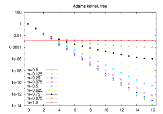
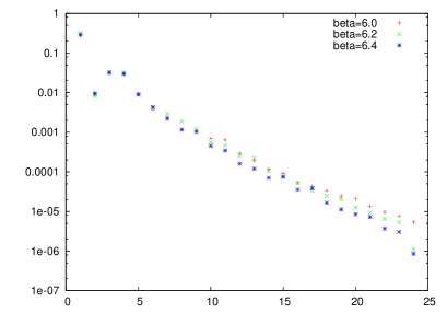
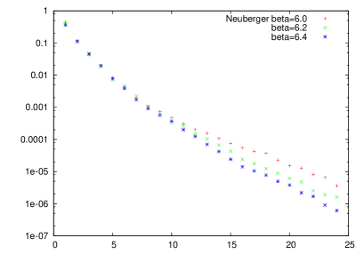
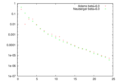
To understand the effectiveness of an overlap operator with a $D_{4}$ kernel, the first important issue to be discussed is the locality of the operator. As is well-known, an overlap operator is not ultra-local [21]. Its locality properties can be studied by looking at the decay of its matrix elements between source and sink at sites $x$ and $y$ (which we denote as $M_{x,y}$, where, for simplicity, we only show the indices corresponding to the site coordinates), as a function of the distance between $x$ and $y$ [22]. To this end, in the two plots at the top of Fig. 8 we show the decay of $|M_{x,y}|$ against $|x-y|_{1}$, the 1-norm distance (or “Manhattan distance”) between the sites $x$ and $y$, comparing the matrix elements of an overlap operator obtained using a $D_{4}$ kernel (left panel) or a conventional Wilson kernel (right panel). Although the $D_{4}$ kernel is less local than the Wilson kernel, the locality properties of the corresponding overlap operators are comparable. This appears quite clearly in the plots displayed at the bottom of the figure, in which the results for the two operators are shown together, for a cold configuration (left panel) and for a configuration at $\beta=6$ (right panel).

Figure 8: The plots at the top of the figure show the decay of the matrix elements of an overlap operator obtained using a $D_{4}$ kernel (left) or a Wilson kernel (right), as a function of the 1- norm distance between the sites. The results from the two operators are displayed together in the two bottom plots, for a cold (bottom left panel) and a $\beta=6$ configuration (bottom right panel).

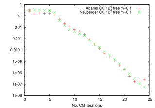
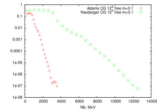
Another important factor in the efficiency of a lattice Dirac operator is the cost of applying the operator to a vector. The multiplication by the kernel is about twice as fast, if one uses $D_{4}$ instead of a Wilson kernel (staggered fields do not have an explicit spinor index but $D_{4}$ has twice as many non-zero elements as the Wilson operator). In the computation of the sign of $\tilde{H}=\Gamma_{55}D_{4}$, using the conjugate gradient (CG) method, and no deflation, the gain with respect to a conventional Wilson kernel is a factor ranging from approximately 2-3 to about 8. However, these numbers are only gross estimates, and could be improved, e.g., by optimizing the parameters of the $D_{4}$ kernel. Similarly, an improved form for the kinetic operator, link smearing (for the kinetic and/or the mass term), and standard tricks related to deflation, preconditioning, etc… could be applied.

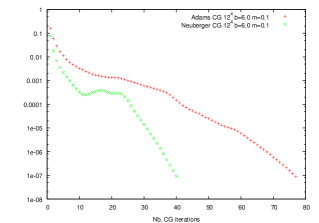
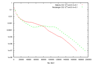
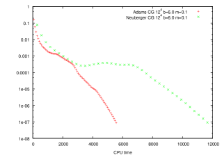
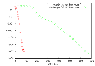
To discuss the computational cost of the inversion of the operator, we compared the two overlap operators on the same pure-glue, $\beta=6$, background on a $12^{4}$ lattice, using the same, basic, inner/outer CG algorithm. In our computation, we evaluated the propagator as the solution of the equation:

$$(D_{ov}+m)^{\dagger}(D_{ov}+m)x=(D_{ov}+m)^{\dagger}b$$ (A.2)

with $ma=0.1$, using a conjugate gradient (CG) iterative solver: at each iteration, ${\rm sign}(H)$ is applied to a vector $v$ through a 2-pass Lanczos process. One builds a tridiagonal matrix $T$ and takes the signs of its eigenvalues (which are representative of those of $H$), then reconstructs ${\rm sign}(H)v$, as described in ref. [24]. The results are displayed at the top of Fig. 8: the three plots (from left to right) show the computational cost for the outer CG iteration, for the matrix-times-vector multiplication, and the total CPU cost. For comparison, we also show the analogous results in the free-field case, in the plots at the bottom of the figure. This comparison shows that the computational advantages expected from elementary arguments, and observed in the free limit, turn out to be dramatically reduced in “realistic” interacting configurations. Again, this reduction points to a reduction in the eigenvalue gap of $D_{4}$.

Figure 9: Top row: Comparison of the computational costs for the overlap operator inversion at a given level of precision, using a $D_{4}$ (red points) or a Wilson (green symbols) kernel: the left panel displays the costs related to the outer CG iteration, the central plot shows the costs of the matrix-times-vector multiplication, and finally the right panel displays the total CPU cost. For comparison, the plots in the bottom row show the analogous results for a free configuration.

References

- [1] D. H. Adams, Phys. Rev. Lett. 104 (2010) 141602. [arXiv:0912.2850 [hep-lat]].
- [2] D. H. Adams, Phys. Lett. B 699 (2011) 394 [arXiv:1008.2833 [hep-lat]].
- [3] C. Hoelbling, Phys. Lett. B696 (2011) 422. [arXiv:1009.5362 [hep-lat]].
- [4] H. B. Nielsen, M. Ninomiya, Phys. Lett. B105 (1981) 219; Nucl. Phys. B185 (1981) 20; [Erratum-ibid. B195 (1982) 541]. Nucl. Phys. B193 (1981) 173. D. Friedan, Commun. Math. Phys. 85 (1982) 481.
- [5] M. Lüscher, Phys. Lett. B428 (1998) 342 [hep-lat/9802011].
- [6] P. H. Ginsparg, K. G. Wilson, Phys. Rev. D25 (1982) 2649.
- [7] D. B. Kaplan, Phys. Lett. B288 (1992) 342 [hep-lat/9206013]. H. Neuberger, Phys. Lett. B417 (1998) 141 [hep-lat/9707022]. P. Hasenfratz, V. Laliena, F. Niedermayer, Phys. Lett. B427 (1998) 125 [hep-lat/9801021].
- [8] K. G. Wilson, in New Phenomena in Subnuclear Physics, ed. A. Zichichi (Plenum Press, 1977).
- [9] J. B. Kogut, L. Susskind, Phys. Rev. D11 (1975) 395.
- [10] E. Follana et al. [HPQCD and UKQCD Collaborations], Phys. Rev. D 72 (2005) 054501 [hep-lat/0507011].
- [11] S. Durr and C. Hoelbling, Phys. Rev. D 69 (2004) 034503 [hep-lat/0311002]; S. Durr, C. Hoelbling and U. Wenger, Phys. Rev. D 70 (2004) 094502 [hep-lat/0406027]; F. Bruckmann et al., Phys. Rev. D 78 (2008) 034503 [arXiv:0804.3929 [hep-lat]]; PoS LAT 2007 (2007) 274 [arXiv:0802.0662 [hep-lat]].
- [12] M. Creutz, PoS CONFINEMENT 8 (2008) 016 [arXiv:0810.4526 [hep-lat]]. G. C. Donald, C. T. H. Davies, E. Follana and A. S. Kronfeld, Phys. Rev. D 84 (2011) 054504 [arXiv:1106.2412 [hep-lat]].
-
[13]
P. de Forcrand, A. Kurkela, M. Panero,
PoS LATTICE2010 (2010) 080
[arXiv:1102.1000 [hep-lat]];
see also
http://super.bu.edu/~brower/qcdna6/talks/deforcrand.pdf. - [14] L. H. Karsten, Phys. Lett. B 104 (1981) 315. F. Wilczek, Phys. Rev. Lett. 59 (1987) 2397. M. Creutz, JHEP 0804 (2008) 017 [arXiv:0712.1201 [hep-lat]]. A. Boriçi, Phys. Rev. D 78 (2008) 074504 [arXiv:0712.4401 [hep-lat]]. S. Capitani et al., JHEP 1009 (2010) 027 [arXiv:1006.2009 [hep-lat]]. M. Creutz, T. Kimura and T. Misumi, JHEP 1012 (2010) 041 [arXiv:1011.0761 [hep-lat]]; PoS LATTICE 2011 (2011) 106 [arXiv:1110.2482 [hep-lat]]; T. Kimura, S. Komatsu, T. Misumi, T. Noumi, S. Torii and S. Aoki, JHEP 1201 (2012) 048 [arXiv:1111.0402 [hep-lat]].
- [15] E. Follana, V. Azcoiti, G. Di Carlo and A. Vaquero, PoS LATTICE 2011 (2011) 100 [arXiv:1111.3502 [hep-lat]].
- [16] H. S. Sharatchandra, H. J. Thun, P. Weisz, Nucl. Phys. B192 (1981) 205. F. Gliozzi, Nucl. Phys. B204 (1982) 419. C. van den Doel, J. Smit, Nucl. Phys. B228 (1983) 122. H. Kluberg-Stern et al., Nucl. Phys. B220 (1983) 447.
- [17] M. F. L. Golterman, J. Smit, Nucl. Phys. B245 (1984) 61.
- [18] P. de Forcrand, PoS LAT 2009 (2009) 010 [arXiv:1005.0539 [hep-lat]].
- [19] D. H. Adams, PoS LATTICE 2010 (2010) 073 [arXiv:1103.6191 [hep-lat]].
- [20] P. de Forcrand, M. García Pérez, J. E. Hetrick, E. Laermann, J. F. Lagae, I. O. Stamatescu, Nucl. Phys. Proc. Suppl. 73 (1999) 578. [hep-lat/9810033].
- [21] I. Horváth, Phys. Rev. Lett. 81 (1998) 4063. [hep-lat/9808002].
- [22] P. Hernández, K. Jansen, M. Lüscher, Nucl. Phys. B552 (1999) 363. [hep-lat/9808010].
- [23] W. Bietenholz, Fortsch. Phys. 56 (2008) 107. [hep-lat/0611030]. S. Dürr, G. Koutsou, [arXiv:1012.3615 [hep-lat]].
- [24] A. Boriçi, Phys. Lett. B453 (1999) 46. [hep-lat/9810064].