Critical configurations of planar robot arms

Abstract.

It is known that a closed polygon $P$ is a critical point of the oriented area function if and only if $P$ is a cyclic polygon, that is, $P$ can be inscribed in a circle. Moreover, there is a short formula for the Morse index. Going further in this direction, we extend these results to the case of open polygonal chains, or robot arms. We introduce the notion of the oriented area for an open polygonal chain, prove that critical points are exactly the cyclic configurations with antipodal endpoints and derive a formula for the Morse index of a critical configuration.

1. Introduction

Geometry of various special configurations of robot arms modeled by open polygonal chains appears essential in many problems of mechanics, robot engineering and control theory. The present paper is concerned with certain planar configurations of robot arms appearing as critical points of the oriented area considered as a function on the moduli space of the arm in question. This setting naturally arose in the framework of a general approach to extremal problems on configuration spaces of mechanical linkages developed in [5], [6], [8], which has led to a number of new results on the geometry of cyclic polygons [9], [7] and suggested a variety of open problems. The approach and results of [5], [6] provided a paradigm and basis for the developments presented in this paper.

Let us now outline the structure and main results of the paper. We begin with recalling necessary definitions and basic results concerned with moduli spaces and cyclic configurations. In the second section we prove that critical configurations of a planar robot arm are given by the cyclic configurations with diametrical endpoints called diacyclic (Theorem 1) and describe the structure of all cyclic configurations of a robot arm (Theorem 2). Next, we establish that, for a generic collection of lengths of the links, the oriented area is a Morse function on the moduli space (Theorem 3) and provide some explications in the case of a 3-arm. In the last section we prove an explicit formula for the Morse index of a diacyclic configuration (Theorem 6) and illustrate it by a few visual examples. In conclusion we briefly discuss several open problems and related topics.

Acknowledgements. We are grateful to ICTP, MFO, and CIRM. It’s our special pleasure to acknowledge the excellent working conditions in these institutes.

2. Oriented area function for planar robot arm

Let $L=(l_{1},\ldots,l_{n}),\ L\in\mathbb{R}^{n}_{+}$. Informally, a robot arm, or an open polygonal chain is defined as a linkage built up from rigid bars (edges) of lengths $l_{i}$ consecutively joined at the vertices by revolving joints. It lies in the plane, its vertices may move, and the edges may freely rotate around endpoints and intersect each other. This makes various planar configurations of the robot arm.

Let us make this precise. A configuration of a robot arm is defined as a $n+1$-tuple of points $R=(r_{0},\ldots,r_{n})$ in the Euclidean plane $\mathbb{R}^{2}$ such that $|r_{i-1}r_{i}|=l_{i},i=1,\ldots,n$. Each configuration carries a natural orientation given by vertices’ order.

To factor out the action of orientation-preserving isometries of the plane $\mathbb{R}^{2}$, we consider only configurations with two first vertices fixed: $r_{0}=(0,0)$, $r_{1}=(l_{1},0)$. The set of all such planar configurations of a robot arm is called the moduli space of a robot arm. We denote it by $M^{0}(L)$. It is a subset of Euclidean space $\mathbb{R}^{2n-2}$ and inherits its topology and a differentiable space structure so that one can speak of smooth mappings and diffeomorphisms in this context. After these preparations it is obvious that the moduli space of any planar robot arm is diffeomorphic to the torus $(S^{1})^{n-1}$. We will use its parametrization by angle-coordinates $\beta_{i}$ (that is, by angles between $r_{0}r_{1}$ and $r_{k}r_{k+1},k=1,\ldots,n-1$).

In this paper we consider the oriented (signed) area as a function on $M^{0}(L)$.

Definition 1.

For any configuration $R$ of $L$ with vertices $r_{i}=(x_{i},y_{i}),\ i=0,\ldots,n$, its (doubled) oriented area A(R) is defined by

$$2A(R)=(x_{0}y_{1}-x_{1}y_{0})+\cdots+(x_{n}y_{0}-x_{0}y_{n}).$$

In other words, we add the connecting side $r_{n}r_{0}$ turning a given configuration $R$ into a $(n+1)$-gon and compute the oriented area of the latter. Obviously, $A(R)$ is a smooth function on the moduli space $M^{0}(L)$ of any robot arm $L$.

3. Critical configurations. 3-arms.

A configuration $R=(r_{0},\ldots,r_{n})$ of a robot arm $L=(l_{1},\ldots,l_{n})$ is cyclic if all its vertices lie on a circle.

A configuration is quasicyclic (a QC-configuration for short) if all its vertices lie either on a circle or on a (straight) line.

A configuration is closed cyclic if the last and the first vertices coincide: $r_{0}=r_{n}$.

A configuration is diacyclic if it is cyclic and the ”connecting side” $r_{n},r_{0}$ is a diameter of the circumscribed circle (”diacyclic” is a sort of shorthand for ”diametrally cyclic”). In other words, the connecting side $r_{n}r_{0}$ passes through the center of the circumscribed circle or, equivalently, each interval $r_{0}r_{k}$ is orthogonal to the interval $r_{k}r_{n}$ for $k=1,\ldots,n-1$.

Theorem 1.

For any robot arm $L\in\mathbb{R}^{n}_{+}$, critical points of $A$ on the moduli space $M^{0}(L)$ are exactly the diacyclic configurations of $L$.

Proof.

As above, we assume that $r_{0}=(0,0)$,  $r_{1}=(l_{1},0)$. For a configuration $R=(r_{0},\ldots,r_{n})$ we put $e_{i}={r_{i}-r_{i+1}},i=1,\ldots,n$. Obviously, ${r_{i}}={e_{1}}+\cdots+{e_{i}}$ and ${e_{i}}=l_{i}(cos\beta_{i},sin\beta_{i})$. Denote by ${a}\times{b}$ the oriented area of the parallelogram spanned by vectors $a$ and ${b}$ (i.e., we take the third coordinate of their vector product). The differentiation of vectors ${e_{i}}$ with respect to angular coordinates $\beta_{j}$ will be denoted by upper dots (i.e., there will appear terms of the form $\dot{e_{i}}$). With these assumptions and notations we can write

$$A=\sum^{n}_{j=1}r_{j-1}\times r_{j}=\sum^{n}_{j=2}(e_{1}+\cdots+e_{j-1})\times e_{j}=\sum_{1\leq i<j\leq n}e_{i}\times e_{j}.$$

Taking partial derivatives with respect to $\beta_{k},\ k=2,\ldots,n$ we get

$$\frac{\partial A}{\partial\beta_{k}}=-\sum^{k-1}_{i=1}{e_{i}}\times\dot{e_{k}}+\sum^{k-1}_{i=1}e_{k}\times\dot{e_{i}}.$$

Notice now the identities:

$$\dot{e_{i}}\times e_{j}=e_{i}\cdot e_{j}=-e_{i}\times\dot{e_{j}}.$$

Eventually we get:

$$\frac{\partial A}{\partial\beta_{k}}=-\sum^{k-1}_{i=1}e_{k}\cdot e_{i}+\sum^{n}_{i=k+1}e_{k}\cdot e_{i}=(-\sum^{k-1}_{i=1}e_{i}+\sum^{n}_{i=k+1}e_{i})\cdot e_{k}.$$

Consider now the equations $\frac{\partial A}{\partial\beta_{k}}=0,\ k=2,\ldots,n$ defining the critical set of A. By taking appropriate linear combinations of equations, this system of $n-1$ equations is easily seen to be equivalent to the system of equations:

$$(\sum^{k-1}_{i=1}e_{i})\cdot(\sum^{n}_{i=k}e_{j})=0,\ k=2,\ldots,n.$$

In geometric terms this means that the intervals $r_{0}r_{k-1}$ and $r_{k-1}r_{n}$ are orthogonal for $k=2,\ldots,n$. It remains to refer to Thales theorem to conclude that the points $r_{0},\ldots,r_{n}$ lie on a circle with diameter $r_{0}r_{n}$. ∎

Lemma 1.

The order of the lengths $l_{1},\dots,l_{n}$ does not matter: for any transposition $\sigma$, there exists a diffeomorphism taking $M^{0}(L)$ to $M^{0}(\sigma L)$ which preserves the function $A$, and therefore, all the critical points together with their Morse indices.

The proof (which repeats the proof of the similar lemma for closed polygons from [9]) is as follows. Two consecutive edges of a configuration can be (geometrically) permuted in such a way that the oriented area remains unchanged. Such a geometrical permutation yields a diffeomorphism from one configuration space to another.∎

Theorem 2.

Assume that $l_{1}>l_{i}$ for all $i=2,\dots,n$. Then we have the following:

1. The set of all quasicyclic configurations is a disjoint collection of $2^{(n-2)}$ embedded (topological) circles (QC-components for short).

2. Each of the circles contains at least two critical points of $A$.

3. Assuming that all critical points are Morse non-degenerate, $A$ is a perfect Morse function if and only if each circle has exactly two critical points of $A$.

4. Each of the circles contain exactly two aligned configurations.

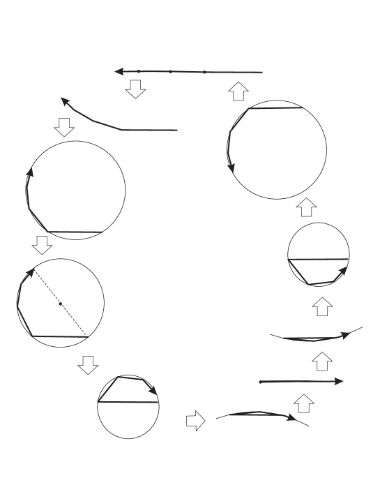
Proof. We shall use the following notation: For a quasicyclic configuration, we define $\varepsilon_{i}=1$ if the center of the circle lies to the left with respect to $r_{i-1}r_{i}$. Otherwise we put $\varepsilon_{i}=-1$.

We show that each collection of signs $\varepsilon_{i}=\pm 1,\ i=3,\dots,n$ yields a (topological) circle of quasicyclic configurations.

Indeed, fix $\varepsilon_{3},\dots,\varepsilon_{n}$. Take a (metric) circle $S(\rho)$ whose radius $\rho$ varies from $l_{1}$ to infinity.

A differentiable coordinate for a QC-component is e.g. the angle between the first and the second arm (mod $2\pi$). The change of this angle induces a differentiable change of the radius $\rho$ and each vertex moves around the intersection of a circle with center $r_{i}$ and radius $l_{i}$, which intersects the circumscribed circle (with radius $\rho$) transversal (due to the condition $l_{1}>l_{i}$).

If $l_{1}<\rho<\infty$, the circle $S(\rho)$ has exactly one (up to a rigid motion) inscribed configuration with $E=(\pm 1,1,\varepsilon_{3},\varepsilon_{4},\dots,\varepsilon_{n})$ and exactly one inscribed configuration with $E(R)=(\pm 1,-1,-\varepsilon_{3},-\varepsilon_{4},\dots,-\varepsilon_{n})$. The QC-component becomes in this way divided into four arcs, each with prescribed type of $E$, parameterized by the radius $\rho$. At the endpoints (that is, if $\rho=l_{1}$ or $\rho=\infty$) the four arcs join. More precisely, the arc that corresponds to $1,1,\varepsilon_{3},\dots,\varepsilon_{n}$ is followed by the arc that corresponds to $-1,1,\varepsilon_{3},\dots,\varepsilon_{n}$, then the next one with $+1,-1,-\varepsilon_{3},\dots,-\varepsilon_{n}$, then to the one with $-1,-1,-\varepsilon_{3},\dots,-\varepsilon_{n}$, and then to $1,1,\varepsilon_{3},\dots,\varepsilon_{n}$ (see Fig. 1). Continuity reasons imply that each such a circle of quasicyclic configurations has at least two diacyclic ones.

Remark 1.

The condition $l_{1}>l_{i}$ is important indeed: if there are several longest edges, the QC-components acquire common points. For instance, for an equilateral arm, they form a connected set.

Remark 2.

A QC-component can contain besides the diacyclic and aligned arms also closed cyclic arms (polygons). All of them occur in this way. These special configurations are related to critical points of functions on configuration spaces (respectively, oriented area of an arm, squared length of the closing interval (see [4], and oriented area of a polygon (see [6]). Note that existence of a closed polygon on a QC-component (as well as the number of diacyclic configurations) depends on $l_{1},\dots,l_{n}$.

Figure 1. A circle of quasicyclic configurations

∎

Theorem 3.

For a generic sidelength vector $L\in\mathbb{R}^{n}_{+}$, the function $A$ has only non-degenerate critical points on $M^{0}(L)$.

Proof.

The proof from [9] is applicable with some evident modifications. Namely, after introducing a local coordinate system with diagonals as coordinates, the Hessian matrix becomes tridiagonal with analytic entries. Deformation arguments show that a perturbation of just two of the edgelengths $l_{i}$ makes the Hessian non-zero. ∎

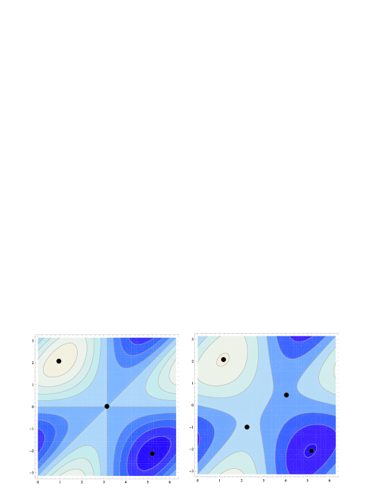
For a $2$-arm we obviously have two points: one maximum and one minimum.

Proposition 1.

Generically, for a 3-arm $A$ has exactly $4$ critical points on $M^{0}(P)$. If $A$ is a Morse function (that is, if the Hessian is non-degenerate), these are two extrema and two saddles (see Fig. 7). Extrema are given by the convex diacyclic configurations.

Figure 2. Diacyclic configurations for a generic $3$-arm

Proof. Partial derivatives give the conditions for critical point:

$$\partial A/\partial\beta_{1}=l_{1}l_{2}cos[\beta_{1}]-l_{2}l_{3}cos[\beta_{2}-\beta_{1}]=0,\,\partial A/\partial\beta_{2}=l_{1}l_{3}cos[\beta_{2}]+l_{2}l_{3}cos[\beta_{2}-\beta_{1}]=0.$$

The orthogonality conditions are simply ${r_{0}r_{1}}\bot({r_{1}r_{2}}+{r_{2}r_{3}}),\,({r_{0}r_{1}}+{r_{1}r_{2}})\bot{r_{2}r_{3}}.$

The next step is to show that there are exactly $4$ critical points. This can be done as follows. One uses elementary geometry to obtain a cubic equation for the length $d$ of the connecting edge:

$$d^{3}=(l_{1}^{2}+l_{2}^{2}+l_{3}^{2})d\pm 2l_{1}l_{2}l_{3}.$$

One has to solve these equations in $d$, taking into account $d\geq l_{1}$ and $d\geq l_{3}$. Elementary calculation shows that both the + equation and the - equation have one solution satisfying these conditions. From $\cos\beta_{1}=\pm l_{3}/d,\,\cos(\beta_{2}-\beta_{1})=\pm l_{1}/d$ it follows that there are exactly two solutions in each case. They occur in pairs $(\beta_{1},\beta_{2}),\,(-\beta_{1},-\beta_{2})$, which gives the result.

Notice that this reasoning shows in all cases, (except for $l_{1}=l_{2}=l_{3}$) that there are four critical points; in the generic case they are all Morse. If $l_{1}=l_{2}=l_{3}$ there are three critical points, one of which is a ”monkey saddle” . Note that in this case we obtain the minimal number of critical points of a differentiable function on a torus. It is equal to the Lusternick-Schnirelmann category of the torus, see [11].

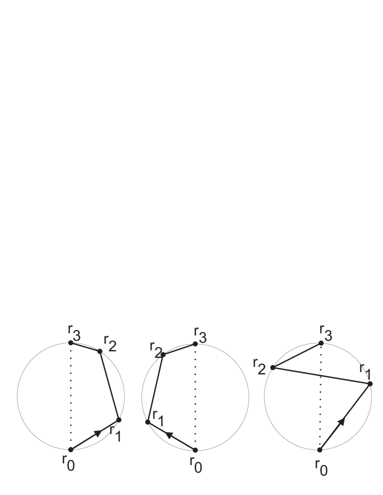
Example 1.

In the case $l_{1}=l_{2}=l_{3}$, there are three critical points on the torus: one maximum of $A$, one minimum, and a monkey saddle point. Figure 3, left depicts the level sets of $A$ on the torus, whereas generically we have Figure 3, right.

Figure 3. Level sets of the function $A$ for $l_{1}=l_{2}=l_{3}$

4. On Morse index of a diacyclic configuration

We start with some examples.

For arbitrary $n>3$, oriented area $A$ may or may not be a perfect Morse function:

Example 2.

Let $n=4$ and $L=(10,3,2,1)$. To be more precise, we take the lengths generically perturbed in order to guarantee non-degenerate critical points. Then configuration space is $M^{0}(L)=(S^{1})^{3}$. Its Betti numbers are $\beta_{0}=1$, $\beta_{1}=3$, $\beta_{2}=3$, $\beta_{3}=1$. Direct computations show, that there are exactly 8 critical points on $M^{0}(L)$ (the four configurations depicted in Fig. 7 and their symmetric images). Therefore for this particular linkage $A$ is a perfect Morse function.

Example 3.

Let now $L=(22,17,21.9,19)$.

Again, $M^{0}(L)=(S^{1})^{3}$. However, direct computations show, that there are more than 8 critical points on $M^{0}(L)$ (the six configurations depicted in Fig. 5 and their symmetric images). Therefore in this case $A$ is not a perfect Morse function. There are two QC-components with 3 diacyclic configurations, whereas all others have only one.

Figure 4. A is a perfect Morse function for $L=(10,3,2,1)$

Figure 5. A is not a perfect Morse function for $L=(22,17,21.9,19)$

Now we are going to find the Morse index of a diacyclic configuration of a robot arm by reducing the problem to the Morse index of a critical configurations of some closed linkage. First, we remind the reader the details about closed linkages. A closed linkage can be described as a flexible polygon on a plane. It is defined by its string of edges $L=(l_{1},\ldots,l_{n}),L\in\mathbb{R}^{n}_{+}$. A configuration of a closed linkage is defined as a n-tuple of points $P=(p_{1},\ldots,p_{n})$ in the Euclidean plane $\mathbb{R}^{2}$ such that $|p_{i}p_{i+1}|=l_{i},i=1,\ldots,n$. Here the numeration is cyclic, i.e. $p_{n+1}=p_{1}$.

Definition 2.

For any configuration $P$ of $L$ with vertices $p_{i}=(x_{i},y_{i}),i=1,\ldots,n$, its (doubled) oriented area $A(R)$ is defined as

$$2A(P)=(x_{1}y_{2}-x_{2}y_{1})+\cdots+(x_{n}y_{1}-x_{1}y_{n}).$$

Generically, the oriented area function is a Morse function on moduli space of a closed linkage.

Theorem 4.

([6]) Generically, a polygon $P$ is a critical point of the oriented area function $A$ iff $P$ is a cyclic configuration. ∎

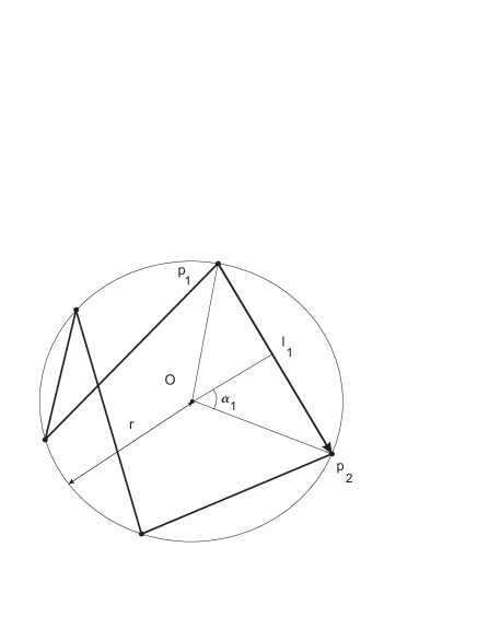
We will use the following notations for cyclic configurations, both open and closed:

$O$ is the center of the circumscribed circle.

$\alpha_{i}$ is the half of the angle between the vectors $\overrightarrow{Op}_{i}$ and $\overrightarrow{Op}_{i+1}$. The angle is defined to be positive, orientation is not involved.

Each edge has an orientation $\varepsilon_{i}$ with respect to the circumscribed circle:

$$\varepsilon_{i}=\left\{\begin{array}[]{ll}1,&\hbox{if the center $O$ lies to the left of }p_{i}p_{i+1};\\ -1,&\hbox{if the center $O$ lies to the right of }p_{i}p_{i+1}.\end{array}\right.$$

$E(P)=(\varepsilon_{1},\dots,\varepsilon_{n})$ is the string of orientations of all the edges.

$e(P)$ is the number of positive entries in $E(P)$.

$\mu_{P}=\mu_{P}(A)$ is the Morse index of the function $A$ at the point $P$.

Figure 6. Notation for a pentagonal cyclic configuration with $E=(-1,-1,-1,1,-1)$

For cyclic configuration $P$ of a closed linkage $\omega_{P}$ is the winding number of $P$ with respect to the center $O$.

Theorem 5.

([7]) For a generic cyclic configuration $P$ of a closed linkage $L$,

$$\mu_{P}(A)=\left\{\begin{array}[]{ll}e(P)-1-2\omega_{P}&\hbox{if }\ \delta(P)>0;\\ e(P)-2-2\omega_{P}&\hbox{otherwise}.\end{array}\right.$$

$$\hbox{Here}\ \ \delta P=\sum_{i=1}^{n}\varepsilon_{i}\tan\alpha_{i}.\qed$$

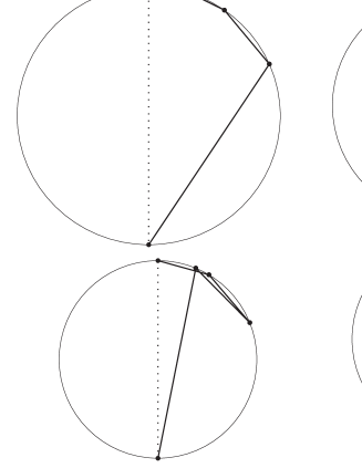
Returning to open chains, let $R$ be a diacyclic configuration. Define its closure $R^{Cl}$ as a closed cyclic polygon obtained from $R$ by adding two positively oriented edges (see Fig. 7) and denote by $\omega_{R}$ the winding number of the polygon $R^{Cl}$ with respect to the center $O$. After this preparation we can present the below formula for the Morse index.

Theorem 6.

Let $L=(l_{1},\ldots,l_{n})$ be a generic open linkage, and let $R$ be one of its critical configuration. For the Morse index $\mu_{R}(A)$ of the oriented area function $A$ at the point $R$, we have

$$\mu_{R}(A)=\left\{\begin{array}[]{ll}e(R)-2\omega_{R}+1&\hbox{if ~{}}\delta(R)>0,\\ e(R)-2\omega_{R}&\hbox{otherwise.}\end{array}\right.$$

$$\hbox{Here}\ \ \delta R=\sum_{i=1}^{n}\varepsilon_{i}\tan\alpha_{i}.$$

Proof.

Figure 7. An open chain, its symmetry image, duplication and closure

Figure 8. The mapping $\phi$ splits a closed chain into two open chains

Consider the manifold $M^{\circ}_{2}(L)\times M^{\circ}_{2}(L)=\{R_{1}\times R_{2}:\ R_{1},R_{2}\in M^{\circ}_{2}(L)\}$. Generically, the function $A(R_{1}\times R_{2})=A(R_{1})+A(R_{2})$ is a Morse function on $M^{\circ}_{2}(L)\times M^{\circ}_{2}(L)$.

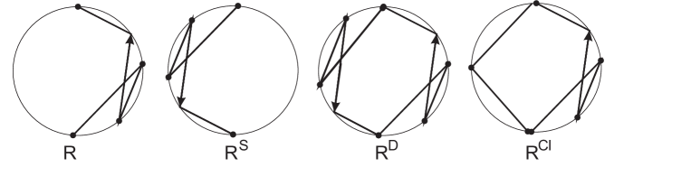
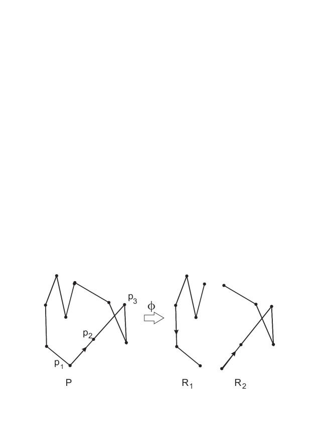
Next, define the duplication of $L$ as the closed linkage $L^{D}=(l_{1},l_{2},\ldots,l_{n},l_{1},l_{2},\ldots,l_{n})$.

Consider a mapping $\phi$ which splits a polygon $P\in L^{D}$ into two open chains, $R_{1}$ and $R_{2}$. The mapping $\phi$ embeds $M_{2}(L^{D})$ as a codimension one submanifold of $M^{\circ}_{2}(L)\times M^{\circ}_{2}(L)$.

For a cyclic open chain $R$, define $R^{S}$ as the symmetric image of $R$ with respect to the center $O$. Define also $R^{D}\in M_{2}(L^{D})$ as a cyclic closed polygon obtained by patching together $R$ and $R^{S}$. By Theorem 4, $R^{D}$ is a critical point of the oriented area.

On the one hand, the Morse index of its image $\phi(R^{D})=R\times R^{S}$ on the manifold $M^{\circ}_{2}(L)\times M^{\circ}_{2}(L)$ equals $2\mu_{R}$. On the other hand, the Morse index of $R^{D}$ on the manifold $M_{2}(L^{D})$ is known by Theorem 5.

Since $M_{2}(L^{D})$ embeds as a codimension one submanifold of $M^{\circ}_{2}(L)\times M^{\circ}_{2}(L)$, the Morse indices differ at most by one. More precisely, we have the following lemma:

Lemma 2.

Either $\mu_{R^{D}}=2\mu_{R}$, or $\mu_{R^{D}}=2\mu_{R}-1.\qed$

By Theorem 5,

$$\mu_{R^{D}}=\left\{\begin{array}[]{ll}e(R^{D})-2\omega(R^{D})-1&\hbox{ if }\delta(R^{D})>0,\\ e(R^{D})-2\omega(R^{D})-2&\hbox{ otherwise.}\end{array}\right.$$

Clearly, we have $e(R^{D})=2e(R)$,   $\delta(R^{D})=2\delta(R)$, and $\omega(R^{D})=2\omega(R)-1$. This gives us

$$\mu_{R^{D}}=\left\{\begin{array}[]{ll}2e(R)-4\omega(R)+1&\hbox{if }\delta(R)>0,\\ 2e(R)-4\omega(R)&\hbox{otherwise.}\end{array}\right.$$

Assume that $\delta(R)>0$. Then $\mu_{R^{D}}=2e(R)-4\omega(R)+1$ which is an odd number. The only possible choice in Lemma 2 is $2\mu_{R}=2e(R)-4\omega(R)+2$.

Analogously, if $\delta(R)<0$ we conclude that $2\mu_{R}=2e(R)-4\omega(R)$. ∎

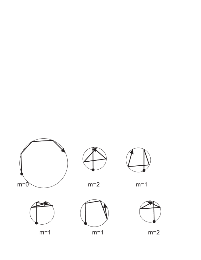
Example 4.

Figure 7 depicts a number of diacyclic configurations for which we obviously have $\delta(R)>0$. The Morse indices are calculated easily. The robot arm in question has four more diacyclic configurations symmetric to the depicted ones. For them, we easily have Morse indices $2,2,2,$ and $0$.

The robot arm in Figure 5 presents more diacyclic configurations with their Morse indices.

5. Concluding remarks

We now wish to outline certain of the natural problems and perspectives suggested by the above results.

1. The most intriguing problem is to find an analog of the generalized Heron polynomial for n-arm, i.e., a univariate polynomial such that its roots give the critical values of area on the moduli space of an arm. Specifically, find out what is the minimal algebraic degree of such a polynomial. Existence of such a polynomial follows from the general results of algebraic geometry using elimination theory but this does not give sufficient information about its algebraic degree.

2. Consider all n-arms with fixed n. What is the exact estimate for the number of diacyclic configurations of such an n-arm? An estimate is provided by the degree of generalized Heron polynomial of the duplicate 2n-gon but this estimate is far not exact and the problem remains unsolved starting with n=4. An exact estimate could be obtained as the algebraic degree of a generalized Heron polynomial sought in the first problem.

3. As we have shown, the oriented area may or may not be a perfect Morse function on the configuration space of n-arm. For which collection of the lengths $l_{i}$ is it perfect, i.e. has the minimal possible number of nondegenerate critical points equal to the sum of Betti numbers of moduli space? In other words, we seek for a criterion of perfectness of oriented area in terms of the lengths of the links. A related problem is to find out if the area can be a function with the minimal possible number of critical points given by the Lusternik-Schnirelmann category of the moduli space. As we have seen, this is the case for equilateral 3-arms. Does the same hold for equilateral 4-arms?

4. An interesting issue is suggested by our description of quasi-cyclic configurations. Namely, as we have seen, each component of quasi-cyclic configurations contains special points of three types: diacyclic, closed cyclic and critical points of the square of the connecting side. Are there any relations between the points of these three types?

5. Analogous problems may be considered for configurations of an arm in three-dimensional space.

References

- [1] Connelly R., Comments on generalized Heron polynomials and Robbins’ conjectures, Discrete Math., 2009, 309, 4192–4196
- [2] Connelly R., Demaine E., Geometry and topology of polygonal linkages, Handbook of discrete and computational geometry, 2nd ed., CRC Press, Boca Raton, 2004, 197–218
- [3] Farber M., Invitation to topological robotics, EMS, Zürich, 2008
- [4] Kapovich M., Millson J., On the moduli space of polygons in the Euclidean plane, J. Differential Geom., 1995, 42(1), 133–164
- [5] Khimshiashvili G., Cyclic polygons as critical points, Proc. I.Vekua Inst. Appl. Math., 2008, 58, 74–83
- [6] Khimshiashvili G., Panina G., Cyclic polygons are critical points of area, Zap. Nauchn. Sem. S.-Peterburg. Otdel. Mat. Inst. Steklov. (POMI), 2008, 360, 8, 238–245
- [7] Khimshiashvili G., Panina G., Siersma D., Zhukova A., Extremal Configurations of Polygonal Linkages, Oberwolfach Preprint, 2011, 24
- [8] Khimshiashvili G., Siersma D., Preprint ICTP, 2009, 047
- [9] Panina G., Zhukova A., Morse index of a cyclic polygon, Cent. Eur. J. Math., 2011, 9(2), 364–377
- [10] Robbins D., Areas of polygons inscribed in a circle, Discrete Comput. Geom., 1994, 12(1), 223–236
- [11] Takens F., The minimal number of critical points of a function on compact manifolds and the Lusternik-Schnirelman cathegory, Invent. Math., 1968, 6, 197–244
- [12] Varfolomeev V., Inscribed polygons and Heron polynomials, Sb.Math., 2003, 194, 3–24 (in Russian)