Higgs Bundles and String Phenomenology
Abstract.
String phenomenology is the branch of string theory concerned with making contact with particle physics. The original models involved compactifying ten-dimensional supersymmetric Yang-Mills theory on an internal Calabi-Yau three-fold. In recent years, this picture has been extended to compactifications of supersymmetric Yang-Mills theory in seven, eight or nine dimensions. We review some of this progress and explain the fundamental role played by Higgs bundles in this story.
Key words and phrases:
Differential geometry, algebraic geometry, string theory, unification1. String Phenomenology
1.1. Particle physics and Grand Unification
To date the most successful description of particle physics is the Standard Model. It is a gauge theory with gauge group and with three fermionic generations of matter:
| (1.1) |
In addition it includes a Higgs field which may soon be discovered at the LHC.
At first sight, these groups and matter representations may look rather random. However it has been known for some time that these representations fit together very nicely if we embed the gauge group into a larger semi-simple group [1]. The simplest choice is
| (1.2) |
In this case, the matter representations are combined into
| (1.3) |
where denotes the two-index ant-symmetric representation of , and denotes the anti-fundamental representation of .
This ‘unification’ of the representations can be continued. The next step is , which unifies the matter representations as well as the neutrino into a single spinor representation of :
| (1.4) |
where the singlet corresponds to the right-handed neutrino. One may continue with , which unifies matter with the Higgs field.
This remarkable bit of group theory could be a simple mathematical curiosity, explained to some extent by anomaly cancellation. However, there is important dynamical evidence that nature makes use of this idea. One of the most compelling pieces of evidence is obtained by adding supersymmetric partners around a TeV, and extrapolating the one-loop running of the gauge couplings upwards. One arrives at the following remarkable picture [2, 3]:
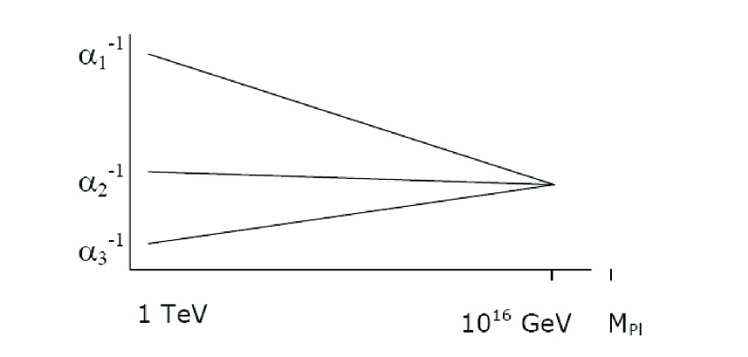
The unification of couplings gives strong evidence for the idea that the three forces of the Standard Model merge into a single force at high energy scales [1]. Such gauge theories go under the name of Grand Unified Gauge Theories or simply GUTs. The convergence of couplings isn’t just an accident of one number coming out right. The fact that the couplings meet just below the Planck scale is also very suggestive. And the picture is fairly robust and in principle independent of supersymmetry; for example it is not materially affected by adding complete multiplets to the theory at intermediate energy scales. Without supersymmetry though, the couplings don’t meet with the same impressive accuracy.
Furthermore, these models not only provide an explanatory framework for some known patterns, but they also yield a new and very characteristic prediction. As was emphasized by Georgi and Glashow, GUT models collect particles with different baryon number in the same multiplet and therefore lead to proton decay, so looking for such decay is one of the best ways to test the hypothesis. In fact, proton decay is one of the few ways we have to directly probe energy scales as large as GeV. It is one of the outstanding questions of particle physics and remains on the experimental agenda. For constraints on Grand Unified models from proton decay, both with and without supersymmetry, see eg. [4, 5, 6].
1.2. The heterotic string
String theory gives a further generalization of this picture by also adding quantum gravity into the mix. We would like to understand how to recover Grand Unification from string theory. This was first achieved by [7] in ’85.
We start with the ten-dimensional heterotic string. Of course its symmetry group is much too big. We want to break this to four-dimensional super-Poincaré invariance and gauge group. To break the Poincaré symmetry, we take the space time of the form
| (1.5) |
It is possible to make a more general Ansatz with a warp factor, but we will not consider it as it is still poorly understood. Preserving super-Poincaré then implies that must be a Calabi-Yau three-fold. To break the gauge symmetry we turn on a non-trivial gauge field along . Four-dimensional supersymmetry then implies that the connection must satisfy the Hermitian Yang-Mills equations:
| (1.6) |
Given a solution to these equations, we may then calculate the effective four-dimensional gauge theory by computing certain Dolbeault cohomology groups. The Standard Model gauge group and the charged matter fields (the ‘visible sector’) all come from Kaluza-Klein reduction of the gauge theory, using just one of the two groups. They are given by the Dolbeault cohomology groups
| (1.7) |
where is the adjoint bundle for one of the gauge groups. The second is said to yield a hidden sector. For this cohomology group counts generators of the gauge group, and for this counts matter fields. So we want to find pairs such that
| (1.8) | |||||
| (1.9) |
We used notation for the quarks and leptons to emphasize that they come in complete multiplets, even though the GUT group is broken. Furthermore, there is a Yoneda product
| (1.10) |
which computes the Yukawa couplings. Here we used the Calabi-Yau condition and the obvious anti-symmetric three-index tensor for to get a number. The Kähler potential (kinetic terms) may not be computed exactly, however there are numerical techniques that allow one to approximate it [8].
Note that even ignoring gravity, string theory has added another level of unification to the story of Grand Unification. In conventional GUTs, matter and gauge fields still appeared as separate entities. But by adding extra dimensions we have managed to unify gauge and matter fields into a single structure: the unique supersymmetric gauge theory with gauge group.
1.3. The landscape
A solution gives only a first (tree level) approximation to the physics. Simple solutions tend to have a large number of moduli, and there are no-go theorems that say that suitable classical solutions without moduli do not exist. The presence of light moduli contradicts known experimental facts, such as the equivalence principle or Big-Bang nucleosynthesis. Furthermore the correct theory of particle physics below a TeV (i.e. the Standard Model) is not supersymmetric. Finding a stable weakly coupled solution is a complicated dynamical problem, and unfortunately many predictions depend on it.
It is by now appreciated that many of the moduli of (in particular complex structure moduli, vector bundle moduli and even some Kähler moduli) can be lifted at tree level, leaving only very few moduli to be stabilized by quantum effects. However the number of such classical solutions which we would like to use as a first approximation to a true solution, keeping fixed, appears to be very large. The existence of an exponentially large number of solutions is well-advertized in the context of -theory flux vacua [9, 10]. It is less well-known that there is an equally large heterotic landscape. This was overlooked for many years, but should have been expected on the basis of heterotic/-theory duality. In particular, the construction of heterotic bundles on elliptic Calabi-Yau manifolds was related in [11] to a Noether-Lefschetz problem, which leads to an exponentially large number of solutions, in the same manner as the -theory landscape.
Let us consider the construction of the MSSM in the heterotic string, on a fixed elliptically fibered Calabi-Yau three-fold . Apart from the Calabi-Yau, the main ingredient is a stable rank five bundle with and . There is a bound on from tadpole cancellation, which will show up as a cut-off below. Using the results of [11] we can make the following rough, Bousso/Polchinski-like estimate for the number of isolated solutions:
| (1.11) |
Here is a cut-off due to tadpole cancellation, which we took conservatively of order . The number to comes from the rank of the homology lattice of a degree five spectral cover over . This version of the landscape arises solely from compactifying the gauge theory, i.e. from the choice of solution to the hermitian-Yang-Mills equation on a rank five bundle, holding everything else (in particular the background ) fixed. As such, it directly affects the parameters in the visible sector.
These numbers are so large that is simply pointless to try to enumerate the set of MSSMs, even on a fixed . However generic solutions are expected to have qualitatively similar particle physics. This lends support to the traditional idea of naturalness in model building: unless there is extra well-motivated structure, dimensionless parameters should be assumed to be of order unity.
1.4. Extension to seven, eight and nine dimensions
In ’85 our picture of string theory was rather limited, and the only known realization of gauge theory was in the context of the heterotic string. However during the duality revolution in the ’90s we learned that lower dimensional gauge theories are also realized in string theory. Thus our excuse for only constructing GUT models from ten-dimensional gauge theory has disappeared. These constructions were carried out in a series of papers in the last three years (some yet to appear).
| dim | stringy realization |
|---|---|
| 10d | heterotic string |
| 9d | strongly coupled type I’ |
| 8d | -theory on ALE |
| 7d | -theory on ALE |
Table 1: Branes with exceptional gauge symmetry in string theory.
The basic summary for the realization of gauge theories in string theory is given in table . There are no supersymmetric gauge theories above ten dimensions, which is why the table ends at the upper end. It is possible to realize gauge theory below 7 dimensions, however then there is not enough room to get chiral matter in 4d. This is why the table ends at the lower end.
The entries for look slightly mysterious: they do not correspond to weakly coupled string theories and the way the non-abelian gauge symmetries arise is not completely obvious, as it involves non-perturbative physics. Obviously we cannot do justice to it here, but let us at least give a very quick summary.
The starting point is -theory, the conjectural non-perturbative completion of eleven-dimensional supergravity. -theory on a smooth space-time does not give rise to non-abelian gauge symmetry, but -theory on a singular ALE space of type ADE gives rise to seven-dimensional super-Yang-Mills theory localized at the singularity, with the corresponding ADE gauge group [12]. An important consistency check is that when we resolve the singularity, quantized -membranes wrapping the vanishing cycles reproduce the off-diagonal components of the Yang-Mills multiplet (i.e. those not proportional to the Cartan generators). -theory on an elliptically fibered space-time with section can be mapped to ten-dimensional type IIb supergravity on the section times a circle. In the limit that the elliptic fiber shrinks to zero, the circle decompactifies. The modular parameter of the elliptic fiber is identified with a varying axio-dilaton of the IIb supergravity, , and the mechanism of non-abelian gauge enhancement is similar to -theory. This is called -theory [13]. -theory on an orbifold gives rise to gauge theory on each of the two walls. This is the Horava-Witten picture [14]. By shrinking the interval, we recover the weakly coupled heterotic string. By instead compactifying on and shrinking it, we get the type I’ theory [15]. In each of these contexts, when the non-abelian gauge symmetry is of type , or , we can often extrapolate to a weakly coupled -brane configuration in perturbative string theory, but for the exceptional cases this is not possible. These issues were only understood after the non-perturbative behaviour of string theory became clearer in the ’90s.
In this review we will be firmly focused on the Yang-Mills theory itself, without much consideration of its origins. Part of the reason for this is that if we want to consider exceptional gauge groups in higher dimensions, then the string point of view involves singular geometries and strongly coupled physics, whereas the higher dimensional Yang-Mills theory is weakly coupled in the derivative expansion. We will briefly explain how to connect with string theory in section 2.4. The upshot will be that we can reconstruct the local geometry from the Yang-Mills theory. The type I’ story requires a separate discussion, which will not be attempted here.
Unification with eight-dimensional Yang-Mills theory was initiated in [16, 17, 18] and is currently the most developed and best understood of the new cases. The main reason for this is that in even dimensions one can use the powerful techniques of complex and algebraic geometry. The seven-dimensional story was initiated in [19] and the nine-dimensional story will appear in [20].
The strategy that we will use is similar to the heterotic string. The main new idea is that instead of Hermitian-Yang-Mills bundles, we have to consider their close cousins: Higgs bundles. This consists of a bundle together with a map
| (1.12) |
where is a suitable twisting bundle. The connection on and the ‘Higgs field’ have to satisfy certain versions of Hitchin’s equations, which we discuss below. (The terminology is standard and the field has no direct relation to the Higgs boson of the Standard Model).
2. Higgs bundles
2.1. Dimensional reduction
The maximally supersymmetric Yang-Mills theory in dimensions is uniquely determined by the choice of gauge group. Its Lagrangian can be obtained by dimensional reduction from the supersymmetric Yang-Mills theory. Therefore we would expect that the BPS conditions can be obtained from dimensional reduction of the hermitian Yang-Mills equations (1.6).
There is a well-known analogous story involving reduction of the hermitian Yang-Mills equations, aka the ASD equations. Reducing to three dimensions yields the Bogomolnyi equations:
| (2.1) |
The reduction to two dimensions is known as Hitchin’s equations:
| (2.2) |
where denotes contraction with the Kähler form. These equations turn out to have many applications, and several variants have been considered. We will be interested in some of its higher dimensional variants.
Indeed let us now consider the dimensional reduction of the hermitian Yang-Mills equations (1.6), relevant for compactifications of Yang-Mills down to four dimensions. For Yang-Mills on we get , as well as equations (2.2) above on . For Yang-Mills on we get
| (2.3) |
This is the real version of Hitchin’s equations, defined on a real three-manifold . The gauge and Higgs field can be assembled into a complex gauge field , and the first two equations above assert that this is a complex flat connection on . For Yang-Mills we compactify on , where is a five-manifold given by an -fibration over a Kähler surface. Denote complex coordinates on the base by and along the by . Then we get
| (2.4) |
where denotes the components orthogonal to the . This is a higher dimensional generalization of the Bogomolnyi equations.
2.2. Compactification of eight-dimensional SYM
We can now summarize the main results of the Kaluza-Klein reduction of the higher dimensional Yang-Mills theory to four dimensions. We take the supersymmetric Yang-Mills theory as our main example [16, 17, 11, 21]. The Higgs bundle will be defined on a compact Kähler surface . As we have seen, the bosonic fields are given by a connection on a bundle on , and a complex Higgs field valued in . The twisting by the canonical bundle is required to preserve the super-Poincaré invariance. The equations are given by
| (2.5) |
In practice, we actually need meromorphic Higgs bundles, or in recent physics language, we need to insert certain surface operators along a curve in . The simplest such defects lead to parabolic Higgs bundles [22]. They may be thought of as arising from integrating out hypermultiplets living on , which become dynamical when we embed the gauge theory into a compact model. We will not discuss these defects explicitly here.
Given a solution to these equations, we would like to know the effective gauge theory in four dimensions obtained from the Kaluza-Klein reduction of the eight-dimensional gauge theory on . We define a two-term complex :
| (2.6) |
The gauge theory is derived by computing the hypercohomology groups
| (2.7) |
For this counts generators of the gauge group, and for it counts matter fields. We can compute the Yukawa couplings from a Yoneda product
| (2.8) |
and conjecturally we can even numerically approximate the hermitian-Einstein metric and therefore the kinetic terms [22]. Of course this parallels the analogous statements for the heterotic string we discussed earlier.
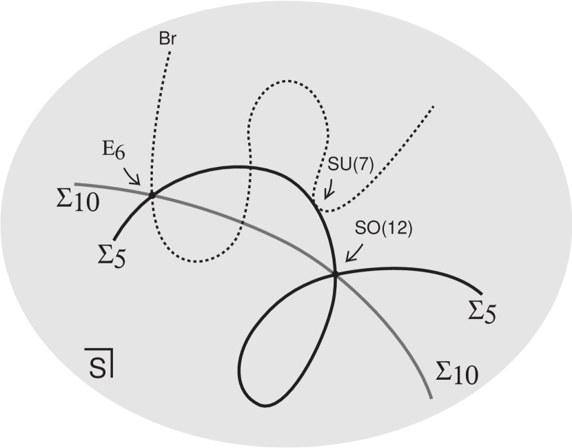
These statements perhaps seem somewhat abstract. It is often possible to give more intuitive pictures for the wave functions of the massless modes. The main picture in this regard is that a generic zero of can be interpreted as a vortex string on , and as is well known one tends to get charged zero modes localized on such a vortex. Thus while the wave functions of the four-dimensional gauge fields are spread out over , the wave functions of charged matter such as the or of an GUT tends to be localized on some Riemann surface in , see figure 2. For super-Yang-Mills theory compactified on we get a similar picture, with gauge fields spread over but chiral matter in the or generically localized at points on . Such localization leads to interesting possibilities for phenomenology. But for non-generic configurations the intuition can be misleading, and the advantage of the above formulation is that it is precise and general.
2.3. Higgs/spectral correspondence
Now that we have the general statements, we need a good method for constructing solutions and computing the hypercohomology groups. Hitchin’s equations are highly non-linear, so trying to solve them in closed form is bound to fail. Instead we will make use of two standard techniques. The first is the technique of splitting up the equations in ‘-terms’ and ‘-terms’, i.e.:
-
•
a pair of complex equations:
-
•
a moment map:
The strategy is then to temporarily ignore the -terms, and focus on the -terms, which we can solve exactly up to complexified gauge transformations. This amounts to focussing on the holomorphic structure and ignoring the hermitian metric. Once we have done that, we can go back and try to apply some powerful results in geometric invariant theory regarding -flatness.
To solve the -term equations, we use the second essential tool, namely the Higgs/spectral correspondence. Essentially it turns the problem of constructing solutions to the -terms into an ‘abelianized’ version which is much simpler to solve. To avoid the somewhat intricate group theory of , we will take to be a rank vector bundle transforming in the fundamental representation of .
The Higgs/spectral correspondence states that there is an equivalence
| (2.9) |
mapping the (holomorphic data of the) Higgs bundle to its spectral data. That is, we interpret as a map , and then we fiberwise replace by the eigenvalues and by the eigenvectors. The relation can concisely expressed through a short exact sequence
| (2.10) |
where , is pull-back to the total space of the canonical bundle, and is the tautological section of . For future use, we also denote the total space of by . The similarity to our notation for the heterotic Calabi-Yau three-fold is not entirely coincidental. There are versions of this correspondence also for meromorphic Higgs bundles.
Such spectral sheaves are fairly simple to write down explicitly, certainly compared to solving non-abelian equations. As an example relevant for phenomenological models, let us consider breaking an gauge group to . This requires writing down an Higgs bundle over , where the structure group is the commutant of in the (complexified) . By the Higgs/spectral correspondence, the data of such an Higgs bundle is given by
-
•
the spectral cover in (the support of ), given explicitly by a degree five polynomial;
-
•
the spectral line bundle in , which may be specified by writing an explicit divisor on and putting . We then define , where is the inclusion and is the push-forward.
Here we can see the Noether-Lefschetz problem rearing its head. We need to choose a curve in a surface in a three-fold. Simple examples constructed by hand will have many moduli. But if the curve is sufficiently ‘generic’ then deforming the surface or the three-fold will destroy the curve, in other words the corresponding deformation moduli are stabilized. However finding the most rigid solutions requires us to solve a complicated Noether-Lefschetz problem, and the number of solutions grows exponentially with the rank of . This brings us back to the landscape problem. If these vacua are really stable after including quantum corrections (and most are probably not), then we’d have to ask who lives in the other mathematically consistent universes, and how was our universe able to solve the complicated computational problem of finding the most rigid, stable solutions. It is probably best to focus on general features of the whole class of solutions, rather than on individual solutions.
Leaving such questions aside, another important point about the separation into -terms and -terms is that changing the hermitian metric on does not affect the hypercohomology groups . Therefore the low energy spectrum and Yukawa couplings are independent of the hermitian metric on , and in fact they may be computed directly in terms of the spectral sheaf using Ext groups. Needless to say, this simplifies one’s life tremendously.
This takes care of the -terms. The -terms (i.e. the moment map equation) may now be interpreted as an equation for the hermitian metric on , and a solution (if it exists) is called a hermitian-Einstein metric. As mentioned already, solving this equation in closed form is virtually impossible. Instead one would like to appeal to a Higgs bundle version of the Donaldson-Uhlenbeck-Yau theorem:
A unique HE metric exists the Higgs bundle is poly-stable.
A Higgs bundle is stable if for every Higgs sub-bundle , we have
| (2.11) |
The slope is defined to be the ratio of the degree of (with respect to some choice of Kähler form) and the rank of . A Higgs bundle is said to be poly-stable if it is the sum of stable Higgs bundles with the same slope.
The beauty of this type of statement is that existence of the hermitian-Einstein metric is a differential-geometric criterion, whereas poly-stability is an algebro-geometric criterion. In particular, one can easily translate the requirement of stability for the Higgs bundle to stability for the spectral sheaf . Unfortunately the proven versions of this correspondence do not suffice in our context, because we really need certain meromorphic incarnations of Higgs bundles. In particular, the stability condition depends on boundary data associated to the defect/surface operator, as is well-known for parabolic Higgs bundles. Modulo that issue however, we see that the Higgs/spectral correspondence answers the problem posed at the beginning of this section: constructing solutions and understanding the effective theory boils down almost entirely to constructing and studying suitable spectral sheaves .
In other dimensions, the story is in principle similar, but less understood. In -theory we were dealing with (2.3), which describes complex flat connections on a real manifold . Up to complexified gauge transformations, we can exchange such a complex flat connection for spectral data. In this case, the spectral cover corresponds to a Lagrangian -brane in the cotangent bundle [19], and the spectrum is computed by Floer cohomology groups of the -brane.
2.4. Spectral/ALE correspondence
Although we have claimed that our constructions are realized in string theory, the reader may be puzzled that the descriptions we have obtained seem to look very different from the traditional descriptions of -theory, -theory and type I’, which we briefly touched on in section 1.4. Four-dimensional compactifications of -theory are usually said to involve elliptically fibered Calabi-Yau manifolds with a configuration for a certain three-form (mathematically, a 2-gerbe with some additional properties). Four-dimensional compactifications of -theory are usually said to involve manifolds with -holonomy and a flat three-form (mathematically, a flat 2-gerbe). So far these did not yet appear in our story. In order to see the relation, we need another dictionary: the spectral/ALE correspondence [23, 11, 19].
In order to avoid the somewhat complicated representation theory of , we will illustrate the correspondence by focussing on Higgs bundles and -type ALE fibrations. Consider the ALE fibration given by
| (2.12) |
The are sections of certain line bundles on . Let us define a fibration whose fibers over a point on are the lines defined by
| (2.13) |
The second equation specifies points in the -plane, hence defines an -fold covering , which we identify with the spectral cover. We also get a natural projection by replacing each line with a point. We further have a natural inclusion . Then the spectral/ALE correspondence is given by the ‘cylinder’ maps and :
| (2.14) |
where denotes a certain primitive part of the cohomology, and and denote certain compactifications. In particular this maps the class of the spectral line bundle in to the Deligne cohomology class of a -gerbe on . The more sophisticated version for exceptional gauge groups was described in [23, 11]. Essentially this mapping establishes a isomorphism of certain Hodge structures associated to the spectral cover and ALE sides.
The spectral/ALE correspondence exists for any gauge group, but the group theory tends to get more involved when we go away from the unitary groups. It so happens that for model building, which is the most relevant case phenomenologically, the group theoretic aspects simplify somewhat. A configuration in an gauge theory with an unbroken group corresponds to the following ALE fibration over [11]:
| (2.15) |
Here the are sections of certain line bundles over . Note that we can easily put this in the form of a Weierstrass model by making some coordinate redefinitions. Under the spectral/ALE correspondence this gets mapped to an spectral cover which decomposes into various pieces. One of these pieces is a five-fold cover of , given by a degree five equation in the total space of :
| (2.16) |
Here is a local coordinate on the fiber of . This is precisely the spectral cover for the fundamental representation of the Higgs bundle mentioned in section 2.3. The intersection of with the zero section yields a curve where the singularity of the generic ALE fiber (2.15) further degenerates to type , as one can easily check. This is the curve where matter fields on the and of propagate, see figure 2. One also gets a ten-fold covering , the spectral cover in the anti-symmetric representation of our Higgs bundle in section 2.3. Its intersection with the zero section yields a curve where the singularity of the ALE fiber degenerates to . This is the curve where the and matter of propagate, again see figure 2. One gets various further degenerations in higher codimension. For details of this construction, see [11].
Using the spectral/ALE correspondence for we obtain an elliptic Calabi-Yau four-fold with boundary together with a Deligne cohomology class. We can then proceed to glue into a compact Calabi-Yau four-fold [11]. In this way we recover the traditional description of -theory vacua.
In the -theory context, the spectral data was given by a Lagrangian -brane in . Under the spectral/ALE correspondence, it gets mapped to an ALE fibration over with a flat 2-gerbe, and with singularities at the location of non-abelian gauge groups and charged chiral matter. We have argued that this seven-dimensional non-compact manifold should admit a metric with holonomy [19]. This should then be glued into a compact manifold.
Note that in the traditional descriptions, we are dealing with singular spaces. For example to get an gauge theory in four dimensions from -theory, we needed type quotient singularities along a section isomorphic with which further degenerate in higher codimension. Of course, the problem with singularities is that they are singular. In order to do physics, we need some way to ‘smooth’ these singularities. The traditional way to do this is by making a crepant resolution (in physics terms, using /-duality and moving out on the Coulomb branch). Then one can quantize solitons wrapped on the exceptional cycles to deduce some of the physics. Unfortunately this extrapolation is not valid at the level of -terms and it obscures many aspects of the physics which are relevant for phenomenology. For example a proper definition of the -theory 2-gerbe and the analogue of its hypercohomology groups has not yet been given, in part because the 2-gerbe may obstruct such resolutions. Furthermore it is not clear how to extend this approach to other setting like -theory on manifolds with singularities, where no natural resolution is available. The Higgs bundle/Yang-Mills theory approach yields another way to smooth the singularities, which has proven more useful for the questions discussed here.
2.5. Some open problems
Here we collect some open mathematical problems. They were mostly already pointed out in the text, but we group them here for convenience. It is not meant to be a complete list, and we only list questions that fit in the scope of this review.
-
•
Explicit constructions. It is an open problem to find non-abelian solutions to the -term part of the Yang-Mills-Higgs equations in odd dimensions, given in equations (2.3) and (2.4). Furthermore, given a solution, one would like an effective method for computing hypercohomology groups. For solving (2.3) one could appeal to Donaldson-Corlette. However as we mentioned, for phenomenological applications one should add source terms to (2.3) and (2.4) along a submanifold. An interesting sub-problem is to classify the most general supersymmetric boundary conditions (source terms).
A class of non-abelian solutions for the type I’ case will appear in [20]. The strategy there is to assume an symmetry and make use of the Fourier-Mukai transform to turn the question into a holomorphic problem. For the -theory models we could use a similar strategy, by using mirror symmetry for . Presumably there are other approaches. Is it possible to give a more general construction?
The equations encountered in this review often reappear in other contexts, see eg. [24] or the literature on knot invariants. The source terms are said to be associated to ‘defect operators.’ Thus a positive answer could also be helpful in other contexts.
-
•
D-flatness. Once we can construct solutions to the -term equations, we still have to solve the moment map equation. This is called proving -flatness in physics terminology. The standard strategy is to formulate some type of stability condition, and then to try and prove an analogue of the Donaldson-Uhlenbeck-Yau theorem for Hermitian-Yang-Mills connections.
In the holomorphic case one can make natural conjectures for the stability criterion (including source terms), but a proof of -flatness is missing. Mochizuki has given proofs for certain classes of parabolic Higgs bundles, which unfortunately are slightly different from the Higgs bundles considered here. For the odd dimensional cases, it is not clear to us what the correct stability condition should be.
-
•
Deformation theory. To find the low energy effective action, we needed to understand the infinitesimal deformations of the Higgs bundle. They were classified by certain hypercohomology groups of the Higgs bundle. In the spectral cover picture, one is asking for the infinitesimal deformations of a coherent sheaf or a Lagrangian brane with flat connection. These are classified by Ext groups or Floer cohomology groups respectively.
But we also had a third picture: ALE fibrations with a 2-gerbe, satisfying some additional conditions. (The conditions in -theory are somewhat complicated to state; see appendix C of [16] where a compactified version of ALE fibrations is considered). So we have a natural question: what classifies the first order infinitesimal deformations in the ALE fibration picture? And what are the analogues of the Yoneda pairing and the higher Massey-like products, which compute Yukawa couplings and higher order interactions?
It is not clear to us how to answer this question, and maybe a good answer is not possible. There are many well-understood spectral cover configurations that get mapped to poorly understood ALE-fibrations. As a simple example, one may consider a non-abelian bundle on a degenerate non-reduced cover. This should get mapped to an ALE fibration with singularities, and some kind of non-abelian 2-gerbe along the singularities, whatever that means exactly. Such configurations cannot be lifted to the resolution, but should be included in the general formulation. More complicated examples can be found in [22]. Thus understanding the -gerbe is an important part of the problem. One could further ask about stability conditions in this picture. This is also poorly understood.
-
•
Local versus global. ALE fibrations are said to be local because they are non-compact. For string phenomenology, we think of them as a local piece of a compact manifold, and eventually we would like to embed them in a concrete global model, i.e. in a compact manifold. In the context of -theory there has been a lot of progress on this question. Questions remain, but this is outside the scope of this review. In the context of -theory, we would like to embed our ALE fibration in a compact holonomy manifold. The problem here is obvious: there are very few constructions of compact manifolds and none appears to be suitable for compactifying our ALE fibrations.
-
•
Finite or infinite landscape. We discussed some crude estimates for the number of solutions of the hermitian-Yang-Mills or Hitchin equations which reproduce the supersymmetric standard model or a unified extension thereof. In toy models of flux vacua it appears that the true number of solutions can be much larger. In fact, there is a basic question if the true number of solutions is even finite. The prevailing opinion is that it should be finite, but we recently constructed an infinite sequence which appears to be stable and evades the known no-go theorems [25]. (It should be remembered that proving stability is of course the hardest part). Such infinite sequences would address some concerns raised in [26].
There are of course also many interesting physical questions. In particular one would like to get an interesting physical prediction that distinguishes the extra-dimensional models from conventional four-dimensional models. Once we have done the Kaluza-Klein reduction, we are working within four-dimensional effective field theory. So are there processes where we might see the extra dimensions in the foreseeable future? The answer appears to be yes, at least in principle. Proton decay probes the GUT scale and could provide such characteristic signatures [27, 28, 29]. The extra dimensions become important at the GUT scale and the proton feels the higher dimensional interactions. For further questions and developments, see the talk by S. Schäfer-Nameki at this conference [30], and the additional reviews [31, 32, 33, 34, 35].
Acknowledgements: I would like to thank the organisers of String-Math 2011 for an inspiring conference. I would also like to thank R. Donagi and T. Pantev for collaboration on the material presented here, and R. Donagi and the referee for comments on the manuscript.
References
- [1] H. Georgi and S. L. Glashow, “Unity Of All Elementary Particle Forces,” Phys. Rev. Lett. 32, 438 (1974).
- [2] H. Georgi, H. R. Quinn and S. Weinberg, “Hierarchy Of Interactions In Unified Gauge Theories,” Phys. Rev. Lett. 33, 451 (1974).
- [3] S. Dimopoulos, S. Raby and F. Wilczek, “Supersymmetry And The Scale Of Unification,” Phys. Rev. D 24, 1681 (1981).
- [4] S. Raby, “Proton decay,” hep-ph/0211024.
- [5] P. Nath and P. Fileviez Perez, “Proton stability in grand unified theories, in strings and in branes,” Phys. Rept. 441, 191 (2007) [arXiv:hep-ph/0601023].
- [6] G. Senjanovic, “Proton decay and grand unification,” AIP Conf. Proc. 1200, 131 (2010) [arXiv:0912.5375 [hep-ph]].
- [7] P. Candelas, G. T. Horowitz, A. Strominger and E. Witten, “Vacuum Configurations for Superstrings,” Nucl. Phys. B 258, 46 (1985).
- [8] M. R. Douglas, R. L. Karp, S. Lukic and R. Reinbacher, “Numerical solution to the hermitian Yang-Mills equation on the Fermat quintic,” JHEP 0712, 083 (2007) [arXiv:hep-th/0606261].
- [9] R. Bousso and J. Polchinski, “Quantization of four form fluxes and dynamical neutralization of the cosmological constant,” JHEP 0006, 006 (2000) [arXiv:hep-th/0004134].
- [10] F. Denef and M. R. Douglas, “Distributions of flux vacua,” JHEP 0405, 072 (2004) [arXiv:hep-th/0404116].
- [11] R. Donagi and M. Wijnholt, “Higgs Bundles and UV Completion in F-Theory,” arXiv:0904.1218 [hep-th].
- [12] E. Witten, “String theory dynamics in various dimensions,” Nucl. Phys. B 443, 85 (1995) [arXiv:hep-th/9503124].
- [13] C. Vafa, “Evidence for F-Theory,” Nucl. Phys. B 469, 403 (1996) [arXiv:hep-th/9602022].
- [14] P. Horava and E. Witten, “Heterotic and type I string dynamics from eleven dimensions,” Nucl. Phys. B 460, 506 (1996) [arXiv:hep-th/9510209].
- [15] J. Polchinski and E. Witten, “Evidence for Heterotic - Type I String Duality,” Nucl. Phys. B 460, 525 (1996) [arXiv:hep-th/9510169].
- [16] R. Donagi and M. Wijnholt, “Model Building with F-Theory,” arXiv:0802.2969 [hep-th], to appear in ATMP.
- [17] C. Beasley, J. J. Heckman and C. Vafa, “GUTs and Exceptional Branes in F-theory - I,” JHEP 0901, 058 (2009) [arXiv:0802.3391 [hep-th]].
- [18] H. Hayashi, R. Tatar, Y. Toda, T. Watari and M. Yamazaki, “New Aspects of Heterotic–F Theory Duality,” Nucl. Phys. B 806, 224 (2009) [arXiv:0805.1057 [hep-th]].
- [19] T. Pantev and M. Wijnholt, “Hitchin’s Equations and M-Theory Phenomenology,” J. Geom. Phys. 61, 1223 (2011) [arXiv:0905.1968 [hep-th]].
-
[20]
T. Pantev and M. Wijnholt,
“Unification and type I’.”
For an overview, see http://www.math.unm.edu/ vassilev/goldensands/tpantev.pdf. - [21] H. Hayashi, T. Kawano, R. Tatar and T. Watari, “Codimension-3 Singularities and Yukawa Couplings in F-theory,” Nucl. Phys. B 823, 47 (2009) [arXiv:0901.4941 [hep-th]].
- [22] R. Donagi and M. Wijnholt, “Gluing Branes, I,” arXiv:1104.2610 [hep-th].
- [23] G. Curio and R. Y. Donagi, “Moduli in N = 1 heterotic/F-theory duality,” Nucl. Phys. B 518, 603 (1998) [arXiv:hep-th/9801057].
- [24] A. Kapustin and E. Witten, “Electric-magnetic duality and the geometric Langlands program,” arXiv:hep-th/0604151.
- [25] R. Donagi, M. Wijnholt.
- [26] M. Dine and N. Seiberg, “Is The Superstring Weakly Coupled?,” Phys. Lett. B 162, 299 (1985).
- [27] T. Friedmann and E. Witten, “Unification scale, proton decay, and manifolds of G(2) holonomy,” Adv. Theor. Math. Phys. 7, 577 (2003) [arXiv:hep-th/0211269].
- [28] I. R. Klebanov and E. Witten, “Proton decay in intersecting D-brane models,” Nucl. Phys. B 664, 3 (2003) [arXiv:hep-th/0304079].
- [29] R. Donagi and M. Wijnholt, “Breaking GUT Groups in F-Theory,” arXiv:0808.2223 [hep-th], to appear in ATMP.
- [30] S. Schäfer-Nameki, “F-theory: global aspects and phenomenology,” talk at this conference.
- [31] J. J. Heckman and C. Vafa, “From F-theory GUTs to the LHC,” arXiv:0809.3452 [hep-ph].
- [32] M. Wijnholt, “F-Theory, GUTs and Chiral Matter,” arXiv:0809.3878 [hep-th].
- [33] J. J. Heckman, “Particle Physics Implications of F-theory,” Submitted to: Ann.Rev.Nucl.Part.Sci. [arXiv:1001.0577 [hep-th]].
- [34] M. Wijnholt, “F-theory and unification,” Fortsch. Phys. 58, 846 (2010).
- [35] T. Weigand, “Lectures on F-theory compactifications and model building,” Class. Quant. Grav. 27, 214004 (2010) [arXiv:1009.3497 [hep-th]].